Fast gradient-free optimization of excitations in variational quantum eigensolvers

Abstract

We introduce ExcitationSolve, a fast globally-informed gradient-free optimizer for physically-motivated ansätze constructed of excitation operators, a common choice in variational quantum eigensolvers. ExcitationSolve is to be classified as an extension of quantum-aware and hyperparameter-free optimizers such as Rotosolve, from parameterized unitaries with generators $G$ of the form $G^{2}=I$, e.g., rotations, to the more general class of $G^{3}=G$ exhibited by the physically-inspired excitation operators such as in the unitary coupled cluster approach. ExcitationSolve is capable of finding the global optimum along each variational parameter using the same quantum resources that gradient-based optimizers require for a single update step. We provide optimization strategies for both fixed- and adaptive variational ansätze, as well as a multi-parameter generalization for the simultaneous selection and optimization of multiple excitation operators. Finally, we demonstrate the utility of ExcitationSolve by conducting electronic ground state energy calculations of molecular systems and thereby outperforming state-of-the-art optimizers commonly employed in variational quantum algorithms. Across all tested molecules in their equilibrium geometry, ExcitationSolve remarkably reaches chemical accuracy in a single sweep over the parameters of a fixed ansatz. This sweep requires only the quantum circuit executions of one gradient descent step. In addition, ExcitationSolve achieves adaptive ansätze consisting of fewer operators than in the gradient-based adaptive approach, hence decreasing the circuit execution time.

1 Introduction

The choice of ansatz for the parameterized or variational quantum circuit plays a crucial role in the variational quantum eigensolver (VQE) [1], which aims to prepare the ground state of a Hamiltonian and find the corresponding ground state energy. The Hamiltonian can describe, e.g., an electronic structure problem in a molecule or material [1, 2, 3, 4]. Physically-motivated ansätze, such as a composition of excitation operators like single and double fermionic excitations in the Unitary Coupled Cluster (UCCSD) ansatz [1], are particularly relevant because of their guarantees of producing physically plausible states. By design, relevant physical properties of an initial reference state, typically the Hartree-Fock (HF) state, are conserved, such as the number of electrons or spin symmetries. Furthermore, number-conserving, yet hardware-efficient approaches, such as qubit-excitation based (QEB) ansätze [5] exist, most prominently appearing in the Qubit Coupled Cluster Singles Doubles (QCCSD) ansatz [6]. In contrast, problem-agnostic ansätze like generic hardware-efficient ansätze might yield physically implausible states and energies by, e.g., not conserving the number of particles [7]. These ansätze are composed of parameterized qubit rotations. The implications of ansatz choice are visualized in Fig. 1.

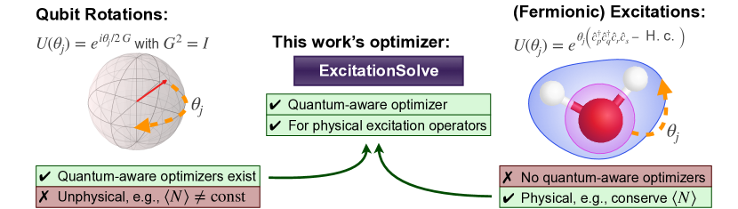
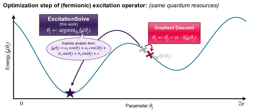
Figure 1: Schematic overview of our work. Top: while hardware-efficient ansätze, typically composed of parameterized rotations, allow for fast quantum-aware optimization [8, 9, 10, 11], they do not preserve physical properties [7], e.g., vary the average particle number $\langle N\rangle$, the opposite is true for physically-motivated ansätze such as those assembled from fermionic excitation operators [1]. Our new optimizer, ExcitationSolve, fills this gap and combines fast optimization with physical guarantees. Bottom: ExcitationSolve (purple) relies on the same quantum resources, i.e., same number of energy measurements, to jump to the global energy minimum along a single parameter $\theta_{j}$, as a gradient-based optimizer (red) evaluating and following the (partial) derivative in $\theta_{j}$. The latter does not consider global information of the energy landscape, thus being limited to a local parameter region. Note that since gradient descent is based on the full gradient evaluated over $N$ parameters, ExcitationSolve in fact performs $N$ update steps while gradient descent updates locally once.

 

After specifying the variational ansatz $U(\bm{\theta})$, its $N$ parameters $\bm{\theta}\in[-\pi,\pi]^{N}$ have to be optimized to prepare the desired ground state. This optimization happens iteratively in a hybrid loop involving a quantum computer to evaluate the energy and a classical computer to optimize the parameters. On the quantum computer we evaluate the expectation value $\braket{\psi(\bm{\theta})}{H}{\psi(\bm{\theta})}$ of the Hamiltonian $H$ with respect to prepared $n$-qubit state $\ket{\psi(\bm{\theta})}=U(\bm{\theta})\ket{\psi_{0}}$, as a function of the current parameters. The energy landscape $f(\bm{\theta})$ we want to minimize can be written as

$$f(\bm{\theta})=\braket{H}=\braket{\psi_{0}}{U^{\dagger}(\bm{\theta})HU(\bm{\theta})}{\psi_{0}}.$$ (1)

Note that an adaptive ansatz can be also employed, where operators/gates are iteratively added to the ansatz during the optimization. This concept was first introduced as ADAPT-VQE [12]. However, the VQE optimization problem is generally challenging because the energy landscape is a $N$-dimensional trigonometric function [11], leading to a large number of local minima, many of which are sub optimal [13, 14, 15, 16]. Therefore, gradient-based optimizers (e.g., gradient descent, Adam [17] or BFGS [18, 19, 20, 21]) as well as a gradient-free black-box optimizers (e.g., COBYLA [22], SPSA [23, 24]) struggle to navigate the complex energy landscape as for larger molecules or materials.

So-called quantum-aware optimizers pose a promising alternative since they leverage problem-specific knowledge to navigate the energy landscape more efficiently. A prominent example is the Rotosolve optimization method [8], which was simultaneously proposed under the term Sequential Minimal Optimization (SMO) [9], as well as analogously mentioned in Refs. [10, 11]. Rotosolve globally optimizes parameterized operators based on the closed form of the energy landscape, thus leveraging the operator-specific properties to significantly reduce the required quantum resources [8]. This provides an efficient alternative to gradient-based optimization. However, the type of parameterized operators or gates incorporated in the ansatz must be compatible with the quantum-aware optimizer. The applicability of Rotosolve is limited to unitaries with self-inverse generators, e.g., (Pauli) rotation gates, although generalizations were suggested [25]. While the more complicated unitaries relevant for quantum chemistry applications can be decomposed into fixed entangling gates and parameterized rotations [26], Rotosolve’s performance degrades as it then overestimates the required number of energy evaluations.

In this work, we combine the advantages of incorporating excitation operators in physically-motivated VQE ansätze with the effectiveness of quantum-aware optimizers. We introduce ExcitationSolve, a fast globally-informed gradient-free optimizer for ansätze composed of excitation operators. ExcitationSolve is quantum-aware since we know the analytical form of the energy landscape in one parameter (or a subset of parameters) for excitation operators, which is a (multi-dimensional) second-order Fourier series. This applies to fermionic excitations [1], qubit excitations [5, 6], and Givens rotations [27] – not limited to single and double excitations. ExcitationSolve can be applied to fixed and adaptive VQE ansätze as in the UCCSD ansatz [1] and ADAPT-VQE [12], respectively. A schematic summary of our work is provided in Fig. 1.

In Sec. 2 we introduce the framework of the ExcitationSolve algorithm, followed by a description of operator classes covered by the algorithm in Sec. 2.1. In Sec. 2.2 we describe how ExcitationSolve can be utilized to globalize the selection criterion in ADAPT-VQE. Section 2.3 considers the multi-dimensional generalization of ExcitationSolve, showcasing how higher-dimensional reconstructions can be used to enhance the optimization of multiple variational parameters in both fixed VQE and ADAPT-VQE. We further generalize ExcitationSolve to multiple occurrences of the same variational parameter in Sec. 2.4, making it compatible with ansätze constituted of higher-order product formulas or multiple Trotter steps. To complete the scope of applicability of ExcitationSolve, Sec. 2.5 covers the most generic case of a multi-parameter optimization where each parameter may occur multiple times. Section 3 provides simulated experiments comparing ExcitationSolve to optimizers commonly used in VQE literature for fixed- and adaptive ansätze exemplified by ground state preparation of small molecules. Here, Sec. 3.1 focuses on the setting of a fixed ansatz scenario, while Sec. 3.2 targets adaptive ansätze. In Sec. 3.3 we explore the utility of ExcitationSolve in the realm of strongly correlated systems and further employ 2D optimization to accelerate convergence. Last, Sec. 3.4 demonstrates how the different optimizers perform under the influence of shot noise. Section 4 concludes our work with a discussion. Details on the used methodology can be found in Sec. 5 and Appendix C, while Appendix B provides mathematical derivations and proofs.

2 ExcitationSolve algorithm

In this section, we introduce the quantum-aware optimization algorithm ExcitationSolve, which readily extends Rotosolve-type optimizers [8, 9] to excitation operators, which obey the following more general form. Throughout this work, we assume variational ansätze $U(\bm{\theta})$ consisting of a product of unitary operators $U(\theta_{j})$ of the generic form

$$U(\theta_{j})=\exp(-i\theta_{j}G_{j}),$$ (2)

depending on a single parameter $\theta_{j}$ each (the $j$-th component of $\bm{\theta}$). Most importantly, with the Hermitian generators $G_{j}$ fulfilling $G_{j}^{3}=G_{j}$. Note that any generator with $G_{j}^{2}=I$ (the prerequisite of Rotosolve) fits into this description. However, this work is concerned with the class of excitation operators because their generators fulfill $G_{j}^{3}=G_{j}$ and, importantly, $G_{j}^{2}\neq I$.

In the following, we first present the analytic form of the energy landscape when varying a single parameter in an operator of the aforementioned structure, and, second, how this is exploited to derive an optimization algorithm. The analytic form of the energy with respect to a single parameter $\theta_{j}$ associated with some generator $G_{j}$ is a finite Fourier series (also known as a trigonometric polynomial) of second-order with period $2\pi$ and has the form

$$f_{\bm{\theta}}(\theta_{j})=a_{1}\cos(\theta_{j})+a_{2}\cos(2\theta_{j})+b_{1}\sin(\theta_{j})+b_{2}\sin(2\theta_{j})+c.$$ (3)

Here, the notation $f_{\bm{\theta}}(\theta_{j})$ refers to the energy landscape $f(\bm{\theta})$ from Eq. (1) with all parameters being fixed except $\theta_{j}$. The five coefficients $a_{1},a_{2},b_{1},b_{2},c$ are independent of the parameter $\theta_{j}$ but may depend on the remaining parameters $\theta_{i\neq j}$, which is detailed in the constructive proof in Appendix B.1. In order to determine these five coefficients, we need energy values in at least five distinct configurations of the parameter $\theta_{j}$. For five evaluations, the coefficients are the solution to the linear equation system, whereas for more than five evaluations, the overdetermined equation system can be solved using either the least square method or truncated (fast) Fourier transform. Section 5.2 discusses how this relates to noise robustness.

The proposed optimization algorithm ExcitationSolve (cf. Algorithm 2) iteratively sweeps through the parameters $\bm{\theta}$, reconstructs the energy landscape per parameter $\theta_{j}$ analytically, globally minimizes the reconstructed function classically, and assigns the parameter $\theta_{j}$ to the value where the global minimum is attained. The order in which the parameters $\theta_{j}$ are optimized can be chosen freely. This process is repeated until convergence, which is defined by a threshold criterion on the absolute or relative energy reduction of the last parameter sweep. In this algorithm, the quantum computer is used exclusively to obtain energy evaluations while the reconstruction and subsequent minimization of the energy landscape is performed on a classical computer. To determine the minimum energy and corresponding parameter classically, we utilize a companion-matrix method [28], which is a direct numerical method detailed in Sec. 5.1. Importantly, in each optimization step, the previously determined minimum energy can be reused, requiring only an additional four parameter shifts to reconstruct the energy landscape along the next parameter. Footnote 2 describes the exact algorithmic details.

Hardware Resources: Quantum Computer (QC), Classical Computer (CC)

Input: Initial parameters $\bm{\theta}^{(0)}=\bm{0}$, HF/init. energy $E^{(0)}=f(\bm{\theta}^{(0)})$, HF/init. state $\ket{\psi_{0}}$, fixed ansatz $U(\cdot)$ (excitation operators as in Sec. 2.1)

Output: Optimized parameters $\bm{\theta}^{*}$ and energy $E^{*}$

1 $k=0$;

2 repeat

3       foreach Parameter $\theta_{j}$ do

4             $k\leftarrow k+1$;

5             Keep other parameters ${\theta}_{l\neq j}^{(k)}$ fixed;

6             Re-use optimal energy from previous iteration $k-1$ as energy evaluation in current iteration $E_{0}^{(k)}=E^{(k-1)}$ for un-shifted parameter position $\theta_{j,0}^{(k)}=\theta_{j}^{(k)}$;

7             Determine energies $E_{1}^{(k)},E_{2}^{(k)},E_{3}^{(k)},E_{4}^{(k)}$ at four additional parameter positions $\theta_{j,1}^{(k)},\theta_{j,2}^{(k)},\theta_{j,3}^{(k)},\theta_{j,4}^{(k)}$, e.g., equidistant positions $\theta_{j,l}^{(k)}=\theta_{j}^{(k)}+{2\pi l}/{5}$ for $l=1,\ldots,4$ (see Eq. (1) via QC);

8             Reconstruct energy landscape in parameter $\theta_{j}$ by solving linear equation system of five ($l=0,\ldots,4$) equations $f_{\bm{\theta}^{(k)}}(\theta_{j,l}^{(k)})\overset{!}{=}E_{l}^{(k)}$ (see Eq. (3));

9             Determine global minimum of reconstruction $E^{(k)}=\min_{\theta_{j}}f_{\bm{\theta}^{(k)}}(\theta_{j})$ and update parameter $\theta_{j}^{(k)}\leftarrow\operatorname*{arg\,min}_{\theta_{j}}f_{\bm{\theta}^{(k)}}(\theta_{j})$ (see companion matrix method in Sec. 5.1);

10            

11       end foreach

12      

13until Convergence (threshold energy reduction $|E^{(k-N)}-E^{(k)}|\leq\epsilon$) $\rightarrow\bm{\theta}^{*}=\bm{\theta}^{(k)},E^{*}=E^{(k)}$;

Algorithm 1 The ExcitationSolve optimization algorithm for fixed ansätze.

In essence, ExcitationSolve performs a gradient-free coordinate descent, i.e., independently optimizing each parameter $\theta_{j}$ iteratively until convergence. It leverages an efficient analytic reconstruction of the energy landscape in a single parameter to determine its global optimum directly while the other parameters $\theta_{i\neq j}$ remain fixed. Most importantly, the effective resource demands on the quantum hardware per parameter are equivalent to gradient-based optimizers.

2.1 Supported types of excitation operators

Excitation operators are one class of operators whose generators satisfy $G^{3}=G$. Such operators appear for example as generators in UCC theory [2, 29], which is a post Hartree-Fock method that unitarily evolves the Hartree-Fock ground state based on fermionic excitations. For a fermionic excitation of $m$ electrons, the $m$-excitation generator reads

$$\tau^{(m)}_{\bm{o},\bm{v}}=a^{\dagger}_{v_{1}}a^{\dagger}_{v_{2}}\dots a^{\dagger}_{v_{m}}\leavevmode\nobreak\ a_{o_{m}}\dots a_{o_{2}}a_{o_{1}}-\text{H.c.},$$ (4)

where $a^{\dagger}$/$a$ are the standard fermionic creation/annihilation operators and the $m$-component vectors $\bm{o}$/$\bm{v}$ entail the involved occupied/virtual orbitals, respectively. The corresponding $m$-electron unitary excitation operator is defined as

$$U^{(m)}_{\bm{o},\bm{v}}(\theta)=\exp\left(\theta\leavevmode\nobreak\ \tau^{(m)}_{\bm{o},\bm{v}}\right).$$ (5)

To incorporate all eligible $m$-electron excitations from occupied to virtual orbitals, the $m$-th cluster operator $T^{(m)}=\sum_{\bm{o},\bm{v}}\theta_{\bm{o},\bm{v}}\leavevmode\nobreak\ \tau^{(m)}_{\bm{o},\bm{v}}$ is introduced. The truncated cluster operator, including all excitations of $M$ or less electrons, is defined as $T=\sum_{m=1}^{M}T^{(m)}$ and serves as the generator of the variational unitary. Typically, the unitary $\exp(T)$ is then approximated through a first-order Trotter-Suzuki [30] decomposition

$$U(\bm{\theta})=\prod_{m=1}^{M}\prod_{\bm{o},\bm{v}}U^{(m)}_{\bm{o},\bm{v}}(\theta_{\bm{o},\bm{v}}),$$ (6)

where $\bm{\theta}$ contains all the variational parameters $\theta_{\bm{o},\bm{v}}$. In Appendix B.2 we show that the anti-Hermitian fermionic excitation operators (Eq. (4)) obey the equation $\tau^{3}=-\tau$ for arbitrary excitation-orders. Consequently, we can define the Hermitian generator $G=i\tau$ with $G^{3}=G$, such that the excitation operators from Eq. (4) comply with the form in Eq. (2). Thus, the energy landscape $f(\bm{\theta})=\braket{U^{\dagger}(\bm{\theta})HU(\bm{\theta})}$ in a single parameter takes the form from Eq. (3).

In practice, the truncated cluster operator is often restricted to only include single-electron- and double-electron excitations ($M=2$), resulting in the Unitary Coupled Cluster Singles Doubles unitary (UCCSD). We note, that ExcitationSolve is applicable for arbitrary truncation orders $M$ and, importantly, that the required energy evaluations for the optimization stays constant regardless of the order of the excitation $m$ the energy always obeys a second-order Fourier series. In contrast, in order to optimize excitation operators using Rotosolve/SMO, one applies a fermionic mapping, e.g., Jordan-Wigner (JW)[31] or Bravyi-Kitaev (BK)[32, 33, 34], to decompose the operation into compatible Pauli rotations. The order of the Fourier series predicted by SMO scales exponentially in the order of the excitation operator [35, 36]. We further emphasize that this approach works for any fermion-to-qubit mapping.

Analogously to fermionic excitations, one can use other types of excitations such as qubit excitations used in QEB ansätze such as QCCSD [5, 6] (recently explored in Ref. [37]) also sometimes referred to as Givens rotations, or controlled excitations [27]. The latter are universal for particle-number preserving unitaries.

2.2 ExcitationSolve for ADAPT-VQE: Global selection criterion

When optimizing adaptive ansätze, e.g., ADAPT-VQE [12], a scoring criterion is needed to select an operator from the pool to append to the ansatz. The goal of this criterion is to assess the effectiveness of this operator selection in producing the ground state and energy. Naturally, we extend ExcitationSolve to serve as a globalized ADAPT-VQE operator selection criterion by leveraging analytic energy reconstructions for each operator candidate separately when added to the current ansatz. We select the operator that achieves the strongest decrease in energy to be appended to the ansatz and initialize it in its optimal value. We use ExcitationSolve to re-optimize all parameters in the typical fixed ansatz VQE manner before extending the ansatz further, i.e., proceeding to the next ADAPT(-VQE) iteration if the threshold criterion for convergence has not yet been met. The details are described in Algorithm 4. Note that a similar approach was recently proposed [37], but it was limited to parameterized qubit excitations and rotations and neglected the re-optimization of the intermediate parameters. In contrast we extend it to fermionic excitation operators and include effective re-optimization. We further note that the energy ranking of the operator pool can be utilized to append the top two (or more) operators at once, as recently proposed in Ref. [37]. This is only a heuristic for the most impactful pair (or subset) of operators, since the largest individual impact does not necessarily imply the largest simultaneous impact. However, an efficient initialization in their simultaneous optimum can still be achieved via the multi-parameter extension of ExcitationSolve (cf. Sec. 2.3).

Hardware Resources: Quantum Computer (QC), Classical Computer (CC)

Input: Initial (empty) parameters $\bm{\theta}^{(0)}=\varnothing$, Empty ansatz $U^{(0)}(\cdot)=I$, HF/init. energy $E^{(0)}=f(\bm{\theta}^{(0)})$, HF/init. state $\ket{\psi_{0}}$, Pool of excitation operators $\mathcal{P}$ (excitation operators as in Sec. 2.1)

Output: Optimized parameters $\bm{\theta}^{*}$ and energy $E^{*}$

1 $\ell=0$;

2 while True do

3       $\ell\leftarrow\ell+1$;

4       foreach Operator in pool $U_{m}(\cdot)\in\mathcal{P}$ do

5             New candidate ansatz by appending operator $U^{(\ell-1)}(\bm{\theta}^{(\ell-1)})\circ U_{m}(\theta_{m})$;

6             Evaluate operator candidate via minimum energy and optimal parameter $E_{m}^{(\ell)},\theta_{m}^{(\ell)}\leftarrow$ inner loop in Algorithm 2 incl. QC (fix previous parameters $\bm{\theta}^{(\ell-1)}$);

7            

8       end foreach

9      if Convergence (threshold energy reduction $|E^{(\ell-1)}-\min_{m}E_{m}^{(\ell)}|\leq\epsilon$) then

10             $\bm{\theta}^{*}=\bm{\theta}^{(\ell-1)},E^{*}=E^{(\ell-1)}$;

11             break;

12            

13       end if

14      Select operator with strongest energy reduction $m=\operatorname*{arg\,min}_{m}E_{m}^{(\ell)}$ to extend ansatz $U^{(\ell)}(\bm{\theta}^{(\ell)})=U^{(\ell-1)}(\bm{\theta}^{(\ell-1)})\circ U_{m}(\theta_{m}^{(\ell)})$ and optimally initialize parameter $\bm{\theta}^{(\ell)}=\bm{\theta}^{(\ell-1)}\cup(\theta_{m}^{(\ell)})$;

15       Re-optimize all parameters via ExcitationSolve under fixed ansatz

16      $E^{(\ell)},\bm{\theta}^{(\ell)}\leftarrow$ Algorithm 2 incl. QC;

17      

18 end while

19

Algorithm 2 ExcitationSolve for ADAPT-VQE (adaptive ansätze).

Figure 2 demonstrates the advantage of our globalized selection criterion by comparing it with the original local ADAPT-VQE criterion [12], which selects operators based on the magnitude of their partial derivative at zero $\left|f^{\prime}_{\bm{\theta}}(0)\right|$ (details in Sec. C.3). In contrast, ExcitationSolve assesses the potential impact of each operator on a global scale, identifying the operator that provides the greatest immediate improvement. From a theoretical point of view, a valuable insight can be made by considering that the original ADAPT-VQE criterion approximates the energy landscape in the selected operator’s parameter $f_{\bm{\theta}}(\theta_{N+1})$ by a first-order Taylor expansion around $\theta_{N+1}=0$, while ExcitationSolve utilizes the exact energy landscape or, analogously, the full Taylor series, i.e.,

$$f_{\bm{\theta}}(\theta_{N+1})=\overbrace{\underbrace{f_{\bm{\theta}}(0)+\frac{1}{1!}f^{\prime}_{\bm{\theta}}(0)\theta_{N+1}}_{\text{Original ADAPT-VQE}}+\frac{1}{2!}f^{\prime\prime}_{\bm{\theta}}(0)\theta_{N+1}^{2}+\frac{1}{3!}f^{\prime\prime\prime}_{\bm{\theta}}(0)\theta_{N+1}^{3}+\ldots.}^{\text{ExcitationSolve ADAPT-VQE}}\ .$$ (7)

Given that the first-order Taylor approximation is a linear function, the minimum energy is trivially attained at either boundary, $\theta_{N+1}=\pm\pi$, with energy $f_{\bm{\theta}}(0)\pm f^{\prime}_{\bm{\theta}}(0)\pi$. Thus, the original ADAPT-VQE selects the operator from the pool that decreases the energy the most in the first-order Taylor approximation (in $\theta_{N+1}=0$) of the energy landscape, whereas ExcitationSolve does so based on the full Taylor series, i.e., the exact energy landscape. Especially for trigonometric functions, a first-order Taylor approximation falls short in faithfully capturing the up to four optima, highlighting the effectiveness of the global criterion in ExcitationSolve.

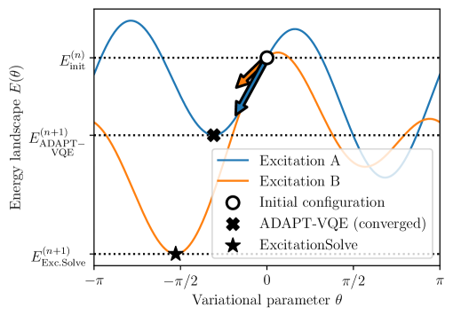
Figure 2: ADAPT-VQE vs. ExcitationSolve. We consider the selection among two excitation operator candidates A and B in the adaptive setting. In the original ADAPT-VQE approach [12], excitation A is selected based on the gradient criterion, i.e. the steepest gradient at $\theta=0$. This is then converged with a gradient descent towards a (potentially only local) minimum, typically requiring multiple gradient evaluations. ExcitationSolve chooses excitation B (despite the smaller gradient at $\theta=0$) based on the energy criterion, i.e., the attainable global energy minimum, and already initializes $\theta$ in its optimal configuration.

2.3 Multi-parameter generalization

In this section, we generalize the one-dimensional optimization to multiple dimensions, i.e. independent parameters. As illustrated in Fig. 3, this enables ExcitationSolve to potentially avoid and escape local minima in the energy landscape because a improved local or global optimum may be unveiled in a higher-dimensional space. The multi-parameter generalization can be used for both the optimization of fixed and adaptive ansätze. In the context of rotation operators, this has already been explored [9]: The energy varied in $D$ parameters is analytically described by a $D$-dimensional first-order Fourier series. Analogously, we show in Appendix B.3 that a simultaneous variation of $D$ excitation operators can be described through a $D$-dimensional second-order Fourier series. The energy landscape can thus be expressed as

$$f_{\bm{\theta}}(\bm{\theta}_{\mathcal{M}})=\bm{c}\cdot\left[\bigotimes_{i\in\mathcal{M}}\begin{pmatrix}\cos(\theta_{i})\\ \cos(2\theta_{i})\\ \sin(\theta_{i})\\ \sin(2\theta_{i})\\ 1\end{pmatrix}\right],$$ (8)

where $\bm{c}$ is a $5^{D}$-dimensional real-valued vector and $\mathcal{M}$ denotes the index set of the $|\mathcal{M}|=D$ simultaneously varied parameters. Consequently, the full reconstruction of the energy landscape requires a total of $5^{D}-1$ new energy evaluations. Once reconstructed, we can classically find the minimum of the energy landscape, our method of choice is detailed in Sec. 5.1.

The exponential number of energy evaluations in the number of parameters hinders multi-parameter ExcitationSolve from being always blindly employed. Nonetheless, it offers a useful tool when employed in the right place. Figure 3 demonstrates a perfect example of when a single application of a 2D optimization not only requires significantly fewer resources than the individual 1D optimization to converge, but also finds the global minimum instead of a local one. Generally, it can possibly set the optimizer on a more profitable path any time the 1D optimization reaches a local minimum that it cannot escape.

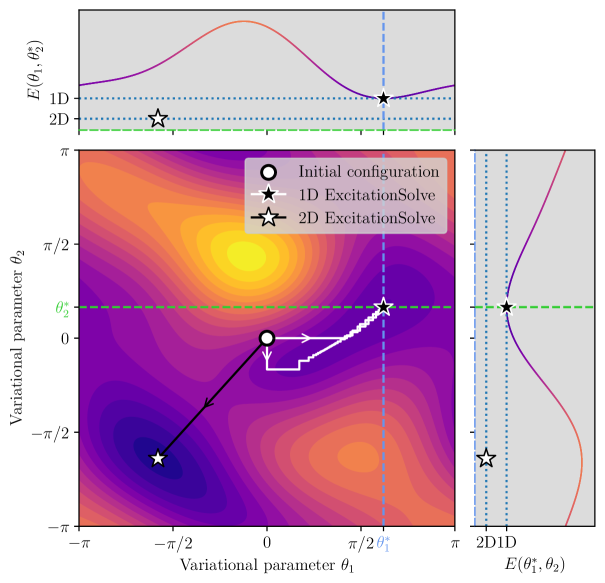
Figure 3: 1D ExcitationSolve with Coordinate Descent vs. 2D ExcitationSolve. The simultaneous optimization of two parameters can be achieved either by effectively reducing it to a 1D optimization task using coordinate descent or employing a true 2D optimization based on the energy landscape from Eq. (8). In this example, no matter which parameter is tuned first, the coordinate descent approach converges only to a local minimum. Also, this convergence takes up multiple iterations. Meanwhile, in the proper 2D case, the global reconstruction of the 2D second-order Fourier series permits an immediate jump to the global minimum.

2.4 Multiple occurrences of a single parameter

For the practical use of UCCSD, it often suffices to employ a single time step in first-order Trotterization. However, one might encounter scenarios where the expressivity of such type of ansatz is no longer sufficient and thus requires a refinement – e.g., through a higher order product formula or simply multiple time steps. In a higher order product formula, at least one or more parameters appear multiple times throughout the corresponding quantum circuit. Concerning the use of multiple time steps, there is the degree of freedom of using different parameters for every time step or sharing these parameters between multiple steps. The latter is motivated by the physical point of view of a discretized time evolution of an adiabatic process with equal time steps where the strength of the free fermionic problem, i.e. the single-excitations, is kept constant. For $S$ excitations sharing the same variational parameter $\theta$,

$$f_{\bm{\theta}}(\theta)=\sum_{s=1}^{2S}a_{s}\cos(s\theta)+\sum_{s=1}^{2S}b_{s}\sin(s\theta)+c,$$ (9)

i.e., it is a one-dimensional Fourier series of order $2S$. The $4S+1$ coefficients can be determined through $4S$ energy evaluations. This result can be straightforwardly inferred from the multi-parameter generalization from Eq. (8) by setting multiple parameters equal and reducing the trigonometric form. Equation 9 is closely related to the result for multiple occurrences of a single parameter in Rotosolve/SMO, where the energy landscape is given by a Fourier series of order $S$ with $2S+1$ coefficients [9] (cf. Sec. C.2). For a detailed derivation, refer to Appendix B.4. Note that unlike the exponential growth in energy evaluations for a multi-parameter optimization, we have a linear growth for the multi-occurrence case.

2.5 Multiple occurrences of multiple parameters

After having explored the two cases of multiple distinct parameters and multiple occurrences of a single parameter, it remains to explore the most general case: multiple occurrences of multiple parameters (different parameters may appear different number of times). The result is a straightforward conclusion of both previous results. Each unique parameter $\theta_{i}$ introduces one dimension and the order of the Fourier series in the corresponding dimension is given by the respective number of occurrences. Let $\bm{\tilde{\theta}}\subseteq\bm{\theta}$ be the subset of simultaneously varied parameters and $S_{i}$ be the number of occurrences of a parameter $\theta_{i}\in\bm{\tilde{\theta}}$. The energy landscape can then be expressed as

$$f_{\bm{\theta}}(\bm{\theta}_{\mathcal{M}})=\bm{c}\cdot\left[\bigotimes_{\theta_{i}\in\bm{\tilde{\theta}}}\left(\cos(\theta_{i}),\cos(2\theta_{i}),\dots,\cos(2S_{i}\theta_{i}),\sin(\theta_{i}),\sin(2\theta_{i}),\dots,\sin(2S_{i}\theta_{i}),1\right)^{\top}\right],$$ (10)

where $\bm{c}$ is a real-valued vector with dimension $\prod_{\theta_{i}\in\bm{\tilde{\theta}}}(4S_{i}+1)$.

3 Experiments

In this section, we assess the performance of ExcitationSolve on both fixed and adaptive ansätze. We compare it to other optimizers commonly found in VQE literature: Gradient Descent (GD), Constrained Optimization By Linear Approximation (COBYLA) [22], Adam [17], Simultaneous Perturbation Stochastic Approximation (SPSA) [23, 24] and the Broyden-Fletcher-Goldfarb-Shannon (BFGS) algorithm [18, 19, 20, 21]. The VQE is initialized with the Hartree-Fock (HF) state and parameters set to zero such that the initial energy is the HF energy $E_{\text{HF}}$. ExcitationSolve reuses previous energies, matching the four-term parameter-shift rule resources for single derivatives. To evaluate the experiments, we consider the absolute error between the VQE energy $E_{\text{VQE}}$ with respect to the exact Full Configuration Interaction (FCI) energy $E_{\text{FCI}}$, i.e., $|E_{\text{VQE}}-E_{\text{FCI}}|$. This approach helps us determine when the error falls below the desirable ${10}^{-3}\text{\,}\mathrm{Ha}$, a threshold commonly referred to as chemical accuracy. The quantum resource demand of the optimizers is tracked in the number of energy evaluations, which refers to obtaining the expectation value of the Hamiltonian and is proportional to the actual number of measurements and terms of the second-quantized Hamiltonian. The presented results are for optimizers with tuned hyperparameters. Full details on the experiments and their evaluation can be found in the Sec. 5.

3.1 Fixed ansatz (UCCSD) comparison with other optimizers

To compare the optimizers we use a fixed ansatz where the tunable parameters and the order of the parameters are exactly the same for all optimizers. The concrete choice of ansatz is the UCCSD ansatz with a single layer, constituted of all possible single and double fermionic excitations. See Sec. 5.3.2 for more details. Figure 4 presents the results where we studied the ground state energies of the molecules H2 (Fig. 4(a)), H3+ (Fig. 4(b)), LiH (Fig. 4(c)) and H2O (Fig. 4(d)), each in their equilibrium geometry according to the datasets [38, 39, 40, 41].

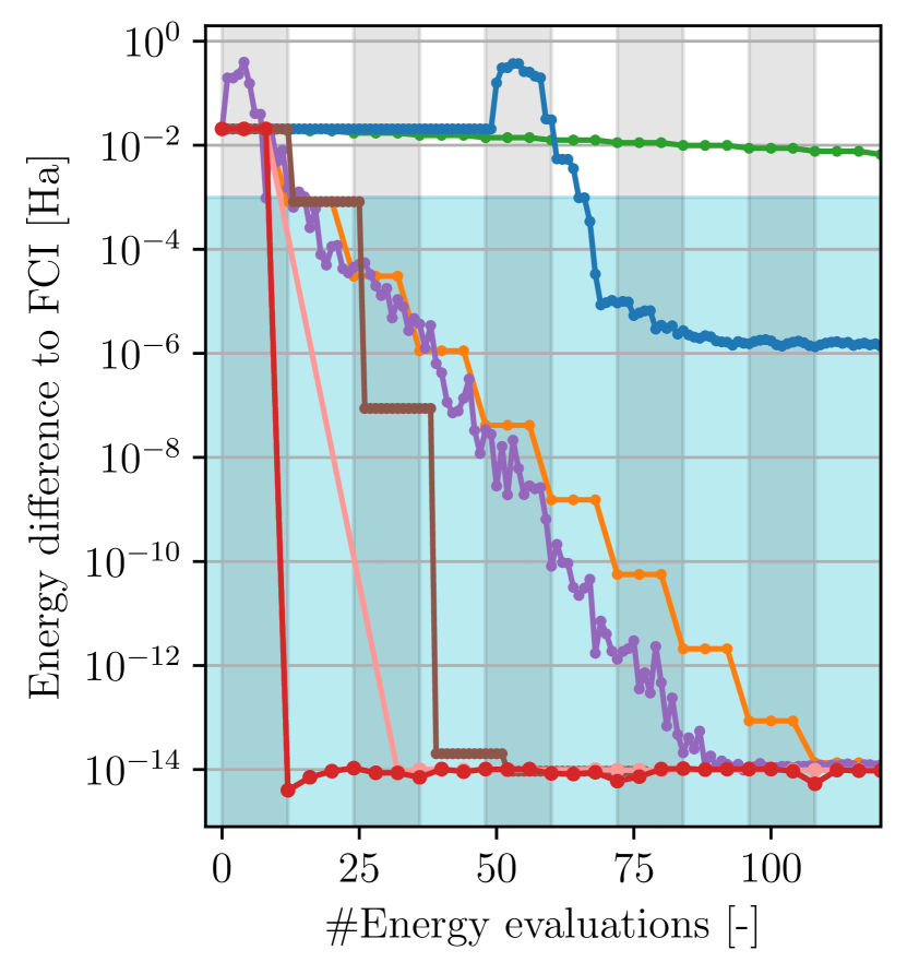
(a) H2, $4$ qubits.

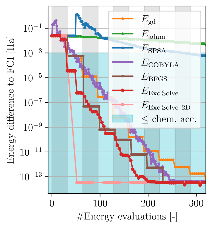
(b) H3+, $6$ qubits.

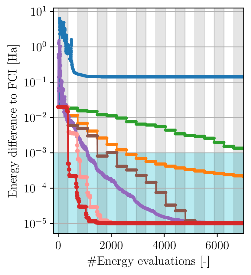
(c) LiH, $12$ qubits.

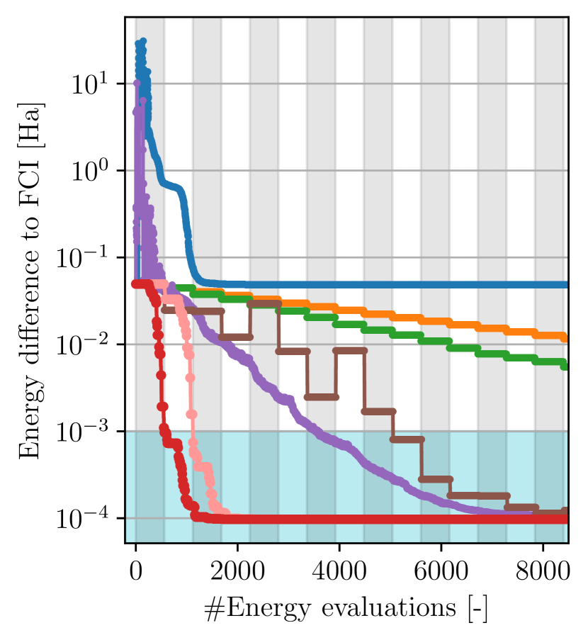
(d) H2O, $14$ qubits.

Figure 4: Comparison of optimizers for fixed UCCSD ansätze. The optimizers under consideration are ExcitationSolve (red), COBYLA (purple), Gradient descent (yellow), Adam (green), SPSA (blue) and BFGS (brown). The plots show the error of the VQE with respect to the FCI solution ${|E_{\text{VQE}}-E_{\text{FCI}}|}$ over the number of energy evaluations for the molecules a) H2, b) H3+, c) LiH and d) H2O in their respective equilibrium geometries. The light blue region signifies the chemical accuracy (${10}^{-3}\text{\,}\mathrm{Ha}$) and the alternating vertical shading marks each iteration over all parameters.

We find that ExcitationSolve does not only take fewer evaluations to reach chemical accuracy but also achieves this within a single sweep over the parameters. ExcitationSolve finds the exact ground state energy faster than all other optimizers with the most prominent speedup for larger molecules. For the H2 molecule, ExcitationSolve even converges to the FCI energy in just one VQE iteration. This efficiency is attributed to the ground state being a superposition of the Hartree-Fock state and one singly-excited state. Therefore, optimizing only the parameter in the UCCSD ansatz corresponding to the relevant single excitation is sufficient for convergence, which ExcitationSolve accomplishes optimally in a single VQE iteration. Similarly, for the H3+ molecule, ExcitationSolve with a 2D optimization strategy (see Sec. 5.3.4) converges to the FCI energy after one 2D optimization, since the FCI ground state is a superposition of the HF state and two excited states. For H2O ExcitationSolve reaches both the chemical accuracy and exact solution 7 times faster than the next best optimizer (COBYLA and BFGS, respectively). In contrast, the slowest, yet converging, optimizer (GD) takes 46 and 86 times longer to reach these accuracies. It is worth noting for larger molecules that all optimizers consistently converge with a higher error, likely due to the absence of higher-order excitations in the UCCSD ansatz and the limited expressivity of a single first-order Trotter step. As both SPSA and Adam have a very slow convergence and in some cases do not even manage to reach the chemical accuracy, we disregard them for further studies.

3.2 ADAPT-VQE

As often suggested in recent literature on variational algorithms [42], fixed ansätze may not be the way forward. We therefore probe ExcitationSolve in an adaptive setting where not only the parameters are optimized using ExcitationSolve, but also the choice of the next operator to append to the ansatz is made using the same strategy. We compare it to the original ADAPT-VQE implementation [12] where the operator selection is made by the gradient criterion and the re-optimization is performed with GD. Both are initialized in the HF state. Experimental details are reported in Sec. 5.3.3.

Figure 5 shows the convergence of the adaptive optimizations to the ground states of molecules H2, H3+, LiH and H2O in their equilibrium geometry. The total number of evaluations is composed of the evaluations to select a new operator and the evaluations to re-optimize the parameters already present in the ansatz. The former lead to plateaus, during which the energy remains unchanged. For all four molecules ExcitationSolve reaches faster convergence than ADAPT-VQE for both the chemical accuracy and the limit within the UCCSD ansatz. The reason for the faster convergence stems mainly from two key advantages that ExcitationSolve features: First, using ExcitationSolve to select new operators leads to fewer operators being added to the ansatz. This results in a shallower circuit and a cheaper re-optimization. This can be seen for the larger molecules, i.e., LiH in Fig. 5(c), where ADAPT-VQE requires 34 Operators, while ExcitationSolve only needs 30 to converge. For H2O, ADAPT-VQE needs 48 operators, while ExcitationSolve only requires 42. Note that the operator reduction only becomes significant beyond the chemical accuracy. Second, initializing the new operators with ExcitationSolve at their optimal values offers a beneficial warm start for the intermediate parameter optimization, further leading to a convergence within fewer iterations in the re-optimization of the parameters. A special case can be seen for H2 in Fig. 5(a), where only a single excitation contributes to the ground state and ExcitationSolve immediately initializes it with its optimal parameter value. The most significant reduction in energy evaluations can be observed for H2O where ExcitationSolve reaches the chemical accuracy approximately 15 times faster.

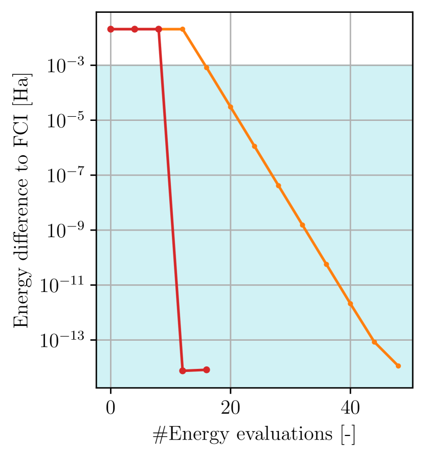
(a) H2, $4$ qubits.

(b) H3+, $6$ qubits.

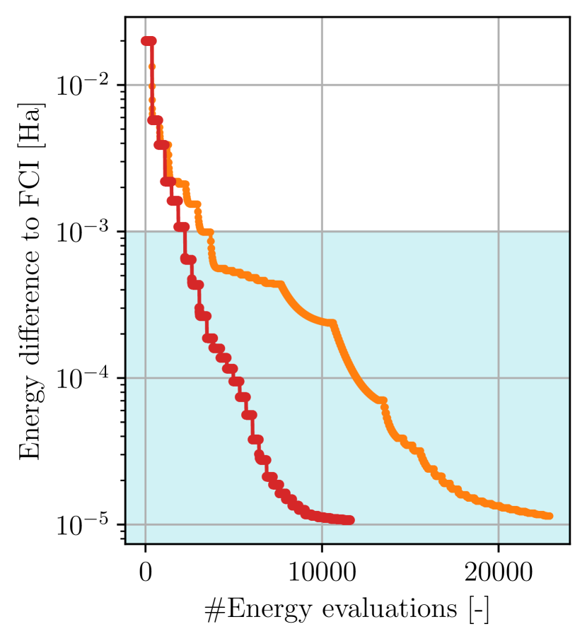
(c) LiH, $12$ qubits.

(d) H2O, $14$ qubits.

Figure 5: Comparison between ExcitationSolve and original ADAPT-VQE with the UCCSD operator pool. The plots show the error of the VQE with respect to the FCI solution ${|E_{\text{VQE}}-E_{\text{FCI}}|}$ over the number of energy evaluations for the molecules a) H2, b) H3+, c) LiH and d) H2O. The light blue region signifies the chemical accuracy (${10}^{-3}\text{\,}\mathrm{Ha}$).

3.3 Dissociation curves

We further analyze how a deviation of the HF state from the actual ground state influences the performance of ExcitationSolve compared to GD, BFGS and COBYLA when provided as the initial state in the fixed UCCSD ansatz VQE. Concretely, by varying the inter-atomic distances in the molecules, we affect how closely the HF state approximates the true ground state: The further the bond is stretched, the larger the initial HF error $|E_{\text{HF}}-E_{\text{FCI}}|$ of the HF energy $E_{\text{HF}}$ to the energy of the FCI solution $E_{\text{FCI}}$, signaling the emergence of strong correlations [43]. This HF error dependence on the bond distance for the studied molecules H2, H3+, LiH and H2O is shown in Fig. 6. For ExcitationSolve we perform both one-dimensional (1D) and two-dimensional (2D) optimization as described in Sec. 5.3.4. Implementation details can be found in Sec. 5.3.5.

Figure 6 shows how many energy evaluations are needed for different bond distances to reach convergence for each molecule. Among all molecules it becomes apparent that the higher the bond distance gets, i.e., the higher the HF error since the initial HF state deviates more from the ground state solution, the more executions of the circuit are necessary to find the ground state. We see only two exceptions: for H2 (Fig. 6(a)) the ExcitationSolve optimizer finds the ground state with a constant number of evaluations and for H3+ (Fig. 6(b)) ExcitationSolve also needs a constant number of evaluations when optimizing two parameters at the same time. These two cases are special, because (2D-)ExcitationSolve can set the parameters to the global optimum within the first VQE iteration because the ground state of H2 and H3+ are superpositions of the HF state with one and two excited states, respectively. Overall, it can be observed that ExcitationSolve outperforms the other optimizers for each bond distance. Although, the relative difference in the number of energy evaluations needed for the optimizers to reach convergence is mostly independent of the bond distance. Indeed the scaling with the bond length for the two larger molecules LiH (Fig. 6(c)) and H2O (Fig. 6(d)) is almost identical for all optimizers, with BFGS seeming least impacted by the bond distance.

Particular attention should be drawn to the two data points of the H2O dissociation curve (Fig. 6(d)) at the bond distances of $2.02\text{\,}\mathrm{\text{Å}}$ and $2.06\text{\,}\mathrm{\text{Å}}$. The convergence analysis for these data points can be inferred from Fig. 7. As detailed in Sec. 5.3.2, all parameters have been optimized in their order of appearance in the UCCSD ansatz, i.e., a fixed order. Figures 7(a) and 7(b) depict cases in which this order causes ExcitationSolve to get stuck either in local minima or extremely flat parts of the optimization landscape, thus failing to converge within a reasonable number of energy evaluations. Meanwhile, Fig. 7(a) also provides further evidence for the utility of 2D optimization, which successfully converges to the global minimum within the expressivity of the ansatz. While the 2D optimization can be utilized to escape local minima, our heuristic to simultaneously optimize the two most impacting parameters may not succeed in some rare instances. We have found one example in Fig. 7(b), where both the 1D and 2D optimizers get stuck. Fortunately, randomly shuffling the parameter order for each VQE iteration while performing solely 1D optimization achieves convergence for both cases. In the case where the 2D optimizer already converges (Fig. 7(a)), it is still notably faster than the shuffled 1D approach.

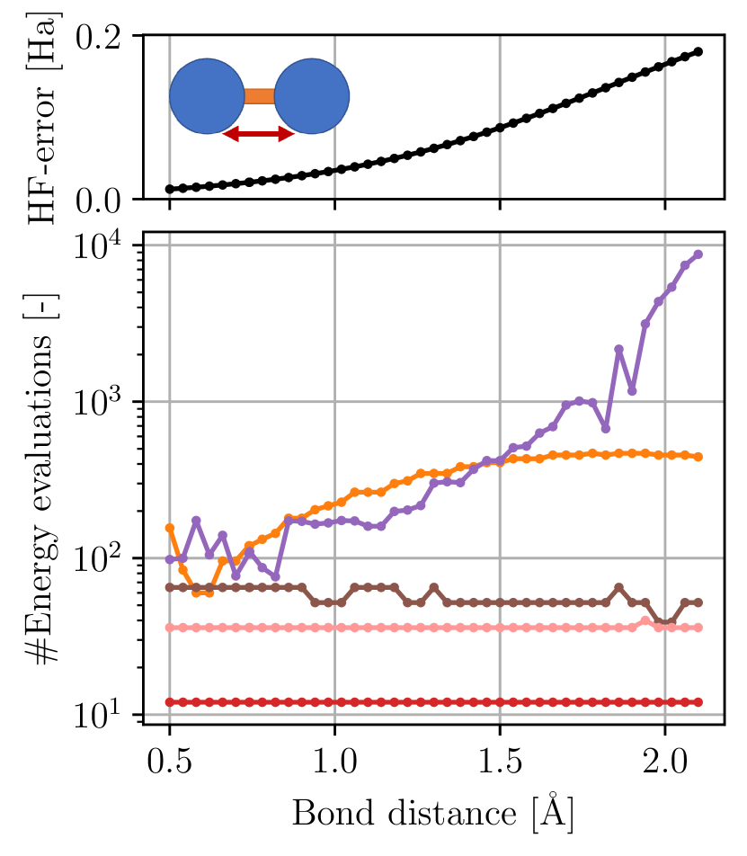
(a) H2, 4 qubits.

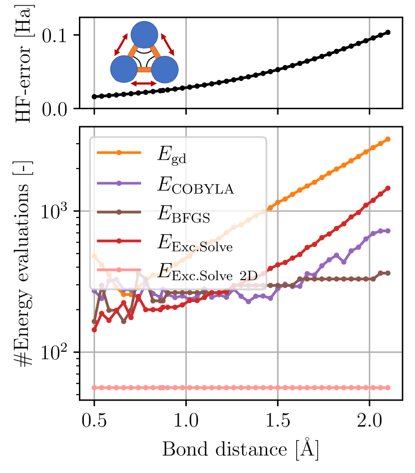
(b) H3+, $6$ qubits.

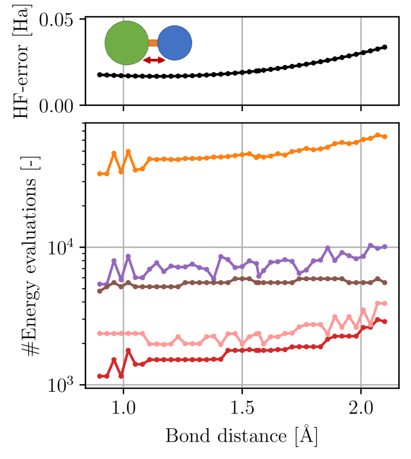
(c) LiH, 12 qubits.

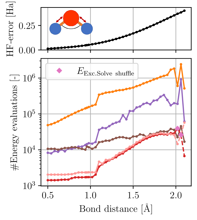
(d) H2O, 14 qubits.

Figure 6: Comparison of optimizers using fixed UCCSD ansätze for non-equilibrium geometries. Hartree-Fock (HF) error (black) and energy evaluations until VQE convergence in dependence of the bond length for optimizers ExcitationSolve (red), COBYLA (purple) and Gradient descent (yellow) for molecules a) H2, b) H3+, c) LiH and d) H2O. For H2O with high bond lengths, random shuffling of the parameter order in ExcitationSolve is additionally utilized to achieve convergence (diamond marker). The HF error is the absolute difference between the FCI energy and HF energy.

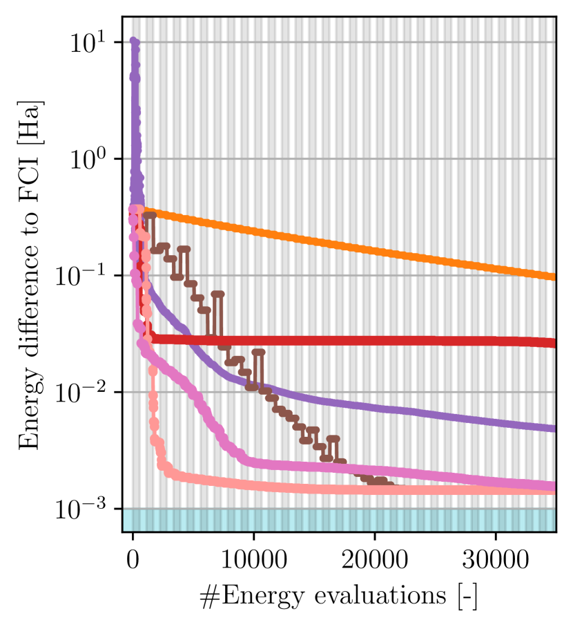
(a) H2O, 14 qubits, bond distance $2.02\text{\,}\mathrm{\text{Å}}$.

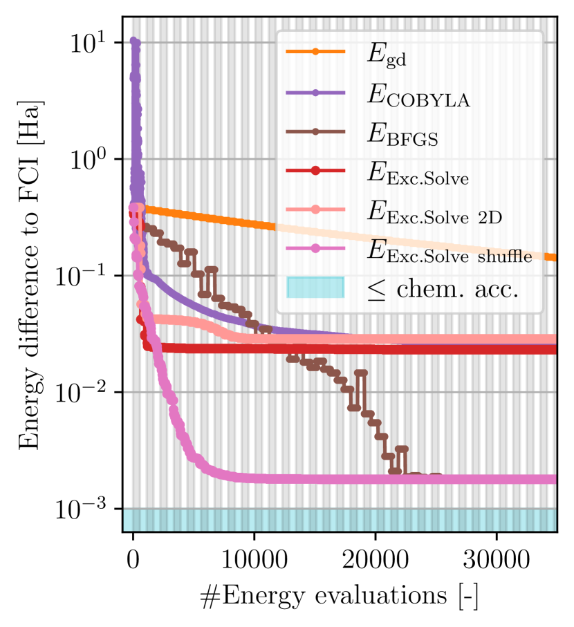
(b) H2O, 14 qubits, bond distance $2.06\text{\,}\mathrm{\text{Å}}$.

Figure 7: Optimization of H2O for two specific bond distances. The optimizers under consideration are ExcitationSolve (red), COBYLA (purple), Gradient descent (yellow) and BFGS (brown). The plots show the error of the VQE with respect to the FCI solution ${|E_{\text{VQE}}-E_{\text{FCI}}|}$ over the number of energy evaluations for the bond distances marked separately in Fig. 6(d) where parameter shuffling is used. The light blue region signifies the chemical accuracy (${10}^{-3}\text{\,}\mathrm{Ha}$) and the alternating vertical shading marks each iteration over all parameters.

3.4 Shot noise

We repeat the experiments from Sec. 3.1 with shot noise instead of exact state vector simulations. Due to the large number of shots needed to achieve chemical accuracy and the increasing computation time for larger molecules, we restrict ourselves to the molecules H2 and H3+. We perform ${10}^{7}$ shots for all optimizers and molecules in the results we show here since the overall qualitative behavior of the optimizers was rather independent of the number of shots. Implementation details can be found in Sec. 5.3.6.

Figure 8 presents the results. For optimizers that do not update parameters at each energy evaluation, we repeatedly plot the latest updated energy which results in energy plateaus which seem not affected by noise. For example, GD has these plateaus are during the calculation of the gradient. We find that the shot noise has a significant impact on all used optimizers and limits the achievable accuracy. The difference between the optimizers is less pronounced than in the state vector simulations form Sec. 3.1. Overall, the results are similar to the state vector simulations, only that the maximum achievable accuracy of every optimizer is limited by the shot noise. We see that ExcitationSolve reaches its maximum accuracy within similar number of energy evaluation as in the state vector simulations (cf. Sec. 3.1). This includes H2, where ExcitationSolve achieves its maximum accuracy within one VQE iteration. Most importantly, ExcitationSolve reaches its maximum accuracy faster than all other optimizers. With this, we note that the convergence speed of ExcitationSolve is robust against noise.

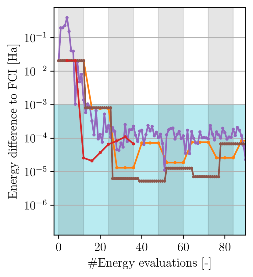
(a) H2, $4$ qubits.

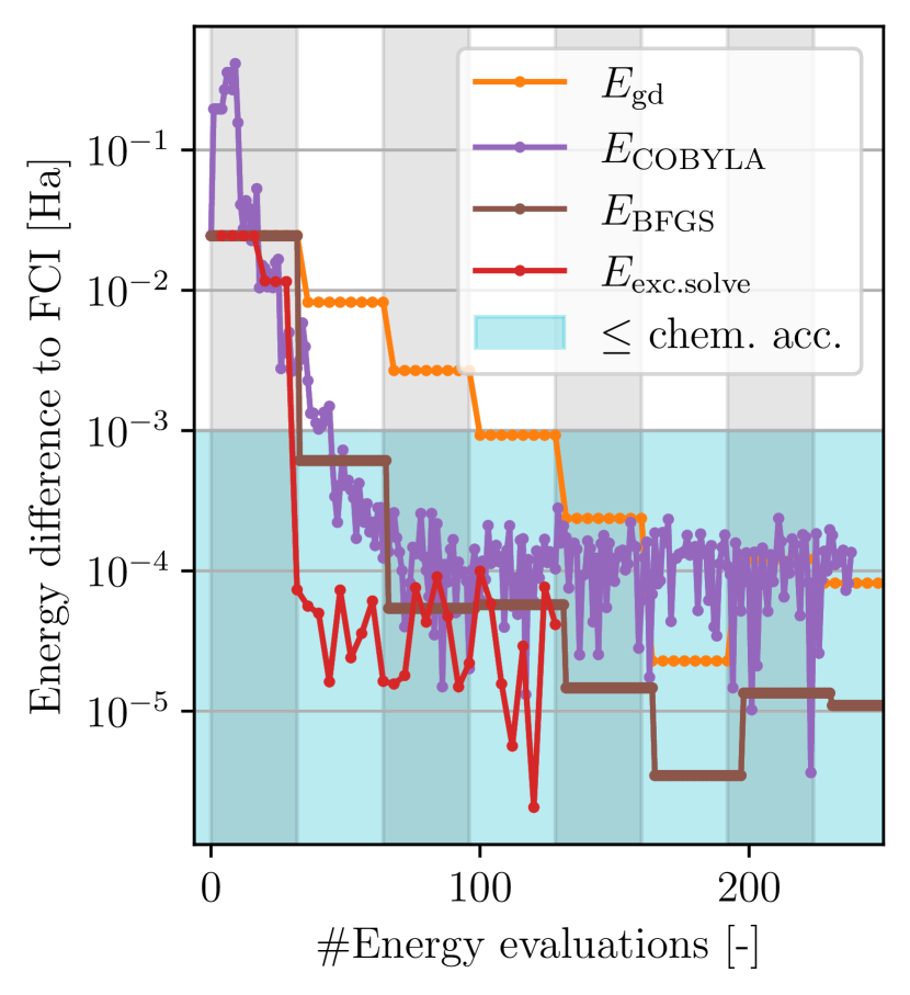
(b) H3+, $6$ qubits.

Figure 8: Comparison of optimizers under the influence of shot noise. The optimizers under consideration are ExcitationSolve (red), COBYLA (purple), Gradient descent (yellow) and BFGS (brown) with ${10}^{7}$ shots each. The plots show the error of the VQE with respect to the FCI solution ${|E_{\text{VQE}}-E_{\text{FCI}}|}$ over the number of energy evaluations for the molecules H2 (Fig. 4(a)), H3+ (Fig. 4(b)). The light blue background signifies when chemical accuracy has been reached. Vertical lines mark when one iteration over all parameters has been completed.

4 Discussion

The main motivation behind ExcitationSolve is to unite the benefits of quantum-aware optimization and physically-motivated ansätze composed of excitation operators. Due to the quantum-awareness in particular, ExcitationSolve improves over common gradient-based optimizers by informing updates globally instead of being limited to the local vicinity – without imposing any resource overhead. Specifically, reconstructing the energy landscape for a single parameter requires four energy evaluations, optimized by reusing the final minimal energy from the previous step, which matches the resource requirements for the four-term parameter-shift rule. Interestingly, the same resource-efficiency already can be observed with simpler rotations in Rotosolve. Table 1 provides a detailed comparison. Even though approaches to compute analytical gradients for excitation operators with fewer shifts exist under specific conditions [35] as presented in Sec. C.1, they are less comparable due to the reliance on additional quantum circuit dressing. In the adaptive setting, we globalize the operator selection criterion with ExcitationSolve by using the same quantum resources more effectively compared to the original gradient criterion in ADAPT-VQE [12]. We remark that any double excitation can be decomposed into a product of 8 Pauli rotations of the same angle [26]. A naive application of SMO/Rotosolve to the Pauli decomposition leads to an overestimation of the Fourier order by a factor of 4. This further worsens for higher-order excitations where SMO exponentially overestimates the Fourier order. However, the more sophisticated decomposition of excitation operators into two commuting self-inverse operators (cf. Appendix B and Ref. [35]) reveals that ExcitationSolve can be interpreted as the double-occurrence case of SMO.

Table 1: Number of energy evaluations comparison for the full single-parameter energy landscape reconstruction vs. the partial derivative via a parameter-shift rule.

	Function reconstruction		Partial derivative
	Theoretical	Effective	via parameter-shift rule
Rotations ($G^{2}=I$)	3 [8, 9]	2 [8, 9]	2 [44, 45]
Excitations ($G^{3}=G$)	5	4	4 [46]

Moreover, the relevance of ExcitationSolve is intrinsically linked to the advantages of employing physical ansätze using excitation operators. The significance of such ansätze lies in their ability to preserve essential physical quantities and symmetries. It could be argued that qubit tapering [47, 48] for hardware-efficient or problem-agnostic ansätze, i.e., composed of rotation gates, could achieve the same advantages, however qubit tapering conserves the particle numbers and spin symmetries only up to their parity. Note that ExcitationSolve natively handles excitation operators, independent of the actual decompositions, fermion-to-qubit mappings and simplifications of the ansatz to the quantum circuit. In addition, organizing the parameters in a problem-informed way via such physical excitation operators could lead to a simpler, more suggestive optimization landscape as it has been observed in other contexts [49]. Alternatively, the choice of physically-motivated ansätze can be interpreted as encoding an inductive bias, and, hence, could effectively restrict the exponentially growing underlying Hilbert space. This potentially counteracts the emergence of so-called barren plateaus, which would obstruct the practical use in realistic, large-scale problem sizes [42].

Our experimental results demonstrate multiple advantages of ExcitationSolve over previous state-of-the-art optimizers, including gradient descent (GD), COBYLA [22], Adam [17], SPSA [23, 24], and BFGS [18, 19, 20, 21]: Firstly, for a fixed UCCSD ansatz ExcitationSolve generally takes fewer iterations to converge to the ground state than any other tested optimizer. How significant the advantage is depends on the molecule. Secondly, ExcitationSolve has no hyperparameters that need to be tuned and needs no calibration. Thirdly, in an adaptive setting, like ADAPT-VQE [12], ExcitatonSolve can be used to choose the next operator to append based on its highest impact on the energy value outperforming the locally informed selection such as the original ADAPT-VQE gradient criterion. The newly picked operator is also already initialized in its optimal parameter value, which significantly warm-starts the intermediate optimization of all present parameters before extending the ansatz further.

While ExcitationSolve offers promising features, it faces certain challenges, such as the potential for getting trapped in a local minimum. This issue becomes particularly significant for larger molecules, where the proliferation of local minima poses a critical challenge. To address this, we proposed a multi-dimensional extension of ExcitationSolve, though this approach introduces new complexities, such as increased computational cost, as the number of evaluations grows exponentially with the number of parameters. Moreover, determining which parameters to pair for optimization is complex due to the combinatorial nature of the problem. One effective heuristic is to pair operators with the strongest impact from single-parameter optimization, as demonstrated with the H3+ molecule. In the case of H2O, we observe that this heuristic is not always sufficient to avoid local minima. Fortunately, we find that parameter shuffling provides another, complementary approach to avoid local minima – and unlike the 2D optimizer does not even require additional computational effort. Identifying strong heuristics for beneficial parameter orderings and for how and when multi-parameter optimization can be employed to navigate the energy landscape faster and more reliably remains an area for future investigation.

5 Methods

5.1 Classical minimization of analytic energy reconstructions

After reconstructing the energy function, in order to determine the global minimum in the single parameter (or set of parameters) classically, we suggest the utilization of the following approaches.

Single-parameter case (companion-matrix method).

The first important realization is that the derivative of the finite Fourier series determining the energy function in one parameter as in Eq. (3), is again a Fourier series of the same order, i.e., $\tfrac{d}{d\theta}b_{s}\sin(s\theta)=b_{s}s\cos(s\theta)$, $\tfrac{d}{d\theta}a_{s}\cos(s\theta)=-a_{s}s\sin(s\theta)$ and zero constant. Of this derivative function we can determine the zeros and evaluate the analytic energy function (classically) at these points. The smallest of the resulting energy values must be the global minimum.

Finding the zeros of the derivative can be achieved efficiently through the so-called companion-matrix method. In the following we provide a brief review of this technique introduced in Ref. [50] for a general (finite) Fourier series. Note that the constant term $c=0$ as we deal with minima, i.e., zeros of derivatives:

$$f(\theta)=\sum_{s=1}^{S}a_{s}\cos(s\theta)+\sum_{s=1}^{S}b_{s}\sin(s\theta).$$ (11)

By employing the Euler identity, this finite Fourier series may be recast into the complex form

$$f(\theta) =\sum_{s=1}^{S}\left(\frac{a_{s}-ib_{s}}{2}e^{is\theta}+\frac{a_{s}+ib_{s}}{2}e^{-is\theta}\right)$$

$$=e^{-iS\theta}\sum_{s=1}^{S}\left(\frac{a_{s}-ib_{s}}{2}e^{i(S+s)\theta}+\frac{a_{s}+ib_{s}}{2}e^{i(S-s)\theta}\right)$$

$$=e^{-iS\theta}\left(\sum_{s=S+1}^{2S}\frac{a_{s-S}-ib_{s-S}}{2}e^{is\theta}+\sum_{s=0}^{S-1}\frac{a_{S-s}+ib_{S-s}}{2}e^{is\theta}\right).$$ (12)

By introducing the transformation $z=e^{i\theta}$, we rewrite the Fourier series as

$$f(\theta)=\frac{z^{-S}}{2}\sum_{s=0}^{2S}h_{s}z^{s}=:\frac{z^{-S}}{2}h(z),$$ (13)

where

$$h_{s}=\begin{cases}a_{S-s}+ib_{S-s},&s=0,1,\dots,S-1\\ 0,&s=S\\ a_{s-S}-ib_{s-S},&s=S,S+1,\dots,2S.\end{cases}$$ (14)

and $h(z)$ is referred to as the associated polynomial. Note that the problem of finding the real zeros of $f(\theta)$ has now been transformed to the task of determining the zeros of $h(z)$ on the complex unit circle. To solve for the roots of the associated polynomial, the $2S\times 2S$ companion matrix/Frobenius matrix $B$ is constructed with the component in the $s$-th row and $t$-th column

$$B_{st}=\begin{cases}\delta_{s,t-1},&s=1,2,\dots,2S-1\\ -\frac{h_{t-1}}{a_{S}-ib_{S}},&s=2S,\end{cases}$$ (15)

where $\delta$ denotes the Kronecker delta. The characteristic polynomial of the companion matrix is precisely the associated polynomial from before. In the case of ExcitationSolve, where $S=2$, the companion matrix takes the form

$$B=\begin{pmatrix}0&1&0&0\\ 0&0&1&0\\ 0&0&0&1\\ -\frac{a_{2}+ib_{2}}{a_{2}-ib_{2}}&-\frac{a_{1}+ib_{1}}{a_{2}-ib_{2}}&0&-\frac{a_{1}-ib_{1}}{a_{2}-ib_{2}}\end{pmatrix}$$ (16)

The roots $\theta_{k}$ of $f$ are then obtained as

$$\theta_{k}=\text{arg}(z_{k})+2\pi m-i\log(|z_{k}|),$$ (17)

where $z_{k}$ is the $k$-th eigenvalue of $B$ and $m$ is some integer. Here, it becomes clear that $\theta_{k}$ is real iff $z_{k}$ lies on the complex unit circle.

Multi-parameter case (Nyquist initialization and local optimization).

In the case of an analytic energy function in multiple parameters to be optimized as in Eq. (8), we can no longer employ the companion-matrix method.

One naive way to find the minimum of a multiple-dimensional energy landscape lies in rasterizing of the parameter space. For low dimensions, such a brute-force evaluation can be easily performed on a classical computer (keep in mind that the energy function has already been faithfully reconstructed and can be evaluated at arbitrary positions in parallel). For this type of approach, however, the precision of the result is limited by the resolution of the grid, which is not desirable as the precision then depends precisely on the position of the minimum and cannot be assumed to be constant.

Inspired by the Nyquist-Shannon sampling theorem [51], we conjecture that it is sufficient to evaluate the energy function with a lattice spacing of $\Delta=2\pi/(2\omega_{\mathrm{max}}+1)$, where $\omega_{\mathrm{max}}=2S$ is the highest frequency in the system along an $S$-fold occurring parameter, i.e., we sample with at least twice the highest frequency of the system (Nyquist frequency), which is $2\omega_{\mathrm{max}}+1$ equidistant samples within the period. Each of those lattice points is then taken as an initial guess for a local optimization scheme such as gradient descent. This can be implemented on classical hardware very efficiently for the following reasons. Firstly, all runs for the different initial guesses can be performed in parallel. Secondly, since the function to be minimized is known analytically, analytical gradients are also readily available. Thirdly, through an optimal gradient descent step size $\alpha$, the convergence is guaranteed and the convergence speed can be improved significantly with $\alpha=1/L$ where $L$ denotes a Lipschitz constant of the gradient [52], which can be determined given the analytic form as a multi-dimensional Fourier series. Bear in mind that, while this technique performs much more efficiently and precisely than a naive high-resolution grid evaluation, its computational costs still scales exponentially in the number of (different) parameters.

5.2 Reconstruction strategies for noise robustness

As the analytic energy landscape is resembled by a second-order Fourier series as in Eq. (3), five energy evaluations set the minimum requirement to uniquely determine the five coefficients. However, the energy landscape reconstruction in ExcitationSolve can be readily extended beyond five energy evaluations. Assuming that the energy evaluations are inexact (e.g. due to device- or shot-noise), this approach can make ExcitationSolve more robust against noise.

The then overdetermined linear equation system can then be solved in two ways: Using the least-squares method or a discrete Fourier transform. From a statistical perspective, the least-squares method is solving the regression problem in a second-order Fourier basis expansion [53]. Then, in terms of maximum-likelihood optimality, the least-squares estimation yields the optimal result under a normally distributed noise assumption [54]. This assumption is approximately fulfilled for pure shot-noise with practical shot numbers [55], yet only sometimes observed for hardware noise [56]. The discrete Fourier transform truncated at the second order could be utilized because higher frequencies cannot be contained in the energy landscape as in Eq. (3) but are solely subject to noise. Both approaches can in fact be seen as equivalent if the parameter-shifts are equidistant, which is necessary for the Fourier transform and generally suggested [57]. The equivalence can be supported by the least-squares guarantee when solving the regression problem [54] and the best approximation principle of the truncated Fourier transform [58]. Both arguments are made under the $L^{2}$ norm and exhibit the geometrical interpretation of orthogonal projections on the feasible function space [59, 58].

From a practical perspective, the possibility of using more than five energy values raises the following question: Given a fixed shot budget $T$, should we rather spend more shots per energy evaluation or query more energy values for the best energy reconstruction? The corresponding variance of the energy estimate when allocating $t$ shots per evaluation for any parameter position $\theta_{j}\in[-\pi,\pi]$ is given by ${(\Delta H)^{2}}/{t}$ [55] where (one-shot) observable variance $(\Delta H)^{2}$ depends on the prepared quantum state and, consequently, on the choice of parameters $\bm{\theta}$. To simplify the subsequent discussion, we assume $(\Delta H)^{2}$ to be constant and incorporate it into a proportionality constant. For the total shot budget $T$, we perform $t=T/N$ shots for each of the $N$ energy evaluations. Then, each energy evaluation is estimated with a noise variance of $\sigma^{2}\sim\tfrac{1}{T/N}$, which leads to an average variance of these $N$ estimates of $\sigma^{2}_{T}\sim\sigma^{2}/N$. Therefore, this average estimate variance becomes $\sigma^{2}_{T}\sim 1/T$, i.e., inverse-proportional to the total shot budget $T$ and, importantly, independent of $N$. In conclusion, the distribution of shots per energy evaluation under a fixed shot budget will not quantitatively change the information extracted from the quantum computer and, thus, does not impact the quality of the reconstruction. On the other hand, if we relax the assumption of a constant observable variance $(\Delta H)^{2}$, which is certainly expected in practice, we cannot make general statements about a trade-off between the shot count and number of energy evaluations. Otherwise, $(\Delta H)^{2}$ must be known (again of a finite Fourier series form), however, its estimation could pose a significant challenge in practice due to the likely high number of terms in $H^{2}$.

5.3 Experimental setup

The majority of the experiments were implemented in Python using the quantum computing framework Pennylane [60].

5.3.1 Hyperparameter tuning and calibration

For both GD and Adam we perform a hyperparameter tuning for the step size. For Adam we set the momentum parameters to $\beta_{1}=$0.9$$ and $\beta_{2}=$0.99$$ and keep them fixed for every step size. We consider the following step sizes: $1\times 10^{n}$ and $5\times 10^{n}$ for $n\in\{-4,-3,-2,-1,0\}$. Figure 9 in the appendix shows the performance of the investigated step sizes. SPSA also has two tunable hyperparameters, the learning rate and the perturbation for the gradient approximation. We use the SPSA implementation in qiskit [61] and use its calibration function to tune both hyperparameters before starting the VQE optimization at the constant cost of $50$ energy evaluations [62]. To account for this calibration phase, we plot the Hartree-Fock energy for the first $50$ SPSA energy evaluations for each molecule. We find that tuning the hyperparameters of COBYLA has negligible impact on the convergence and, therefore, use the default parameters of the SciPy implementation [63]. For the BFGS optimizer we used the SciPy implementation which has no hyperparameters. We emphasize again that ExcitationSolve has no hyperparameters that need to be tuned.

5.3.2 Fixed UCCSD ansatz

We choose the UCCSD ansatz in its first Trotter-approximation and use the STO-3G basis set as provided by the Pennylane datasets [38, 39, 40, 41] and the Jordan-Wigner (JW) mapping [31]. The system is initialized in the HF state and zero parameters. In each VQE iteration, all parameters are optimized in the order in which they appear in the ansatz (first the double-, then the single-excitations), unless explicitly stated otherwise. The step sizes for each molecule determined through hyperparameter tuning are listed in Table 2.

Table 2: Optimal step sizes for the GD and Adam optimizers.

	GD	Adam
H2	1	0.01
H3+	1	0.01
LiH	0.5	0.01
H2O	0.05	0.005

5.3.3 Adaptive Ansatz

The experimental setting follows the one of the experiments with the fixed UCCSD ansatz, except that the optimization starts with an empty ansatz. Instead, the fermionic excitation operators from the UCCSD ansatz in its first Trotter-approximation constitute the operator pool for ADAPT-VQE. We employ pool draining, which means that once an operator was selected to extend the ansatz, it is removed from the pool and cannot be used again – thus, the number of ADAPT steps is limited by the size of the pool. We also set a threshold that no more operators are attached when their impact is less than a set threshold value. This value has to be tuned for each molecule individually to achieve optimal convergence. For ExcitationSolve the threshold is an absolute energy difference, for ADAPT-VQE the threshold is a gradient. The chosen values are shown in Table 3.
After each ADAPT step, all parameters are re-optimized until convergence, the corresponding thresholds can again be found in Table 3. ExcitationSolve follows the parameter order in which they were attached. The step sizes for GD in the original ADAPT-VQE counterpart are the same as for the fixed ansatz listed in Table 2.

Table 3: Optimal threshold values in $\mathrm{Ha}$ for operator selection and VQE convergence. For ExcitationSolve the threshold is an absolute energy difference between evaluations, for GD the threshold is a gradient.

	ExcitationSolve		ADAPT-VQE
	VQE	operator selection	VQE	operator selection
H2	$10^{-6}$	$10^{-6}$	$10^{-13}$	$10^{-13}$
H3+	$10^{-6}$	$10^{-6}$	$10^{-13}$	$10^{-8}$
LiH	$10^{-7}$	$10^{-7}$	$10^{-7}$	$10^{-7}$
H2O	$10^{-6}$	$10^{-6}$	$10^{-8}$	$10^{-8}$

5.3.4 ExcitationSolve 2D optimization

In the 2D optimization variant of ExcitationSolve, we first perform a sweep over all parameters and rank them based on the difference between their global energy minimum and the Hartree-Fock (HF) energy. This assesses the immediate impact of the operators on improving the HF error. During this initial sweep no parameter values are updated. The top two most impactful parameters are first simultaneously optimized in each VQE iteration, as explained in Section 2.3, while afterwards all other parameters are optimized independently, i.e., using standard 1D ExcitationSolve. In the evaluation and plotting of the experiments, the initial sweep is included in the total number of energy evaluations, treated equivalently to a VQE iteration in the 1D ExcitationSolve optimization.

5.3.5 Dissociation experiments

We use a fixed UCCSD ansatz in its first Trotter-approximation with fermionic excitations with a Hamiltonian representation in the STO-3G basis set, using all available bond lengths in the Pennylane datasets [38, 39, 40, 41]. The initial state is again the HF state for all configurations. The hyperparameters for the used optimizers are the same as in Section 3.1. Convergence is defined as approaching the FCI energy up to a certain threshold. As not all molecules converge to the same accuracy, the threshold is specified for each molecule individually depending on the lowest accuracy achieved over all bond lengths (see Table 4).

Table 4: Convergence threshold values for each molecule

	Threshold
H2	$5.78E{-12}\text{\,}\mathrm{Ha}$
H3+	$2.64E{-13}\text{\,}\mathrm{Ha}$
LiH	$2.17E{-5}\text{\,}\mathrm{Ha}$
H2O	$2.27E{-3}\text{\,}\mathrm{Ha}$

5.3.6 Shot noise simulations

The experimental setup is identical to that of the fixed UCCSD ansatz experiments, except that a finite number of shots is used, resulting in energy evaluations being based on estimates rather than exact values. We find that when defining a fixed shot budget, changing the number of shots per energy evaluation or using more energy values for reconstructing the energy landscape has negligible impact on the convergence of ExcitationSolve. Therefore, we use $5$ energy values. For COBYLA and BFGS their default termination schemes in the respective scipy implementations are used. The optimization of gradient descent and ExcitationSolve was automatically stopped if the energy after the current VQE iteration was larger than the energies after the last two VQE iterations.

6 Acknowledgments

We thank Jakob S. Kottmann and David Wierichs for fruitful discussions. We would also like to thank Thomas Plehn and Gabriel Breuil for helpful comments on the manuscript. This project was made possible by the DLR Quantum Computing Initiative and the Federal Ministry for Economic Affairs and Climate Action; https://qci.dlr.de/quanticom (J.J., T.N.K., M.H., and E.S.). We further acknowledge the NSERC CREATE in Quantum Computing Program, grant number 543245 (J.J.).

7 Author contributions

J.J. initiated and managed the project, and devised the main concepts and initial proofs. T.N.K. worked out the large majority of the theoretical proofs. All authors conceived and planned the experiments. J.J. implemented the methods, while M.H., and E.S. wrote the simulation code. M.H. and E.S. carried out the experiments. All authors analyzed the data and contributed to the interpretation of the results. All authors contributed to writing the manuscript, with J.J. and T.N.K. leading the effort.

Appendix A Supplementary experimental results and analyses

The following material provides further details and insight into the performed experiments and analysis of ExcitationSolve.

A.1 Hyperparameter tuning results

As found in preliminary experiments, the performance of the gradient-based optimizers is susceptible to we well-tuned step size hyperparameter. We consider the following step sizes: $1\times 10^{n}$ and $5\times 10^{n}$ for $n\in\{-4,-3,-2,-1,0\}$. The detailed results for the different runs for the performed hyperparameter tuning as outlined in Sec. 5.3.1 are presented here in Fig. 9.

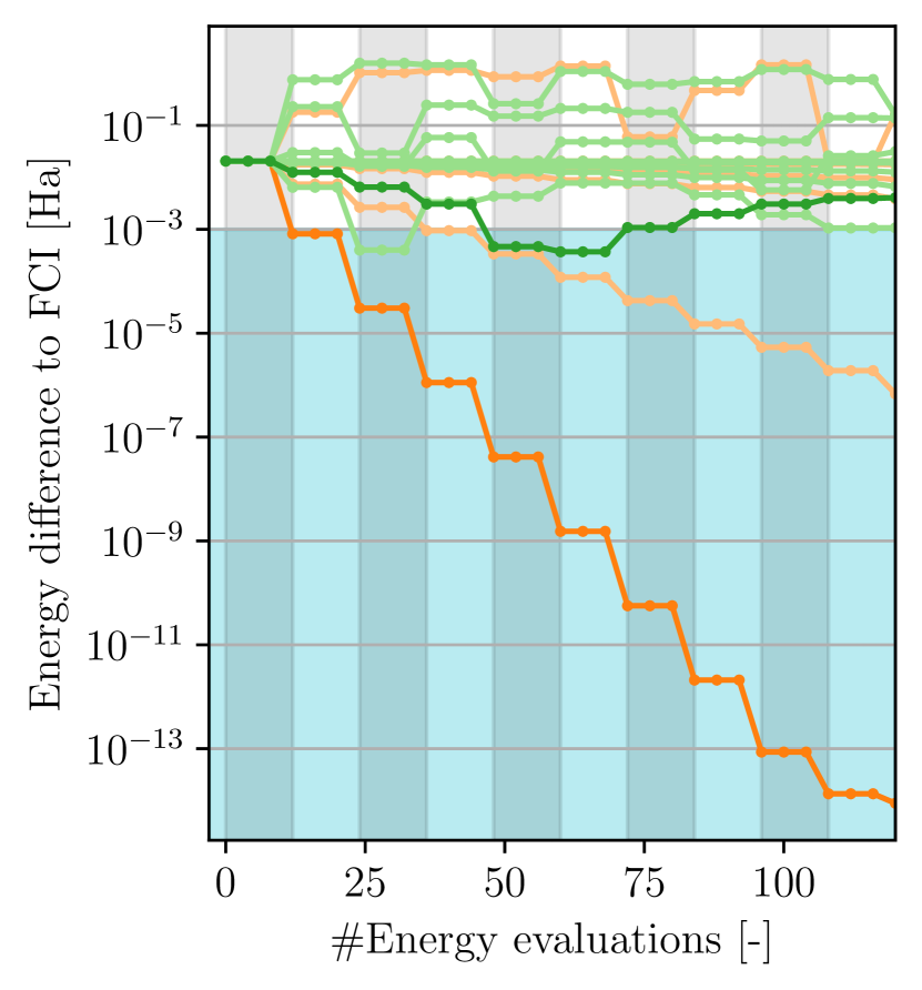
(a) H2, 4 qubits.

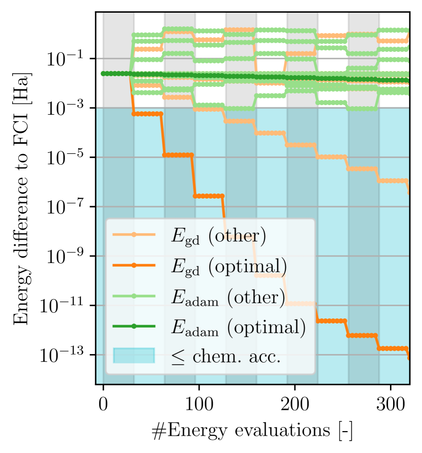
(b) H3+, 6 qubits.

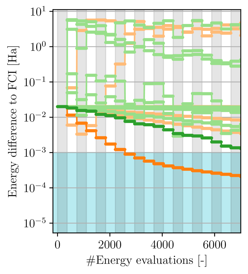
(c) LiH, 12 qubits.

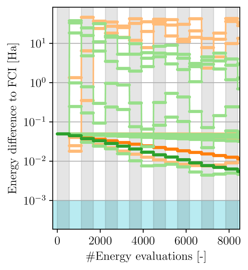
(d) H2O, 14 qubits.

Figure 9: Comparison of optimizer step sizes. The optimizers under consideration are Gradient descent (yellow) and Adam (green). The plots show the error of the VQE with respect to the FCI solution ${|E_{\text{VQE}}-E_{\text{FCI}}|}$ over the number of energy evaluations for all tested step sizes. The optimal step size is highlighted. The light blue region signifies the chemical accuracy (${10}^{-3}\text{\,}\mathrm{Ha}$) and the alternating vertical shading marks each iteration over all parameters.

A.2 ADAPT-VQE resource comparison

Figure 10 displays how well ExcitationSolve and ADAPT-VQE converge to the ground state given a fixed amount of computational resources for the following molecules: H2, H3+, LiH. On the x-axis is the number of operators that have been attached to the ansatz. As we employ pool-draining, this number is limited by the number of operators in the pool for each molecule. The y-axis shows how often each parameter is re-optimized after each ADAPT-step. Here the threshold is set by a convergence criteria that the change in energy between re-optimizations must be larger than $E{-6}\text{\,}\mathrm{Ha}$. An analysis for H2O has been spared due to exceeding reasonable computational time.

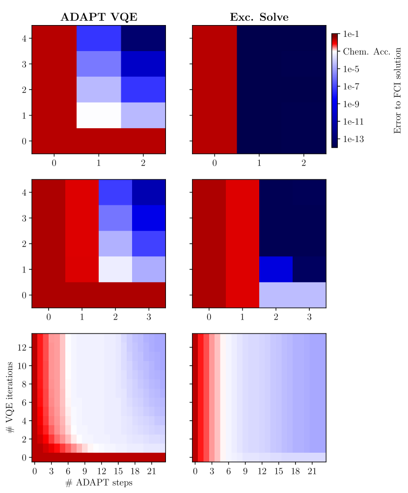
Figure 10: ExcitationSolve (right) in an adaptive setting compared with the original ADAPT-VQE (left) based on GD for molecules (top to bottom) H2, H3+, LiH. On both axes are the resources spent on the calculation: The number of ADAPT steps signals how many operators have been appended to the ansatz, the number of VQE iterations indicates how often each of the parameters has been optimized in each ADAPT step. The color code signals how close the result is to the exact FCI solution.

Apart from the overall faster convergence that can be inferred from Fig. 5, ExcitationSolve particularly shines regarding the initialization/warm-start strategy: ExcitationSolve initializes the newly attached operator in its optimal configuration, so it immediately has an impact without any additional energy evaluation overhead. In contrast, the standard ADAPT-VQE initialization sets the parameter to zero, which does not have any direct impact on the energy but heavily relies on the subsequent VQE re-optimization. Indeed, we find that while the GD based algorithm always needs to re-optimize its parameters, further VQE iterations rarely have a substantial impact when using ExcitationSolve.

Appendix B Proofs

B.1 Analytic energy function in single parameter

We present three proofs that show that the energy function in Eq. (1) has the analytical form of a second-order Fourier series as in Eq. (3). First, a constructive proofs is presented, which also shows the explicit connection of the coefficients $a_{1},a_{2},b_{1},b_{1},c$ in Eq. (3) and (expectation values of) observables of variationally prepared states.

Proof.

The excitation operators $U(\theta)$ as defined in Eq. (2) have a Hermitian generator $G$ with the property $G^{3}=G$. The exponential series simplifies to the Euler formula

$$U(\theta)=\exp(-i\theta G)=I+\left(\cos(\theta)-1\right)G^{2}-i\sin(\theta)G.$$ (18)

because $G^{3}=G$ [46]. This property can also be motivated through a hidden SU(2) symmetry associated with operators of the type $G^{3}=G$, as already studied for excitation operators in Refs. [64, 65, 66, 67]. When varying the parameter $\theta_{j}$ of a single excitation operator, while leaving all the other parameters $\theta_{i<j}$ and $\theta_{i>j}$ of preceding and succeeding excitation operators, respectively, in the circuit $U(\bm{\theta})=\prod_{k}U(\theta_{k})$ fixed. Hence, these operators can be subsumed in the input state

$$\left(\prod_{i<j}U(\theta_{i})\right)\ket{\psi_{0}}=:\ket{\psi^{\prime}}$$ (19)

and observable

$$\left(\prod_{i>j}U(\theta_{i})\right)^{\dagger}H\left(\prod_{i>j}U(\theta_{i})\right)=:H^{\prime},$$ (20)

respectively, allowing us to re-phrase the energy function of Eq. (1) through the following expectation value

$$f_{\bm{\theta}}(\theta)=\braket{\psi^{\prime}}{U^{\dagger}(\theta)H^{\prime}U(\theta)}{\psi^{\prime}}.$$ (21)

The dependence of the state $\ket{\psi^{\prime}}$ and observable $H^{\prime}$ on the remaining parameters are omitted, as well as the index of the varied parameter $\theta_{j}=\theta$, for the sake of clarity. Inserting now the Euler formula in Eq. (18) into Eq. (21) yields

$$f_{\bm{\theta}}(\theta) =\Braket{\left(I+\left(\cos(\theta)-1\right)G^{2}+i\sin(\theta)G\right)H^{\prime}\left(I+\left(\cos(\theta)-1\right)G^{2}-i\sin(\theta)G\right)}$$ (22)

$$=\phantom{+}\Braket{\left\{H^{\prime},G^{2}\right\}}\left(\cos(\theta)-1\right)+\Braket{G^{2}H^{\prime}G^{2}}\left(\cos(\theta)-1\right)^{2}$$

$$\mathrel{\phantom{=}}+\Braket{i\left[GH^{\prime}G,G\right]}\left(\cos(\theta)-1\right)\sin(\theta)$$

$$\mathrel{\phantom{=}}+\Braket{i\left[G,H^{\prime}\right]}\sin(\theta)+\Braket{GH^{\prime}G}\sin^{2}(\theta)$$

$$\mathrel{\phantom{=}}+\Braket{H^{\prime}}$$ (23)

$$=\phantom{+}\left(\Braket{\left\{H^{\prime},G^{2}\right\}}-2\Braket{G^{2}H^{\prime}G^{2}}\right)\cos(\theta)$$

$$\mathrel{\phantom{=}}+\Braket{i\left[GH^{\prime}G,G\right]}\sin(\theta)\cos(\theta)$$

$$\mathrel{\phantom{=}}+\left(\Braket{i\left[G,H^{\prime}\right]}-\Braket{i\left[GH^{\prime}G,G\right]}\right)\sin(\theta)$$

$$\mathrel{\phantom{=}}+\Braket{G^{2}H^{\prime}G^{2}}\cos^{2}(\theta)$$

$$\mathrel{\phantom{=}}+\Braket{GH^{\prime}G}\sin^{2}(\theta)$$

$$\mathrel{\phantom{=}}+\Braket{H^{\prime}}-\Braket{\left\{H^{\prime},G^{2}\right\}}+\Braket{G^{2}H^{\prime}G^{2}},$$ (24)

where all expectation values above are to be understood with respect to $\ket{\psi^{\prime}}$, i.e., $\braket{\cdot}=\braket{\psi^{\prime}}{\cdot}{\psi^{\prime}}$. Considering the three trigonometric identities, Pythagorean trigonometric identity $\cos^{2}(\theta)+\sin^{2}(\theta)=1$, double-angle-formula $\sin(\theta)\cos(\theta)=\sin(2\theta)/2$, and power-reduction-formula $\sin^{2}(\theta)=\left(1-\cos(2\theta)\right)/2$, we obtain

$$f_{\bm{\theta}}(\theta) =\phantom{+}\underbrace{\left(\Braket{\left\{H^{\prime},G^{2}\right\}}-2\Braket{G^{2}H^{\prime}G^{2}}\right)}_{=\,a_{1}}\cos(\theta)$$

$$\mathrel{\phantom{=}}+\underbrace{\tfrac{1}{2}\left(\Braket{G^{2}H^{\prime}G^{2}}-\Braket{GH^{\prime}G}\right)}_{=\,a_{2}}\cos(2\theta)$$

$$\mathrel{\phantom{=}}+\underbrace{\left(\Braket{i\left[G,H^{\prime}\right]}-\Braket{i\left[GH^{\prime}G,G\right]}\right)}_{=\,b_{1}}\sin(\theta)$$

$$\mathrel{\phantom{=}}+\underbrace{\tfrac{1}{2}\Braket{i\left[GH^{\prime}G,G\right]}}_{=\,b_{2}}\sin(2\theta)$$

$$\mathrel{\phantom{=}}+\underbrace{\Braket{H^{\prime}}-\Braket{\left\{H^{\prime},G^{2}\right\}}+\tfrac{1}{2}\left(\Braket{GH^{\prime}G}+3\Braket{G^{2}H^{\prime}G^{2}}\right)}_{=\,c}.$$ (25)

Recognizing that Eq. (25) precisely matches the form of a second-order Fourier series for the energy function in a single parameter as in Eq. (3) concludes the proof. ∎

Second, we provide an alternative proof of this connection between Eq. (1) and Eq. (3), given the theory of general parameter-shift rules [25], which links the eigenvalues of $G$ to the frequencies present in the energy function.

Proof (alternative I).

Given the eigenvalues $\{\omega_{i}\}$ of the Hermitian generator $G$ of a single parameterized operator $U(\theta)=\exp(i\theta G)$, Ref. [25] determines that the energy function Eq. (1) can be written in the form of a finite Fourier series

$$f_{\bm{\theta}}(\theta_{j})=a_{0}+\sum_{\ell=1}^{R}a_{\ell}\cos\left(\Omega_{\ell}\theta_{j}\right)+\sum_{\ell=1}^{R}b_{\ell}\sin\left(\Omega_{\ell}\theta_{j}\right)$$ (Ref. [25], Eq. (6))

of the order $\max_{\ell}\{\Omega_{\ell}\}$. Here, they introduce the $R$ unique positive differences $\{\Omega_{\ell}\}:=\left\{\omega_{k}-\omega_{h}\mid\omega_{k}>\omega_{h}\right\}$. In the case of the excitation operators, we exploit the fact that a Hermitian generator with the property $G^{3}=G$ must have eigenvalues $\omega_{k}\in\{-1,0,1\}$ [46]. If all three different possible eigenvalues are contained in the spectrum, $R=2$ unique positive differences $\{\Omega_{\ell}\}=\left\{1,2\right\}$ are present, which proves that Eq. (1) is a second-order Fourier series Eq. (3) when varied in a single parameter $\theta_{j}$. We now prove that the spectrum of the Hermitian generators of excitation operators $G=i\tau_{\bm{o},\bm{v}}^{(m)}$ does indeed contain all three possible eigenvalues $\{-1,0,1\}$. For the eigenvalues $\omega=\pm 1$, we may construct the corresponding eigenstates explicitly as

$$\ket{\pm}=\frac{1}{\sqrt{2}}\left(\ket{0_{\bm{v}_{1}}0_{\bm{v}_{2}}\dots 0_{\bm{v}_{m}}1_{\bm{o}_{1}}1_{\bm{o}_{2}}\dots 1_{\bm{o}_{m}}}\pm i\ket{1_{\bm{v}_{1}}1_{\bm{v}_{2}}\dots 1_{\bm{v}_{m}}0_{\bm{o}_{1}}0_{\bm{o}_{2}}\dots 0_{\bm{o}_{m}}}\right).$$ (26)

Then, we have

$$G\ket{\pm} =i\tau_{\bm{o},\bm{v}}^{(m)}\ket{\pm}=i\left(a^{\dagger}_{v_{1}}a^{\dagger}_{v_{2}}\dots a^{\dagger}_{v_{m}}\leavevmode\nobreak\ a_{o_{m}}\dots a_{o_{2}}a_{o_{1}}-\text{H.c.}\right)\ket{\pm}$$

$$=\frac{i}{\sqrt{2}}\left(\ket{1_{\bm{v}_{1}}1_{\bm{v}_{2}}\dots 1_{\bm{v}_{m}}0_{\bm{o}_{1}}0_{\bm{o}_{2}}\dots 0_{\bm{o}_{m}}}\mp i\ket{0_{\bm{v}_{1}}0_{\bm{v}_{2}}\dots 0_{\bm{v}_{m}}1_{\bm{o}_{1}}1_{\bm{o}_{2}}\dots 1_{\bm{o}_{m}}}\right)$$

$$=\pm\frac{1}{\sqrt{2}}\left(\ket{0_{\bm{v}_{1}}0_{\bm{v}_{2}}\dots 0_{\bm{v}_{m}}1_{\bm{o}_{1}}1_{\bm{o}_{2}}\dots 1_{\bm{o}_{m}}}\pm i\ket{1_{\bm{v}_{1}}1_{\bm{v}_{2}}\dots 1_{\bm{v}_{m}}0_{\bm{o}_{1}}0_{\bm{o}_{2}}\dots 0_{\bm{o}_{m}}}\right)$$

$$=\pm 1\ket{\pm}$$ (27)

One can easily verify that a quantum state $\ket{\psi}$ that is an arbitrary superposition of any basis states apart from $\ket{\pm}$ gives rise to $G\ket{\psi}=0\ket{\psi}$. Consequently, for the generator $G$ of an $m$-electron excitation, we find two unique eigenstates $\ket{\pm}$ corresponding to the eigenvalues $\omega_{\pm}=\pm 1$, as well as a $(2^{m}-2)$-dimensional eigenspace corresponding to the eigenvalue $\omega=0$. All results hold equivalently for qubit-excitations. ∎

Last, we provide a third proof, which shows how our results can be unified with the SMO method [9]. The idea is mostly based on the work from Ref. [35].

Proof (alternative II).

We once again assume a Hermitian generator with the property $G^{3}=G$. The generator is then decomposed into the sum of two commuting self-inverse generators $G_{\pm}$, that is

$$G=\frac{1}{2}\left(G_{+}+G_{-}\right),$$ (28)

where

$$G_{\pm}:=G\pm(G^{2}-1).$$ (29)

We first verify that $G_{\pm}$ are indeed self-inverse:

$$G_{\pm}^{2} =\left[G\pm(G^{2}-1)\right]^{2}$$

$$=G^{2}\pm 2G(G^{2}-1)+(G^{2}-1)^{2}$$

$$=G^{2}\pm 2\underbrace{(G^{3}-G)}_{=0}+\underbrace{G^{4}}_{=G^{2}}-2G^{2}+1$$

$$=1.$$ (30)

The commutation of $G_{+}$ and $G_{-}$ is a trivial result, since any operator commutes with any power of itself. The unitary $U(\theta)=\exp(-i\theta G)$ can thus be exactly decomposed as

$$U(\theta)=U_{-}(\theta)U_{+}(\theta)=\exp\left(-\frac{i}{2}\theta G_{-}\right)\exp\left(-\frac{i}{2}\theta G_{+}\right)$$ (31)

According to the SMO case describing multiple occurrences of the same parameter (c.f. Eq. (52)), the energy landscape of any observable varied by an operation assuming the form in Eq. (31) gives rise to a second-order Fourier series.

∎

B.2 $G^{3}=G$ and $G^{2}\neq I$ for generators of excitation operators

In this section, we derive that fermionic- and qubit-excitation generators fulfill the property $G^{3}=G$, which is the foundation of ExcitationSolve. We start from the $n$-electron excitation generators introduced in Sec. 2.1, namely:

$$\tau^{(m)}_{\bm{o},\bm{v}}=a^{\dagger}_{v_{1}}a^{\dagger}_{v_{2}}\dots a^{\dagger}_{v_{m}}\leavevmode\nobreak\ a_{o_{m}}\dots a_{o_{2}}a_{o_{1}}-\text{H.c.},$$ (Eq. (4) revisited)

where the fermionic creation and annihilation operators obey the canonical anti-commutation relations $\{a_{i},a^{\dagger}_{j}\}=\delta_{ij}$ and $\{a^{\dagger}_{i},a^{\dagger}_{j}\}=\{a_{i},a_{j}\}=0$. For the second power of $\tau^{(m)}_{\bm{o},\bm{v}}$, we obtain

$${\tau^{(m)}_{\bm{o},\bm{v}}}^{2} =\phantom{-}a^{\dagger}_{v_{1}}a^{\dagger}_{v_{2}}\dots a^{\dagger}_{v_{m}}\leavevmode\nobreak\ a_{o_{m}}\dots a_{o_{2}}a_{o_{1}}\leavevmode\nobreak\ a^{\dagger}_{v_{1}}a^{\dagger}_{v_{2}}\dots a^{\dagger}_{v_{m}}\leavevmode\nobreak\ a_{o_{m}}\dots a_{o_{2}}a_{o_{1}}$$

$$\mathrel{\phantom{=}}+a^{\dagger}_{o_{1}}a^{\dagger}_{o_{2}}\dots a^{\dagger}_{o_{m}}\leavevmode\nobreak\ a_{v_{m}}\dots a_{v_{2}}a_{v_{1}}\leavevmode\nobreak\ a^{\dagger}_{o_{1}}a^{\dagger}_{o_{2}}\dots a^{\dagger}_{o_{m}}\leavevmode\nobreak\ a_{v_{m}}\dots a_{v_{2}}a_{v_{1}}$$

$$\mathrel{\phantom{=}}-a^{\dagger}_{v_{1}}a^{\dagger}_{v_{2}}\dots a^{\dagger}_{v_{m}}\leavevmode\nobreak\ a_{o_{m}}\dots a_{o_{2}}a_{o_{1}}\leavevmode\nobreak\ a^{\dagger}_{o_{1}}a^{\dagger}_{o_{2}}\dots a^{\dagger}_{o_{m}}\leavevmode\nobreak\ a_{v_{m}}\dots a_{v_{2}}a_{v_{1}}$$

$$\mathrel{\phantom{=}}-a^{\dagger}_{o_{1}}a^{\dagger}_{o_{2}}\dots a^{\dagger}_{o_{m}}\leavevmode\nobreak\ a_{v_{m}}\dots a_{v_{2}}a_{v_{1}}\leavevmode\nobreak\ a^{\dagger}_{v_{1}}a^{\dagger}_{v_{2}}\dots a^{\dagger}_{v_{m}}\leavevmode\nobreak\ a_{o_{m}}\dots a_{o_{2}}a_{o_{1}}.$$ (32)

A direct implication of the anti-commutation relations is that $a^{\dagger 2}_{i}=a_{i}^{2}=0$ and $[a_{i}^{(\dagger)},a_{j}a_{j}^{\dagger}]=0$. Using this we find that

$${\tau^{(m)}_{\bm{o},\bm{v}}}^{2} =-a^{\dagger}_{v_{1}}a_{v_{1}}a^{\dagger}_{v_{2}}a_{v_{2}}\dots a^{\dagger}_{v_{m}}a_{v_{m}}\leavevmode\nobreak\ a_{o_{m}}a^{\dagger}_{o_{m}}\dots a_{o_{2}}a^{\dagger}_{o_{2}}a_{o_{1}}a^{\dagger}_{o_{1}}$$

$$\mathrel{\phantom{=}}-a^{\dagger}_{o_{1}}a_{o_{1}}a^{\dagger}_{o_{2}}a_{o_{2}}\dots a^{\dagger}_{o_{m}}a_{o_{m}}\leavevmode\nobreak\ a_{v_{m}}a^{\dagger}_{v_{m}}\dots a_{v_{2}}a^{\dagger}_{v_{2}}a_{v_{1}}a^{\dagger}_{v_{1}}$$ (33)

which clearly is not an identity operator. Notice that the grouping of the terms $a^{\dagger}_{v_{i}}a_{v_{i}}$ always involves swapping an even amount of fermionic operators, and thus does not change the overall sign of the expression. Next, for the third power, we obtain from Eq. (4) and (33) that

$${\tau^{(m)}_{\bm{o},\bm{v}}}^{3} =-a^{\dagger}_{v_{1}}a_{v_{1}}a^{\dagger}_{v_{2}}a_{v_{2}}\dots a^{\dagger}_{v_{m}}a_{v_{m}}\leavevmode\nobreak\ a_{o_{m}}a^{\dagger}_{o_{m}}\dots a_{o_{2}}a^{\dagger}_{o_{2}}a_{o_{1}}a^{\dagger}_{o_{1}}\leavevmode\nobreak\ a^{\dagger}_{v_{1}}a^{\dagger}_{v_{2}}\dots a^{\dagger}_{v_{m}}\leavevmode\nobreak\ a_{o_{m}}\dots a_{o_{2}}a_{o_{1}}$$

$$\mathrel{\phantom{=}}-a^{\dagger}_{o_{1}}a_{o_{1}}a^{\dagger}_{o_{2}}a_{o_{2}}\dots a^{\dagger}_{o_{m}}a_{o_{m}}\leavevmode\nobreak\ a_{v_{m}}a^{\dagger}_{v_{m}}\dots a_{v_{2}}a^{\dagger}_{v_{2}}a_{v_{1}}a^{\dagger}_{v_{1}}\leavevmode\nobreak\ a^{\dagger}_{v_{1}}a^{\dagger}_{v_{2}}\dots a^{\dagger}_{v_{m}}\leavevmode\nobreak\ a_{o_{m}}\dots a_{o_{2}}a_{o_{1}}$$

$$\mathrel{\phantom{=}}+a^{\dagger}_{v_{1}}a_{v_{1}}a^{\dagger}_{v_{2}}a_{v_{2}}\dots a^{\dagger}_{v_{m}}a_{v_{m}}\leavevmode\nobreak\ a_{o_{m}}a^{\dagger}_{o_{m}}\dots a_{o_{2}}a^{\dagger}_{o_{2}}a_{o_{1}}a^{\dagger}_{o_{1}}\leavevmode\nobreak\ a^{\dagger}_{o_{1}}a^{\dagger}_{o_{2}}\dots a^{\dagger}_{o_{m}}\leavevmode\nobreak\ a_{v_{m}}\dots a_{v_{2}}a_{v_{1}}$$

$$\mathrel{\phantom{=}}+a^{\dagger}_{o_{1}}a_{o_{1}}a^{\dagger}_{o_{2}}a_{o_{2}}\dots a^{\dagger}_{o_{m}}a_{o_{m}}\leavevmode\nobreak\ a_{v_{m}}a^{\dagger}_{v_{m}}\dots a_{v_{2}}a^{\dagger}_{v_{2}}a_{v_{1}}a^{\dagger}_{v_{1}}\leavevmode\nobreak\ a^{\dagger}_{o_{1}}a^{\dagger}_{o_{2}}\dots a^{\dagger}_{o_{m}}\leavevmode\nobreak\ a_{v_{m}}\dots a_{v_{2}}a_{v_{1}}$$

$$=-\left(a^{\dagger}_{v_{1}}a_{v_{1}}a^{\dagger}_{v_{1}}a^{\dagger}_{v_{2}}a_{v_{2}}a^{\dagger}_{v_{2}}\dots a^{\dagger}_{v_{m}}a_{v_{m}}a^{\dagger}_{v_{m}}\leavevmode\nobreak\ a_{o_{m}}a^{\dagger}_{o_{m}}a_{o_{m}}\dots a_{o_{2}}a^{\dagger}_{o_{2}}a_{o_{2}}a_{o_{1}}a^{\dagger}_{o_{1}}a_{o_{1}}-\text{H.c.}\right)$$ (34)

Utilizing that $a^{\dagger}_{i}a_{i}a^{\dagger}_{i}=a^{\dagger}_{i}(1-a^{\dagger}_{i}a_{i})=a^{\dagger}_{i}$ and similarly $a_{i}a_{i}^{\dagger}a_{i}=a_{i}$, we finally arrive at

$${\tau^{(m)}_{\bm{o},\bm{v}}}^{3}=-\left(a^{\dagger}_{v_{1}}a^{\dagger}_{v_{2}}\dots a^{\dagger}_{v_{m}}\leavevmode\nobreak\ a_{o_{m}}\dots a_{o_{2}}a_{o_{1}}-\text{H.c.}\right)=-\tau^{(m)}_{\bm{o},\bm{v}}$$ (35)

Now we are presented with an anti-Hermitian operator of the form $G^{3}=-G$ generating the qubit-excitation operator $\exp{(\theta G)}$. To fit it within the convention of writing gates in terms of their Hermitian generator, we redefine $G:=i\tau^{(m)}_{\bm{o},\bm{v}}$ and therefore obtain $G^{3}=G$. This logic can also be easily inferred from the following equation:

$$U^{(m)}_{\bm{o},\bm{v}}(\theta)=\exp(\theta\leavevmode\nobreak\ \tau^{(m)}_{\bm{o},\bm{v}})=\exp(-i^{2}\theta\leavevmode\nobreak\ \tau^{(m)}_{\bm{o},\bm{v}})=\exp(-i\theta\leavevmode\nobreak\ \underbrace{i\tau^{(m)}_{\bm{o},\bm{v}}}_{=G}).$$ (36)

The same properties can easily be shown for qubit-excitation generators. In QEB-ansätze, the fermionic creation and annihilation operators $a^{\dagger}$ and $a$ in Eq. (4) are replaced by qubit creation- and annihilation operators $Q^{\dagger}=\sigma^{-}$ and $Q=\sigma^{+}$[5], giving rise to the qubit-excitation generator. These operators fulfill the commutation relations $[Q_{i},Q_{j}^{\dagger}]=\delta_{ij}(1-2Q_{i}^{\dagger}Q_{i})$ with the (qubit-) occupation number $n_{i}=Q_{i}^{\dagger}Q_{i}$ being restricted to $0$ or $1$. These are the same algebraic properties as known for hard-core bosons [68] or parafermions [69], allowing for a mapping-independent interpretation of qubit-excitations. The steps of the proof are the same, apart from skipping the sign argument due to the non-local commutation relations between qubit-creation/annihilation operators.

B.3 General Fourier Series for Multi-Parameter Optimization

In Appendix B.1, we have derived an analytical expression for the energy functional in a single parameter, which takes the form of a second-order Fourier series (c.f. Eq. (3)). In the following, we prove inductively that an $D$-dimensional multi-parameter optimization landscape assumes the form of a $D$-dimensional second-order Fourier series.

Proof.

The base case, that is $D=1$, has already been proven in Appendix B.1. For the induction step, we assume that, without loss of generality, the $(D+1)$-th parameter acts on the quantum state after the previous $D$ parameters. We define the ordered index sets $\mathcal{M}^{(D)}=\{j,\dots,k\}$, which contains the $D$ simultaneously optimized parameters in ascending order, and $\mathcal{M}^{(D+1)}=\{j,\dots,k,l\}$, which further includes the index $l$ of the $(D+1)$-th parameter $\theta_{l}$. To establish the induction hypothesis and carry out the induction step, we first define the effective initial state

$$\ket{\psi^{\prime}}:=\left(\prod_{i<j}U(\theta_{i})\right)\ket{\psi_{0}},$$ (Eq. (20) revisited)

and the effective Hamiltonian

$$H^{(D)}:=\left(\prod_{i>\max\mathcal{M}^{(D)}}U(\theta_{i})\right)^{\dagger}H\left(\prod_{i>\max\mathcal{M}^{(D)}}U(\theta_{i})\right).$$ (37)

We further denote the effective unitary, including all operations sandwiched by the first and last variational (not fixed) unitary, for $D$ parameters as

$$U^{(D)}:=\prod_{\begin{subarray}{c}i\geq\min\mathcal{M}^{(D)}\\ i\leq\max\mathcal{M}^{(D)}\end{subarray}}U(\theta_{i}).$$ (38)

Following these definitions, we may express the induction hypothesis as

$$f_{\bm{\theta}}(\bm{\theta}_{\mathcal{M}^{(D)}})=\bra{\psi^{\prime}}U^{\dagger(D)}H^{(D)}U^{(D)}\ket{\psi^{\prime}}=\bm{c}^{(D)}\cdot\left[\bigotimes_{i\in\mathcal{M}^{(D)}}\begin{pmatrix}\cos(\theta_{i})\\ \cos(2\theta_{i})\\ \sin(\theta_{i})\\ \sin(2\theta_{i})\\ 1\end{pmatrix}\right],$$ (39)

where $H^{(D)}$ is some arbitrary Hamiltonian since $H$ is arbitrary. Next, we abbreviate all the fixed operations between $k$ and $l$ as

$$V^{(D+1)}:=\prod_{\begin{subarray}{c}i>\max\mathcal{M}^{(D)}\\ i<\max\mathcal{M}^{(D+1)}\end{subarray}}U(\theta_{i}).$$ (40)

The energy landscape of the $(D+1)$-parameter case can then be written as

$$f_{\bm{\theta}}(\bm{\theta}_{\mathcal{M}^{(D+1)}}) =\braket{\psi^{\prime}}{U^{\dagger(D+1)}H^{(D+1)}U^{(D+1)}}{\psi^{\prime}}$$ (41)

$$=\braket{\psi^{\prime}}{U^{\dagger(D)}V^{\dagger(D+1)}U^{\dagger}(\theta_{l})H^{(D+1)}U(\theta_{l})V^{(D+1)}U^{(D)}}{\psi^{\prime}}$$ (42)

Using the same reasoning as in Appendix B.1, that is the Euler formula in Eq. 18 and the trigonometric identities, we find that

$$f_{\bm{\theta}}(\bm{\theta}_{\mathcal{M}^{(D+1)}}) =\phantom{+}\bra{\psi^{\prime}}U^{\dagger(D)}\underbrace{V^{\dagger}\left(\left\{H,G^{2}\right\}-2G^{2}HG^{2}\right)V}_{H_{1}}U^{(D)}\ket{\psi^{\prime}}\cos(\theta_{l})$$

$$\mathrel{\phantom{=}}+\tfrac{1}{2}\bra{\psi^{\prime}}U^{\dagger(D)}\underbrace{V^{\dagger}\left(G^{2}HG^{2}-GHG\right)V}_{H_{2}}U^{(D)}\ket{\psi^{\prime}}\cos(2\theta_{l})$$

$$\mathrel{\phantom{=}}+\bra{\psi^{\prime}}U^{\dagger(D)}\underbrace{V^{\dagger}\left(i\left[G,H\right]-i\left[GHG,G\right]\right)V}_{H_{3}}U^{(D)}\ket{\psi^{\prime}}\sin(\theta_{l})$$

$$\mathrel{\phantom{=}}+\tfrac{1}{2}\bra{\psi^{\prime}}U^{\dagger(D)}\underbrace{V^{\dagger}i\left[GHG,G\right]V}_{H_{4}}U^{(D)}\ket{\psi^{\prime}}\sin(2\theta_{l})$$

$$\mathrel{\phantom{=}}+\bra{\psi^{\prime}}U^{\dagger(D)}\underbrace{V^{\dagger}\left(H-\left\{H,G^{2}\right\}+GHG+3G^{2}HG^{2}\right)V}_{H_{5}}U^{(D)}\ket{\psi^{\prime}},$$ (43)

where we abbreviated $H^{(D+1)}=H$ and $V^{(D+1)}=V$. Notice that all of the expectation values $\bra{\psi^{\prime}}U^{\dagger(D)}H_{i}U^{(D)}\ket{\psi^{\prime}}$ for $i=1,\dots,5$ must assume a $D$-dimensional second-order Fourier series according to the induction hypothesis in Eq. (39) (the coefficients $\bm{c}^{(D)}$ differ across the different effective Hamiltonians $H_{i}$). Finally, we conclude that the energy landscape can be rewritten as

$$f_{\bm{\theta}}(\bm{\theta}_{\mathcal{M}^{(D+1)}})=\bm{c}^{(D+1)}\cdot\left[\bigotimes_{i\in\mathcal{M}^{(D+1)}}\begin{pmatrix}\cos(\theta_{i})\\ \cos(2\theta_{i})\\ \sin(\theta_{i})\\ \sin(2\theta_{i})\\ 1\end{pmatrix}\right],$$ (44)

thus completing the proof.

∎

B.4 Fourier series for multiple occurrences of a single parameter

In this Appendix, we derive an expression for the energy functional in a single parameter which occurs $S$ times in the circuit. We will inductively prove that the energy landscape is given by finite Fourier series of order $2S$:

$$f_{\bm{\theta}}(\theta)=\sum_{s=1}^{2S}a_{s}\cos(s\theta_{j})+\sum_{s=1}^{2S}b_{s}\sin(s\theta_{j})+c.$$ (Eq. (9) revisited)

Proof.

Once again, the base case $S=1$ has already been proved in Appendix B.1. Assuming that Eq. (9) holds for some $S$, we consider the case with $S+1$ occurrences. Following exactly the same steps as in the previous proof of the multi-parameter case (Appendix B.3), but redefining $\mathcal{M}^{(S)}$ such that it corresponds to the equal parameters, i.e. $\bm{\theta}_{\mathcal{M}^{(S)}}=\theta$, we find that the energy landscape is given by

$$f_{\bm{\theta}}^{(S+1)}(\theta)=a_{1}^{(s)}(\theta)\cos(\theta)+a_{2}^{(s)}(\theta)\cos(2\theta)+b_{1}^{(s)}(\theta)\sin(\theta)+b_{2}^{(s)}(\theta)\sin(2\theta)+c^{(s)}(\theta),$$ (45)

where the parameterized coefficients $a_{1}^{(s)}(\theta),a_{2}^{(s)}(\theta),b_{1}^{(s)}(\theta),b_{2}^{(s)}(\theta)$ and $c^{(s)}(\theta)$ obey the induction assumption from Eq. (9). To obtain the order of the Fourier series, we need to compute the highest possible frequency $\omega_{\mathrm{max}}^{(S+1)}$ obtained from reducing the trigonometric form of the expressions above. For that purpose, we employ the following trigonometric identities:

$$\begin{split}\sin(ax)\sin(bx)&=\frac{1}{2}\left[\cos((a-b)x)-\cos((a+b)x)\right],\\ \sin(ax)\cos(bx)&=\frac{1}{2}\left[\sin((a-b)x)+\sin((a+b)x)\right],\\ \cos(ax)\cos(bx)&=\frac{1}{2}\left[\cos((a-b)x)+\cos((a+b)x)\right].\end{split}$$ (46)

The highest frequency is thus obtained as the sum of the largest frequency for $S$ occurrences, i.e. $\omega_{\mathrm{max}}^{(S)}=2S$, and the additional double frequency $2$ of the $(S+1)$-th occurrence, giving rise to $\omega_{\mathrm{max}}^{(S+1)}=2(S+1)$, and thus

$$f_{\bm{\theta}}^{(S+1)}(\theta)=\sum_{s=1}^{2(S+1)}a_{s}\cos(s\theta_{j})+\sum_{s=1}^{2(S+1)}b_{s}\sin(s\theta_{j})+c.$$ (47)

∎

Appendix C Comprehensive overview of standard approaches in variational quantum algorithms

C.1 Gradients via parameter-shift rules for excitation operators

For gradient-based optimization of parameterized quantum circuits, analytical gradients can be computed for specific types of parameterized operators and gates through so-called parameter-shift rules. As the name suggests, the (partial) derivative of a function $f_{\bm{\theta}}$ w.r.t. parameter $\theta_{j}$ is composed of energy function evaluations at shifts of parameter $\theta_{j}$. For excitation operators, fulfilling the generator property $G^{3}=G$ without being self-inverse, i.e., $G^{2}\neq I$, Ref. [46] states the four-term paramter-shift rule relying on the energy values of four parameter shifts $\pm\alpha,\pm\beta$ as

$$f_{\bm{\theta}}^{\prime}(\theta_{j})=\frac{\partial}{\partial\theta_{j}}f(\bm{\theta})=d_{1}\left(f_{\bm{\theta}}(\theta_{j}+\alpha)-f_{\bm{\theta}}(\theta_{j}-\alpha)\right)-d_{2}\left(f_{\bm{\theta}}(\theta_{j}+\beta)-f_{\bm{\theta}}(\theta_{j}-\beta)\right)$$ (48)

with, for example,

$$d_{1}=\tfrac{1}{2},\qquad d_{2}=\tfrac{\sqrt{2}-1}{4},\qquad\alpha=\tfrac{\pi}{2},\qquad\beta=\pi.$$ (49)

Other choices of $\alpha,\beta,d_{1,2}$ are possible subject to conditions [46].

Variations of parameter-shift rules exist in which the quantum circuit is dressed by additional gates. This leads to a decrease in the number of required shifts and, hence, energy evaluations on the quantum device to two if the wave function (i.e., quantum state) is real. For excitation operators, this was derived in Ref. [35]. As both the four-term parameter-shift rule [46] and ExcitationSolve rely on energies of pure parameter shifts, the four-term parameter-shift rule is considered for a fair compairons between ExcitationSolve and gradient-based optimizers.

C.2 Quantum-aware optimization for rotations: Rotosolve and SMO

The Rotosolve [8] optimization method describes a coordinate descent approach, i.e., only a single parameter $\theta_{j}$ is updated in each iteration while the other parameters $\theta_{i\neq j}$ are held fixed. Multiple extensions of Rotosolve/SMO have been proposed such as Fraxis [71, 72] and FQS [73]. On the other hand, Rotosolve has never been extended to excitation operators as studied here despite several attempts [74, 75] using polynomial fits, unaware of the correct analytical form as a second-order Fourier series. For each update step, the entire energy function along the current parameter is reconstructed, which has the form of a simple cosine curve

$$f_{\bm{\theta}}(\theta_{j})=A\cos(\theta_{j}-\Phi)+c,$$ (50)

and the parameter is set to the then classically and analytically determined minimum of the reconstruction. To determine the coefficients $A,\Phi,c$ the energy is evaluated on the quantum computer for three suitable shifts of the parameter $\theta_{j}$. Note that one evaluation can be saved by reusing the energy value from the previous iteration. Importantly, the applicability of Rotosolve is limited to rotations, i.e., parameterized operators of the form $\exp(i\theta_{j}G/2)$ with $G^{2}=I$, and, moreover, all parameters must be independent of each other, meaning that each $\theta_{j}$ must only occur once in the variational quantum circuit.

While Rotosolve was independently proposed under the name Sequential Minimal Optimization (SMO) in the first variant in Ref. [9], SMO comes in two further variants: The second variant of SMO is a multi-parameter generalization, concerning the simultaneous optimization of a subset of parameters $\bm{\theta}_{\mathcal{M}}$ where $\mathcal{M}$ denotes the index set of the $|\mathcal{M}|=D$ parameters to be optimized. A multi-parameter generalization was also mentioned in Ref. [10]. The $D$-dimensional energy function reconstruction includes $3^{D}$ coefficients $\bm{c}$ and has the analytical form of

$$f_{\bm{\theta}}(\bm{\theta}_{\mathcal{M}})=\bm{c}\cdot\left[\bigotimes_{i\in\mathcal{M}}\begin{pmatrix}\cos(\theta_{i})\\ \sin(\theta_{i})\\ 1\end{pmatrix}\right].$$ (51)

The third variant of SMO lifts the requirement that each parameter must occur once in the variational quantum circuit, which SMO and Rotosolve impose otherwise. If a parameter $\theta_{j}$ occurs $S$ times, the energy function along parameter $\theta_{j}$ is no longer a simple cosine function but incorporates $S$ frequencies, i.e., obeys the form of a Fourier series of order $S$ as

$$f_{\bm{\theta}}(\theta_{j})=\sum_{s=1}^{S}a_{s}\cos(s\theta_{j})+\sum_{s=1}^{S}b_{s}\sin(s\theta_{j})+c.$$ (52)

Thus, determining $2S+1$ coefficients require $2S+1$ energy evaluations on the quantum computer to obtain the reconstruction to optimize $\theta_{j}$ (Again, one evaluation can be skipped by reusing the final energy of the previous iteration.)

C.3 ADAPT-VQE

In ADAPT-VQE, we optimize adaptive ansätze in VQE by alternately growing of the ansatz and optimization of the parameters as introduced in Ref. [12]. Each Adapt(VQE)-Step consists of two parts: First, a suitable operator is appended to the ansatz from an operator pool, e.g., the pool of all single and double fermionic excitation operators. Second, all parameters are re-optimized while keeping the ansatz fixed, which equals a standard VQE run with a warm-start, i.e., the parameter values from the previous Adapt-Steps are used as initial guesses (while the newly added operator is initialized with its parameter set to zero.)

For selecting a new operator from the pool, a scoring criterion assesses the quality of each operator candidate. The original ADAPT-VQE [12] obeys a gradient-based criterion where the operator is selected that admits the highest magnitude of its partial derivative in zero. This is the operator with the strongest local impact on the energy. While the partial derivative could be computed through the (four-term) parameter-shift rule as in Eq. (48), the partial derivative in zero constitutes a special case such that it can be alternatively expressed through the expectation value of a commutator

$$\left.\frac{\partial f(\theta_{1},\theta_{2},\ldots,\theta_{N},\theta_{N+1})}{\partial\theta_{N+1}}\right|_{\theta_{N+1}=0}=\quad\Braket{i\left[H,G\right]}$$ (53)

where $H$ and $G$ are the Hamiltonian and generator of the tested excitation operator as in Eq. (2), respectively. The expectation is taken over the state $\ket{\psi^{(N)}}$, which is prepared by the previous $N$ parameters in the current ansatz before being extended.

References

- [1] Alberto Peruzzo, Jarrod McClean, Peter Shadbolt, Man-Hong Yung, Xiao-Qi Zhou, Peter J. Love, Alán Aspuru-Guzik, and Jeremy L. O’Brien. A variational eigenvalue solver on a photonic quantum processor. Nature Communications, 5(1):4213, July 2014.
- [2] Jules Tilly, Hongxiang Chen, Shuxiang Cao, Dario Picozzi, Kanav Setia, Ying Li, Edward Grant, Leonard Wossnig, Ivan Rungger, George H Booth, et al. The variational quantum eigensolver: a review of methods and best practices. Physics Reports, 986:1–128, 2022.
- [3] He Ma, Marco Govoni, and Giulia Galli. Quantum simulations of materials on near-term quantum computers. npj Computational Materials, 6(1):85, 2020.
- [4] Bela Bauer, Sergey Bravyi, Mario Motta, and Garnet Kin-Lic Chan. Quantum algorithms for quantum chemistry and quantum materials science. Chemical Reviews, 120(22):12685–12717, 2020.
- [5] Yordan S. Yordanov, V. Armaos, Crispin H. W. Barnes, and David R. M. Arvidsson-Shukur. Qubit-excitation-based adaptive variational quantum eigensolver, 2021.
- [6] Rongxin Xia and Sabre Kais. Qubit coupled cluster singles and doubles variational quantum eigensolver ansatz for electronic structure calculations. Quantum Science and Technology, 6(1):015001, 2020.
- [7] Bryan T Gard, Linghua Zhu, George S Barron, Nicholas J Mayhall, Sophia E Economou, and Edwin Barnes. Efficient symmetry-preserving state preparation circuits for the variational quantum eigensolver algorithm. npj Quantum Information, 6(1):10, 2020.
- [8] Mateusz Ostaszewski, Edward Grant, and Marcello Benedetti. Structure optimization for parameterized quantum circuits. Quantum, 5:391, 2021.
- [9] Ken M. Nakanishi, Keisuke Fujii, and Synge Todo. Sequential minimal optimization for quantum-classical hybrid algorithms. Physical Review Research, 2(4):043158, October 2020.
- [10] Robert M. Parrish, Joseph T. Iosue, Asier Ozaeta, and Peter L. McMahon. A Jacobi Diagonalization and Anderson Acceleration Algorithm For Variational Quantum Algorithm Parameter Optimization, April 2019.
- [11] Javier Gil Vidal and Dirk Oliver Theis. Calculus on parameterized quantum circuits, December 2018.
- [12] Harper R. Grimsley, Sophia E. Economou, Edwin Barnes, and Nicholas J. Mayhall. An adaptive variational algorithm for exact molecular simulations on a quantum computer. Nature Communications, 10(1):3007, July 2019.
- [13] Eric R. Anschuetz and Bobak T. Kiani. Quantum variational algorithms are swamped with traps. Nature Communications, 13(1):7760, December 2022.
- [14] Lennart Bittel and Martin Kliesch. Training variational quantum algorithms is NP-hard. Physical Review Letters, 127(12):120502, September 2021.
- [15] Yabo Wang, Bo Qi, Chris Ferrie, and Daoyi Dong. Trainability Enhancement of Parameterized Quantum Circuits via Reduced-Domain Parameter Initialization, March 2023.
- [16] Xuchen You and Xiaodi Wu. Exponentially Many Local Minima in Quantum Neural Networks. In Proceedings of the 38th International Conference on Machine Learning, pages 12144–12155. PMLR, July 2021.
- [17] Diederik P. Kingma and Jimmy Ba. Adam: A Method for Stochastic Optimization, January 2017.
- [18] Charles George Broyden. The convergence of a class of double-rank minimization algorithms 1. general considerations. IMA Journal of Applied Mathematics, 6(1):76–90, 1970.
- [19] Roger Fletcher. A new approach to variable metric algorithms. The computer journal, 13(3):317–322, 1970.
- [20] Donald Goldfarb. A family of variable-metric methods derived by variational means. Mathematics of computation, 24(109):23–26, 1970.
- [21] David F Shanno. Conditioning of quasi-newton methods for function minimization. Mathematics of computation, 24(111):647–656, 1970.
- [22] Michael JD Powell. A direct search optimization method that models the objective and constraint functions by linear interpolation. Springer, 1994.
- [23] James C Spall. A stochastic approximation technique for generating maximum likelihood parameter estimates. In 1987 American control conference, pages 1161–1167. IEEE, 1987.
- [24] James C Spall. Multivariate stochastic approximation using a simultaneous perturbation gradient approximation. IEEE transactions on automatic control, 37(3):332–341, 1992.
- [25] David Wierichs, Josh Izaac, Cody Wang, and Cedric Yen-Yu Lin. General parameter-shift rules for quantum gradients. Quantum, 6:677, March 2022.
- [26] Panagiotis Kl. Barkoutsos, Jerome F. Gonthier, Igor Sokolov, Nikolaj Moll, Gian Salis, Andreas Fuhrer, Marc Ganzhorn, Daniel J. Egger, Matthias Troyer, Antonio Mezzacapo, Stefan Filipp, and Ivano Tavernelli. Quantum algorithms for electronic structure calculations: Particle-hole Hamiltonian and optimized wave-function expansions. Physical Review A, 98(2):022322, August 2018.
- [27] Juan Miguel Arrazola, Olivia Di Matteo, Nicolás Quesada, Soran Jahangiri, Alain Delgado, and Nathan Killoran. Universal quantum circuits for quantum chemistry. Quantum, 6:742, June 2022.
- [28] John Boyd. Computing the zeros, maxima and inflection points of Chebyshev, Legendre and Fourier series: Solving transcendental equations by spectral interpolation and polynomial rootfinding. Journal of Engineering Mathematics, 56:203–219, November 2006.
- [29] Rodney J Bartlett, Stanislaw A Kucharski, and Jozef Noga. Alternative coupled-cluster ansätze ii. the unitary coupled-cluster method. Chemical physics letters, 155(1):133–140, 1989.
- [30] Masuo Suzuki. Generalized trotter’s formula and systematic approximants of exponential operators and inner derivations with applications to many-body problems. Communications in Mathematical Physics, 51(2):183–190, 1976.
- [31] Pascual Jordan and Eugene Paul Wigner. Über das paulische äquivalenzverbot. Springer, 1993.
- [32] Sergey B. Bravyi and Alexei Yu. Kitaev. Fermionic Quantum Computation. Annals of Physics, 298(1):210–226, May 2002.
- [33] Andrew Tranter, Sarah Sofia, Jake Seeley, Michael Kaicher, Jarrod McClean, Ryan Babbush, Peter V. Coveney, Florian Mintert, Frank Wilhelm, and Peter J. Love. The Bravyi–Kitaev transformation: Properties and applications. International Journal of Quantum Chemistry, 115(19):1431–1441, 2015.
- [34] Andrew Tranter, Peter J Love, Florian Mintert, and Peter V Coveney. A comparison of the bravyi–kitaev and jordan–wigner transformations for the quantum simulation of quantum chemistry. Journal of chemical theory and computation, 14(11):5617–5630, 2018.
- [35] Jakob S. Kottmann, Abhinav Anand, and Alán Aspuru-Guzik. A feasible approach for automatically differentiable unitary coupled-cluster on quantum computers. Chemical Science, 12(10):3497–3508, March 2021.
- [36] Jacob T Seeley, Martin J Richard, and Peter J Love. The bravyi-kitaev transformation for quantum computation of electronic structure. The Journal of chemical physics, 137(22), 2012.
- [37] César Feniou, Baptiste Claudon, Muhammad Hassan, Axel Courtat, Olivier Adjoua, Yvon Maday, and Jean-Philip Piquemal. Greedy Gradient-free Adaptive Variational Quantum Algorithms on a Noisy Intermediate Scale Quantum Computer, September 2023.
- [38] Utkarsh Azad. Pennylane quantum chemistry datasets. https://pennylane.ai/datasets/qchem/h2-molecule, 2023.
- [39] Utkarsh Azad. Pennylane quantum chemistry datasets. https://pennylane.ai/datasets/qchem/h3-plus-molecule, 2023.
- [40] Utkarsh Azad. Pennylane quantum chemistry datasets. https://pennylane.ai/datasets/qchem/lih-molecule, 2023.
- [41] Utkarsh Azad. Pennylane quantum chemistry datasets. https://pennylane.ai/datasets/qchem/h2o-molecule, 2023.
- [42] Martin Larocca, Supanut Thanasilp, Samson Wang, Kunal Sharma, Jacob Biamonte, Patrick J. Coles, Lukasz Cincio, Jarrod R. McClean, Zoë Holmes, and M. Cerezo. A Review of Barren Plateaus in Variational Quantum Computing, May 2024.
- [43] Emmanuel Giner, Anthony Scemama, Pierre-François Loos, and Julien Toulouse. A basis-set error correction based on density-functional theory for strongly correlated molecular systems. The Journal of Chemical Physics, 152(17):174104, May 2020.
- [44] K. Mitarai, M. Negoro, M. Kitagawa, and K. Fujii. Quantum circuit learning. Physical Review A, 98(3):032309, September 2018.
- [45] Maria Schuld, Ville Bergholm, Christian Gogolin, Josh Izaac, and Nathan Killoran. Evaluating analytic gradients on quantum hardware. Physical Review A, 99(3):032331, March 2019.
- [46] Gian-Luca R Anselmetti, David Wierichs, Christian Gogolin, and Robert M Parrish. Local, expressive, quantum-number-preserving VQE ansätze for fermionic systems. New Journal of Physics, 23(11):113010, November 2021.
- [47] Sergey Bravyi, Jay M. Gambetta, Antonio Mezzacapo, and Kristan Temme. Tapering off qubits to simulate fermionic Hamiltonians, January 2017.
- [48] Kanav Setia, Richard Chen, Julia E. Rice, Antonio Mezzacapo, Marco Pistoia, and James D. Whitfield. Reducing Qubit Requirements for Quantum Simulations Using Molecular Point Group Symmetries. Journal of Chemical Theory and Computation, 16(10):6091–6097, October 2020.
- [49] Roeland Wiersema, Dylan Lewis, David Wierichs, Juan Carrasquilla, and Nathan Killoran. Here comes the $\mathrm{SU}(N)$: Multivariate quantum gates and gradients, March 2023.
- [50] John P Boyd. Computing the zeros, maxima and inflection points of chebyshev, legendre and fourier series: solving transcendental equations by spectral interpolation and polynomial rootfinding. Journal of Engineering Mathematics, 56:203–219, 2006.
- [51] Claude Elwood Shannon. Communication in the presence of noise. Proceedings of the IRE, 37(1):10–21, 1949.
- [52] Amir Beck. Introduction to Nonlinear Optimization: Theory, Algorithms, and Applications with MATLAB. MOS-SIAM Series on Optimization. Society for Industrial and Applied Mathematics : Mathematical Optimization Society, Philadelphia, 2014.
- [53] John Shawe-Taylor and Nello Cristianini. Kernel Methods for Pattern Analysis. Cambridge University Press, Cambridge, 2004.
- [54] Kevin P. Murphy. Probabilistic Machine Learning: An Introduction. MIT Press, 2022.
- [55] Michael A. Nielsen and Isaac L. Chuang. Quantum Computation and Quantum Information. Cambridge University Press, Cambridge ; New York, 10th anniversary ed edition, 2010.
- [56] Youngkyu Sung, Félix Beaudoin, Leigh M. Norris, Fei Yan, David K. Kim, Jack Y. Qiu, Uwe von Lüpke, Jonilyn L. Yoder, Terry P. Orlando, Simon Gustavsson, Lorenza Viola, and William D. Oliver. Non-Gaussian noise spectroscopy with a superconducting qubit sensor. Nature Communications, 10(1):3715, September 2019.
- [57] Katsuhiro Endo, Yuki Sato, Rudy Raymond, Kaito Wada, Naoki Yamamoto, and Hiroshi C. Watanabe. Optimal parameter configurations for sequential optimization of the variational quantum eigensolver. Physical Review Research, 5(4):043136, November 2023.
- [58] Elias M. Stein and Rami Shakarchi. Fourier Analysis: An Introduction. Number 1 in Princeton Lectures in Analysis / Elias M. Stein & Rami Shakarchi. Princeton University Press, Princeton Oxford, 15. druck edition, 2003.
- [59] Trevor Hastie, Robert Tibshirani, Jerome H Friedman, and Jerome H Friedman. The Elements of Statistical Learning: Data Mining, Inference, and Prediction, volume 2. Springer, 2009.
- [60] Ville Bergholm, Josh Izaac, Maria Schuld, Christian Gogolin, Shahnawaz Ahmed, Vishnu Ajith, M. Sohaib Alam, Guillermo Alonso-Linaje, B. AkashNarayanan, Ali Asadi, Juan Miguel Arrazola, Utkarsh Azad, Sam Banning, Carsten Blank, Thomas R Bromley, Benjamin A. Cordier, Jack Ceroni, Alain Delgado, Olivia Di Matteo, Amintor Dusko, Tanya Garg, Diego Guala, Anthony Hayes, Ryan Hill, Aroosa Ijaz, Theodor Isacsson, David Ittah, Soran Jahangiri, Prateek Jain, Edward Jiang, Ankit Khandelwal, Korbinian Kottmann, Robert A. Lang, Christina Lee, Thomas Loke, Angus Lowe, Keri McKiernan, Johannes Jakob Meyer, J. A. Montañez-Barrera, Romain Moyard, Zeyue Niu, Lee James O’Riordan, Steven Oud, Ashish Panigrahi, Chae-Yeun Park, Daniel Polatajko, Nicolás Quesada, Chase Roberts, Nahum Sá, Isidor Schoch, Borun Shi, Shuli Shu, Sukin Sim, Arshpreet Singh, Ingrid Strandberg, Jay Soni, Antal Száva, Slimane Thabet, Rodrigo A. Vargas-Hernández, Trevor Vincent, Nicola Vitucci, Maurice Weber, David Wierichs, Roeland Wiersema, Moritz Willmann, Vincent Wong, Shaoming Zhang, and Nathan Killoran. Pennylane: Automatic differentiation of hybrid quantum-classical computations, 2022.
- [61] Abhinav Kandala, Antonio Mezzacapo, Kristan Temme, Maika Takita, Markus Brink, Jerry M. Chow, and Jay M. Gambetta. Hardware-efficient variational quantum eigensolver for small molecules and quantum magnets. Nature, 549(7671):242–246, September 2017.
- [62] James C. Spall. An overview of the simultaneous perturbation method for efficient optimization. Hopkins APL Technical Digest, 19(4):482–492, 1998.
- [63] M.J. Powell. A direct search optimization method that models the objective and constraint functions by linear interpolation. Advances in Optimization and Numerical Analysis, pages 51–67, 1994.
- [64] Francesco A Evangelista, Garnet Kin Chan, and Gustavo E Scuseria. Exact parameterization of fermionic wave functions via unitary coupled cluster theory. The Journal of chemical physics, 151(24), 2019.
- [65] Luogen Xu, Joseph T Lee, and JK Freericks. Test of the unitary coupled-cluster variational quantum eigensolver for a simple strongly correlated condensed-matter system. Modern Physics Letters B, 34(19n20):2040049, 2020.
- [66] Jia Chen, Hai-Ping Cheng, and James K Freericks. Quantum-inspired algorithm for the factorized form of unitary coupled cluster theory. Journal of Chemical Theory and Computation, 17(2):841–847, 2021.
- [67] James K Freericks. Operator relationship between conventional coupled cluster and unitary coupled cluster. Symmetry, 14(3):494, 2022.
- [68] Jacob Jordan, Román Orús, and Guifré Vidal. Numerical study of the hard-core bose-hubbard model on an infinite square lattice. Phys. Rev. B, 79:174515, May 2009.
- [69] L-A Wu and DA Lidar. Qubits as parafermions. Journal of Mathematical Physics, 43(9):4506–4525, 2002.
- [70] Kaelyn J. Ferris, A. J. Rasmusson, Nicholas T. Bronn, and Olivia Lanes. Quantum simulation on noisy superconducting quantum computers, 2022.
- [71] Hiroshi C. Watanabe, Rudy Raymond, Yu-ya Ohnishi, Eriko Kaminishi, and Michihiko Sugawara. Optimizing Parameterized Quantum Circuits with Free-Axis Selection, February 2023.
- [72] Kaito Wada, Rudy Raymond, Yu-ya Ohnishi, Eriko Kaminishi, Michihiko Sugawara, Naoki Yamamoto, and Hiroshi C. Watanabe. Simulating time evolution with fully optimized single-qubit gates on parametrized quantum circuits. Physical Review A, 105(6):062421, June 2022.
- [73] Kaito Wada, Rudy Raymond, Yuki Sato, and Hiroshi C. Watanabe. Sequential optimal selections of single-qubit gates in parameterized quantum circuits. Quantum Science and Technology, 9(3):035030, May 2024.
- [74] V. Armaos, Dimitrios A. Badounas, Paraskevas Deligiannis, Konstantinos Lianos, and Yordan S. Yordanov. Efficient Parabolic Optimisation Algorithm for adaptive VQE implementations, October 2021.
- [75] Weitang Li, Yufei Ge, Shixin Zhang, Yuqin Chen, and Shengyu Zhang. Efficient and Robust Parameter Optimization of the Unitary Coupled-Cluster Ansatz, January 2024.