Sato tau functions and construction of Somos sequence

Abstract

In this short article, we will reconstruct the KP equation from Plücker relations and provide some generalizations on this topic. Additionally, in the final section, we define the discrete function $\tau$ in a similar manner, leading to the construction of an integer sequence that has not yet been listed in the OEIS. Furthermore, this approach allows us to construct many other sequences that are not listed in the OEIS.

Introduction

The KP equation given by $\partial_{x}(u_{xxx}+6uu_{x}-4u_{t})+3u_{yy}=0$, is widely studied in physics to describe nonlinear wave motion. It is known that the construction of the KP hierarchy reduces to an equation with an infinite number of unknown functions, but this can be simplified to a single unknown function called the $\tau$ function. This function is unique up to multiplication by a certain constant. You can refer to the standard construction of the KP equation in [1], [3], [6], [9], [10], and [13].

Plücker Relation

Let $V$ be an infinite-dimensional vector space. Consider two subspaces of $V$, $L=\text{span}\{v_{i_{1}},\dots\}$ and $L^{\prime}=\text{span}\{w_{j_{1}},\dots\}$ such that $L\cap L^{\prime}=0$ and $\operatorname{dim}(V/L\oplus L^{\prime})=2$.

We are given two vectors $u_{1},u_{2}\in V$.

We define an element $\dots w_{j_{2}}\wedge w_{j_{1}}\wedge u_{1}\wedge u_{2}\wedge v_{i_{1}}\wedge v_{i_{2}}\dots\in\mathchoice{{\textstyle\bigwedge}}{{\bigwedge}}{{\textstyle\wedge}}{{\scriptstyle\wedge}}^{\text{max}}V$.

Once again, this can be written as

$$\bra{L^{\prime}}\wedge u_{1}\wedge u_{2}\wedge\ket{L},$$

where $\bra{L^{\prime}}:=\dots w_{j_{2}}\wedge w_{j_{1}}$ and $\ket{L}:=v_{i_{1}}\wedge v_{i_{2}}\dots$

To shorten notation we will omit below the sign of the wedge produc

Proposition 1 (Plücker Relation).

For all $a,b,c,d\in V$, we have

$$\langle L^{\prime}|ab|L\rangle\langle L^{\prime}|cd|L\rangle-\langle L^{\prime}|ac|L\rangle\langle L^{\prime}|bd|L\rangle+\langle L^{\prime}|ad|L\rangle\langle L^{\prime}|bc|L\rangle=0\in(\mathchoice{{\textstyle\bigwedge}}{{\bigwedge}}{{\textstyle\wedge}}{{\scriptstyle\wedge}}^{\text{max}})^{\otimes 2}V.$$

Proof.   Let $R(a,b,c,d)$ denote the right-hand side. We note that $R$ is a multilinear function that vanishes if any of the vectors belong to $L\oplus L^{\prime}$. Hence, we can consider it as a function of $\mathbb{C}^{2}=V/L\oplus L^{\prime}$, and since $R$ is antisymmetric, the function $R$ is identically zero because $\mathchoice{{\textstyle\bigwedge}}{{\bigwedge}}{{\textstyle\wedge}}{{\scriptstyle\wedge}}^{4}\mathbb{C}^{2}=0$. $\Box$

Remark.

We can even generalize this relation. Indeed, let $L,L^{\prime}$ be such that $L\cap L^{\prime}=0$ and $\operatorname{dim}(V/L\oplus L^{\prime})=3$. We can similarly show that for any $a,b,c,x,y,z\in V$, we have:

$$\bra{L^{\prime}}abc\ket{L}\bra{L^{\prime}}xyz\ket{L} -\bra{L^{\prime}}abx\ket{L}\bra{L^{\prime}}ayz\ket{L}+$$

$$+\bra{L^{\prime}}aby\ket{L}\bra{L^{\prime}}cxz\ket{L}-\bra{L^{\prime}}abz\ket{L}\bra{L^{\prime}}axy\ket{L}=0.$$

Description of the KP Equation

In this section, we will construct the KP equation again from the $\tau$ function.

Bosons-fermions coresspondance

We recall many results concerning the correspondence between bosons and fermions.

Definition 2 (Maya Diagram).

A Maya diagram is an arrangement of ”crosses” and ”circles” at each position in $\mathbb{Z}+\frac{1}{2}$ such that all positions $m<0$ except for a finite number have a cross, and all positions $m>0$ except for a finite number have a circle. In other words, $M$ is a Maya diagram if $|\{M\cap(\mathbb{Z}_{>0}+\frac{1}{2})\}|<+\infty$ and $|\{(\mathbb{Z}_{<0}+\frac{1}{2})\cap M^{c}\}|<+\infty$.

Proposition 3.

$$\mathcal{M}aya\simeq\mathcal{Y}oung\times\mathbb{Z}$$

Proof.   To prove this proposition, we present the key idea. Let us take, for example $\lambda=(4,2,2,1)$,

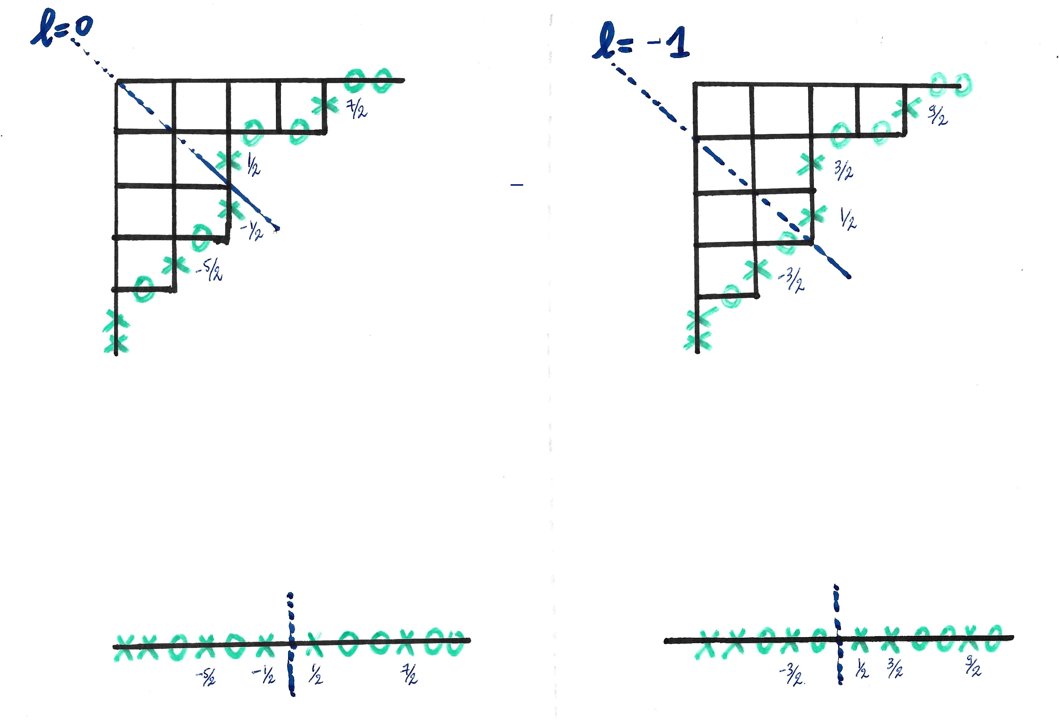
Figure 1: Correspondence between Maya and Young

In this figure, we observe that each pair $(\lambda,l)$ defines the unique Maya diagram, and vice versa. $\Box$ The bosonic space $\mathcal{B}=\mathbb{C}[p_{1},\ldots;z,z^{-1}]=\bigoplus_{l\in\mathbb{Z}}z^{l}\mathbb{C}[p_{1},\ldots]$ is introduced, along with two operators $p_{m}=p_{m}\cdot$ and $p_{-m}=m\frac{\partial}{\partial p_{m}}$ which act on the space $\mathcal{B}$.

The fermionic space $\mathcal{F}:=\bigoplus_{l\in\mathbb{Z}}\mathcal{F}^{l}:=\{v_{i_{1}}v_{i_{2}}\cdots\mid i_{1}>i_{2}>\cdots,i_{k}=-k+l+\frac{1}{2}\text{ for }k\gg 0\}$, in other words, the basis is indexed by Maya diagrams. Is introduced, with two operators $\{\psi_{n},\psi_{n}^{*}\}_{n\in\mathbb{Z}+\frac{1}{2}}$ which act on the fermionic space as follows:

$$\psi_{n}\cdot v_{\lambda}=v_{n}v_{\lambda}$$

$$\psi_{n}^{*}\cdot v_{\lambda}=\begin{cases}0&\text{if }v_{n}\text{ does not appear as a factor in }v_{\lambda},\\ v_{\mu}&\text{if }v_{\lambda}\text{ can be expressed as }v_{n}v_{\mu}\text{ for some }v_{\mu}.\end{cases}$$

Theorem 4 (Boson-Fermion Correspondence).

The bosonic space is isomorphic to the fermionic space, and we have the following correspondences for $m>0$:

$\sum_{i}\psi_{i+m}\psi_{i}^{*}$	$\longleftrightarrow$	$p_{m}$
$\sum_{i}\psi_{i-m}\psi_{i}^{*}$	$\longleftrightarrow$	$p_{-m}=m\frac{\partial}{\partial p_{m}}$
$\sum_{i}:\psi_{i}\psi_{i}^{*}:=\sum_{i<0}\psi_{i}\psi_{i}^{*}-\sum_{i>0}\psi_{i}^{*}\psi_{i}$	$\longleftrightarrow$	$l$

Remark.

We can also consider the mapping:

$$(n,\lambda)\mapsto\prod_{i}p_{\lambda_{i}}|n\rangle$$

where $\ket{n}$ is defined as

$$\ket{n}:=\cdots\times\times\times\times\times\times\bigg{|}_{n}\circ\circ\circ\cdots$$

KP equation from Plucker

We recall that the $\tau$ function in fermionic image can be written as:

(1) $$\tau(t_{1},t_{2},\dots)=\bra{0}g\cdot\exp\left(\sum_{k\geq 1}t_{k}p_{k}\right)\ket{0}=\bra{g}\exp\left(\sum_{k\geq 1}t_{k}p_{k}\right)\ket{0},$$

with $p_{k}=\sum_{j}\psi_{j+k}\psi^{*}_{j}$.

Remark.

the $g$ is a subspace of the space $V$.

Now, let’s construct the KP equation from the Plücker relation.

Let $x=t_{1}$, $y=t_{2}$, $t=t_{3}$, and denote:

$$\langle g|\exp(xp_{1}+yp_{2}+tp_{3})=\langle L^{\prime}|$$

$$v_{-5/2}v_{-7/2}\cdots=|L\rangle$$

$$(a,b,c,d)=(v_{3/2},v_{1/2},v_{-1/2},v_{-3/2})$$

(2) $$\times\times\circ\circ=|0\rangle=v_{-1/2}v_{-3/2}|L\rangle$$

(3) $$\times\circ\times\circ=p_{1}|0\rangle=v_{1/2}v_{-3/2}|L\rangle$$

(4) $$\circ\times\times\circ=\frac{1}{2}(p_{1}^{2}+p_{2})|0\rangle=v_{1/2}v_{-1/2}|L\rangle$$

(5) $$\times\circ\circ\times=\frac{1}{2}(p_{1}^{2}-p_{2})|0\rangle=v_{3/2}v_{-3/2}|L\rangle$$

(6) $$\circ\times\circ\times=\frac{1}{3}(p_{1}^{3}-p_{3})|0\rangle=v_{3/2}v_{-1/2}|L\rangle$$

(7) $$\circ\circ\times\times=\frac{1}{12}(p_{1}^{4}+3p_{2}^{2}-4p_{1}p_{3})|0\rangle=v_{3/2}v_{1/2}|L\rangle.$$

Plücker Relation:

$$\langle L^{\prime}|v_{3/2}v_{1/2}|L\rangle\langle L^{\prime}|v_{-1/2}v_{-3/2}|L\rangle-\langle L^{\prime}|v_{3/2}v_{-1/2}|L\rangle\langle L^{\prime}|v_{1/2}v_{-3/2}|L\rangle+$$

$$+\langle L^{\prime}|v_{3/2}v_{-3/2}|L\rangle\langle L^{\prime}|v_{1/2}v_{-1/2}|L\rangle=0.$$

This can be symbolically written as:

$$\circ\circ\times\times\otimes\times\times\circ\circ-\circ\times\circ\times\otimes\times\circ\times\circ+\circ\times\times\circ\otimes\times\circ\circ\times=0.$$

Substituting 2 – 7 into the Plücker relation:

$$\langle L^{\prime}|\frac{1}{12}(p_{1}^{4}+3p_{2}^{2}-4p_{1}p_{3})|0\rangle\langle L^{\prime}|L\rangle-\langle L^{\prime}|\frac{1}{3}(p_{1}^{3}-p_{3})|0\rangle\langle L^{\prime}|p_{1}|0\rangle|L\rangle+$$

$$+\langle L^{\prime}|\frac{1}{2}(p_{1}^{2}+p_{2})|L\rangle\langle L^{\prime}|\frac{1}{2}(p_{1}^{2}-p_{2})|L\rangle=0.$$

And using that

$$\frac{\partial^{k+l+m}\tau}{\partial x^{k}\partial y^{l}\partial z^{m}}=\langle g|\exp(xp_{1}+yp_{2}+zp_{3})p_{1}^{k}p_{2}^{l}p_{3}^{m}|0\rangle,$$

we obtain:

$$(\tau_{xxxx}+3\tau_{yy}-4\tau_{xt})\tau-4(\tau_{xxx}-\tau_{t})\tau_{x}+3(\tau_{xx}+\tau_{y})(\tau_{xx}-\tau_{y})=0$$

$$\Leftrightarrow\quad (\tau\tau_{xxxx}-4\tau_{xxx}\tau_{x}+3\tau_{xx}^{2})-4(\tau\tau_{xt}-\tau_{x}\tau_{t})+3(\tau\tau_{yy}-\tau_{y}^{2})=0$$

$$\textrm{Soit }\tau=e^{w}$$

$$\Leftrightarrow\quad w_{xxxx}+6w_{xx}^{2}-4w_{xt}+3w_{yy}=0$$

$$\Rightarrow\quad w_{xxxxx}+6w_{xx}w_{xxx}-4w_{xxt}+3w_{yyx}=0$$

$$\Rightarrow\quad \partial_{x}(w_{xxxxx}+6w_{xx}w_{xxx}-4w_{xxt})+3w_{yyxx}=0$$

$$\textrm{Soit }u=w_{xx}$$

$$\Leftrightarrow\quad \partial_{x}(u_{xxx}+6uu_{x}-4u_{t})+3u_{yy}=0$$

Toda lattice

Let’s begin by defining the function $\tau$ similarly:

(8) $$\tau(n,x,y)=\bra{g}\exp(xp_{1,1}+yp_{2,1})\ket{n,-n}$$

where $p_{1,1}=\sum\psi_{1,i+1}\psi^{*}_{1,i}$ and $p_{2,1}=\sum_{i}\psi_{2,i+1}\psi^{*}_{2,i}$.

$$\begin{array}[]{c}\circ\ \circ\\[-3.0pt] \times\ \times\end{array} =\left|\begin{array}[]{c}n-1\\[-3.0pt] -n+1\end{array}\right\rangle,$$

$$\begin{array}[]{c}\times\ \times\\[-3.0pt] \circ\ \circ\end{array} =\left|\begin{array}[]{c}n+1\\[-3.0pt] -n-1\end{array}\right\rangle,$$

$$\begin{array}[]{c}\circ\,\times\\[-3.0pt] \,\times\,\circ\end{array} =p_{1,1}\left|\begin{array}[]{c}n\\[-3.0pt] -n\end{array}\right\rangle,$$

$$\begin{array}[]{c}\times\,\circ\\[-3.0pt] \,\circ\,\times\end{array} =p_{2,1}\left|\begin{array}[]{c}n\\[-3.0pt] -n\end{array}\right\rangle,$$

$$\begin{array}[]{c}\circ\,\times\\[-3.0pt] \,\circ\,\times\end{array} =p_{2,1}p_{1,1}\left|\begin{array}[]{c}n\\[-3.0pt] -n\end{array}\right\rangle,$$

$$\begin{array}[]{c}\times\,\circ\\[-3.0pt] \,\times\,\circ\end{array} =\left|\begin{array}[]{c}n\\[-3.0pt] -n\end{array}\right\rangle.$$

Again, using the same idea from the previous section, the Plücker relation is:

$$\begin{array}[]{c}\times\ \times\\[-3.0pt] \circ\ \circ\end{array}\otimes\begin{array}[]{c}\circ\ \circ\\[-3.0pt] \times\ \times\end{array}-\begin{array}[]{c}\circ\,\times\\[-3.0pt] \,\times\,\circ\end{array}\otimes\begin{array}[]{c}\times\,\circ\\[-3.0pt] \,\circ\,\times\end{array}+\begin{array}[]{c}\times\,\circ\\[-3.0pt] \,\circ\,\times\end{array}\otimes\begin{array}[]{c}\circ\,\times\\[-3.0pt] \,\times\,\circ\end{array}=0.$$

$$\tau(n+1)\tau(n-1)-\tau_{x}(n)\tau_{y}(n)+\tau(n)\tau_{xy}(n)=0,$$

$$\Rightarrow\ \frac{\tau(n+1)\tau(n-1)}{\tau(n)^{2}}=\frac{\tau_{x}(n)\tau_{y}(n)}{\tau(n)^{2}}-\frac{\tau_{xy}(n)}{\tau(n)}=-\frac{\partial^{2}}{\partial x\partial y}\log\tau(n),$$

$$\text{Let }v(n)=\ln\frac{\tau(n+1)\tau(n-1)}{\tau(n)^{2}},$$

$$\Rightarrow\ e^{v(n)}=-\frac{\partial^{2}}{\partial x\partial y}\ln\tau(n),$$

$$\Rightarrow\ 2e^{v(n)}-e^{v(n+1)}-e^{v(n-1)}=\frac{\partial^{2}}{\partial x\partial y}(\ln\tau(n+1)+\ln\tau(n-1)-2\ln\tau(n))=v_{xy}(n),$$

$$\Rightarrow\ v_{xy}=2e^{v(n)}-e^{v(n+1)}-e^{v(n-1)}.$$

Meaning of the Symbol $\ket{n,-n}$

$\ket{2,-2}:=\begin{array}[]{c}\times\ \times\times\ \times\times\ \times\times\ \underset{2}{|}\circ\ \circ\ \circ\\[-3.0pt] \,\times\ \times\times\underset{-2}{|}\circ\ \circ\ \circ\ \circ\ \circ\ \circ\ \circ\end{array}=v_{\frac{3}{2}}v_{\frac{1}{2}}v_{-\frac{1}{2}}v_{-\frac{3}{2}}v_{-\frac{5}{2}}w_{-\frac{5}{2}}v_{-\frac{7}{2}}w_{-\frac{7}{2}}\dots$

Remark.

The Plücker relation remains valid; indeed, $V=V_{1}\oplus V_{2}$ and we still choose $\operatorname{dim}V/L^{\prime}\oplus L=2$, remember that $\mathchoice{{\textstyle\bigwedge}}{{\bigwedge}}{{\textstyle\wedge}}{{\scriptstyle\wedge}}(L_{1}\oplus L_{2})=\mathchoice{{\textstyle\bigwedge}}{{\bigwedge}}{{\textstyle\wedge}}{{\scriptstyle\wedge}}L_{1}\bigotimes\mathchoice{{\textstyle\bigwedge}}{{\bigwedge}}{{\textstyle\wedge}}{{\scriptstyle\wedge}}L_{2}$

The Discrete Function $\tau$

The main idea behind the construction of the discrete function $\tau$ is similar to that of the generalized Toda, except that in this case, we only consider the integers $n_{1},\ldots,n_{s}$. We define the discrete function $\tau$ by:

(9) $$\tau(n_{1},\ldots,n_{s})=\bra{g}\ket{n_{1},\ldots,n_{s}}$$

with $\operatorname{deg}(\textbf{n})=\sum n_{i}=0$.

Theorem 5.

The function $\tau$ satisfies the following octahedral relation for all $\textbf{n}\in\mathbb{Z}^{s}$ such that $\operatorname{deg}(\textbf{n})=-2$, and for any $\alpha<\beta<\gamma<\delta$, we have

(10) $$\tau(\textbf{n}+e^{\alpha}+e^{\beta})\tau(\textbf{n}+e^{\gamma}+e^{\delta})-\tau(\textbf{n}+e^{\alpha}+e^{\gamma})\tau(\textbf{n}+e^{\beta}+e^{\delta})+\tau(\textbf{n}+e^{\alpha}+e^{\delta})\tau(\textbf{n}+e^{\beta}+e^{\gamma})=0$$

where $e^{\alpha}=(0,\ldots,\underset{\text{in the }\alpha\text{-th position}}{1},\ldots,0)$.

Proof.   Note that $\ket{n_{\alpha}+1}=\psi_{\alpha,n_{\alpha}+\frac{1}{2}}\cdot\ket{n_{\alpha}}=v_{\alpha,n_{\alpha}+\frac{1}{2}}\ket{n_{\alpha}}$.

Plücker relation:

$$\bra{g}v_{\alpha,n_{\alpha}+\frac{1}{2}}v_{\beta,n_{\beta}+\frac{1}{2}}\ket{\textbf{n}}\cdot\bra{g}v_{\gamma,n_{\gamma}+\frac{1}{2}}v_{\delta,n_{\delta}+\frac{1}{2}}\ket{\textbf{n}} -$$

$$\bra{g}v_{\alpha,n_{\alpha}+\frac{1}{2}}v_{\gamma,n_{\gamma}+\frac{1}{2}}\ket{\textbf{n}}\cdot\bra{g}v_{\beta,n_{\beta}+\frac{1}{2}}v_{\delta,n_{\delta}+\frac{1}{2}}\ket{\textbf{n}} +$$

$$\bra{g}v_{\alpha,n_{\alpha}+\frac{1}{2}}v_{\delta,n_{\delta}+\frac{1}{2}}\ket{\textbf{n}}\cdot\bra{g}v_{\beta,n_{\beta}+\frac{1}{2}}v_{\gamma,n_{\gamma}+\frac{1}{2}}\ket{\textbf{n}} =0$$

$\Box$

Conjecture 6.

The inverse is also true.

Let $\sigma\in S_{s}$be a permutation. Denote by $\sigma(\textbf{n}):=(\sigma(n_{1}),...,\sigma(n_{s}))$ the action of the permutation on $\mathbb{Z}^{s}$. Define the quadratic form $q_{\sigma}(\mathbf{n})$ as follows:

$$q_{\sigma}(\textbf{n}):=\sum_{\alpha<\beta,\sigma(\alpha)>\sigma(\beta)}i_{\alpha}i_{\beta}$$

Proposition 7.

The permutation group acts on the set of solution octahedral relation 10 by

$$\tau(\textbf{n})\longrightarrow(-1)^{q_{\sigma}(\textbf{n})}\tau(\sigma(\textbf{n})$$

Proof.   It is sufficient to verify that any transposition transforms a solution of 10 to solution of 10. $\Box$

Definition 8.

A function $\tau$ is said to be of double period if there exists a subgroup $G$ of $A_{s-1}=\{\textbf{n}\in\mathbb{Z}^{s}\mid\operatorname{deg}(\textbf{n})=0\}$ of rank 2 such that $\tau$ is invariant under this subgroup. In particular, $\tau$ can be viewed as a function on the quotient $A_{s-1}/G$.

Remark.

By proposition and the definiton of double period of $\tau$ function taht a subgroup can be encoded by convexes polygons with integer vertices.

The double-period function $\tau$ is then defined on the quotient $A_{s-1}/\langle\textbf{a},\textbf{b}\rangle$. In the following examples, we will explore some constructions of integer sequences from the function $\tau$ by taking $s=4$.

Example 9.

The following polygon:

with matrix: $\begin{pmatrix}5&-2&-2&-1\\ 1&1&-1&-1\end{pmatrix}=\begin{pmatrix}\textbf{a}\\ \textbf{b}\end{pmatrix}$. By performing row operations, the matrix becomes $\begin{pmatrix}3&-4&0&1\\ -4&3&1&0\end{pmatrix}$, so the quotient $A_{3}/\langle\textbf{a},\textbf{b}\rangle$ is isomorphic to the group $\{(l,-l,0,0)\mid l\in\mathbb{Z}\}$. Taking $\textbf{n}=(l-1,-l-1,0,0)$, the octahedral relation becomes:

$$\tau(l,-l,0,0)\tau(l-1,-l-1,1,1)-$$

$$\tau(l,-l-1,1,0)\tau(l-1,-l,0,1)+$$

$$\tau(l,-l-1,0,1)\tau(l-1,-l,1,0) =0$$

By the $(\textbf{a},\textbf{b})$-periodicity of the function $\tau$, we deduce:

$$\tau(l,-l,0,0)\tau(-l,-l,0,0)-$$

$$\tau(l+4,-l-4,0,0)\tau(l-4,-l+4,0,0)+$$

$$\tau(l-3,-l+3,0,0)\tau(l+3,-l-3,0,0) =0$$

Letting $a_{l}=\tau(l,-l,0,0)$, the previous octahedral relation becomes:

$$a_{l}^{2}-a_{l+4}a_{l-4}+a_{l-3}a_{l+3}=0$$

$$1,1,1,1,1,1,1,1,2,3,4,5,9,18,34,93,180,348,724,3033,9666,24986,83761,261033,\ldots$$

This is sequence A018896 in OEIS, discovered by Somos [11].

Example 10.

.

The corresponding matrix is $\begin{pmatrix}1&3&-3&-1\\ 0&1&2&-3\end{pmatrix}$. After performing elementary row operations, the matrix becomes $\begin{pmatrix}1&0&-9&8\\ 0&1&2&-3\end{pmatrix}$. Thus, the quotient $A_{3}/\langle\textbf{a},\textbf{b}\rangle$ is isomorphic to the group $\{(0,0,l,-l)\mid l\in\mathbb{Z}\}$. Taking $\textbf{n}=(-1,-1,l,-l)$, the octahedral relation becomes:

$$\tau(0,0,l,-l)\tau(-1,-1,l+1,-l+1)-$$

$$\tau(0,-1,l+1,-l)\tau(-1,0,l,-l+1)+$$

$$\tau(0,-1,l,-l+1)\tau(-1,0,l+1,-l) =0$$

By $(\textbf{a},\textbf{b})$-periodicity of the function $\tau$, we deduce:

$$\tau(0,0,l,-l)\tau(0,0,l-6,-l+6)-$$

$$\tau(0,0,l+3,-l-3)\tau(0,0,l-9,-l+9)+$$

$$\tau(0,0,l+2,-l-2)\tau(0,0,l-8,-l+8) =0$$

Let $a_{l}=\tau(0,0,l,-l)$. The previous recurrence relation becomes:

$$a_{l}a_{l-6}-a_{l+3}a_{l-9}+a_{l+2}a_{l-8}=0$$

$$1,1,1,1,1,1,1,1,1,1,1,1,2,3,4,6,9,13,19,28,41,79,163,490,972,1785,4270,9483,\ldots$$

This sequence is not yet listed in OEIS.

Remark.

To prove that the sequence derived from the octahedral relation is indeed an integer sequence, you can leverage the theory of cluster algebras, particularly using the theorem of Fomin and Zelevinsky.

References

• [1] Peter Tingley, Notes Fock space, 2023, https://arxiv.org/pdf/2211.12463
• [2] Ahmed Lesfari, Courbes algébriques complexe et/ou sufaces de Riemann compactes,2023
• [3] Boris Dubrovin,Integrable Systems and Riemann; https://people.sissa.it/~dubrovin/rsnleq_web.pdf
• [4] Macdonald,Symmetric Functions and Hall Polynomials,Second edition,1995
• [5] He-Chi chan,An invitation to q-series,2011
• [6] M. Sato, Y.Sato, Soliton equations as dynamical systems on infinite dimensional Grass-mann manifolds
• [7] Victor G.Kac, Infinite dimensional Lie algebra,1995
• [8] Serge Lang, Complex Analysis
• [9] Yoko SHIGYO,On Addition Formulae of KP, mKP and BKP Hierarchies,2013, https://arxiv.org/pdf/1212.1952
• [10] L.A.Dickey, Soliton equations and Hamiltonian systems,2003
• [11] M. Sato, M. Noumi, Soliton equations and the universal Grassmann manifold, 1984
• [12] John Harnad and Ferenc Balogh, Tau Functions and their Applications,2021
• [13] Atsushi Nakayashiki, Sigma Function as A Tau Function,2009,https://arxiv.org/pdf/0904.0846v1