Fast ($\sim N$) Diffusion Map Algorithm

Abstract

In this work we explore parsimonious manifold learning techniques, specifically for Diffusion-maps. We demonstrate an algorithm and it’s implementation with computational complexity (in both time and memory) of $\sim N$, with $N$ representing the number-of-samples. These techniques are essential for large-scale unsupervised learning tasks without any prior assumptions, due to sampling theorem limitations.

1 Introduction

One of the major motivations of science, is to collect data and then develop efficient interpretations of this data, effectively compressing it. During a typical experiment modern experimental-apparatuses can capture hundreds of terabytes of weakly-structured digital data. To handle this influx of data, there is an arsenal of compression algorithms. Among the most interoperable are manifold learning (ML) algorithms, and these are well-suited for the unsupervised task of sorting weakly-structured digital data. Our motivation was to consider time-series femtosecond-resolution X-ray-Free-Electron-Laser (XFEL) data. For this, manifold-learning techniques can be used to compress and understand the data. The femtosecond time resolution of the XFEL allows direct access to molecular dynamics of a variety of systems at atomic resolution. Additionally, because XFEL data is natively time-resolved, and methods have been researched to analyze the data to yield Spence, (2014); Fung et al., (2016); Šrajer and Schmidt, (2017). Compact XFELs, currently being developed by Graves et al., (2014, 2017) and Rosenzweig et al., (2020), offer many advantages; however, they produce lower fluence and therefore generate noisier datasets. This introduces unique challenges for the aforementioned ML techniques. Specifically problematic is the $\sim N^{2}$ computational-complexity of existing algorithms. Therefore in this work, we introduce a $\sim N$ scaling algorithm to resolve this issue. This increase in efficiency facilitates the development of real-time, online data analysis and subsequently autonomous-experimentation.

Before we begin, let’s introduce a brief note on the notation used in this paper. In this paper, we index the $N$ samples using Latin characters: $i,j,k$. The $D$-dimensional feature space is indexed by Latin characters: $x,y,z$. Therefore, the dataset is typically represented as a 2-dimensional sample-feature indexed matrix, $R_{ix}$. Convolved dimensions of size $M$ are indexed by uppercase Latin characters: $I,J,K$. Auxiliary indices from reshaping feature dimensions are indexed by $a,b,c$. Before returning to our parsimonious objective, we introduce the relevant manifold learning landscape."

1.1 Diffusion Map

Manifold-Learning is a blend of between regression and compression (i.e. an encoder resulting in an embedding). The central idea of the manifold-technique is that the embedding is strongly continuous. That is, two originally similar high-dimensional samples are encoded by two similar embeddings. There are a variety of manifold-learning algorithms, such as including linear approaches (e.g., Principal Component Analysis (PCA)), and of the nonlinear variety, e.g. Diffusion Maps. The important difference is nonlinear-techniques are able to capture more substantial changes of our samples, e.g. a “manifold” while linear techniques stay within the tangent space of that manifold, see fig.2. We will focus on Diffusion Maps in this work, but much of the ideas introduced here are generalizable to other kernel-based manifold learning techniques (e.g. kernel-PCA). Diffusion Maps, as introduced by Coifman et al., (2005); Coifman and Lafon, (2006), are a highly effective technique to compress a dataset to a low-dimensional nonlinear manifold, and have been thoroughly reviewed by outstanding sources: Rabadán and Blumberg, (2019), Carlsson and Vejdemo-Johansson, (2022), and Dey and Wang, (2022). Here we introduce this technique as a recipe to achieve our objective, and recommend that readers refer to the aforementioned sources for details.

We begin with a dataset as a two-dimensional matrix $R_{ix}$, and compute its pairwise correlation/covariance using a predefined similarity measure, i.e. known as a kernel $k$. The kernel is a well-behaved function $k:\mathbb{R}^{D}\times\mathbb{R}^{D}\rightarrow[0,\infty)$, which takes two samples and yields a scalar measure for their similarity, when applied to all sample-pairs, this yields a covariance-matrix denoted by $k_{ij}$ (a value for sample $i$ compared to sample $j$). The well-behaved nature of the kernel function guarantees the covariance-matrix as Positive-Semi-Definite (PSD). Now we must transform this similarity-matrix into a Markov transition-matrix, this necessitates a couple steps of normalization. The first-step: sum over all rows (xor columns) to obtain a degree vector $D_{i}=\sum_{j}k_{ij}$, then element-wise exponentiate this vector to some power $\alpha$, $D^{-\alpha}_{i}$ (with $i$ as an index, and $\alpha$ as an exponent). To complete the first normalization apply this to both indices of the similarity-matrix $k_{ij}$: $\tilde{k}_{ij}=D^{-\alpha}_{i}k_{ij}D^{-\alpha}_{j}$. The second normalization step, sums the rows to obtain the degree-vector of this matrix: $\tilde{D}_{i}=\sum_{j}\tilde{k}_{ij}$, and applying it (one-sided) to the normalized similarity matrix: $\Delta_{ij}=\tilde{D}_{i}\tilde{k}_{ij}$, the resulting matrix is interpreted as the Graph-Laplacian (a discrete approximation of the Laplace–Beltrami operator), notice that this operator exists on a complete graph (where all nodes are connected, even to themselves), but is weighted. Now that we have constructed our weighted Graph-Laplacian, the dominant eigenvectors specify the embedding.

1.2 Nonlinear Laplacian Spectrum Analysis

Now suppose we wish to compute Diffusion-Maps on time-series data. This is not straightforwardly possible, because repeated motions in the time-series (which are inevitable) would result in closed structures (loops) which lose all time structure. Hence, diffusion-maps can only capture equilibrium behavior. An alternative procedure was introduced by Giannakis and Majda, (2012, 2013); which applied diffusion-map over concatenated-snapshots. Concatenated-snapshots, take $c$ snapshots and form one concatenated snapshot, i.e. $R_{ix}$ now became $R_{IX}$, with $X$ indexing a new feature space over all $c$ snapshots, effectively changing the size from $D$ to $cD$. In practice explicitly constructing $R_{IX}$ requires too much memory; however, the effect of computing it’s diffusion-map kernel was equivalent of taking convolutions with respect to the regular, unconcatenated, snapshot kernel. In particular, with a diagonal convolutional-kernel, i.e. $k_{IJ}=k_{ij}\ast\kappa_{\alpha\beta}$, with $\kappa_{\alpha\beta}\propto\delta_{\alpha\beta}$, the Kronecker-delta. NLSA can be viewed as a generalization of Singular-Spectrum-Analysis (SSA) with Diffusion-Map (DM) replacing the Singular-Value-Decomposition (SVD) step. Note that SSA can itself be viewed as a generalization of Principal-Component-Analysis (PCA), these methods are shown in fig. 1.

Figure 1: The relationship between the 4 mentioned manifold methods.

Figure 2: A depiction of the tangent plane.

2 kernel decomposition

In the spirit of Diffusion-Maps, we desire large-scale structure through diffusion-evolution. With a similar motivation, in 1931 Krylov observed that repeated application of a matrix/operator to an arbitrary initial vector converges to the largest-eigenvector of the system. En-route to this largest-eigenvector, we can obtain a series of vectors that may be orthogonalized to yield the next highest eigenvectors of the matrix. These are precisely the eigenvectors of interest in Diffusion-Map. Lanczos and others later generalized Krylov’s idea into the now-famous iterative Lanczos’ algorithm, which requires only the linear operator function itself rather than the entire explicit matrix. This is the standard method to obtain eigenvectors of very large matrices, and we shall wish to continue with this idea. For Diffusion-Map we have following covariance-matrix we would like to partially-diagonalize:

$$k_{ij} =\exp{\left(-\frac{R^{2}_{ij}}{\sigma^{2}}\right)}\quad.$$ (1)

Unfortunately, the covariance matrix’s memory and computation scales as the square of the number of entries, i.e. $\sim N^{2}$. If we only desire to partially diagonalize; it begs the question why the entire matrix needs to be constructed? Instead if we desire short distance description of the covariance matrix, this may be power-series expanded:

$$k_{ij} =\exp{\left(-\frac{R^{2}_{ij}}{\sigma^{2}}\right)}\quad,$$ (2)

$$=1_{ij}-\frac{R^{2}_{ij}}{\sigma^{2}}+\frac{R^{4}_{ij}}{2\sigma^{4}}+\cdots+\frac{1}{k!}\left(-\frac{R^{2}_{ij}}{\sigma^{2}}\right)^{k}\quad\quad,$$ (3)

$$=\lim_{n\rightarrow\infty}\left(\delta_{ij}-\frac{1}{n}\frac{R^{2}_{ij}}{\sigma^{2}}\right)^{n}\quad\quad,$$ (4)

the truncation of the power-series, eq. 3, is valid for small distances $\sim\frac{R^{2}}{\sigma^{2}}$, which is precisely the motivation of the manifold description. Additionally, at any order the truncation is Positive-Semi-Definite (PSD). Next, we use a commonly used numerical-trick to compute square-distances of the dataset:

$$R^{2}_{i} =\left(\sum_{x}R^{2}_{ix}\right)_{i}$$ (5)

$$\left(R^{2}\right)_{ij} =R^{2}_{i}\otimes 1_{j}+1_{i}\otimes R^{2}_{j}-2\sum_{x}R_{ix}R_{xj}\quad\quad,$$ (6)

unlike eq.2, the equation above is separable. Consequently, this implies at any order eq.3 is also separable. The separability is crucial for avoiding constructing the explicit matrix. Note, although $\delta_{ij}$ is formally of full-rank and not naïvely separable; when matrix-producted with an arbitrary vector, $\sum_{j}\delta_{ij}v_{j}=1_{i}v_{i}$, it is merely the trivial element-wise vector product. We define separable as the ability to compute $\sum_{j}k_{ij}\xi_{j}$ without explicitly constructing the entire $k_{ij}$ matrix, for some arbitrary vector $\xi_{j}$.

3 Feature-Feature Auto-encoder

So far we have only been considering the case of stationary-isotropic kernels, such as the Radial-Basis-Function (RBF) and its relatives. A quick generalization is to consider an anisotropic and non-stationary versions by introducing off-diagonal feature-feature similarities $\delta_{xy}\rightarrow k_{xy}$. Like the ordinary RBF similarity, $k_{xy}$, has hyperparameters that can be tuned or modified. It is now relevant to mention that any PSD-matrix forms a satisfactory kernel-function. Similar to before, this matrix can be abstract only computed as needed or concretely in COOrdinate format (COO) sparse. However, if $k_{xy}$ can be factorized, as we discussed earlier interesting facts emerge. Concretely, let’s consider:

$$k_{xy} =\sum_{\alpha}U_{x\alpha}V^{\dagger}_{\alpha y}\quad\quad.$$ (7)

This Cholesky $U_{x\alpha}$ factor (if $U^{\dagger}=V$), is the embedding matrix, and can embed data not originally apart of our data-set, via the matrix-product $R_{ix}U_{x\alpha}$. Thus, this is clearly an important component to possess, especially for online learning. Auto-encoder theory has been well-developed, e.g. refer to Bengio et al., (2017), and combined with the explosive field of neural-networks, and these could lead to interesting kernels, whilst being separable for efficient computation as suggested by this work.

Figure 3: Auto-encoder.

3.1 Graphs

In the spirit of diffusion-maps, we may take the auto-encoder to be the graph-Laplacian, i.e. $k_{xy}=\Delta^{(G)}_{xy}$, with nodes of this graph representing each feature (or pixel, in our context). This defines a pullback-like operation, akin to differential-geometry, whereby we have a connection between the feature and sample “manifolds” or rather the discrete graphs/networks. The first approach might involve a random grap, however in our circular-toy model this introduced strong anisotropies, therefore a random regular graph might be the best choice (treating all pixels equally, where all nodes have the same degree, or number of connections).

2D Lattice Graph Laplacian

Because, in our context, the nodes are pixels, and pixels are commonly in 2d-arrays, the most straightforward approach to model this function would be to use nearest neighbors. The adjacency-matrix for the 2d-periodic (toroidal) lattice can be reshaped (denoted by $\rightarrow$) and factored as:

$$A_{xy}\rightarrow A_{abcd} =\delta_{ac}\otimes M_{bd}+M_{ac}\otimes\delta_{bd}\quad\quad.$$

Then if we have a feature vector, it may be reshaped to a matrix $R_{x}\rightarrow R_{ab}$. Then

$$A_{xy}R_{y} =v_{x}=v_{ab}=\sum_{c}R_{ac}M_{cb}+\sum_{c}M_{ac}R_{cb}\rightarrow R_{x}\quad\quad,$$

$M$ is the cycle graph adjacency-matrix. This idea of using graphs that are a result of tensor-products (e.g., higher-dimensional lattices like 4D lattices) is easily generalizable. That is, if the feature-feature connectivity Graph can be decomposed as $G=G_{1}\times G_{2}\times\cdots\times G_{d}$, then the associated adjacency-matrix is the tensor-product of the corresponding adjacency-matrices: $A=A_{1}\otimes A_{2}\otimes\cdots\otimes A_{d}$, with $G_{d}\sim A_{d}$. If we choose $G_{i}$’s to be the cycle-graph $C_{n}$, then the total graph $G$ has well-behaved features: regular and fully connected (i.e., not disjoint). Furthermore, applying the contracted vector to this feature-Laplacian can be done more efficiently in sequence, achieving a complexity of $\sim dDD^{1/d}$. All these techniques are separable in the sense as described earlier. Additionally, even if the graph is not tensor-decomposable (or similar), sparse-matrix representation is likely very adequate for the graph-Laplacian. Hence both the tensor-decomposition or the sparse matrix-product may be efficient to compute $\Delta_{xy}\tilde{R}_{y}$. This should not be done in dense-format in order to avoid the $\sim D^{2}$ computational-complexity, as for large feature dimensions $N\approx D$, this voids the desired gains.

4 The Linear Operator

Now that we have motivated the pieces let’s put them together. However, we are still missing one element, if we wish to implement NLSA, we require the convolution of the diffusion map’s kernel/covariance-matrix. This cannot be done explicitly, as this would once again void the $\sim N$ scaling. Instead, it turns out we can decompose the convolution on-the-fly as well. The key is to have a formula for the kernel that we wish to convolve, that is already factored, e.g.:

$$k_{ij}\propto R_{ix}R^{\dagger}_{xj}\quad\quad.$$

Next, the convolution requires certain pieces of $R^{\dagger}$ to mix with certain pieces of $R$, note the internal index $x$ is irrelevant for this operation. These certain pieces are the entries we need to sum over, these specific pieces are by a series of indices: $I_{\beta},J_{\beta}$, which compose $R,R^{\dagger}$ before computing the inner-product over $x$. This is achieved as follows:

$$k_{ij}\ast\kappa_{\alpha\beta} =\left(\sum_{\alpha\beta}\,\kappa_{\alpha\beta}\sum^{D}_{x,y}R_{ix}[I_{\beta},:]k_{xy}R^{\dagger}_{yj}[:,J_{\beta}]\right)_{IJ}\quad\quad.$$ (8)

This algorithm scales as $\sim c$ (number of convolutional-kernel entries); however, further improvements may be possible for very high convolutions. When combined with the other components we may now construct our linear operator, starting with one-step of eq. 4 (without the $R^{2}\oplus R^{2}$ term),

LO $$=\left(\delta_{IJ}+2\sum^{c}_{\alpha\beta}\kappa_{\alpha\beta}\sum^{D}_{x,y}R_{ix}[I_{\alpha},:]k_{xy}R_{yj}[:,J_{\beta}]\right)\quad\quad.$$ (9)

This linear operator takes a vector as input and returns another, effectively applying the following operation: $\text{LO}\xi_{j}=\xi_{i}=k_{ij}\xi_{j}$. Notice that the summation is performed as soon as this vector is made concrete. To address the question of normalization, we apply the linear operator to the ones-vector (a 1D array consisting of all ones). This yields the row (or column, as this LO is symmetric) sum, which may be altered à la diffusion-map by the aforementioned $\alpha$ exponent. This result $D_{I}$, may be used to create a new operator:

$$D_{I} =\left(\quad(\text{LO}\left(1_{J}\right))^{(-\alpha)}\quad\right)\quad\quad,$$

$$\tilde{\text{LO}} =D_{I}\left(\delta_{IJ}+2\sum^{c}_{\alpha\beta}\kappa_{\alpha\beta}\sum^{D}_{x,y}R_{ix}[I_{\alpha},:]k_{xy}R^{\dagger}_{yj}[:,J_{\beta}]\right)D_{J}\quad\quad.$$

Applying this operator to a vector of size $M$, has computational complexity of $\sim cMD$, where $c$ is the convolutional size, $M$ is the final-convolved-sample size, and $D$ feature size.

5 Results

In order to test the scaling of our algorithm, we introduce the following test. We consider an ensemble of $N$ randomly rotated images, as shown in fig. 4, to form a dataset $R_{ix}$. We know a priori that the desired manifold is a circle or rather the parametric 2-dimensional circle, therefore we require the three largest eigenvectors and eigenvalues of the Laplacian-operator for our diffusion-map analysis. These are incorporated into our algorithm, and we track the execution times for our implementation on an NVIDIA H100 GPU. The results for one simulation are plotted in fig. 5, and the timings for our dataset are displayed on fig. 6. The timing results, fig. 6, show a clearly linear scaling with $N$ substantiating our claim.

Figure 4: $127\times 127$ pixel icon used to calibrate the diffusion-map algorithm.

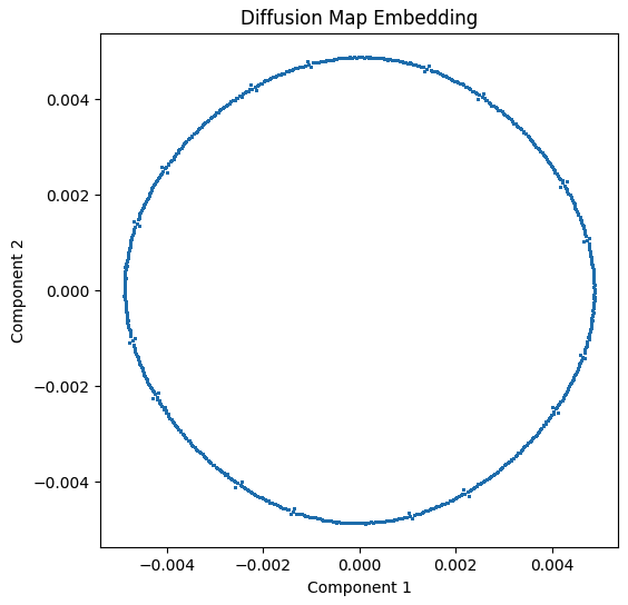
Figure 5: Example of a Diffusion Map embedding result for $\sim 50,000$ snapshots, with the aforementioned fig. 4.

Figure 6: This plot demonstrates the linear $\sim N$ scaling of the algorithm. Although it appears exponential, this is because of the scale of the $x$-axis. The approximate fit has a linear equation: $t=6\times 10^{-6}\times N+0.65$ seconds.

6 Conclusions

The central idea of this work was to compute the eigenvectors and eigenvalues directly without explicitly constructing the $\sim N^{2}$ kernel, this approach has the benefit of computing an exact spectrum. However, other approaches could have also been used to obtain $\sim N\log N$ scaling approximately, namely using graph-partitioning, based on the work of Karypis and Kumar, (1998), which scales pseudolinearly to pre-filter the dataset into similar batches. Ultimately, an approach like this might have to be used once the RAM memory is exhausted at $\sim ND$. This is now the primary limitation for this algorithm and any realistic implementation. Interestingly, in our effort to find a factorization of the kernel-matrix, we realized that the anisotropic kernel could be interpreted as an auto-encoder. Parts of the auto-encoder could be useful for compressing the data-set, in order to exceed the aforementioned memory limitations, or more intriguingly, to implement online compression to facilitate reinforcement-learning or Gaussian-process, Noack et al., (2023), based autonomous-experimentation.

Appendix A Background Code

A.1 Lanczos Solver

⬇

import jax

jax.config.update("jax_enable_x64", True)

import jax.numpy as jnp

from functools import partial

@partial(jax. jit, static_argnums=(0,1))

def jeigsh(LO, k=6, =1.E-14, Largest=True, key=jax.random.PRNGKey(0), DTYPE=jnp.float64):

N=LO.shape[0] ## matrix-size

m = int((N)**(k/N)) + (1-k//N)*k*(N.bit_length()-1)

#c = jax.lax.select(Largest, -1., 1.)

##########################################

@jax. jit

def Gram_Schmidt_(i, Data):

V_, K = Data

v = K[i, :]

V_ -= (jnp.conj(v) @ V_) * v

return [ V_, K ]

@jax. jit

def Lanczos_( Data ):

#### inputs

V_, K, , , _, , i = Data

#### compute

V_ = V_.reshape(-1)

_ = jnp.sqrt( V_ @ V_ )

V_ /= _

### GRAM-SCHMIDT

V_, K = jax.lax.fori_loop(0, i, Gram_Schmidt_, [V_, K])

AV = LO(V_)

#AV *= c

AV = AV.reshape(-1)

_ = jnp.conj(V_) @ AV

AV -= V_ * _

AV -= K[i-1,:] * _

K = K.at[ i,: ]. set(V_)

= .at[ i-1 ]. set(_)

= .at[ i-1 ]. set(_)

return [ AV, K, , , _, , i+1 ]

@jax. jit

def if_( Data ):

"""

i (iteration)

max_i (maxiteration)

"""

_, K, _, _, _, , i = Data

def check_(check_values):

_, = check_values

return jax.lax.cond(_ < , False, lambda x:x, True, lambda x:x)

return jax.lax.cond(i < K.shape[0], [_, ], check_, False, lambda x:x)

##########################################

#### initialize data required for calculation

v_0 = jax.random.uniform(key, (N,), dtype=DTYPE) ## initial guess eigenvector

kV = jnp.zeros((m+1, N), dtype=DTYPE) ## Krylov Vectors

= jnp.zeros(m, dtype=DTYPE) ## diag of Lanczos Matrix

= jnp.zeros(m, dtype=DTYPE) ## off-diag of Lanczos Matrix

Data = [v_0, kV, , , 1.0, , 1]

v_f, kV, , , _, _, iter = jax.lax.while_loop( if_, Lanczos_, Data)

kV = kV.at[ iter,:]. set(v_f)

kV = kV[1:,:]

#### Oh use LinearOperator for Tridaigonal??? restarted Lanczos!

A_tridiag = jnp.diag()

A_tridiag += jnp.diag( [1:], 1)

A_tridiag += jnp.diag(jnp.conj([1:]), -1)

#### get eigen-values/vectors & Unitary matrix (m x m) matrix, N -> m -> k?

eigvals, U = jnp.linalg.eigh(A_tridiag) ## ~m^3, only need k

eigvals = eigvals.astype(A_tridiag.dtype)

#eigvals *= c

#### get eigenvectors

#eigvecs = (U.T[:k,:] @ kV)

eigvecs = (U.T[-k:,:] @ kV)

#return eigvals[:k], eigvecs

return (eigvals[-k:]), eigvecs.T

References

- Bengio et al., (2017) Bengio, Y., Goodfellow, I., and Courville, A. (2017). Deep Learning, volume 1. MIT press Cambridge, MA, USA.
- Carlsson and Vejdemo-Johansson, (2022) Carlsson, G. and Vejdemo-Johansson, M. (2022). Topological Data Analysis with Applications. Cambridge University Press.
- Coifman and Lafon, (2006) Coifman, R. R. and Lafon, S. (2006). Applied and Computational Harmonic Analysis, 21(1):5–30.
- Coifman et al., (2005) Coifman, R. R., Lafon, S., Lee, A. B., Maggioni, M., Nadler, B., Warner, F., and Zucker, S. W. (2005). PNAS, 102(21):7426–7431.
- Dey and Wang, (2022) Dey, T. K. and Wang, Y. (2022). Computational Topology for Data Analysis. Cambridge University Press.
- Fung et al., (2016) Fung, R., Hanna, A. M., Vendrell, O., Ramakrishna, S., Seideman, T., Santra, R., and Ourmazd, A. (2016). Nature, 532(7600):471–475.
- Giannakis and Majda, (2012) Giannakis, D. and Majda, A. J. (2012). PNAS, 109(7):2222–2227.
- Giannakis and Majda, (2013) Giannakis, D. and Majda, A. J. (2013). Stat. Anal. Data Min., 6(3):180–194.
- Graves et al., (2014) Graves, W., Bessuille, J., Brown, P., Carbajo, S., Dolgashev, V., Hong, K.-H., Ihloff, E., Khaykovich, B., Lin, H., Murari, K., et al. (2014). Physical Review Accelerators and Beams, 17(12):120701.
- Graves et al., (2017) Graves, W., Chen, J., Fromme, P., Holl, M., Kirian, R., Malin, L., Schmidt, K., Spence, J., Underhill, M., Weierstall, U., et al. (2017). Asu compact xfel. In Proc. 38th International Free-Electron Laser Conference (FEL’17).
- Karypis and Kumar, (1998) Karypis, G. and Kumar, V. (1998). SIAM Journal on Scientific Computing, 20(1):359–392.
- Noack et al., (2023) Noack, M. M., Krishnan, H., Risser, M. D., and Reyes, K. G. (2023). Sci. Rep., 13(1):3155. arXiv:2205.09070.
- Rabadán and Blumberg, (2019) Rabadán, R. and Blumberg, A. J. (2019). Topological Data Analysis for Genomics and Evolution: Topology in Biology. Cambridge University Press.
- Rosenzweig et al., (2020) Rosenzweig, J., Majernik, N., Robles, R., Andonian, G., Camacho, O., Fukasawa, A., Kogar, A., Lawler, G., Miao, J., Musumeci, P., et al. (2020). New Journal of Physics, 22(9):093067.
- Spence, (2014) Spence, J. (2014). Faraday Discussions, 171:429–438.
- Šrajer and Schmidt, (2017) Šrajer, V. and Schmidt, M. (2017). Journal of Physics D: Applied Physics, 50(37):373001.