Using lateral dispersion to optimise microfluidic trap array efficiency

Abstract

Microfluidic Trap Arrays (MTAs) have proved to be efficient tools for several applications requiring working at the single cell level like cancer treatment or immune synapse research. Even though several hydrodynamic trapping devices have been already optimised, Two-Dimensionnal (2D) single layer MTAs offering a high trap density remain partially efficient. Indeed, it generally appears that many traps stay empty, even after a long time of injection which can drastically reduce the number of samples available for post-treatment. It has been shown that these unfilled traps are due to the symmetrical nature of the flow around the traps, and breaks in symmetry improve capture efficiency. In this work, we use a numerical approach to show that it is possible to generate optimal geometries that significantly improve filling efficiency. This efficiency is associated with an increase in the lateral dispersion of the objects. Then, we show that adding disorder to the layout of the traps is the most interesting solution and may stay efficient independently of the trap array size.

Keywords

Microfluidics, trapping, optimisation, CFD

1 Introduction

Among the last discoveries in medicine and biology research, Microfluidic Trap Arrays (MTAs) appear as very promising tools for several applications like research concerning tumorous cells response to drugs [1, 2], leukemia cells identification [3], stem cells aggregate analysis [4] or immune response triggering [5, 6]. This success is due to the fact that MTAs allow an accurate spatio-temporal control of numerous and various isolated micro-sized objects such as cells [7, 5, 8, 9, 10], droplets [11, 12, 13, 14, 5, 15], or beads [16, 14, 10]. Hydrodynamic MTAs (HMTAs) working principle is the following: objects are diluted inside a fluid, flowing through a microfluidic chamber constituted by an array of a large number of traps. While following the fluid flow by viscous drag, objects can be caught in the traps individually or by small groups. Trapping can be achieved passively by gravity [17, 15, 18, 19], inertial lift [19], permanent magnets [20, 21] or actively using valves [22, 23], optical tweezers [24], dielectrophoresis [25, 10], electromagnets [26] and acoustics [27]. However, these techniques are contingent on the physical properties of the objects, frequently necessitating more intricate designs, materials, manufacturing processes, and incurring higher costs, thereby constraining their integration into regular clinical practice. On the contrary, HMTAs mechanism relies only on the carrier fluid properties and objects geometry. HMTAs offering the highest trap surface density are two-dimensional (2D) with traps regularly disposed in a staggered pattern inside a Hele-Shaw cell [8, 5, 6, 9, 7]. Even though several hydrodynamic trapping devices have been already optimised, Two-Dimensionnal (2D) single layer MTAs remain partially efficient. Indeed, it generally appears that many traps stay empty, even after a long time of injection which can drastically reduce the number of samples available for post-treatment [9]. The trapping efficiency of these devices can be enhanced using double layered lithography techniques [7, 8, 5] but it complicates their fabrication process. In order to improve capture performance of single layer 2D HMTAs, a numerical approach seems perfectly appropriate for exploring different experimental configurations (geometry, flow properties, density of objects to be captured, etc…) To this end, we can cite [28, 29, 30, 31, 32, 33, 19] who improved the trap and channels geometry or [34, 16] who enhanced the trap relative positions and orientations with respect to the main flow for different hydrodynamic trapping devices. However, all these numerical studies focused on devices with a few number of traps. Recently, we experimentally validated a Computational Fluid Dynamics (CFD) and particle tracing approach in a 2D rectangular HMTA of $100$ traps [14]. Interestingly, we proved the importance of the flow structure in the chamber and of breaking symmetries along the cavity to enhance the capture efficiency by favouring lateral dispersion. In this work, we propose to go a deep further by adapting our CFD/particle model to a fully parameterised geometry and to couple it with optimisation algorithms to maximise the MTA’s trapping efficiency. In a first approach, the trapping efficiency is optimised independently on five dimensionless geometric parameters. In a second set of numerical experiments, we show that similar trapping efficiencies can be reached using disordered trap arrays. The physical interpretation we propose is based on considering the flow structure along the cavity. Then we provide a preliminary experimental study on one example of disordered MTA geometry and we find the expected filling efficiency. We believe this new geometry opens new routes for very large scale trapping of biological objects and could contribute to the generation of patient specific biological big data at the single cell scale.

2 Materials and methods

The whole numerical model is developed using the commercial Finite-Element software COMSOL Multiphysics ® while post-processing is achieved with Python.

2.1 parameterised geometry

We study a single layer MTA of $98$ traps as previously [14]. Because of symmetry, a $2$D model built from parameterised geometric primitives is suggested (Figure 1). The MTA is initially organised in a rectangular staggered pattern of axis $(Ox)$ in the streamwise direction and of axis $(Oy)$ in the lateral direction, (see Figure 1 where all the geometrical parameters are sketched). The dimensions of the MTA are $l$ and $w$ and the one of the cavity are $L$ and $W$ in the streamwise resp lateral directions ; and the distances between the traps are respectively $\Delta x$ and $\Delta y$. We call "chamber" the whole system including the MTA and the cavity. For more information, all the fixed geometric parameters of the model are reported in supplementary Table S1 section S1.1.

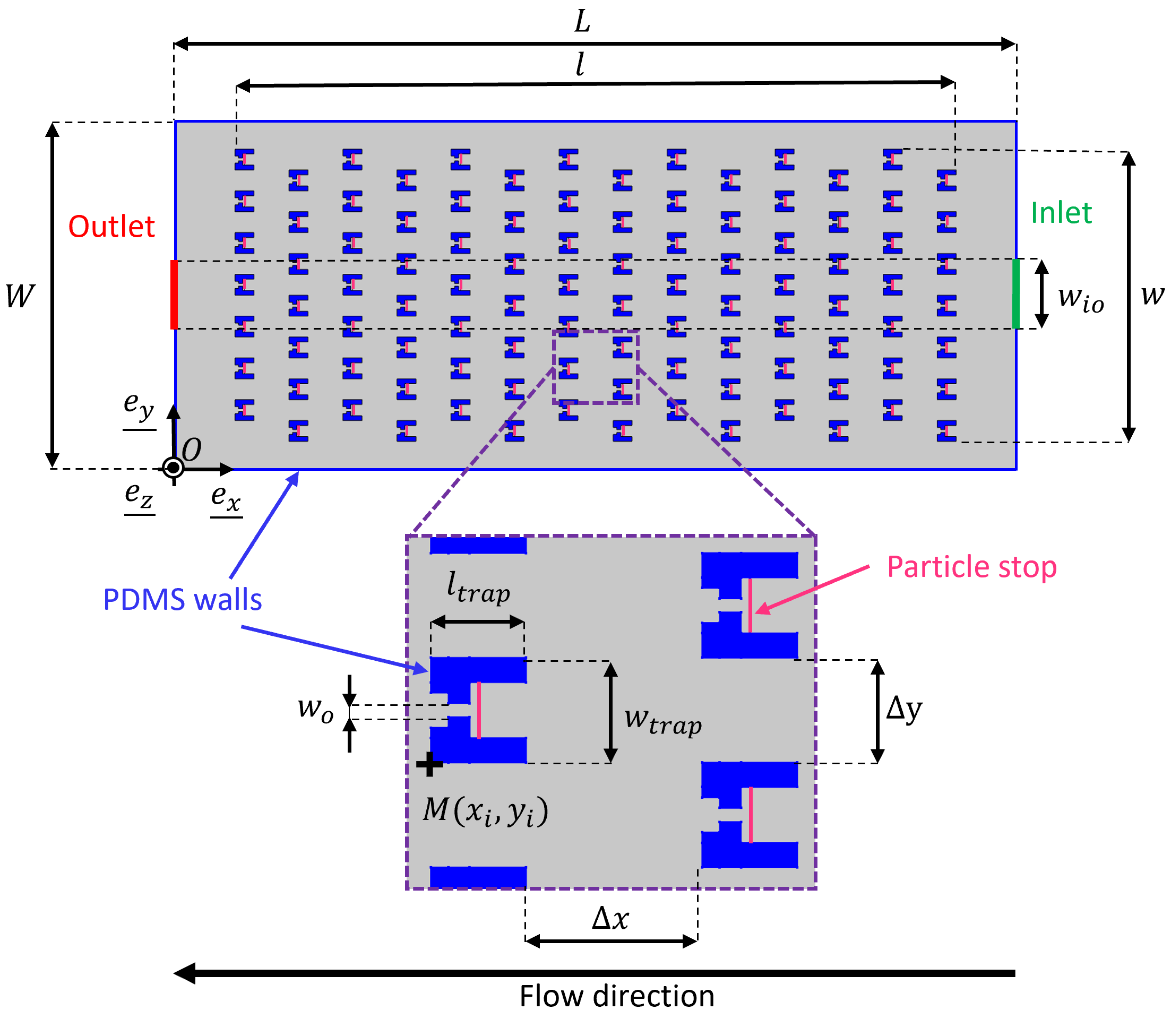
Figure 1: The model geometry. The fluid domain is represented in grey, the traps and the PDMS walls in blue, the inlet resp outlet channels in green resp in red. A particle stop frontier is added in each trap (in pink) to virtually stop particles without modifying the fluid flow.

2.2 Physics of the problem

We consider the flow as incompressible, stationary and the fluid as Newtonian. Furthermore, the maximal Reynolds number $Re=\frac{Uh}{\nu}$ (where $U\sim 1$ mm s^-1 is the maximal mean velocity, $h=14$ µm the height of the cavity and $\nu=10^{-6}$ m² s^-1 the kinematic viscosity of the solution) is about $Re=0.01$, which allow us to consider the Stokes equations. In order to simplify the study, the fluid flow is reduced in 2D in the in-plan of the cavity (ie $(O,\underline{e_{x}},\underline{e_{y}})$, Figure 1) and verifies the Brinkman equations that account for both viscous dissipation in the in-plane and in the out-of-plane direction of the cavity (ie $(O,\underline{e_{z}})$, Figure 1) through a force $\underline{f}$. As such, the latter equations read:

$$\begin{cases}-\nabla p+\mu\nabla^{2}\underline{v}+\underline{f}=\underline{0}\\ \nabla.\underline{v}=0\end{cases}$$ (1)

where $p$ is the pressure field, $\mu$ the fluid dynamic viscosity, $\underline{v}$ the velocity field. The chamber is horizontally orientated such that gravity does not contribute to the flow. The friction force $\underline{f}$ is given in the shallow channel approximation by:

$$\underline{f}=-\frac{12\ \mu}{h^{2}}\ \underline{v}$$ (2)

Therefore, $\underline{v}$ corresponds to the depth-averaged velocity field in-plane (in 2D). As boundary conditions, uniform pressures are applied on the inlet $p_{in}=100$ Pa and outlet $p_{out}=0$ Pa boundaries. On the PDMS walls, the viscous fluid-solid interaction forces a zero fluid velocity $\underline{v}=\underline{0}$. First, equations 1, 2 and the latter boundary conditions are numerically solved to calculate the stationary flow $\underline{v}$. To do so, these equations are translated into a mixed weak formulation and are discretised in space by applying the Finite-Element Method (FEM) with linear Lagrange interpolation functions for both pressure and velocity fields. For more information see supplementary section S1.2.
We study a dispersion of polystyrene (PS) particles of diameter $D_{p}=5$ µm and of concentration $C_{p}=10^{6}$ mL^-1. This concentration is sufficiently small that particles do not modify the viscosity of the suspending fluid and leads to a typical distance between particles about $62$ µm which allows neglecting particle interactions. Furthermore, the particles diffusion coefficient is about $8.7\ 10$^-14 m² s^-1 which makes particle diffusion negligible with respect to particle convection. Despite a low Reynolds number, the Lifto-Diffusif number is ${\cal N}=\frac{27\pi V^{2}\rho R_{p}^{4}}{2k_{b}Th}\sim 30$, thus, lift forces are non-negligible in our flow conditions [35]. However, the corresponding maximal depletion thickness at the outlet of the chamber is $\delta=\sqrt{\frac{R_{p}\rho L}{Wh^{2}\mu}}\sim 1.3$ µm which is small compared the particle size of $5$ µm, such deviations will thus be disregarded in the following. The PS particles density of $1.05$ g ml^-1 is very close to the carrier fluid one, thus particle sedimentation will be also disregarded. As the Reynolds number is low and that the particles are three times smaller than the channel height, we make the assumption that the particle center of mass trajectories are similar to the carrier fluid streamlines (neglected size). Their equation of motion is obtained considering a purely advective transport:

$$\frac{\partial\underline{r}}{\partial t}=\underline{v}$$ (3)

where $\underline{r}$ is the particle position. When a particle enters into a trap, it is artificially stopped at a stop boundary in each trap (pink boundaries Figure 1). Experimentally, it is impossible to perfectly control the particle initial positions at the inlet. Therefore, we try to sweep the most possible every positions on the inlet by regularly placing $N_{p}=200\ (\approx 2\times\,\rm{number\ of\ traps}$) particles on the inlet boundary. Equation 3 is discretised in time and integrated using an implicit generalised-alpha numerical scheme.

2.3 Geometry parametric analysis

From a purely applications perspective, the reader can refer to sections 3.2 outlining the optimum characteristics of a high-performance MTA. This section presents the definition of the different parameters that are used for the optimisation of the MTA. We first have to define the objective of the optimisation. As several particles can be captured in a same trap, we make a distinction between the filling efficiency $E_{fill}$ i.e. the proportion of occupied traps by at least one particle:

$$E_{fill}=\dfrac{number\ of\ occupied\ traps}{number\ of\ traps}$$ (4)

and the capture efficiency $E_{capt}$ i.e. the proportion of trapped particles:

$$E_{capt}=\dfrac{number\ of\ trapped\ particles}{number\ of\ particles}$$ (5)

Since the number of particles ($\sim 2\ number\ of\ traps$) is greater than the number of traps, we can expect that $E_{fill}>E_{capt}$. In order to optimise these objectives, several dimensionless geometric parameters, defined arbitrarily by us, have been varied:

• The centering $C$ represents the shift between the inlet and outlet channels in the lateral direction and thus allows studying symmetry/asymmetry effects between the inlet and the outlet. Its value is $100\%$ when the inlet and the outlet are perfectly aligned (as in Figure 1) and $0\%$ when the shift is maximal. $C$ is given by:

  $$C=1-\frac{\Delta y_{io}}{\Delta y_{io\ max}}=1-\frac{2\ \Delta y_{io}}{W-w_{io}}$$ (6)

  where $\Delta y_{io}$ is the lateral distance between the inlet and outlet and $\Delta y_{io\ max}$ is its maximal value.

• The width ratio $W_{r}$ in the lateral direction between the trap array and the cavity width is defined by:

  $$W_{r}=\frac{w}{W}$$ (7)

  This ratio allows to investigate the role of a particle bypass on the sides of the cavity.

• The length ratio $L_{r}$ in the stream direction between the trap array and the cavity length is defined by:

  $$L_{r}=\frac{l}{L}$$ (8)

  This ratio allows investigating possible entrance effect of particle distribution.

• The trap array aspect ratio $A_{r}$ is defined by the ratio between the number of lines $N_{l}$ in stream direction and the number of columns $N_{c}$ in lateral direction of the trap array:

  $$A_{r}=\frac{N_{l}}{N_{c}}$$ (9)

  This ratio is maybe the less intuitive, but we will see that it may play a role. Most studies show MTA with an $A_{r}<1$ but without motivating this choice. We thus intend to inspect its role.

• And finally, in order to characterize the importance of the channel width occupied by particles at the inlet, we introduce, the inlet and outlet channels to cavity width ratio in the lateral direction:

  $$Wch_{r}=\frac{w_{io}}{W}$$ (10)

All the MTAs described in the literature have a regular trap distribution in the cavity. We therefore question the role of this regularity and how the results are affected when disorder is introduced into the traps positioning. To do so, we start from a regular trap position structure (Figure 1) and introduce irregularities in the trap network. This is achieved by applying a randomized translation along the horizontal and vertical directions of each trap "$i$":

$$\begin{cases}x_{i}=x_{oi}+\psi_{x}(i)\ D_{f}\ \Delta x\\ y_{i}=y_{oi}+\psi_{y}(i)\ D_{f}\ \Delta y\\ \end{cases}$$ (11)

where $(x_{i},y_{i})$ are the coordinates of the $i^{th}$ trap bottom left corner (point $M$ in Figure 1), $(x_{0i},y_{0i})$ its original coordinates following the rectangular staggered pattern, $\psi_{x}$ and $\psi_{y}$ are independent random distributions of numbers between $-1$ and $1$, $D_{f}$ a positive constant called "disorder factor" between $0$ and $1$. We have tested two ways of introducing disorder into the lattice, uniform and centered Gaussian with a standard deviation of $0.3$ distributions for $\psi_{x}$ and $\psi_{y}$.

2.4 Preliminary experimental protocol

The precise microfabrication steps are the same as those for [14] and are very briefly mentioned in this section. A microfluidic chamber resulting from disorder study is fabricated using single layer standard photo-lithography techniques. Basing on previous MTA studies in the literature, we have chosen to connect $4$ MTAs in parallel [8] (Figure 2b). A chrome photomask is fabricated from the geometry files of the simulations by direct laser writing. A circular $h=14$ µm thick layer of photoresist resin is generated on a silicon wafer following a spin coating protocol. A master is obtained by UV-light activation and dissolution of the non-activated photoresist resin. PDMS is mold on the master and the microfluidic chip is closed by sticking a glass coverslip on the chip following a plasma activation protocol. The microfluidic chip is then observed using fluorescent microscopy with a 10X magnification (Figure 2a). The inlet and outlet channels are connected to a pressure controler with a pressure drop $\Delta p$ corresponding to a flow rate $Q_{v}=0.5$ µl min^-1 and a $C_{p}=10^{6}$ ml^-1 concentrated solution of fluorescent particles, hydraulic resistance variation of the chip is negligible during all the experiment [14].

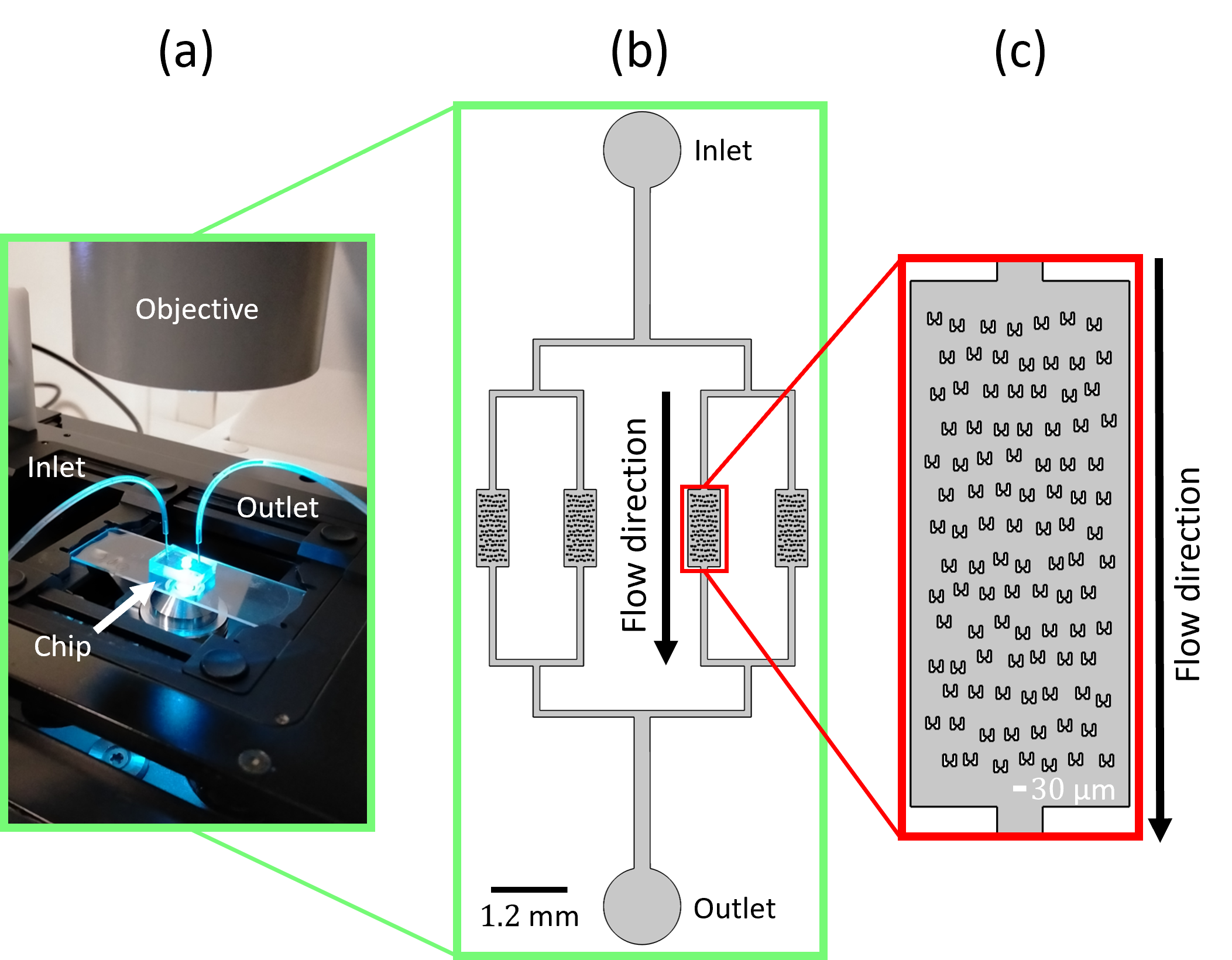
Figure 2: Experimental setup. (a) The microfluidic chip containing the channels is placed on the microscope plate, its inlet and outlet are connected via tubes to a pressure regulator. (b) Scheme of the $4$ microfluidic chambers linked to the inlet and outlet where the tubes are anchored. (c) One of the 4 fabricated chambers observed with a binocular magnifier.

3 Results and discussion

3.1 Parametric study of cavity geometry

We study the influence of the $5$ cavity dimensionless parameters: $C$, $W_{r}$, $L_{r}$, $A_{r}$ and $Wch_{r}$ on filling $E_{fill}$ and capture $E_{capt}$ efficiencies defined in the section 2.3. Each parameter’s influence is screened over 10 values while keeping the other parameters constant. We see on the Figure 3a that filling and capture efficiencies are $96\%$ correlated over the $50$ corresponding simulations. Therefore, optimising the MTA geometry with $E_{fill}$ or $E_{capt}$ as objective function should give similar trends and optimum parameter values. Then, we focus the study on filling efficiency only. The results in capture efficiency are provided in supplementary Figure S1 section S2.1.

Figure 3: (a) Filling efficiency as a function of capture efficiency for each parametric study, the linear correlation coefficient is $\rho_{corr}=96\%$. (b) Influence of the five cavity dimensionless parameters $C$, $W_{r}$, $L_{r}$, $A_{r}$ and $Wch_{r}$ on filling efficiency. When parameters are fixed, their respective values are: $C=100\%$, $W_{r}=84\%$, $L_{r}=86\%$, $A_{r}=0.50$ and $Wch_{r}=23\%$ which corresponds to the reference geometry Figure 1. For each study, the best geometry is obtained for: $C=55.5\%$, $W_{r}=64\%$, $L_{r}=90\%$, $A_{r}=1$ and $Wch_{r}=10\%$. Results from a same parametric study are connected by dashed lines to improve readability.

Figure 3b summarises the evolution of filling efficiency for a regular MTA. It is clear that all the cavity parameters have an influence on $E_{fill}$ between $\pm 20\%$ for the $W_{r}$ parameter (red triangles) and $\pm 44\%$ for the $A_{r}$ parameter (khaki stars). The maximal (resp minimal) filling efficiency is obtained for an inlet/outlet centering $C=55.5\%$ (orange big circle) and $19\%$ for an aspect ratio $A_{r}=3.8$. The corresponding maximal and minimal filling efficiencies are respectively $77\%$ and $19\%$. Setting properly these parameters is therefore crucial for a good chamber design. It is difficult to extract clear trends in filling efficiency as a function of the various parameters because most of these are non-monotonic. However, we notice that small inlet/outlet channels (low $Wch_{r}$) are more efficient than wide ones (high $Wch_{r}$) and the proximity of inlet/outlet channels to the trap array (high $L_{r}$) also enhances filling efficiency.

Figure 4a shows the particle trajectories and final positions in the best geometry we get so far (corresponding to the big orange point previous Figure 3b). We see that trapped particle trajectories exhibit zigzag-like patterns between traps that are slightly deflected in the lateral direction (from the left to the right, red trajectories Figure 4a). We previously highlighted the performances of such oblique flow in the case of a maximal inlet/outlet shift ($C=0\%$) [14], but it seems that an optimum inlet/outlet shift exists for a relative centering $C$ between $44\%$ and $66\%$ (Figure 3b).

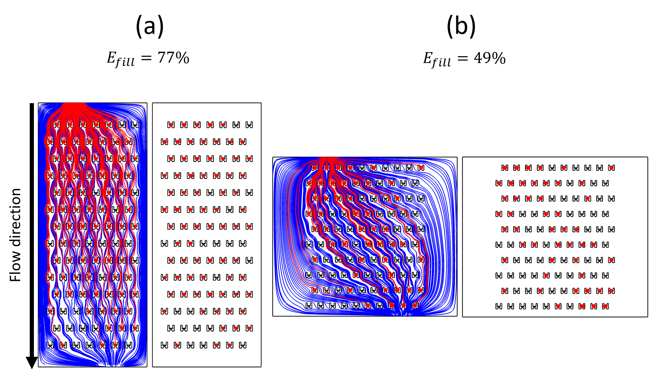
Figure 4: (a) Particle trajectories and final positions for the best geometry resulting from single parametric study. (b) Particle trajectories and final positions for the geometry obtained combining each optimum values from the each parametric study. The corresponding parameter values are: $C=55.5\%$, $W_{r}=64\%$, $L_{r}=90\%$, $A_{r}=1$ and $Wch_{r}=10\%$. The trapped particles and their trajectories are represented in red, the untrapped particle trajectories are represented in blue. The trapped particle diameter is increased to improve readability.

Nonetheless, an optimal inlet/outlet shift is not the same for a different inlet/outlet channel width for example (different $Wch_{r}$). Thus, a simple optimisation approach fixing each parameter to its optimal value from this first study can not result in an efficient geometry. Indeed, the geometry built with each optimum values taken separately exhibits a low filling efficiency ($49\%$) with respect to the current optimal one ($77\%$), see Figure 4b. We deduce that optimisation of MTA-chamber trapping efficiency is a complex and non-intuitive process and is about finding a compromise between combinations of geometric parameters which justifies a multiparametric approach.

3.2 Optimisation of a regular trap array

In this section, the MTA is let as staggered and several optimisation algorithms are coupled with the numerical model. The optimisation problem consists in finding optimal set of parameter values leading to a maximum of an objective function. For implementation simplicity, we defined the optimisation objective function as capture efficiency: $E_{capt}(C,W_{r},L_{r},A_{r},Wch_{r})$. The optimisation results should also be optimal in filling efficiency due to the strong correlation between both metrics. To optimise $E_{capt}$, we used two different approaches: local (simplex based Nelder-Mead [36]) and global (Monte-Carlo [37]).

Figure 5a illustrates the local optimisation technique for a single variable objective function (blue curve) having two maxima: $M_{1}$ and $M_{2}$ points. $M_{1}$ is a local but not global maximum of the objective function whilst $M_{2}$ is the global maximum of the objective function. First, an initial set of parameter value is chosen and the objective is calculated: $I_{1}$, $I_{2}$, $I_{3}$ and $I_{4}$ represent $4$ different choices of initial values. A local optimisation algorithm follows the fastest growth of the objective function from the chosen initial point with or without calculating the derivative(s) of the objective function like a blinded walker trying to reach a peak of a mountain chain [38]. Since we have no proof of $E_{capt}$ differentiability with respect to the parameters, we choose a derivative-free method: the simplex-based Nelder-Mead method. Depending on the initial parameter values, the local optimisation algorithm converges towards different maxima: from the $I_{1}$ and $I_{2}$ points, the convergence point is $M_{1}$ whilst from the $I_{3}$ and $I_{4}$ points, the convergence point is $M_{2}$. The main advantage of local optimisation is the low number of model evaluations needed to find an optimum. However, it can stick into local maxima and miss the global maximum.

All the different local optimisations we tried converge towards different local maxima. Thus, we used a global optimisation algorithm (Monte Carlo) which can not stick into local maxima. This technique randomly samples points within a uniform distribution inside the domain of parameters variations specified by us [38]. The convergence of such algorithm is low and not guaranteed. However, since the model has a low computational cost, this method seems appropriate and we limit the number of model evaluation to $2000$ for approximately $1$ day of computation time. As expected, we obtain our best filling efficiency with this algorithm: $E_{fill}=81\%$, which is $4\%$ better than the best geometry obtained by the parametric study (with $E_{fill}=77\%$).

Figure 5b shows the particle trajectories and final positions for the globally optimised geometry. The corresponding parameter values are: $C=44\%$, $W_{r}=78\%$, $L_{r}=87\%$, $A_{r}=50\%$, $Wch_{r}=48\%$. Interestingly, it seems difficult to reach a filling efficiency better than about $81\%$. In addition, the fact that $C\neq 100\%$ confirms the importance of an oblique flow that allows increasing filling efficiency. We believe that the symmetry breaking between the upstream and downstream flow allows a lateral dispersion of the particles. As such, mass transport in the lateral direction of the flow should be improved by adding disorder in the design of the MTA which is the subject of the next section.

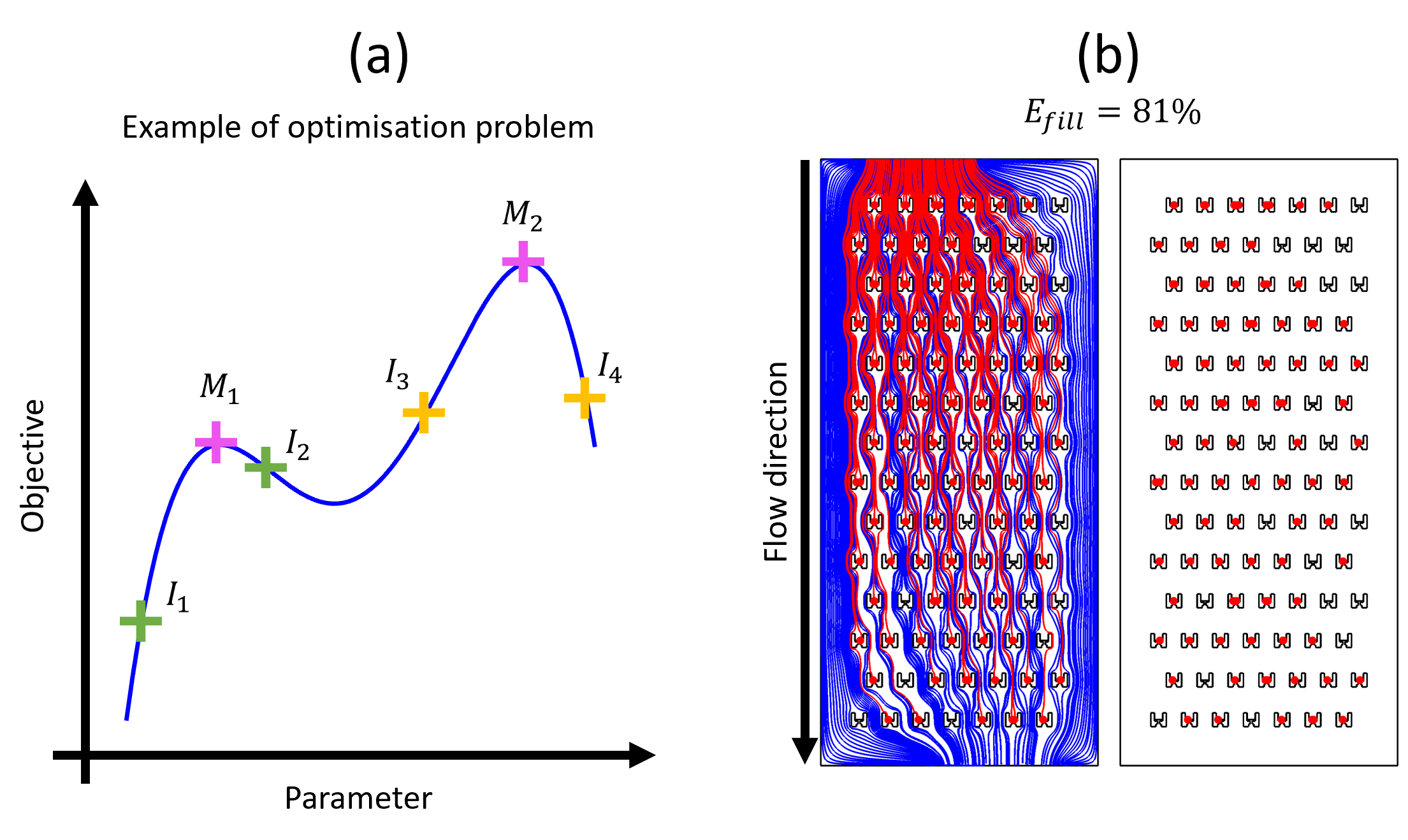
Figure 5: (a) Sketch of the local optimisation principle for a single parameter objective function. $M_{1}$ and $M_{2}$ are maximums of the function. $I_{1}$, $I_{2}$, $I_{3}$ and $I_{4}$ points represent $4$ different choices of initial values. (b) Particle trajectories and final positions in the globally optimised chamber. The trapped particles and their trajectories are represented in red, the untrapped particle trajectories are represented in blue. The trapped particle diameter is increased to improve readability.

3.3 Disorder parametric study

In this section, we investigate how the addition of disorder on the trap positioning may affect filling efficiency. For this purpose, we explore geometries generated as described in section 2.3. The initial geometry is the reference geometry (shown Figure 1) of low filling efficiency ($E_{fill}=51\%$). Disorder is then added in the MTA using $10$ different values of the disorder factor $D_{f}$ introduced in section 2.3. As the MTA geometry is built with probability laws, the repeatability of the results is assessed by rebuilding the geometry $10$ times for each $D_{f}$ value. Figure 6 shows the evolution of $E_{fill}$ with respect to the disorder factor $D_{f}$ for uniform (a) and Gaussian (b) disorders. We notice that for a same $D_{f}$ value (same colour), a variety of different geometries can be obtained, leading to a dispersity of filling efficiency about $15\%$ (bounded by the maximum and minimum values). This random variability should prevent optimisation algorithms to converge. For both disorder distributions, we observe that the mean filling efficiency increases with the disorder parameter and reach a plateau about $\sim 72\%$ (black crosses) at $D_{f}\geq 0.3$ for the uniform and at $D_{f}\geq 0.5$ for the Gaussian disorder. For both disorder distributions, a maximum of filling efficiency is identified to be of $80\%$ (big pink stars) which is very close to the previous one of $81\%$ obtained for the optimisation of a regular MTA. The best geometries are respectively obtained for $D_{f}=0.40$ and $D_{f}=0.64$ for uniform and Gaussian distributions respectively. Therefore, uniform and Gaussian disorders are equally efficient and can reach very similar efficiencies as an optimised oblique chamber with a staggered trap array.

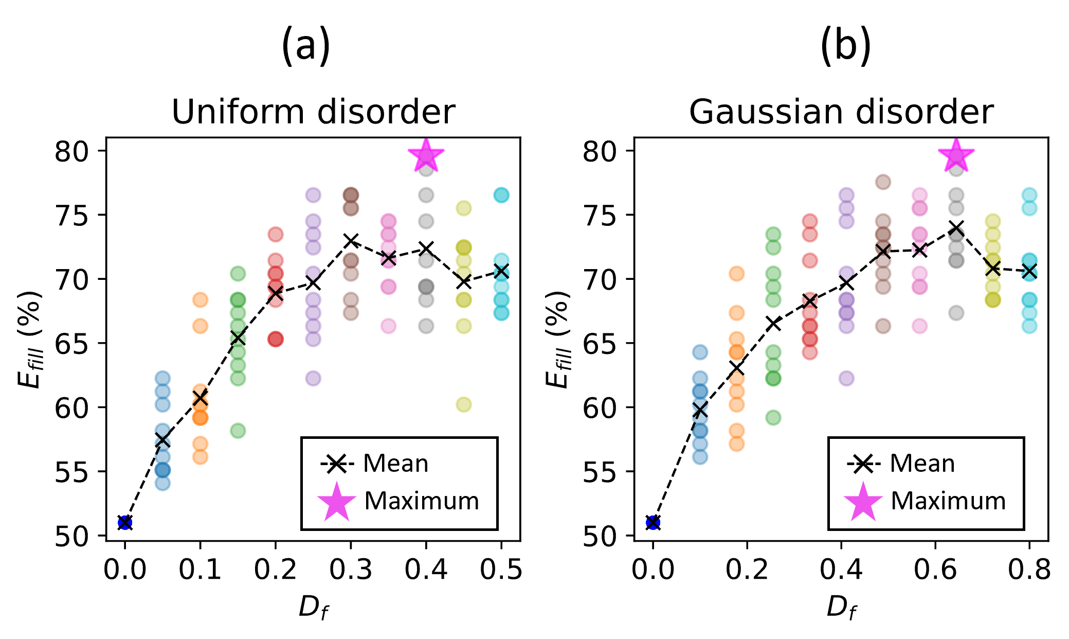
Figure 6: Evolution of filling efficiency in a disordered MTA with a symmetric cavity (same cavity as in Figure 1) with respect to a uniform (a) and a Gaussian distribution (b) of the disorder factor $D_{f}$. Each simulation is represented by a dot. For each $D_{f}$ value, the geometry is re-built $10$ times, which corresponds to a fixed colour of vertically aligned dots. Dot colour appears darker when several point overlaps i.e when several simulation results are equal in filling efficiency for a same $D_{f}$ value. Black crosses represent the mean of $E_{fill}$ values for each $D_{f}$ value. Black crosses are connected by dashed lines to improve visibility.

Figure 7 shows the particle trajectories and final positions for the symmetric reference chamber (a), the best uniform (b) and best Gaussian (c) distributions of the disorder factor. In order to identify trapped particles, these are represented in red, while those that are not trapped are indicated in blue. The respective filling efficiencies are $51\%$ (reference geometry) and $80\%$ for both uniform and Gaussian disorders (corresponding to the big pink stars Figure 6a,b).

In a symmetric chamber where inlet and outlet channels are perfectly aligned, streamlines exhibit upstream/downstream symmetry along the traps far enough from the inlet and outlet (Figure 7a). Therefore, the first trap rows are filled by the particles in the flow direction and almost all the next trap rows stay empty. Then, non-trapped particles display zigzag-like trajectories around the traps, see zoom of Figure 7a. Breaking the upstream/downstream flow symmetry thanks to the addition of disorder modify the symmetric streamline patterns and allows a spanwise mass transport up to eventually filling a next trap. For optimised oblique MTAs, this spanwise mass transport is provided by the shift between the inlet and the outlet channels. A symmetry breaking of upstream/downstream streamlines in disordered MTA is also clearly visible in the zooms of Figure 7b and 7c. Indeed, a saddle point appears on the upstream side of the trap, and streamlines recombine downstream. By breaking the symmetry, streamlines may explore traps in the lateral direction, a possibility that would not have been possible with a staggered trap array. Therefore, we think that lateral dispersion is a key mecanism allowing flow symmetry breaking and then particle trapping. Such phenomenon should be quantitatively investigated which is the subject of the next section.

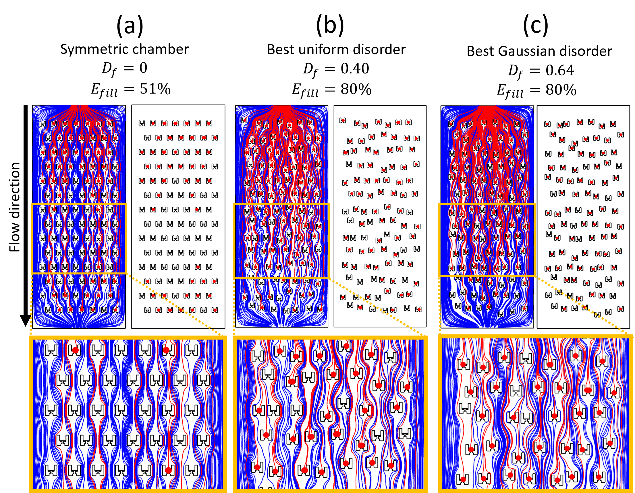
Figure 7: Particle trajectories and final positions in a symmetric chamber (a), the disordered chamber for the best uniform (b) and Gaussian (c) distributions. The trapped particles and their trajectories are represented in red, the untrapped particle trajectories are represented in blue. The trapped particle diameter is increased to improve readability.

Before this quantitative analysis, we would like to point a remark: the significant increase of filling efficiency is not observed when adding disorder to the optimised oblique cavity presented in previous section (see supplementary section S2.2). In this case, filling efficiency stagnates in average and the best filling efficiency is $78\%$ (see supplementary Figure S2a), which is close to the best filling efficiencies obtained so far of $80\%$, Figure 7b). Therefore, we think that uniform disorder allows to maintain approximately $80\%$ of filling efficiency independently of the cavity geometry. We can take advantage of this independence to increase the size of the trap array in the lateral direction at will (see supplementary section S2.3).

3.4 How lateral dispersion influences trapping efficiency

Figure 8 illustrates the principle of particle dispersion. Figure 8a is a sketch of the particle positions in the chamber. At $t=t_{0}$, particles are regularly distributed at the inlet. At $t=t_{1}$, the obstacles (black squares representing the traps) modify the distances between each initially adjacent particles in the flow direction (along $x$) and in the lateral direction (along $y$). At $t=t_{2}$, the dispersion still evolves due to the irregular obstacle positions. Figure 8b shows how we calculate particle dispersion. For every time step $t$ and for each pair of initially adjacent particles (here we take the example of the purple and light green particles), we calculate the distance between particles in the lateral direction $d_{\perp}$ (red double arrow). Lateral dispersion is represented by the statistics of $d_{\perp}$ and more precisely by the mean square lateral distance $\sigma_{\perp}^{2}=\langle d_{\perp}^{2}\rangle-\langle d_{\perp}\rangle^{2}$ where $\langle.\rangle$ represents the average operation over the population of particle pairs. The statistics is made on $2\times\rm{number\ of\ traps}-1$ particle pairs.

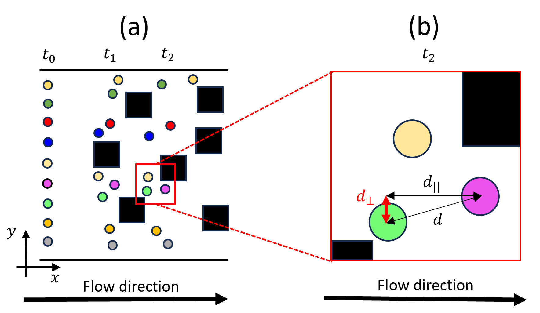
Figure 8: Principle of particle dispersion. (a) Sketch illustrating particle dispersion in the microfluidic chamber. Each particle is identified by a specific colour. Time steps sorted in ascending order are $t_{0}$, $t_{1}$ and $t_{2}$. Black squares represent an obstacle network (the traps in this study). (b) Enlarged view of the sketch representing the quantity of interest we calculate from the simulation results: the lateral distance between particles $d_{\perp}$ (thick red double arrow). The other distances $d$ (total) and $d_{||}$ (streamwise) include particle dispersion in the flow direction which does not participate to trapping phenomena.

We study the particle lateral dispersion in three cases with $800$ traps MTAs having an homothetic cavity than the previous ones: symmetric chamber (with wide inlet/outlet channels), globally optimised oblique chamber and disordered chamber starting with a symmetric cavity ($D_{f}=0.40$ and uniform distribution with wide inlet/outlet channels). The results are plotted on Figure 9.

Lateral mean square distance $\sigma_{\perp}^{2}$ evolves in a comprehensive way with respect to filling efficiency (Figure 9a): interestingly, it seems to reach an asymptotic value for the symmetric chamber at the larger times (blue curve) while the values continue to increase for the disordered and oblique chambers (red and green curves). More precisely, the asymptote of $\sigma_{\perp}^{2}$ for the symmetric chamber is associated with a steady histogram of lateral distance between couples of particles visible Figure 9b: the green distribution (at $t=5$ s) is almost the same as the blue distribution (at $t=7$ s) of $d_{\perp}$. Conversely, the same histograms for oblique (Figure 9c) and disordered chambers (Figure 9d) continue to spread with time. The absence of $\sigma_{\perp}^{2}$ saturation for the oblique and disordered cases is in agreement with our expectation: both flows continuously disperse particles in the lateral direction which explains why no empty region appears in the middle of both chambers (see Figures 5a and 7b). Therefore, we believe the lateral mean square distance $\sigma_{\perp}^{2}$, is a reliable quantity to anticipate MTA’s filling efficiency.

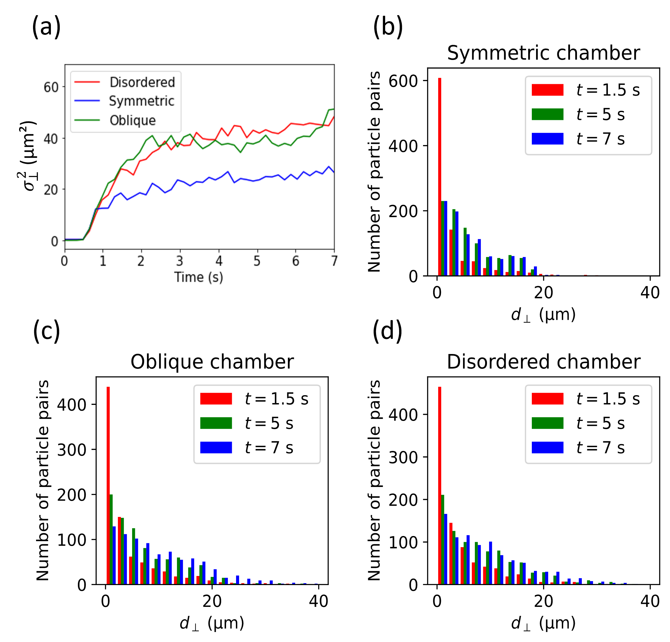
Figure 9: (a) Lateral dispersion regime in the three tested chambers for a $800$ traps MTA. Blue curve for the symmetric chamber, green for the optimised oblique and red for the disordered chamber. After $7$ s, some particles reach the chamber outlet. Histograms of the lateral distance between particle couples at three instants ($1.5$ s, $5$ s and $7$ s) for the symmetric chamber (b), the optimised oblique chamber (c) and the disordered chamber (d).

3.5 Preliminary experimental verification

Since the efficiency of oblique flows was already proved experimentally with PS beads, droplets [14] and utilised for biological applications [6], we focus on the disordered chamber. The associated trapping experiments were conducted in a uniformly disordered chamber with $D_{f}=0.3$. At this value, the saturation of filling efficiency is reached (Figure 6a). The fabricated chamber is shown Figure 10(a). Figure 10b shows the progressive loading of the experimental MTA, a stationary filling is reached in $60$ s of loading. From these images and ImageJ ®, we create a binar matrix of the MTA which allows to easily calculate the experimental filling efficiency (Figure 10c). As expected, the filling efficiency is high: $(E_{fill})_{exp}=81\%$ and in the same order as expected for the optimised disordered geometry.

Figure 10: Trapping experiment results in disordered MTA. (a) PDMS fabricated chamber following standard photolithography process. (b) Fluorescence microscopy images of the MTA progressive loading with $5$ µm polystyrene beads. (c) Filling matrix of the experiment, white colour corresponds to empty traps and blue for occupied traps.

4 Conclusion

In this study, we investigated the trapping efficiency in dense single layer MTAs. We adapted our previously presented CFD/particle model to parametrically optimise the filling efficiency with five dimensionless geometric parameters. After confirming that each parameter influences the capture and filling efficiencies, we used different algorithmic optimisation approaches (local and global) on a regular trap array. The results show the importance of creating an oblique flow to increase filling efficiency. These oblique flows break the upstream/downstream symmetry of the traps and thus enhance transverse dispersion of the particles. We show that this symmetry breaking is accompanied by an increase in lateral dispersion, favouring particle exploration over a wider area. While improving lateral dispersion is a critical point in favouring trap filling, we have shown that it is also possible to introduce disorder into the trap paving. The advantage of this configuration is that is does not constrain the cavity and inlet/outlet geometry for similar filling efficiencies than an optimised oblique flow geometry. A preliminary experimental study confirmed the efficiency of disordered trap arrays on one example, demonstrating the relevance of the approach. We think that further experimental investigations on very large MTAs should finally reveal which geometry is the most interesting.

5 Acknowledgements

This work has received support from the administrative and technological staff of “Institut Pierre-Gilles de Gennes” (Laboratoire d’excellence : ANR-$10$-LABX-$31$, “Investissements d’avenir” : ANR-$10$-IDEX-$0001$-$02$ PSL and Equipement d’excellence : ANR-$10$-EQPX-$34$). NR acknowledges funding from the École Normale Supérieure de Rennes (ENS Rennes, Contrat Doctoral Spécifique Normalien) for PhD scholarship. MCJ acknowledges CNRS and Université de Rennes for financial support.

6 Author contributions

Concepts were proposed by MCJ and JF. Data curation was done by NR and formal analysis by MCJ and NR. Simulations were performed by NR, experiments were conducted by GF (fabrication, trapping) and NR (trapping). NR, MCJ and JF built the methodology and interpreted the results. The manuscript was written by NR and reviewed for scientific and technical aspects by MCJ and JF and for formal aspects by MCJ and RA. Work were supervised by MCJ, JF and RA. Access to simulation material was supported by RA.

7 Conflicts of interest

There are no conflicts of interest to declare.

S1 Supplementary information: Materials and Method

S1.1 Model parameters values

The numerical parameters used in the model are reported in the following Table S1.

Fixed geometric parameters	Description	Value
$h$	chamber’s out-of-plane depth	$14$ µm
$w_{o}$	Traps small opening width	$4$ µm
$w_{pil}$	Trap pillar width	$7$ µm
$w_{sr}$	Traps small rectangle width	$10$ µm
$w_{trap}$	Traps width	$30$ µm
$\Delta x$	Horizontal distance between traps	$50$ µm
$\Delta y$	Vertical distance between traps	$30$ µm
$l_{sr}$	Trap small rectangle’s length	$5$ µm
$l_{trap}$	Trap’s length	$27$ µm
$N_{traps}$	Number of traps in the MTA	$96-98$
Physical parameters	Description	Values
$\mu$	Fluid dynamic viscosity	$0.001$ Pa s
$N_{part}$	Number of particles	$2\ N_{traps}$
$p_{in}$	Uniform inlet pressure	$100$ Pa
$p_{out}$	Uniform outlet pressure	$0$ Pa
$\rho$	Fluid density	$1000$ kg m-3
$R_{p}$	Particles radius	$2.5$ µm
$T_{e}$	Study time	$3$ s - $32$ s
Parametric & optimisation studies	Description	Values
$C$	Inlet/outlet centering	$[0,100]\ \%$
$W_{r}$	Width ratio	$[55,95]\ \%$
$L_{r}$	Length ratio	$[55,95]\ \%$
$A_{r}$	Aspect ratio	$0.3$,$0.4$,$0.5$,$0.7$,$1$,$1.5$,$2$,$2.7$,$3.8$
$Wch_{r}$	Channel to chamber width ratio	$[10,100]\ \%$

Table S1: The model parameters. For single parametric studies, $10$ parameters values are chosen to uniformly vary in the specified interval excepted for the $A_{r}$ parameter where $9$ values are chosen to have the same total number of traps $\pm 3$ traps.

S1.2 Finite-Element implementation

In COMSOL, the Brinkman equation is written in the classical Continuum Mechanics formulation :

$$\begin{cases}\nabla.\mbox{$\underline{\underline{\sigma}}$}+\underline{f}=\underline{0}\\ \nabla.\underline{v}=0\\ \mbox{$\underline{\underline{\sigma}}$}=-p\mbox{$\underline{\underline{I}}$}+2\mu\mbox{$\underline{\underline{D}}$}\\ \mbox{$\underline{\underline{D}}$}=\dfrac{1}{2}\left(\nabla\underline{v}+(\nabla\underline{v})^{T}\right)\\ \end{cases}$$ (12)

where $\underline{\underline{\sigma}}$ is the Newtonian fluid Cauchy stress tensor, $\underline{\underline{I}}$ the identity tensor and $\underline{\underline{D}}$ the strain rate tensor. The mixed weak form equation implemented in COMSOL is obtained by applying the scalar product of Brinkman equation with test velocity $\hat{\underline{v}}$ and by multiplying the mass-conservation (continuity) equation by test pressure $\hat{p}$ and then integration on the fluid domain $\Omega$ (grey domain Figure 1):

$$\begin{cases}\begin{aligned} \int_{\Omega}\;\end{aligned}{(\nabla.\mbox{$\underline{\underline{\sigma}}$}).\hat{\underline{v}}}\ d\Omega+\begin{aligned} \int_{\Omega}\;\end{aligned}{\underline{f}.\hat{\underline{v}}}\ d\Omega=0\\ \begin{aligned} \int_{\Omega}\;\end{aligned}{\hat{p}\nabla.\underline{v}}\ d\Omega=0\\ \end{cases}$$ (13)

Then by integration by part of the first integral and application of Green-Ostrogradski theorem, the following weak form is implemented into COMSOL :

$$\begin{cases}\begin{aligned} \int_{\Omega}\;\end{aligned}{-\mbox{$\underline{\underline{\sigma}}$}:\nabla\hat{\underline{v}}}\ d\Omega+\begin{aligned} \oint_{\partial\Omega}\;\end{aligned}{(\mbox{$\underline{\underline{\sigma}}$}\ \underline{n}).\hat{\underline{v}}}\ d\Gamma+\begin{aligned} \int_{\Omega}\;\end{aligned}{\underline{f}.\hat{\underline{v}}}\ d\Omega=0\\ \begin{aligned} \int_{\Omega}\;\end{aligned}{\hat{p}\nabla.\underline{v}}\ d\Omega=0\\ \end{cases}$$ (14)

Where the first integral represents the virtual power of internal forces including viscous and pressure forces. The second term represents the virtual power of boundary external forces not null only on the inlet and outlet boundaries where the pressure is prescribed and where $\hat{\underline{v}}$ is not null. The last term represents the virtual power of external body forces. The latter equations are discretised in space by applying the Finite-Element Method (FEM) with linear Lagrange shape functions for both pressure and velocity fields (P$1$/P$1$ elements). Even without advection term, such elements must be stabilised to satisfy Ladyzhenskaya–Babuška–Brezzi (LBB) condition. To do so, the COMSOL consistent streamline stabilisation term is added. The weak form equation discretisation is obtained first by applying the nodal (Galerkin) interpolation for $\underline{v}$ and $p$ by their respective interpolation functions and then by replacing the test functions by all interpolation functions. The resulting linear system of equations is numerically inverted using the COMSOL MUMPS solver.

S2 Supplementary information: results

S2.1 Cavity comprehensive parametric study: capture efficiency results

The results of the cavity comprehensive parametric study in capture efficiency (ie the proportion of trapped particles defined 2.3) are summarised Figure S1. We notice the very similar curve trends with respect to filling efficiency displayed Figure 3, leading to a $96\%$ linear correlation coefficient between the two metrics (capture and filling efficiencies). As a consequence, the optimum geometry for both metrics is obtained for the same parameter value $C=55.5\%$.

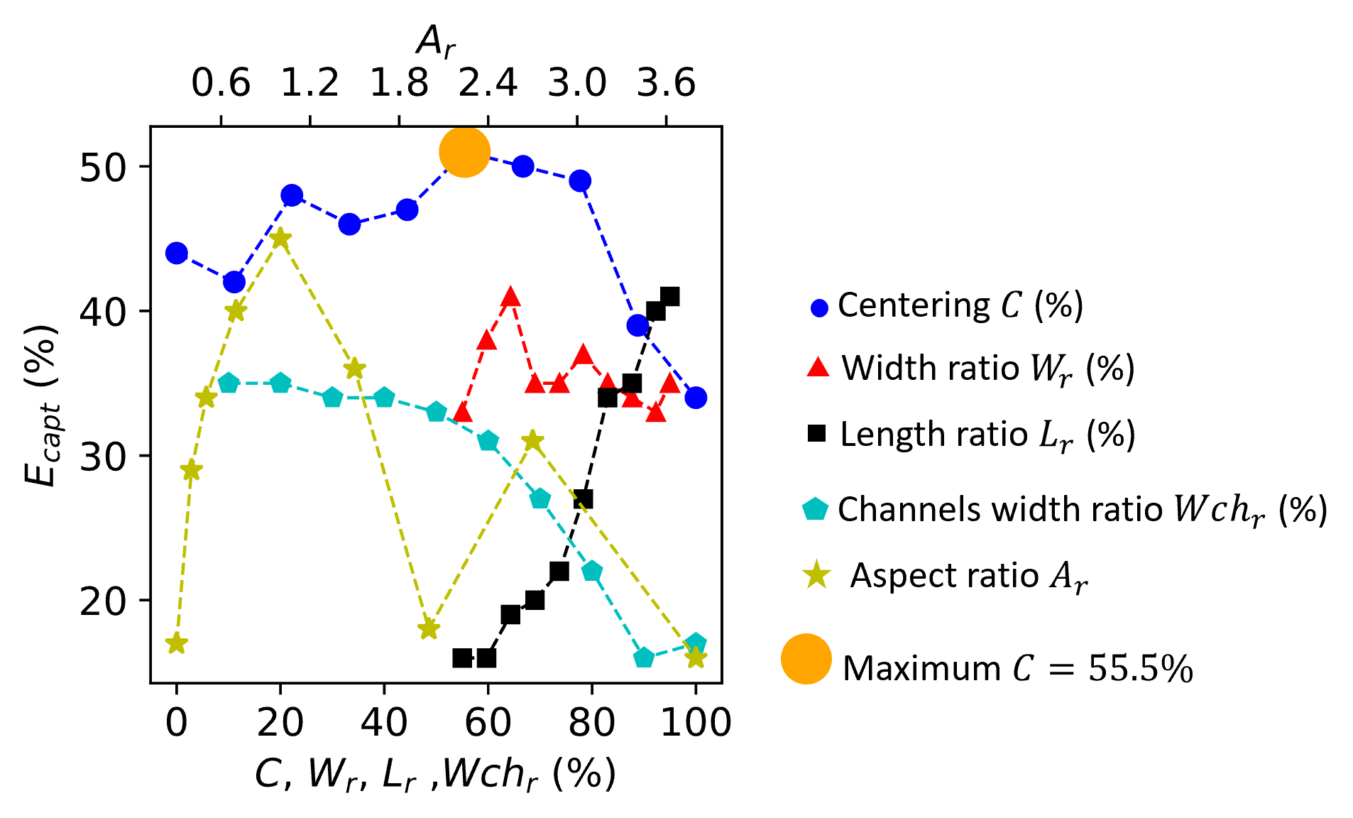
Figure S1: Influence of the five cavity dimensionless parameters $C$, $W_{r}$, $L_{r}$, $A_{r}$ and $Wch_{r}$ on capture efficiency. When parameters are fixed, their respective values are : $C=100\%$, $W_{r}=84\%$, $L_{r}=86\%$, $A_{r}=50\%$ and $Wch_{r}=23\%$ which corresponds to the reference geometry Figure 1. Results from a same parametric study are connected by dashed lines to improve readability.

S2.2 Disorder parametric study for optimised cavity

We study the influence of uniform disorder with the optimised oblique cavity presented section 3.2 and Figure 5b. To do so, we conduct the same disorder factor $D_{f}$ parametric study as in section 3.3: we screen $10$ values of $D_{f}$ with a geometry rebuilt $10$ times for each $D_{f}$ value. Figure S2a shows the evolution of filling efficiency with respect to the disorder factor $D_{f}$. Interestingly, adding disorder slightly decreases filling efficiency because the maximum filling efficiency is obtained without adding disorder: $E_{fill}=81\%$ and the best filling efficiency obtained with a disordered MTA is $E_{fill}=78\%$ (highest dot for $D_{f}=0.5$ Figure S2a). Therefore, the use of disordered trap array seems relevant only with a non-optimised cavity.

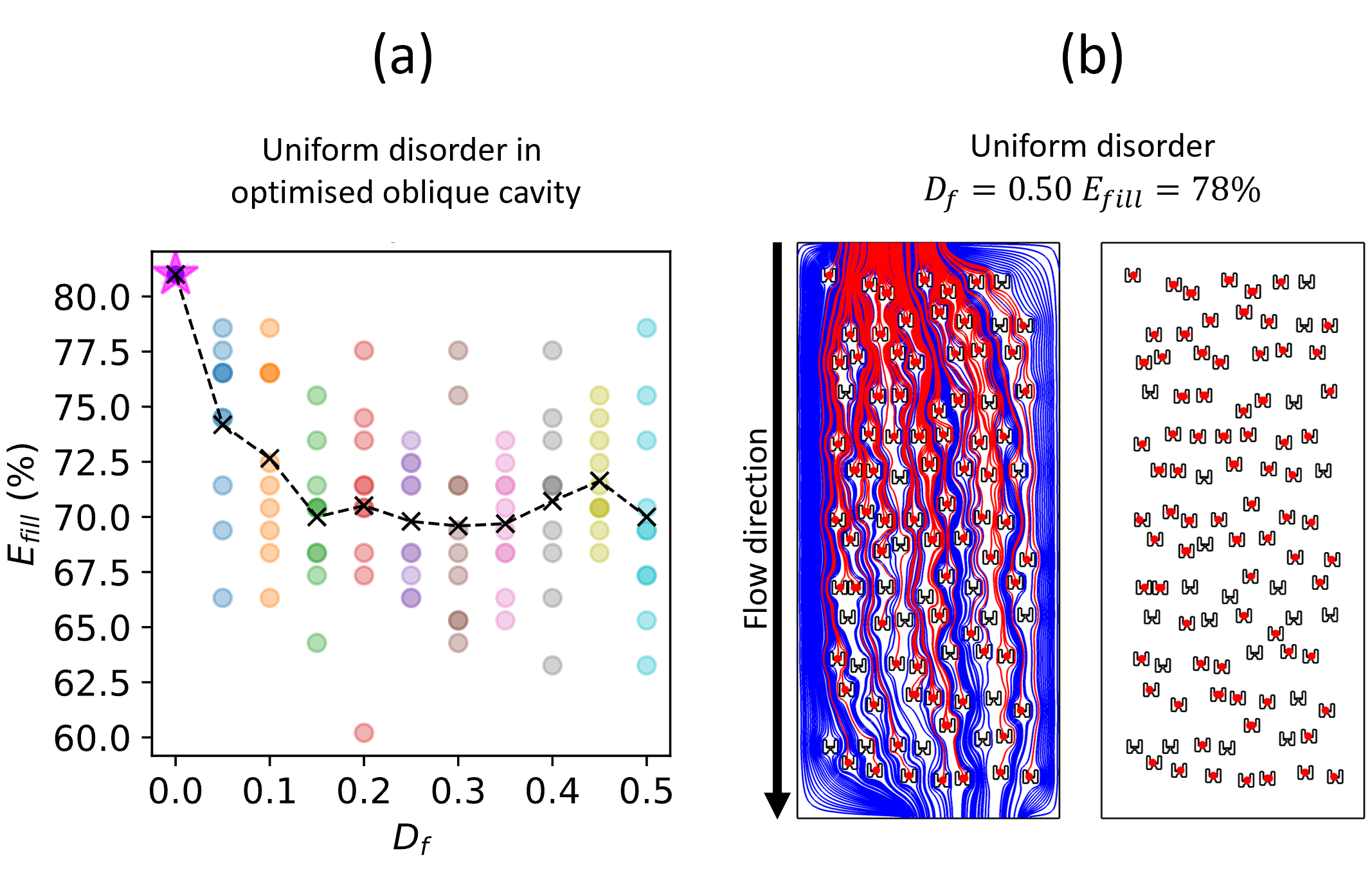
Figure S2: (a) Evolution of capture efficiency with respect to the the disorder factor $D_{f}$ for a uniform disorder. Each simulation is represented by a dot. For each $D_{f}$ value, the geometry is re-built $10$ times, which corresponds to a fixed colour of vertically aligned dots. Dot colour appears darker when several point overlaps i.e when several simulation results are equal in filling efficiency for a same $D_{f}$ value. Black crosses represent the mean of $E_{fill}$ values for each $D_{f}$ value. Dark crosses are connected by dashed lines to improve readability. (b) Particle trajectories and final positions for the most efficient disordered trap array with the optimised oblique cavity (corresponding to the highest point of Panel (a) with $D_{f}=0.50$). The trapped particles and their trajectories are represented in red, the untrapped particle trajectories are represented in blue. The trapped particle diameter is increased to improve readability.

S2.3 Disordered trap arrays can be easily expanded in the lateral direction

Disordered MTAs generate lateral dispersion of particles due to the trap relative positions. This characteristic offers more possibilities of the inlet/outlet channels and cavity designs than an optimised oblique chamber where all the five dimensionless parameters are fixed. As an example, we show here that when using the largest possible inlet/outlet channels ($Wch_{r}=100\%$) and expanding the MTA size in the lateral direction, the filling and capture efficiencies are few modified and the averaged filling efficiency remains very close to $80\%$ (Figure S3a) even though the MTA aspect ratio $A_{r}$ and width ratio $W_{r}$ are modified. The particle trajectories corresponding to largest chamber are shown Figure S3b.

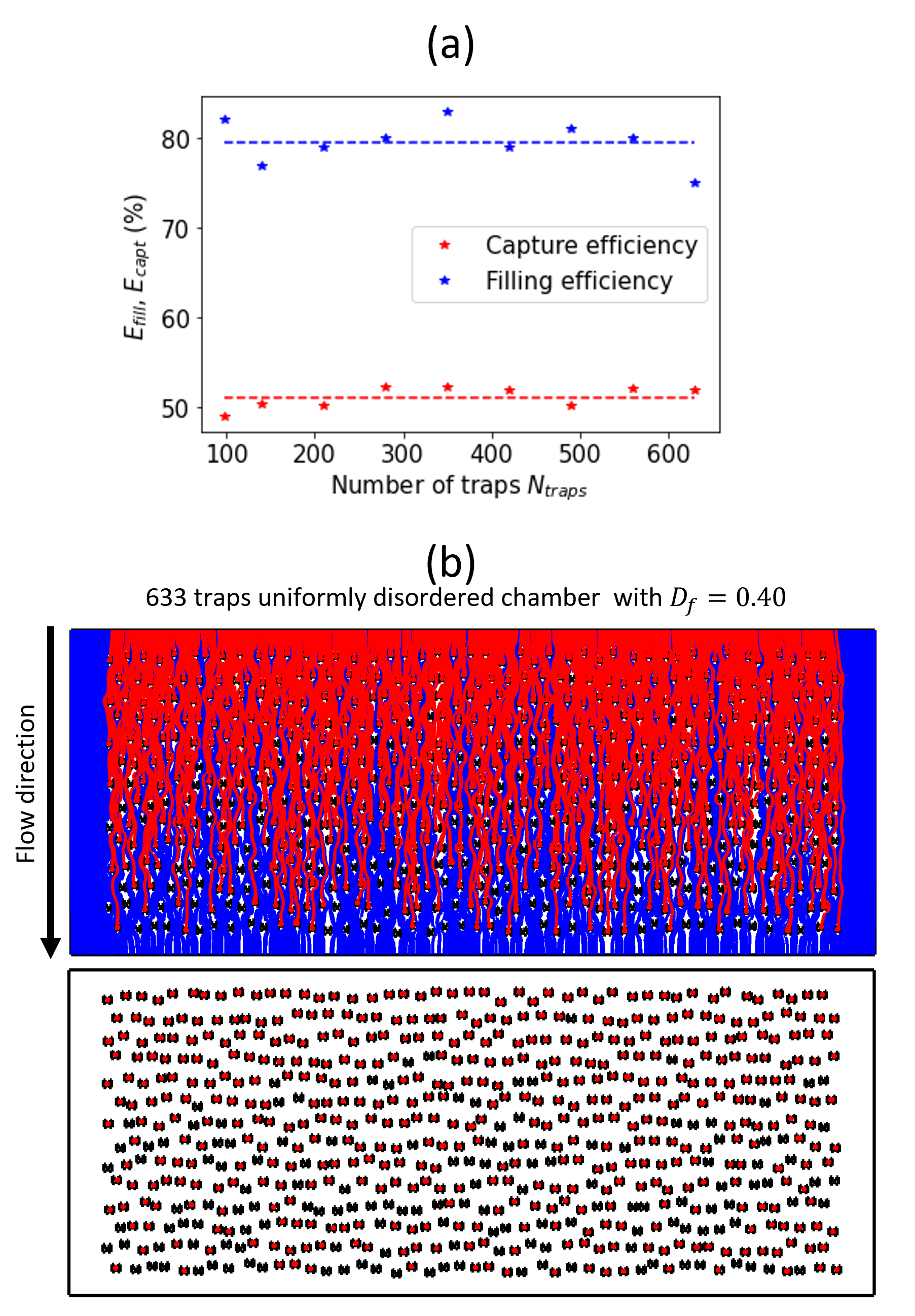
Figure S3: (a) Evolution of capture and filling efficiencies with respect to the number of traps when laterally expanding a $D_{f}=0.40$ uniformly disordered MTA. Horizontal lines correspond to constant function least square fittings. (b) Particles trajectories in the biggest disordered MTA simulated on Panel (a). The trapped particles and their trajectories are represented in red, the untrapped particle trajectories are represented in blue. The trapped particle diameter is increased to improve readability.

References

- Wlodkowic and Cooper [2010] Donald Wlodkowic and Jonathan M. Cooper. Microfluidic cell arrays in tumor analysis: New prospects for integrated cytomics. Expert Review of Molecular Diagnostics, 10(4):521–530, 2010. ISSN 14737159. doi: 10.1586/erm.10.28.
- Dereli-Korkut et al. [2014] Zeynep Dereli-Korkut, H. Dogus Akaydin, A. H.Rezwanuddin Ahmed, Xuejun Jiang, and Sihong Wang. Three dimensional microfluidic cell arrays for ex vivo drug screening with mimicked vascular flow. Analytical Chemistry, 86(6):2997–3004, 2014. ISSN 15206882. doi: 10.1021/ac403899j.
- Lee et al. [2008] Philip J. Lee, Noah C. Helman, Wendell A. Lim, and Paul J. Hung. A microfluidic system for dynamic yeast cell imaging. BioTechniques, 44(1):91–95, 2008. ISSN 07366205. doi: 10.2144/000112673.
- Jackson-Holmes et al. [2017] E. L. Jackson-Holmes, T. C. McDevitt, and H. Lu. A microfluidic trap array for longitudinal monitoring and multi-modal phenotypic analysis of individual stem cell aggregates. Lab on a Chip, 17:3634–3642, 11 2017. ISSN 14730189. doi: 10.1039/c7lc00763a.
- Pinon et al. [2022] Léa Pinon, Nicolas Ruyssen, Judith Pineau, Olivier Mesdjian, Damien Cuvelier, Anna Chipont, Rachele Allena, Coralie L. Guerin, Sophie Asnacios, Atef Asnacios, Paolo Pierobon, and Jacques Fattaccioli. Phenotyping polarization dynamics of immune cells using a lipid droplet-cell pairing microfluidic platform. Cell Reports Methods, page 100335, 2022. ISSN 26672375. doi: 10.1016/j.crmeth.2022.100335.
- Pineau et al. [2022] Judith Pineau, Léa Pinon, Olivier Mesdjian, Jacques Fattaccioli, Ana-Maria Lennon-Duménil, and Paolo Pierobon. Microtubules restrict F-actin polymerization to the immune synapse via GEF-H1 to maintain polarity in lymphocytes. Elife, 11, 2022. doi: 10.7554/elife.78330.
- Di Carlo et al. [2006] Dino Di Carlo, Nima Aghdam, and Luke P. Lee. Single-cell enzyme concentrations, kinetics, and inhibition analysis using high-density hydrodynamic cell isolation arrays. Analytical Chemistry, 78(14):4925–4930, 2006. ISSN 00032700. doi: 10.1021/ac060541s.
- Skelley et al. [2009] Alison M. Skelley, Oktay Kirak, Heikyung Suh, Rudolf Jaenisch, and Joel Voldman. Microfluidic control of cell pairing and fusion. Nature Methods, 6(2):147–152, 2009. ISSN 15487091. doi: 10.1038/nmeth.1290.
- Wlodkowic et al. [2009] Donald Wlodkowic, Shannon Faley, Michele Zagnoni, John P. Wikswo, and Jonathan M. Cooper. Microfluidic single-cell array cytometry for the analysis of tumor apoptosis. Analytical Chemistry, 81(13):5517–5523, 2009. ISSN 00032700. doi: 10.1021/ac9008463.
- Challier et al. [2021] Lylian Challier, Justin Lemarchand, Catherine Deanno, Cecile Jauzein, Giorgio Mattana, Guillaume Mériguet, Benjamin Rotenberg, and Vincent Noël. Printed dielectrophoretic electrode-based continuous flow microfluidic systems for particles 3d-trapping. Particle and Particle Systems Characterization, 38, 2 2021. ISSN 15214117. doi: 10.1002/ppsc.202000235.
- Pompano et al. [2011] Rebecca R. Pompano, Weishan Liu, Wenbin Du, and Rustem F. Ismagilov. Microfluidics using spatially defined arrays of droplets in one, two, and three dimensions. Annual Review of Analytical Chemistry, 4:59–81, 2011. ISSN 19361327. doi: 10.1146/annurev.anchem.012809.102303.
- Carreras and Wang [2017] Maria Pilar Carreras and Sihong Wang. A multifunctional microfluidic platform for generation, trapping and release of droplets in a double laminar flow. Journal of Biotechnology, 251:106–111, 2017. ISSN 18734863. doi: 10.1016/j.jbiotec.2017.04.030.
- Bai et al. [2010] Yunpeng Bai, Ximin He, Dingsheng Liu, Santoshkumar N. Patil, Dan Bratton, Ansgar Huebner, Florian Hollfelder, Chris Abell, and Wilhelm T.S. Huck. A double droplet trap system for studying mass transport across a droplet-droplet interface. Lab on a Chip, 10:1281–1285, 2010. ISSN 14730189. doi: 10.1039/b925133b.
- Mesdjian et al. [2021] O. Mesdjian, N. Ruyssen, M. C. Jullien, R. Allena, and J. Fattaccioli. Enhancing the capture efficiency and homogeneity of single-layer flow-through trapping microfluidic devices using oblique hydrodynamic streams. Microfluid. Nanofluidics, 25(11):1–11, 2021. ISSN 16134990. doi: 10.1007/s10404-021-02492-1.
- Fradet et al. [2011] Etienne Fradet, Craig McDougall, Paul Abbyad, Rémi Dangla, David McGloin, and Charles N. Baroud. Combining rails and anchors with laser forcing for selective manipulation within 2D droplet arrays. Lab on a Chip, 11(24):4228–4234, 2011. ISSN 14730189. doi: 10.1039/c1lc20541b.
- Sohrabi Kashani and Packirisamy [2019] Ahmad Sohrabi Kashani and Muthukumaran Packirisamy. Efficient Low Shear Flow-based Trapping of Biological Entities. Scientific Reports, 9(1):1–15, 2019. ISSN 20452322. doi: 10.1038/s41598-019-41938-z.
- Charnley et al. [2009] Mirren Charnley, Marcus Textor, Ali Khademhosseini, and Matthias P. Lutolf. Integration column: Microwell arrays for mammalian cell culture. Integrative Biology, 1(11-12):625–634, 2009. ISSN 17579694. doi: 10.1039/b918172p.
- Figueroa et al. [2010] Xavier A. Figueroa, Gregory A. Cooksey, Scott V. Votaw, Lisa F. Horowitz, and Albert Folch. Large-scale investigation of the olfactory receptor space using a microfluidic microwell array. Lab on a Chip, 10:1120–1127, 2010. ISSN 14730189. doi: 10.1039/b920585c.
- Rousset et al. [2017] Nassim Rousset, Frédéric Monet, and Thomas Gervais. Simulation-assisted design of microfluidic sample traps for optimal trapping and culture of non-adherent single cells, tissues, and spheroids. Scientific Reports, 7(1):1–12, 2017. ISSN 20452322. doi: 10.1038/s41598-017-00229-1.
- Winkleman et al. [2004] Adam Winkleman, Katherine L. Gudiksen, Declan Ryan, George M. Whitesides, Derek Greenfield, and Mara Prentiss. A magnetic trap for living cells suspended in a paramagnetic buffer. Applied Physics Letters, 85:2411–2413, 9 2004. ISSN 00036951. doi: 10.1063/1.1794372.
- Smistrup et al. [2006] Kristian Smistrup, Torsten Lund-Olesen, Mikkel F. Hansen, and Peter T. Tang. Microfluidic magnetic separator using an array of soft magnetic elements. Journal of Applied Physics, 99, 2006. ISSN 00218979. doi: 10.1063/1.2159418.
- Zhou et al. [2016] Ying Zhou, Srinjan Basu, Kai J. Wohlfahrt, Steven F. Lee, David Klenerman, Ernest D. Laue, and Ashwin A. Seshia. A microfluidic platform for trapping, releasing and super-resolution imaging of single cells. Sensors and Actuators, B: Chemical, 232:680–691, 2016. ISSN 09254005. doi: 10.1016/j.snb.2016.03.131.
- Au et al. [2011] Anthony K. Au, Hoyin Lai, Ben R. Utela, and Albert Folch. Microvalves and micropumps for BioMEMS, volume 2. Molecular Diversity Preservation International (MDPI), 2011. ISBN 1206616903. doi: 10.3390/mi2020179.
- Grigorenko et al. [2008] A. N. Grigorenko, N. W. Roberts, M. R. Dickinson, and Y. Zhang. Nanometric optical tweezers based on nanostructured substrates. Nature Photonics, 2:365–370, 6 2008. ISSN 17494885. doi: 10.1038/nphoton.2008.78.
- Rosenthal and Voldman [2005] Adam Rosenthal and Joel Voldman. Dielectrophoretic traps for single-particle patterning. Biophysical Journal, 88:2193–2205, 2005. ISSN 00063495. doi: 10.1529/biophysj.104.049684.
- Lee et al. [2004] H. Lee, A. M. Purdon, and R. M. Westervelt. Manipulation of biological cells using a microelectromagnet matrix. Applied Physics Letters, 85:1063–1065, 8 2004. ISSN 00036951. doi: 10.1063/1.1776339.
- Evander et al. [2007] Mikael Evander, Linda Johansson, Tobias Lilliehorn, Jure Piskur, Magnus Lindvall, Stefan Johansson, Monica Almqvist, Thomas Laurell, and Johan Nilsson. Noninvasive acoustic cell trapping in a microfluidic perfusion system for online bioassays. Analytical Chemistry, 79:2984–2991, 4 2007. ISSN 00032700. doi: 10.1021/ac061576v.
- Kobel et al. [2010] Stefan Kobel, Ana Valero, Jonas Latt, Philippe Renaud, and Matthias Lutolf. Optimization of microfluidic single cell trapping for long-term on-chip culture. Lab on a Chip, 10(7):857–863, 2010. ISSN 14730189. doi: 10.1039/b918055a.
- Deng et al. [2014] B. Deng, X. F. Li, D. Y. Chen, L. D. You, J. B. Wang, and J. Chen. Parameter screening in microfluidics based hydrodynamic single-cell trapping. Scientific World Journal, 2014, 2014. ISSN 1537744X. doi: 10.1155/2014/929163.
- Jin et al. [2015] D. Jin, B. Deng, J. X. Li, W. Cai, L. Tu, J. Chen, Q. Wu, and W. H. Wang. A microfluidic device enabling high-efficiency single cell trapping. Biomicrofluidics, 9(1), 2015. ISSN 19321058. doi: 10.1063/1.4905428.
- Xu et al. [2013a] Xiaoxiao Xu, Zhenyu Li, and Arye Nehorai. Finite element simulations of hydrodynamic trapping in microfluidic particle-trap array systems. Biomicrofluidics, 7(5), 2013a. ISSN 19321058. doi: 10.1063/1.4822030.
- Xu et al. [2013b] Xiaoxiao Xu, Pinaki Sarder, Zhenyu Li, and Arye Nehorai. Optimization of microfluidic microsphere-trap arrays. Biomicrofluidics, 7, 2 2013b. ISSN 19321058. doi: 10.1063/1.4793713.
- Wang et al. [2021] Zhiqi Wang, Yuchen Guo, Eddie Wadbro, and Zhenyu Liu. Topology optimization of passive cell traps. Micromachines, 12, 7 2021. ISSN 2072666X. doi: 10.3390/mi12070809.
- Kim et al. [2012] Jeongyun Kim, David Taylor, Nitin Agrawal, Han Wang, Hyunsoo Kim, Arum Han, Kaushal Rege, and Arul Jayaraman. A programmable microfluidic cell array for combinatorial drug screening. Lab on a Chip, 12(10):1813–1822, 2012. ISSN 14730189. doi: 10.1039/c2lc21202a.
- Mottin et al. [2021] Donatien Mottin, Florence Razan, Frédéric Kanoufi, and Marie-Caroline Jullien. Influence of lift forces on particle capture on a functionalized surface. Microfluid. Nanofluid., 25(11):1–10, November 2021. ISSN 1613-4990. doi: 10.1007/s10404-021-02488-x.
- Nelder and Mead [1965] J. A. Nelder and R. Mead. A simplex method for function minimization. The Computer Journal, 7(4):308–313, 01 1965. ISSN 0010-4620. doi: 10.1093/comjnl/7.4.308.
- Multiphysics [2018] Comsol Multiphysics. Optimization module user’s guide. Optimization module User’s guide, Optimization module User’s guide:78, 2018.
- Venter [2010] Gerhard Venter. Review of Optimization Techniques, chapter 2,3, pages 1–10. John Wiley and Sons, Ltd, 2010. ISBN 9780470686652. doi: https://doi.org/10.1002/9780470686652.eae495.