Unravelling the interplay between steel rebar corrosion rate and corrosion-induced cracking of reinforced concrete
Abstract
Accelerated impressed current testing is the most common experimental method for assessing the susceptibility to corrosion-induced cracking, the most prominent challenge to the durability of reinforced concrete structures. Although it is well known that accelerated impressed current tests lead to slower propagation of cracks (with respect to corrosion penetration) than in natural conditions, which results in overestimations of the delamination/spalling time, the origins of this phenomenon have puzzled researchers for more than a quarter of a century. In view of recent experimental findings, it is postulated that the phenomenon can be attributed to the variability of rust composition and density,
specifically to the variable ratio of the mass fractions of iron oxide and iron hydroxide-oxide,
which is affected by the magnitude of the applied corrosion current density. Based on this hypothesis, a corrosion-induced cracking model for virtual impressed-current testing is presented. The simulation results obtained with the proposed model are validated against experimental data, showing good agreement. Importantly, the model can predict corrosion-induced cracking under natural conditions and thus allows for the calculation of a newly proposed crack width slope correction factor, which extrapolates the surface crack width measured during accelerated impressed current tests to corrosion in natural conditions.
keywords:
Reinforced concrete , Impressed current tests , Corrosion-induced cracking , Phase-field fracture , Durability1 Introduction
Corrosion is responsible for premature deterioration of 70-90% of all reinforced concrete structures [1, 2]. One of the most common degradation mechanisms is corrosion-induced cracking, which takes years or decades under natural conditions. For this reason, researchers have strived for decades to accurately simulate and predict corrosion-induced cracking [3].
Currently, there are two methods employed to experimentally simulate corrosion-induced cracking in laboratory conditions [4]. The first option is to expose the concrete specimen to an exaggerated climate, i.e., to various intensities of contact with aggressive species such as chlorides or carbon dioxide, and possibly also to variable humidity (wetting-drying cycles). This accelerates the corrosion process to a certain extent. However, accelerated testing can still require months or years to achieve significant corrosion-induced cracking. Also, corrosion current density, steel mass loss and anodic area are evolving dynamically with the penetration of aggressive species. These are not known in advance and need to be measured in other ways, which often requires many samples to be tested at different stages of the corrosion process.
The other method to simulate corrosion-induced cracking experimentally is the impressed current technique. In this case, an electric potential is applied on the steel rebar which serves as the anode, with typically another stainless steel rebar or mesh serving as the cathode. This method results in nearly uniform corrosion and allows to accurately control corrosion current density and mass loss. At the same time, it allows for applying high corrosion current density in hundreds or thousands of \unit\micro\per\centi^2, which drastically shortens the time of the experiment to days or hours. For all their benefits and simplicity, impressed current techniques have become very popular [3]. However, a major downside is that while corrosion current densities from 100 to 2000 \unit\micro\per\centi^2 are commonly applied in impressed current tests [3], natural corrosion current densities are much smaller, typically about 1 \unit\micro\per\centi^2 [5, 6, 7, 8, 9]. This raises the question of how accurately can the impressed current technique reproduce the corrosion process and corrosion-induced cracking under natural conditions.
To answer this question, Alonso et al. [10] measured the surface crack width on the impressed current test with varying applied corrosion current density and found out that lower current density resulted in faster crack propagation with respect to corrosion penetration (i.e. the thickness of the corroded steel layer). The measured differences were significant: Alonso et al. [10] reported that the slope of linearly fitted crack width/corrosion penetration curve for the corrosion rate of 10 \unit\micro\per\centi^2 was even six times larger than for the corrosion rate of 100 \unit\micro\per\centi^2. The decreasing trend of the slope of linearly fitted crack width/corrosion penetration curves with increasing applied corrosion current density was confirmed by the comprehensive experimental study of Pedrosa and Andrade [11], who found out that the slope is proportional to a negative power of the corrosion current density. Slower propagation of cracks under an increased applied corrosion current density was also observed by Vu et al. [12], Saifullah and Clark [13] and Mullard and Stewart [14] up to approximately 200 \unit\micro\per\centi^2. By fitting the experimental results, Vu et al. [12] proposed a loading correction factor dependent on the applied corrosion current density to allow for the extrapolation of the time to cracking measured within accelerated tests to corrosion in natural conditions. It has to be mentioned that for very high currents over 200 \unit\micro\per\centi^2, some authors reported an increased speed of crack propagation compared to current densities lower than 200 \unit\micro\per\centi^2 [15, 16, 13]. El Maaddawy and Soudki [15] suggested that for a higher corrosion rate, corrosion products have less time to be transported into the concrete pore space and a larger portion of them is thus trapped at the steel-concrete interface, which increases the induced pressure.
Even though the decrease of crack propagation with increasing applied corrosion current up to at least 200 \unit\micro\per\centi^2 is well experimentally documented, there has been no agreement on the origins of this phenomenon. Alonso et al. [10] and Pedrosa and Andrade [11] proposed an alternative explanation, suggesting that the loading rate-dependent material properties of concrete may be responsible. The idea is that the increased strain rate would affect the fracture-related properties such that the tensile strength would increase and delay the cracking process. If this was true, given the range of rates relevant to the corrosion process, the rate-dependency of material properties would have to be caused by creep. Although creep is likely to affect the results of long-term tests conducted under natural-like corrosion current densities, the study of Aldellaa2022a found out that creep alone does not explain the dependence of the speed of the crack propagation (with respect to corrosion penetration) on the corrosion rate.
Recently, a new plausible explanation emerged from the study of Zhang et al. [17] who performed X-ray diffraction (XRD) measurements on the series of rust samples from impressed current tests conducted with different applied corrosion current densities. Zhang et al. [17] found out that the composition of rust, specifically the mass fractions of two main components of rust—iron oxides (mainly wüstite , maghemite and magnetite ) and iron hydroxy-oxides (mainly goethite -FeOOH, akageneite -FeOOH, lepidocrocite -FeOOH)—changed with the applied magnitude of corrosion current. This indicates that as the corrosion current density increases, the mass fraction of iron hydroxy-oxides decreases. Because iron hydroxy-oxides have a smaller density than iron oxides, the decrease in hydroxy-oxide content results in lower corrosion-induced pressures and thus slower crack evolution. Although the study of Liu et al. [18] identified high hydroxy-oxide content even when the corrosion current density was raised to 100 \unit\micro\per\centi^2, the conclusions of Zhang et al. [17] are supported by a number of other experimental studies. Yuan et al. [4] observed different colours (indicating different chemical compositions) of rust produced from accelerated impressed current tests than those corroded in an artificial climate environment closely simulating the natural corrosion process. Chitty et al. [19] investigated rust from ancient Gallo–Roman reinforced concrete artefacts naturally corroding for roughly two millennia and identified mostly hydroxy-oxide goethite with marblings of iron oxides maghemite and magnetite. The analyses of naturally carbonated corrosion products in carbonated reinforced concrete facade panels by Köliö et al. [20] identified mostly hydroxy-oxides goethite, feroxyhite () and lepidocrocite with some rare findings of iron oxides magnetite and maghemite. A very high content (more than 56 mass fraction) of iron oxides in four impressed current tests accelerated to 100 \unit\micro\per\centi^2 was measured by Zhang et al. [21].
These recent findings are adopted to build our hypothesis and develop a corrosion-induced cracking model capable of resolving (i) the reactive transport of dissolved iron species released from the steel surface and their precipitation into the dense rust layer adjacent to the corroding steel surface and the concrete pore space, (ii) the change of the rust chemical composition, specifically the ratio of mass fractions of iron oxides and iron hydroxy-oxides, and thus of the density of rust with the applied magnitude of corrosion current density, (iii) the corrosion-induced pressure of corrosion precipitates accumulating in the dense rust layer and the concrete pore space of concrete, and (iv) the corrosion-induced fracture of concrete, as simulated with a quasi-brittle phase-field fracture model. For the first time, the analytically derived estimates are presented: for (I) the corrosion-induced pressure of the dense layer of corrosion products, which takes into account their compressibility, and (II) the ions flux reduction factor determining the ratio of corrosion products precipitating in the dense rust layer and those transported further into the concrete pore space. Thus, a comprehensive model capable of simulating impressed current tests is provided. Also, the model allows to predict a newly proposed crack width slope correction factor with which the surface crack obtained from impressed current tests can be extrapolated to corrosion in natural conditions.
2 Theory and computational framework
The formulation of the corrosion-induced cracking model comprises several parts. Firstly, the model for reactive transport and precipitation of dissolved iron released from the corroding steel surface is described in Section 2.1, allowing for the prediction of the distribution of iron oxide and iron hydroxy-oxide rust. This is followed by the discussion of the phase-field fracture model in Section 2.2. Corrosion-induced mechanical stress arises from the accumulation of rust in the form of a dense rust layer (Section 2.3) and in the pore space of concrete (Section 2.4). The damage-dependent diffusivity tensor allowing for the consideration of the role of crack in the reactive transport of dissolved iron species is introduced in Section 2.5. The formulation of the model is concluded in Section 2.6 with the summary of governing equations and related boundary conditions.
Notation. Scalar quantities are represented by light-faced italic letters, e.g. , Cartesian vectors by upright bold letters, e.g. , and Cartesian second- and higher-order tensors by bold italic letters, e.g. . The symbol denotes the second-order identity tensor and represents the fourth-order identity tensor. Inner products are denoted by a number of vertically stacked dots, where the number of dots corresponds to the number of indices over which summation takes place, e.g. . Finally, and respectively denote the gradient and divergence operators.
2.1 Reactive transport model
2.1.1 Solution domain, representative volume element (RVE) and primary unknown variables
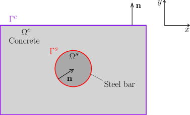
The problem is solved on a domain , which comprises the concrete domain and the embedded steel domain (see Fig. 1). The outer boundary of and is and the inner boundary of between the steel and concrete domains is . The symbol denotes the outer normal vector to the boundary of the concrete domain.
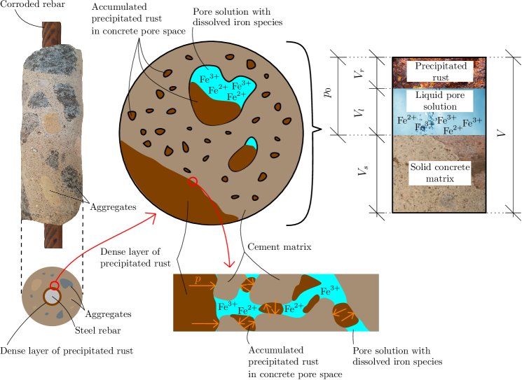
Concrete is a porous material and within the reactive transport model, its internal structure is described by the representative volume element (RVE) depicted in Fig. 2. The concrete RVE of volume is assumed to comprise the solid concrete matrix of volume and the pore space of volume , characterized by capillary porosity , with all these quantities remaining unchanged in time. The pore space is simplified to be fully saturated with water, which is a reasonable assumption in the vicinity of the steel rebar, especially for corrosion induced by impressed current or chloride ingress. There, the pore space is gradually filled with precipitated rust, and the volume of liquid pore solution decreases to the benefit of the increasing volume of precipitated rust . Volume fractions , and saturation ratios , of the liquid pore solution and the precipitated rust provide useful indicators of their current volume content. The primary unknown variables of the reactive transport problem are and , in mols per cubic meter of the liquid pore solution.
2.1.2 Distribution and chemical composition of rust in concrete
Microscopy investigations of corroded reinforced concrete samples [19, 22, 23] show that a portion of the rust accumulates in the immediate vicinity of the corroded steel rebar as a dense rust layer while the remaining rust is located in the concrete pore space up to a certain distance from the rebar (see Fig. 2).
In samples corroded under both natural and accelerated conditions, the main corrosion products found with X-ray diffraction (XRD) measurements were iron oxides (wüstite , hematite , magnetite ) and iron hydroxy-oxides (goethite , akaganeite , lepidocrocite , feroxyhyte ) [19, 24, 17]. It should be noted that the XRD method can determine only the presence of crystalline materials, but some corrosion products are known to be amorphous [24].
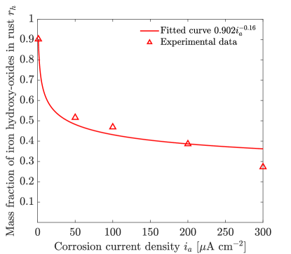
One of the critical inputs of the model is the dependence of the mass fraction of iron hydroxy-oxides in rust on applied corrosion current density because this determines the density of produced rust and thus the induced pressure. This curve is obtained by fitting the experimentally measured data of Zhang et al. [17] with a power function (see Fig. 3), where \unit\micro\per\centi^2 is the reference corrosion current density. The first measurement of Zhang et al. [17] came from a naturally corroded sample for which the value of corrosion current density was not documented and thus it was estimated as 1 \unit\micro\per\centi^2, which is a typical value measured during the natural corrosion process in reinforced concrete [5, 6, 7, 8, 9]. Even though experimental measurements of the mass ratio of particular corrosion products are very scarce in the current literature, the results of Zhang et al. [17] agree with the studies on samples corroded under natural conditions [19, 20] and with accelerated impressed current tests [21]. In Fig. 3one can see that drops dramatically from 0.9 for 1 \unit\micro\per\centi^2 to roughly 0.5 for 50 \unit\micro\per\centi^2, while a subsequent decrease is significantly more moderate.
2.1.3 Iron ion transport and precipitation
An alkaline concrete pore solution allows for the formation of a nanometre-thick protective semiconductive layer on the steel rebar surface, which significantly impedes the corrosion process. However, this layer can be disrupted, typically by chlorides or due to the carbonation of concrete. If water and oxygen are present, corrosion can initiate. A corrosion current of density starts to flow between anodic and cathodic regions and ions are released from the steel surface into the pore solution by reaction (1a). The dissolved ferrous ions then undergo a series of complex chemical reactions forming a number of intermediary products, see for instance [25, 26] for more details. For the purpose of mechanical modelling, the complexity of the chemical reaction system is reduced to three arguably critical reactions (see Fig. 4). The first considered option for ions is to be oxidised to ions (reaction (1b)), which then further precipitate into iron hydroxy-oxides (); see reaction (1c). The alternative option to this process is direct precipitation of ions into , which is assumed to be further transformed into iron oxides, especially into mixed – oxide and [27], though this transformation is not explicitly simulated.
| (1a) | ||||
| (1b) | ||||
| (1c) | ||||
| (1d) | ||||
Experimental studies indicate that iron oxides and together with iron hydroxy-oxides constitute the majority of produced rust for both accelerated impressed current tests and samples corroding in natural conditions [24, 20, 19, 17, 18, 28]. However, critical for this study, based on the experimental results of Zhang et al. [17], it is assumed that the ratio of mass fractions of iron oxides and hydroxy-oxides changes with the corrosion current density (see Fig. 3).

The reactive transport of and in is described by mass-conserving diffusion equations
| (2) |
| (3) |
previously derived in [29]. Small deformations are assumed, the velocity of the solid concrete matrix is neglected, and the flux term is scaled with liquid volume fraction following Marchand et al. [30].
In Eqs. (2)–(3), and are the second-order diffusivity tensors of and ions. , and are the reaction rates of reactions (1b), (1c) and (1d), respectively, with , and being the corresponding reaction constants. Since the ratio of the mass fractions of iron oxides and hydroxy-oxides in rust changes with the corrosion current density, reaction constants and have to depend on the corrosion current density too. Previous studies provided estimates of mol-1m3s-1 [31] and s-1 [32], but [s-1] was not known. For this reason, is considered as fixed, and is varied with the corrosion current density and is estimated such that the mass ratio documented in Fig. 3 is achieved for a closed system with a given initial concentration of ions. It can be shown that, in the limit of , the ratio approaches , from which is estimated. and refer to the molar masses of oxide rust and hydroxy-oxide rust respectively. These estimates are theoretically accurate only for large times, but the half-time of ion transformation is only about 2900 s for \unit\micro\per\centi^2 and steadily decreases to approximately 560 s for \unit\micro\per\centi^2. This is very short compared to the advance of corrosion penetration—the shortest further discussed case studies lasted over 26 days or 6 hours for the cases of or \unit\micro\per\centi^2, respectively. For all calculations, the constant oxygen concentration mol m-3 is assumed as in the study of Zhang and Angst [33].
The volume fractions and of precipitated iron oxides and hydroxy-oxides are respectively governed by
| (4) |
| (5) |
in which and are densities of oxide rust and hydroxy-oxide rust respectively, and and denote the molar masses of hydroxy-oxide rust and oxide rust, respectively. Immobile precipitated rust gradually fills the concrete pore space and reduces the liquid volume fraction .
Reactive transport equations (2)–(3) require boundary conditions. On the outer concrete boundary, zero flux is assumed such that and on . On the corroding steel rebar surface , the inward influx of ferrous ions follows Faraday’s law
| (6) |
where is the corrosion current density, is Faraday’s constant and represents the number of electrons exchanged in anodic reaction (1a) per one atom of iron. Some of the released ions precipitate into a dense rust layer instead of being released further into concrete pore space. This effect is taken into consideration with the flux reduction coefficient , which is discussed in the following section.
2.1.4 Flux reduction coefficient
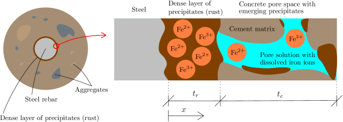
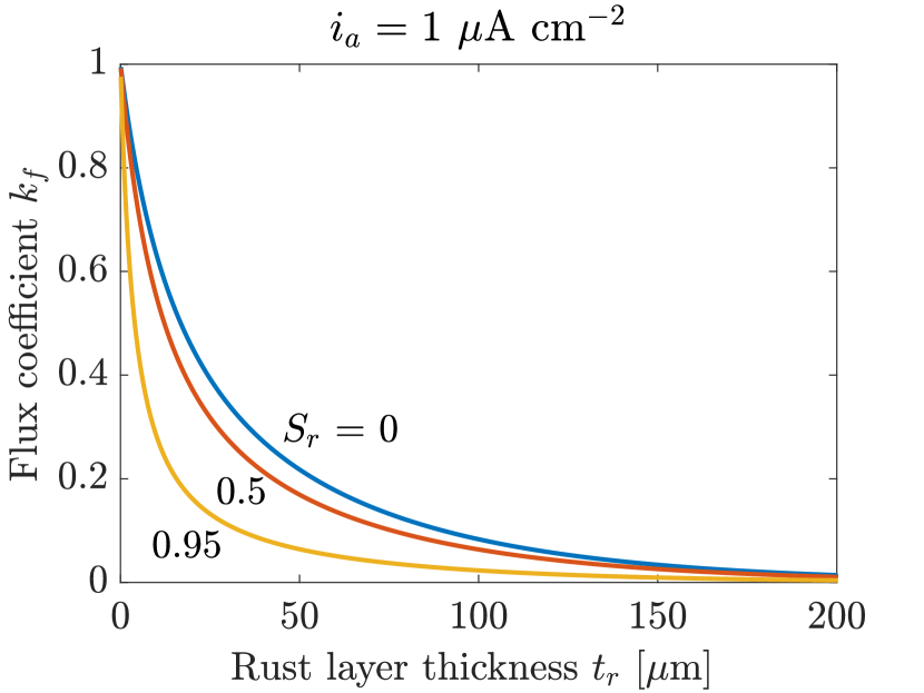
During corrosion, ferrous ions are released from the steel surface by electrochemical reaction (1a) and their flux follows Faraday’s law . A portion of the released ions and emerging ions precipitate to form a dense rust layer in the vicinity of the rebar while the remainder is transported further into the pore space to eventually precipitate there (see Fig. 5). The thickness of the rust layer is typically much smaller compared to the rebar radius. For this reason, the rust layer is not explicitly geometrically considered during domain discretization for numerical calculation, as this would strongly exacerbate the computational requirements. Instead, the steel domain is handled as unchanged in time, and the mechanical pressure of the accumulating dense rust layer on concrete is taken into consideration by additional pressure on the steel boundary, further discussed in Section 2.3. Thus, in reality, the flux of ferrous ions prescribed on the steel boundary is only the portion of this flux that did not precipitate into the dense rust layer. This flux reduction is mathematically incorporated by the flux reduction coefficient multiplying Faraday’s law-dictated flux .
To estimate , let us assume instantaneous precipitation of ferric ions and constant given liquid volume fraction , and let us simplify reactive transport equation (2) into its one-dimensional stationary form
| (7a) | ||||
| (7b) | ||||
Equation (7) is solved on an evolving domain , which is separated into the dense rust layer subdomain with diffusivity and the concrete subdomain with diffusivity , where changes in time (see Fig. 5). For the sake of simplicity, the thickness of the dense rust layer is considered to be equal to the thickness of the corroded steel layer predicted by Faraday’s law.
It is possible to solve equations (7a) and (7b) independently and analytically, considering Faraday’s law dictated flux at , at and a given unknown flux value at the current interface . From the assumption of flux continuity at , a solution for is obtained. If is further replaced by to consider the effect of pore-clogging with precipitates on diffusivity, the resulting flux can be expressed as
| (8) |
where the flux reduction coefficient
| (9) |
is calculated using rust-related and concrete-related constants
| (10) |
Based on the results of our previous study [29], it is set mm.
2.2 Phase-field description of precipitation-induced cracks
In this model, the phase-field cohesive zone model (PF-CZM) of Wu [34, 35] is employed, which allows for the calibration of the softening curve such that the quasi-brittle fracture nature of concrete is captured. Here a brief summary of the governing equations of the PF-CZM model and the necessary background is provided. For the derivation and more detailed explanation, see section 2.4 in Ref. [29]. The fracture problem is solved exclusively on the concrete domain while the steel in is assumed to remain linear elastic. The primary unknown variables in are the displacement vector
| (11) |
and the phase-field variable
| (12) |
where is the portion of concrete boundary with prescribed displacement . In (11) and (12), is the geometric dimension of the problem and function space is the Cartesian product of Sobolev spaces consisting of functions with square-integrable weak derivatives. The phase-field variable characterises the current damage of concrete such that for undamaged material and for a fully cracked material. Note that is not the traditional damage variable that directly reflects the relative change of stiffness, but it is linked to the material integrity through the degradation function, to be introduced later.
The small-strain tensor is used, and the total strain is additively decomposed into the elastic part and the precipitation eigenstrain . Because damage limits the stress that can be carried by the material, the Cauchy stress tensor is calculated as
| (13) |
where is the fourth-order isotropic elastic stiffness tensor of concrete, characterized by Young’s modulus and Poisson’s ratio , and is the degradation function that describes the remaining integrity of the material. Typically, it is a function that satisfies conditions and and is non-increasing and continuously differentiable in .
Assuming tractions prescribed on and a volume force acting on , the governing equations and the related boundary conditions for the coupled damage-displacement problem read
| (14a) | ||||
| (14b) | ||||
| (14c) | ||||
| (14d) | ||||
where is the fracture energy and is the characteristic phase-field length scale governing the size of the process zone [36]. To make the results independent of , it is recommended to use where is a characteristic length of the structure (e.g., the beam depth) and is the Irwin internal length, evaluated from the fracture energy, tensile strength and elongation modulus .
In the crack process zone, the characteristic size of the finite elements must be sufficiently small to provide good resolution of high strain gradients, typically 5-7 times smaller than [36]. In (14c) the crack driving force history function
| (15) |
is employed to secure the irreversibility of damage [37]. The function stores the maximum reached value of the crack driving force in time. Crack nucleation occurs when exceeds the damage nucleation threshold calculated from the basic properties of concrete. The function is the positive part of the maximum principal value of the effective stress tensor .
The softening curve resulting from the phase-field model is affected by the choice of the degradation function . For the PF-CZM model, Wu [34] proposed to use
| (16) |
This function is calibrated by an appropriate choice of parameters , , and , based on the required shape of the softening curve, characterized by the ratios
| (17) |
where is the crack opening at zero stress (full softening), is the initial slope of the softening curve (i.e., its negative slope at the onset of cracking), and
| (18) |
are the reference values that would correspond to linear softening.
For softening laws with zero stress attained at a finite value of crack opening, the parameter is set to 2, and for laws that approach zero stress only asymptotically, a value greater than 2 is appropriate. The other parameters of the degradation function (16) are then evaluated as
| (19) |
For concrete, the experimentally measured softening can usually be reasonably represented by the Hordijk-Cornelissen cohesive law [38], for which
| (20) |
and thus and . Wu [34] demonstrated that his version of the phase-field model indeed provides a close approximation of the Hordijk-Cornelissen curve if the parameters of the degradation function (16) are set to
| (21) | |||||
| (22) |
These are the values adopted in the present study. The parameter , linked to the choice of the characteristic length , will be evaluated from the first formula in Eq. (19).
2.3 Pressure of the accumulated rust layer
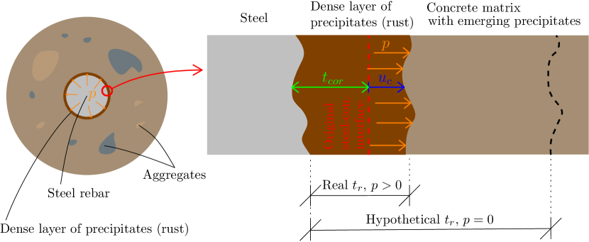
As was discussed in previous sections, and ions eventually precipitate into rust that either forms a dense rust layer in the vicinity of steel rebar or gradually fills the concrete pore space. Rust has a significantly lower density than original iron, typically by 3 - 6 times [39]. For this reason, if the volume characterised by thickness is vacated by the corrosion process, the dense rust layer would occupy 3 - 6 times larger volume under unconstrained conditions (see Fig. 6). However, the rust volumetric expansion is constrained by the concrete matrix and the expansion of the rust layer thus exerts pressure on the concrete boundary. Constrained rust volumetric expansion in the pore space also causes pressure on pore walls, which is described by the precipitation eigenstrain, as explained in the following section.
To estimate the pressure of a dense rust layer on concrete, let us virtually isolate the cylinder containing a rebar of radius and the adjacent layer of concrete with radius from the studied concrete specimen (see Fig. 1). Assuming the length of the cylinder , isotropic linear elasticity of concrete and symmetric boundary conditions, the thick-walled cylinder can be described as an axisymmetric linear elastic plane-strain problem. If the damage is simplified to be uniformly distributed across the cylinder, the displacement on the inner concrete boundary for a given pressure reads (the derivation is provided in A)
| (23) |
where is Poisson’s ratio of concrete. is the damaged secant modulus of concrete, calculated as the product of Young’s modulus of concrete and degradation function (see Section 2.2 for more details) evaluated on the inner concrete boundary. The concrete compliance constant thus encapsulates the impact of concrete sample geometry and material properties.
Both and in Eq. (23) are unknown, and thus it is necessary to link them by an additional equation. For this reason, let us now analyse the relation between pressure compressing the rust layer and the volume , which is (for small thicknesses) proportional to . Let us assume that the bulk modulus of rust is constant and equal to , with and being respectively the Young modulus and Poisson ratio of rust. The bulk modulus is the reciprocal value of the compressibility of rust, which is under isothermal conditions expressed as
| (24) |
Integration of (24) leads to
| (25) |
where is an integration constant, which has the meaning of the volume that would be occupied by the rust at zero pressure. By inversion, it is possible to express the pressure as
| (26) |
The rust layer of thickness occupies volume . The corrosion penetration is usually much smaller than the bar diameter. The assumption that leads to . Furthermore, the rust volume at zero pressure can be expressed as , where
| (27) |
is a volumetric expansion coefficient resulting from the disparity of molar volumes of steel and rust. This coefficient is evaluated from the mass fractions and of iron hydroxy-oxides and iron oxides in rust produced at the given corrosion current density (see Fig. 3) and the corresponding molar volume ratios and of oxide rust/iron and hydroxy-oxide rust/iron, respectively. Substituting the expressions for and into Eq. (26) results in
| (28) |
Using the previously derived relation (23), it is easy to eliminate the unknown pressure from Eq. (28) and construct an equation for a single unknown, :
| (29) |
This can be rewritten in the simple form
| (30) |
in which is a known right-hand side and the left-hand side is a nonlinear function of unknown . For , Eq. (30) has a unique real solution , where is the so-called Lambert function, also known as the product logarithm. Since is always positive for our problem, the solution of Eq. (29) can be written as
| (31) |
The corresponding pressure is easily expressed as .
Let us note that even though the formula (31) has been derived assuming axial symmetry, the real distribution of damage is not uniform on the boundary between steel and concrete due to the gradual localisation of cracks. For this reason, the assumption of axisymmetry will be violated and the formula will be evaluated point-wise on the steel-concrete boundary.
2.4 Precipitation eigenstrain
and ions transported into the pore space gradually precipitate there into iron oxides and hydroxy-oxides. As was the case for the dense rust layer adjacent to the rebar, rust accumulates in the confined conditions of concrete pore space and exerts pressure on concrete pore walls [39, 3] (see Fig. 2 for a graphical illustration). This statement is supported both by the similarity with the well-described damage mechanism of precipitating salts in porous materials [40, 41, 42, 43, 44, 45, 46] and the recent simulations of Korec et al. [29], which revealed that this mechanism could considerably contribute to corrosion-induced fracture in its early stages until the pore space surrounding rebar is locally filled. Macroscopic stress resulting from the accumulation of rust in the pore space under confined conditions is simulated with the precipitation eigenstrain proposed by Korec et al. [29], based on the previous works of Coussy [43], Krajcinovic et al. [47] and Mura [48]. The precipitation eigenstrain is calculated as
| (32) |
where is the bulk modulus of rust-filled concrete calculated from Young’s modulus of rust-filled concrete and concrete Poisson ratio . Because the mechanical properties of rust and concrete are very different, is interpolated between Young’s modulus of rust-free concrete and rust Young modulus following the rule of mixtures.
2.5 Damage–dependent diffusivity tensor
Dissolved and ions are transported much more easily through emerging cracks than through the surrounding concrete matrix. For this reason, the damage-dependent diffusivity tensor [29, 49] is considered, and defined as
| (33) |
where is the diffusivity of the considered species in concrete and controls the diffusivity of the cracked material.
2.6 Overview of the governing equations
The solved coupled problem comprises six differential equations (34a)–(34f) for six unknown variables – displacement vector , phase-field variable , ions concentration , ions concentration , hydroxy-oxide rust volume fraction and oxide rust volume fraction :
| (34a) | ||||
| (34b) | ||||
| (34c) | ||||
| (34d) | ||||
| (34e) | ||||
| (34f) | ||||
| Differential equations (34a)–(34d) are associated (in the presented order) with boundary conditions | ||||
| (35a) | ||||
| (35b) | ||||
| (35c) | ||||
| (35d) | ||||
Boundary conditions for equations (34e) and (34f) are not required because these equations do not contain any spatial derivatives.
The resulting coupled system of differential equations is numerically solved with the finite element method using COMSOL Multiphysics software. The domain is discretised with linear triangular elements and a staggered solution scheme is employed. To achieve mesh-independent results, mm is chosen such that would be five times larger than the maximum element size [36].
3 Results
After the presentation of parameter values employed for numerical simulations (Section 3.1), the observed characteristic features of the model are discussed in Section 3.2, together with the implications for the understanding of corrosion-induced cracking. Then, in Section 3.3, impressed current tests with varying corrosion current density from the comprehensive experimental study of Pedrosa and Andrade [11] are simulated. The predicted relations between the surface crack and the thickness of the corroded steel layer are fitted with linear functions and their slopes are compared with the experimental measurements, revealing the ability of the model to capture the decrease of the slope with increasing corrosion current density. Based on the obtained results, a correction factor to be applied on the crack width slope obtained from accelerated impressed current tests is proposed, allowing for extrapolation of results to naturally corroding structures.
3.1 Choice of model parameters
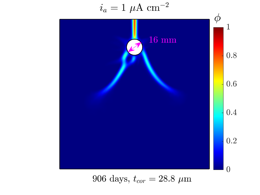
The mechanical parameters listed in Table LABEL:tab:tableMechRust1 correspond to the concrete specimens employed in the comprehensive experimental study by Pedrosa and Andrade [11], in which the corrosion-induced cracking under different values of applied corrosion current density was analysed. The 15 x 15 x 50 cm samples reinforced with a 16 mm rebar were separated into two groups with curing times of 28 and 147 days, which led to different mechanical properties. Pedrosa and Andrade [11] measured the tensile and compressive strength. The fracture energy is estimated using the formula of Bažant and Becq-Giraudon [50]. For the steel rebar, Young’s modulus of 205 GPa and Poisson’s ratio of 0.28 are assumed, as these are common values for steel.
| Properties of concrete - 28 and 147 days cured samples | |||
| Parameter | Value | Unit | Source |
| Compressive strength | 37.5 & 54.7 | MPa | [11] |
| Tensile strength | 2.2 & 3.9 | MPa | [11] |
| Young’s modulus | 33 & 36 | GPa | [51] |
| Poisson’s ratio | 0.2 & 0.2 | - | [51] |
| Fracture energy | 95 & 114 | N m-1 | [50] |
Only the capillary porosity of cement paste is considered to be relevant in the vicinity of rebar, and it is estimated using the model of Powers and Brownyard [52], assuming the degree of hydration of 0.9. The values of the initial diffusivity of ions and ions in concrete are adopted from the study of Stefanoni et al. [31], where they were estimated from the known diffusivity in solution assuming that the ratio between the diffusivity in water and concrete is the same as for chloride ions. The diffusivity of iron ions in cracks was considered identical to the diffusivity in the pore solution.
| Parameter | Value | Unit | Source |
| Properties of rust | |||
| Young’s modulus | MPa | [27] | |
| Poisson’s ratio | - | [27] | |
| Molar volume ratio of iron oxide rust to iron | - | [27, 12, 17] | |
| Molar volume ratio of iron hydroxy-oxide rust to iron | - | [27, 12, 17] | |
| Diffusivity of iron ions in rust | m2 s-1 | [53] | |
| Transport properties of concrete | |||
| Capillary porosity | - | [52] | |
| Initial concrete diffusivity and | m2 s-1 | [31] | |
| Cracked concrete diffusivity and | m2 s-1 | [31, 32] | |
Molar volume ratios of iron oxide rust/iron and hydroxy-oxide rust/iron characterising rust volumetric expansion are chosen in the range of values reported by Zhao and Jin [27], Vu et al. [12] and Zhang et al. [17] for commonly present iron oxides and iron hydroxy-oxides. The measurements of Young’s modulus and Poisson’s ratio of rust are infamously scattered in the current literature, so two intermediate values within the range reported by Zhao and Jin [27] are considered; they were identified to lead to an accurate prediction of crack width in the previous study of the authors [29]. The diffusivity for iron ions in rust was adopted from the study of Ansari et al. [53].
Let us also stress that in numerical simulations conducted within this study, uniform corrosion and thus the constant value of corrosion current density are considered. This is because impressed current tests typically ensure uniform corrosion by artificially introducing high chloride concentration into concrete, as was done in tests by Pedrosa and Andrade [11] considered in this study. For the results on the simulation of a non-uniform chloride-induced corrosion under natural conditions with a similar model as in this study, see Ref. [54].
3.2 General aspects of the model (the impact of the dense rust layer)
In the proposed model, rust precipitates either in the dense rust layer adjacent to the corroding rebar surface or deeper in the pore space of concrete. The flux of ions released from the corroding steel surface according to Faraday’s law is divided between these two processes based on the flux reduction coefficient . As can be seen in Fig. 8(a), if there is no dense rust layer and all released ferrous ions are transported into the concrete pore space. With the advance of the corrosion process, the thickness of the dense rust layer increases, decreasing the portion of ion flux that is released to the concrete pore space. For a thick rust layer, eventually vanishes, leaving all released ions to contribute to the build-up of the dense rust layer. Also, as saturation of the pore space with precipitates increases, the ion diffusivity in concrete is reduced, which decreases the ability of ions to escape the dense rust layer.
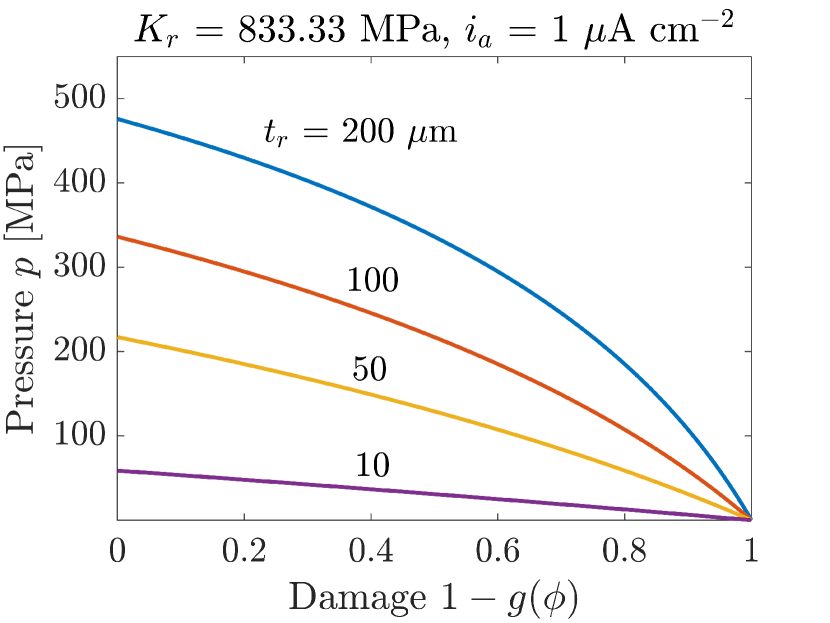
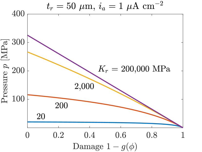
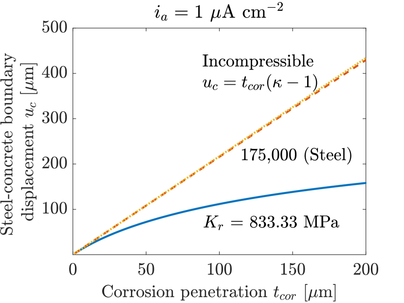
The accumulation of precipitated rust in (A) a dense layer of corrosion products in the space vacated by steel corrosion, and (B) the concrete pore space under constrained conditions, induces pressure on the concrete matrix. Pressure in the dense rust layer increases with its thickness (see Figs. 7(a) and 7(c)). However, it also non-linearly decreases with damage, since concrete becomes more compliant and the expansion of rust is then less constrained (Figs. 7(a) and 7(b)). The mechanical properties of rust have a strong influence on (see the dependence on the bulk modulus of rust in Fig. 7(b)). If the bulk modulus of rust was similar to steel, pressure would decrease almost in proportion to the degradation factor . However, for lower bulk moduli of rust, in tens or hundreds of MPa, the decrease deviates from linearity and the induced pressure is significantly smaller. Many currently available models neglect the impact of rust compressibility and simplify the steel-concrete boundary displacement to be as if rust was incompressible. As demonstrated in Fig. 7(c), this assumption leads to a nearly equivalent displacement prediction as if rust elastic properties were equivalent to those of steel. Since the experimental measurement of Young’s modulus and Poisson’s ratio of rust are quite scattered [27] in the range from 100 MPa to 360 GPa, our results stress the need for accurate characterization studies.
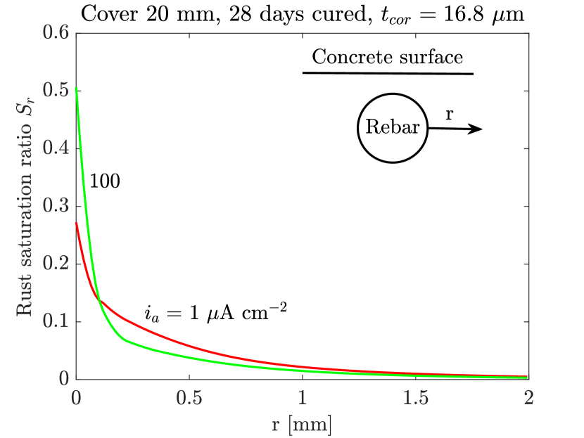
From the conducted simulations, it was observed that the distribution of rust in pore space differed for natural-like low corrosion current densities (about 1 \unit\micro\per\centi^2 and lower) compared to high current densities (tens or hundreds of \unit\micro\per\centi^2) typical for corrosion induced by accelerated impressed current (see Fig. 8(b)). In the case of high current densities, the rust was distributed closer to the steel surface than for low current densities, which led to a significantly higher rust saturation of pores in the vicinity of steel rebar. Thus, pores are blocked with rust earlier than in natural conditions, not allowing for additional transport of dissolved iron species into pore space. This suggests that during the natural corrosion process, significantly more dissolved iron species can escape to the concrete pore space and precipitate there. The rapid increase of the rust saturation for high current densities probably results from significantly higher concentrations of released ions, which accelerates the precipitation reactions (1c) and (1d). Similar results were obtained in the computational study of Stefanoni et al. [31].
3.3 The impact of the magnitude of applied corrosion current density on crack width—analysis and validation
Fig. 9(c) shows the geometry and the typical fracture pattern observed for the simulated impressed current tests. The main crack propagates across the shortest distance between the concrete surface and the steel rebar, perpendicularly to the concrete surface, and opens wide with the ongoing corrosion process. In addition, two other lateral cracks develop. The surface crack width
| (36) |
is calculated as the integral of the -component (i.e., the normal component in the direction perpendicular to the crack) of the inelastic strain tensor over the upper concrete surface [55]. The inelastic strain is obtained by subtracting the eigenstrain and the elastic strain from the total strain. For the same thickness of corroded steel layer , the crack width decreases with increasing applied corrosion current density. This trend agrees with the experimental observations of [10, 11, 16, 12, 56, 15, 14] and is the result of the hypothesis that the chemical composition of rust, in particular the mass ratio of iron oxides and iron hydroxy-oxides, changes with the magnitude of the applied current density (see Fig. 3) such that the rust density increases with increasing current density, reducing the pressure caused by constrained expansion.
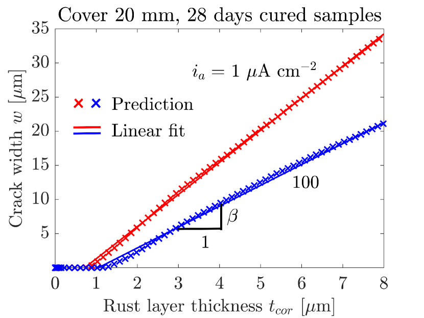
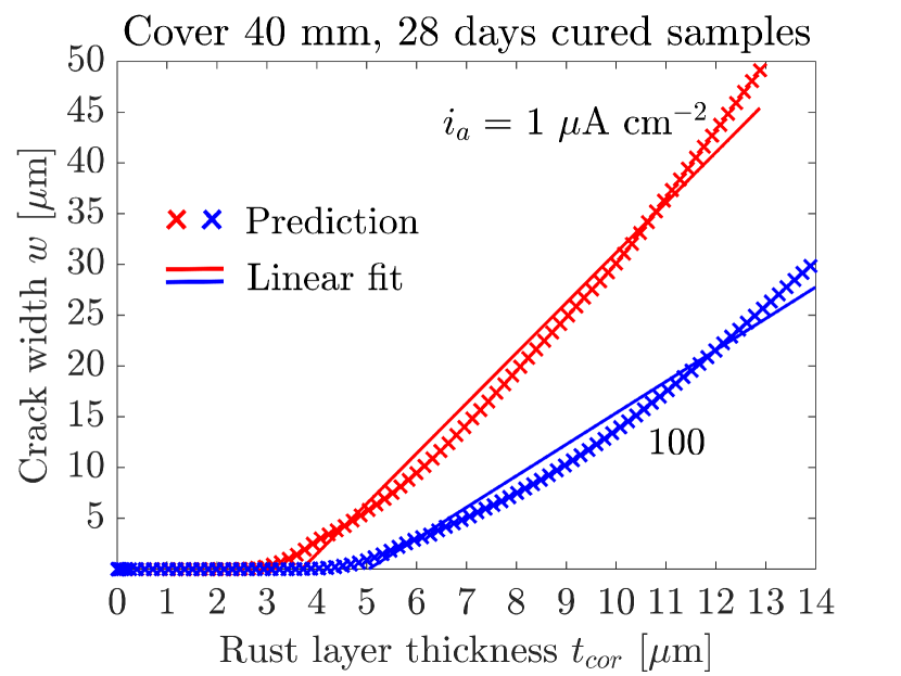
The predicted crack width is linearly fitted by , so that the crack width slope can be compared with its experimental counterpart measured by Pedrosa and Andrade [11], who employed the same fitting procedure on their experimentally measured crack widths. To prevent the distortion caused by nonlinearity for zero and very small crack widths, only \unit\micro was considered for fitting. Though linear fitting approximates the results very accurately for the thinner concrete of 20 mm (Fig. 9(a)), the crack width increases superlinearly with for the thicker cover of 40 mm, which hinders the accuracy of the linear fitting procedure. For thicker concrete covers, the predicted crack width slope is thus affected by the maximum evaluated and linear fitting is not optimal. In the discussed simulations, the maximal was 8 \unit\micro and 12 \unit\micro for the cases of 20 and 40 mm thick concrete cover, respectively.
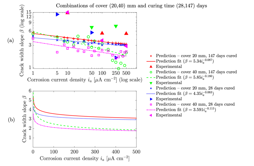
The comparison of the predicted crack width slope with the results recovered from the fitting of experimental measurements [11] reveals that the predicted data lie in the experimental range and that the trend characterised by the decay with a negative power of current density [11] is reproduced very well. For a better understanding of how well the various sets of predicted data agree with this trend, the predicted results are fitted with , where \unit\micro\per\centi^2 is the reference corrosion current density. In Fig. LABEL:CrWidSlope, an excellent agreement with the data for the smaller concrete cover of 20 mm can be observed. On the other hand, the predictions for the thicker concrete cover of 40 mm are significantly more scattered, even though the overall trend still agrees. Fig. 9(a) and Fig. 9(b) suggest that the accuracy of the predictions is clearly related to how well can the data be fitted with a linear function. While data for the 20 mm cover are fitted very well, the non-linear dependency for the thicker 40 mm cover diminishes the representative value of . Also, it was observed that with the increasing thickness of the concrete cover, the model becomes numerically more sensitive such that there are several similar crack patterns that lead to a slightly different evolution of the surface crack width. The realization of a particular crack pattern appears to be triggered by small numerical differences.
Critically, the proposed model captures the initially rapid decrease of with increasing current density suggested by the experimental data of Pedrosa and Andrade [11]. For current densities larger than approximately 50 \unit\micro\per\centi^2, the decrease of is more moderate. As can be seen in Fig. LABEL:CrWidSlope, this agrees qualitatively very well with the experiments. However, the magnitude of slopes observed by Pedrosa and Andrade [11] for current densities smaller than 10 \unit\micro\per\centi^2 were even several times larger than those recovered from numerical simulations. Though the paper of Pedrosa and Andrade [11] is currently the most comprehensive experimental study on the impact of the magnitude of impressed current on the crack width slope, the total number of tested specimen was arguably small (11 in total and every test was conducted only once which does not allow to evaluate experimental error). Thus, it is not clear whether the observed discrepancy between the quantitative values of numerical predictions and experiments can be attributed to the experimental error or some other phenomena unaccounted by the model. Clearly, more comprehensive experimental campaigns are needed. For current densities larger than 10 \unit\micro\per\centi^2, numerical predictions agree quantitatively better with experimental measurements, though they mostly underestimate the experimental values.
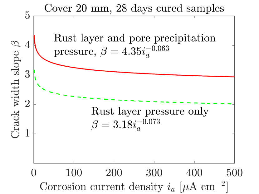
The comparison of data for the four combinations of two curing times (leading to different mechanical properties) and two concrete covers in Fig. LABEL:CrWidSlope indicate that increases with increasing curing time (i.e. enhanced mechanical properties). Also, a larger cover can lead to larger for small natural-like current densities (within the evaluated case studies, this held for the combination of 40 mm cover and 147 days curing time), as was previously observed in Ref. [29]. The modelling results in Fig. LABEL:CrWidSlope indicate that the influence of concrete cover is significantly more important than of curing time (i.e. concrete strength). Also, it appears that the larger the current density, the smaller the impact of curing time (i.e. concrete strength) on the crack width slope. The pressure generated by the constrained accumulation of the dense rust layer has a considerable impact on corrosion-induced fracture (see Fig 11(a)), although the role of the pressure of rust precipitating in the pore space of concrete is also not negligible. However, one has to bear in mind that the proposed model overestimates the corrosion-induced pressure of the dense rust layer, as the entire volume of steel vacated by corrosion is assumed to be filled with rust regardless of the portion of ferrous ions escaping into pore space. In reality, the pressure of the dense rust layer can be reasonably expected to be smaller, raising the relative impact of the pressure of precipitates accumulating in the pore space.
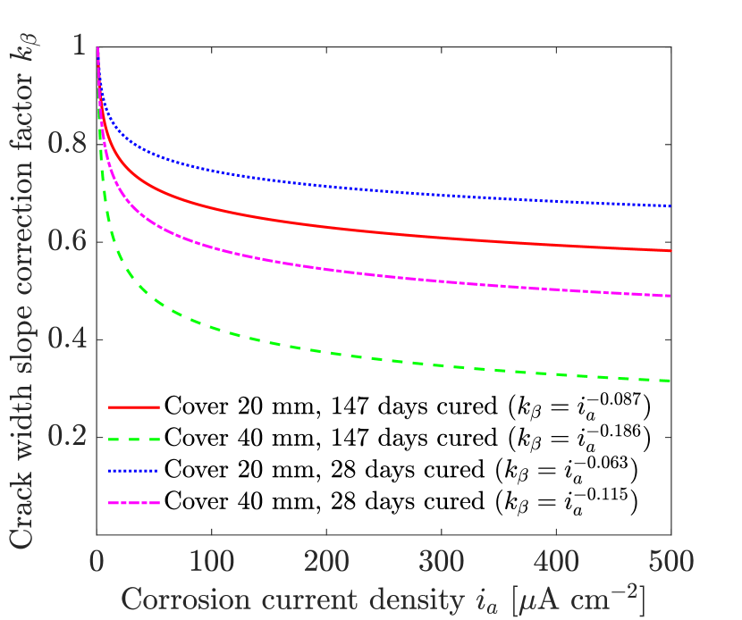
In Fig. 11(b), the relative error of slope , caused by the acceleration of the applied current compared to corrosion in natural conditions, is evaluated in terms of newly proposed crack width slope correction factor inspired by the loading correction factor of Vu et al. [12] for time-to-cracking. The correction factor was calculated as . The factor can thus be interpreted as the relative error caused by the acceleration of the impressed current tests compared to results that could be expected in natural conditions when \unit\micro\per\centi^2. One can see that the error induced by current acceleration strongly increases with the thickness of the concrete cover. While for 147 days cured samples and \unit\micro\per\centi^2, for the 20 mm thick cover, it drops to for a 40 mm thick cover. The same trend was experimentally documented by Alonso et al. [10] who reported even six times larger if current density was accelerated from 10 to 100 \unit\micro\per\centi^2 for the concrete cover of 70 mm. Also, it can be observed that the impact of curing time on is smaller than the impact of the thickness of the concrete cover.
 (a)
(a)
 (b)
(b)
The knowledge of the accurate slope of crack width with respect to corrosion penetration in natural conditions is important for the accurate predictions of the length of the corrosion propagation period (time since corrosion initiation to critical corrosion-induced delamination/spalling of concrete cover). Currently, durability estimates in national design codes are based on time until corrosion initiation, which is dictated by the time needed for the diffusion of aggressive species such as chlorides from exposed concrete surfaces through concrete cover to steel rebars. This approach is overly conservative, as even though corrosion initiation is usually the longest part of the corrosion process, the length of the propagation period can be substantial. For example, the results for a 40 mm thick concrete cover and concrete cured for 28 days indicate that under natural conditions (typically \unit\micro\per\centi^2) the propagation period would last for at least 7 years until the surface crack width of 0.3 mm (a commonly used Eurocode criterion of limit serviceability state) was reached. That said, even the crack opening of 0.3 mm can underestimate the time when serious delamination/spalling occurs [10, 57].
4 Conclusions
A phase-field-based model for corrosion-induced cracking of reinforced concrete specimens subjected to uniform corrosion was presented. Based on the experimental findings (Ref. [17]), the hypothesis that the chemical composition of rust characterized by the mass ratio of its main components (iron oxides and iron hydroxy-oxides) changes with the applied corrosion current density was tested. This affects the density of rust, which increases with increasing current density, thereby reducing the corrosion-induced pressure in the process. The main findings can be summarised as follows:
-
1.
The simulation results strongly support the hypothesis of changing chemical composition of rust with the applied corrosion current density as the explanation of the experimentally observed slower crack growth (with respect to corrosion penetration) in accelerated impressed current tests compared to corrosion in natural conditions [10, 11, 16, 12, 56, 15, 14, 12], which has been debated for nearly three decades.
-
2.
Simulations support the experimentally recovered conclusion of Pedrosa and Andrade [11] that the decay of the slope of the crack width as a function of corrosion penetration is proportional to a negative power of corrosion current density, especially for thinner concrete covers.
-
3.
The non-linearity of the crack width dependence on corrosion penetration increases with the thickness of the concrete cover.
-
4.
The relative error in the estimate of crack width slope compared to corrosion in natural conditions increases with the applied corrosion current density and the thickness of the concrete cover.
-
5.
Current design codes base the corrosion durability estimates of concrete structures on time for corrosion initiation (i.e. the transport of aggressive species such as chlorides through concrete cover). However, this approach is overly conservative and the consideration of the corrosion propagation stage of corrosion (since corrosion initiation to serious delamination/spalling) in the structure’s service life can prolong the durability estimates for years. For a 40 mm thick concrete cover and concrete cured for 28 days, the proposed model predicts that under natural conditions ( \unit\micro\per\centi^2) at least 7 years would pass until the surface crack width of 0.3 mm is reached.
A newly proposed crack width slope correction factor can be calculated from the proposed model and allows for the estimate of the relative error caused by the acceleration of the impressed current test to a specified value of corrosion current density. With this, the current density can be picked such that the error in the slope of crack width as a function of corrosion penetration remains (e.g.) below 10. In general, the proposed modelling framework allows for computational impressed current testing as the support of experimental efforts.
5 Acknowledgements
The authors would like to express their gratitude to Prof Carmen Andrade (CIMNE International Center for Numerical Methods in Engineering, Barcelona) for her invaluable advice and stimulating discussions. E. Korec acknowledges financial support from the Imperial College President’s PhD Scholarships. M. Jirásek acknowledges previous financial support of the European Regional Development Fund (Center of Advanced Applied Sciences, project CZ.02.1.01/0.0/0.0/16_19/0000778). E. Martínez-Pañeda was supported by an UKRI Future Leaders Fellowship [grant MR/V024124/1]. We additionally acknowledge computational resources and support provided by the Imperial College Research Computing Service (http://doi.org/10.14469/hpc/2232).
Appendix A Axisymmetric thick-walled concrete cylinder problem
To calculate the pressure of the dense rust layer in Section 2.3, the concrete layer adjacent to the steel rebar is virtually isolated from the considered sample as a two-dimensional thick-walled cylinder with inner radius (equal to the rebar radius) and outer radius (see Fig. 1).
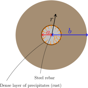
Because the length of the cylinder is typically much larger than and material homogeneity and symmetric boundary conditions are assumed, the thick-walled cylinder can be mechanically described as an axisymmetric plane-strain problem. The plane is described by two polar coordinates—polar angle and radius . The equilibrium equations for in-plane stress components read
| (37) | ||||
and the material behaviour is characterized by Hooke’s law for plane strain,
| (38) | ||||
in which the strains are linked to the displacements by
| (39) | ||||
The assumption of axial symmetry makes all considered quantities independent of , and also leads to . Therefore, from (39) follows that and (38) yields . Equilibrium equations (37) and strain-displacement equations (39) are simplified to
| (40) |
| (41) | ||||
If (41) is substituted into (38) and the resulting relations into (40), an ordinary differential equation is obtained
| (42) |
The general solution of this equation reads
| (43) |
where and are unknown real constants, to be calculated from boundary conditions. The corresponding strains and stresses are
| (44) | |||||
| (45) | |||||
| (46) | |||||
| (47) |
Under uniform corrosion, the constrained volumetric expansion of the dense rust layer leads to pressure on the inner surface of the thick-walled cylinder, which generates compressive stress . It is supposed that the outer boundary of the concrete cylinder is stress-free, i.e., . Substituting these boundary conditions into (46), two equations for the integration constants are obtained, from which
| (48) | |||||
| (49) |
The displacement at the inner boundary induced by pressure is then given by
| (50) |
Introducing a dimensionless shape factor , the compliance is expressed as
| (51) |
and write the relation between pressure and displacement at the inner boundary in the form
| (52) |
The derivation has been done for concrete considered as an elastic material characterized by Young’s modulus and Poisson’s ratio . If the concrete is damaged, should be replaced by the secant modulus where is the degradation function and is the phase-field variable that describes the state of damage. In general, varies in the radial as well as circumferential direction, and the problem is no longer axially symmetric and does not have an analytical solution. For simplicity, the effect of damage is considered only approximately by using a uniformly reduced modulus , where the degradation function is evaluated on the inner concrete boundary, i.e., at . This means that the damage of concrete is simplified to be uniformly distributed over the thick-walled cylinder and the value of the damage is the same as on the inner concrete boundary. The final formula for the compliance factor to be used in (52) is then
| (53) |
References
- Gehlen et al. [2011] C. Gehlen, C. Andrade, M. Bartholomew, J. Cairns, J. Gulikers, F. Javier Leon, S. Matthews, P. McKenna, K. Osterminski, A. Paeglitis, D. Straub, Fib Bulletin 59 - Condition control and assessment of reinforced concrete structures exposed to corrosive environments (carbonation/chlorides), fib - The International Federation for Structural Concrete, 2011.
- Jones and Marsh [1997] A. E. K. Jones, B. K. Marsh, Development of an holistic approach to ensure the durability of new concrete construction, British Cement Association (BCA), 1997.
- Angst [2018] U. M. Angst, Challenges and opportunities in corrosion of steel in concrete, Materials and Structures 51 (2018) 1–20.
- Yuan et al. [2007] Y. Yuan, Y. Ji, S. P. Shah, Comparison of two accelerated corrosion techniques for concrete structures, ACI Structural Journal 104 (2007) 344–347.
- Otieno et al. [2012] M. Otieno, H. Beushausen, M. Alexander, Prediction of corrosion rate in reinforced concrete structures - A critical review and preliminary results, Materials and Corrosion 63 (2012) 777–790.
- Otieno et al. [2016] M. Otieno, H. Beushausen, M. Alexander, Chloride-induced corrosion of steel in cracked concrete - Part I: Experimental studies under accelerated and natural marine environments, Cement and Concrete Research 79 (2016) 373–385.
- Andrade [2023] C. Andrade, Steel corrosion rates in concrete in contact to sea water, Cement and Concrete Research 165 (2023) 107085.
- Walsh and Sagüés [2016] M. T. Walsh, A. A. Sagüés, Steel corrosion in submerged concrete structures-part 1: Field observations and corrosion distribution modeling, Corrosion 72 (2016) 518–533.
- Andrade [2023] C. Andrade, Role of Oxygen and Humidity in the Reinforcement Corrosion, in: Proceedings of the 75th RILEM Annual Week 2021: Advances in Sustainable Construction Materials and Structures, Springer, Cham, Switzerland, 2023, pp. 316–325.
- Alonso et al. [1996] C. Alonso, C. Andrade, J. Rodriguez, J. M. Diez, Factors controlling cracking of concrete affected by reinforcement corrosion, Materials and Structures 31 (1996) 435–441.
- Pedrosa and Andrade [2017] F. Pedrosa, C. Andrade, Corrosion induced cracking: Effect of different corrosion rates on crack width evolution, Construction and Building Materials 133 (2017) 525–533.
- Vu et al. [2005] K. Vu, M. G. Stewart, J. Mullard, Corrosion-induced cracking: Experimental data and predictive models, ACI Structural Journal 102 (2005) 719–726.
- Saifullah and Clark [1994] M. Saifullah, L. A. Clark, Effect of corrosion rate on the bond strength of corroded reinforcement, Corrosion and corrosion protection of steel in concrete 1 (1994) 591–602.
- Mullard and Stewart [2011] J. A. Mullard, M. G. Stewart, Corrosion-induced cover cracking: New test data and predictive models, ACI Structural Journal 108 (2011) 71–79.
- El Maaddawy and Soudki [2003] T. A. El Maaddawy, K. A. Soudki, Effectiveness of Impressed Current Technique to Simulate Corrosion of Steel Reinforcement in Concrete, Journal of Materials in Civil Engineering 15 (2003) 41–47.
- Mangat and Elgarf [1999] P. S. Mangat, M. S. Elgarf, Strength and serviceability of repaired reinforced concrete beams undergoing reinforcement corrosion, Magazine of Concrete Research 51 (1999) 97–112.
- Zhang et al. [2019] W. Zhang, J. Chen, X. Luo, Effects of impressed current density on corrosion induced cracking of concrete cover, Construction and Building Materials 204 (2019) 213–223.
- Liu et al. [2020] Q. Liu, R. K. L. Su, C. Q. Li, K. Shih, C. Liao, In-situ deformation modulus of rust in concrete under different levels of confinement and rates of corrosion, Construction and Building Materials 255 (2020) 119369.
- Chitty et al. [2005] W. J. Chitty, P. Dillmann, V. L’Hostis, C. Lombard, Long-term corrosion resistance of metallic reinforcements in concrete - A study of corrosion mechanisms based on archaeological artefacts, Corrosion Science 47 (2005) 1555–1581.
- Köliö et al. [2015] A. Köliö, M. Honkanen, J. Lahdensivu, M. Vippola, M. Pentti, Corrosion products of carbonation induced corrosion in existing reinforced concrete facades, Cement and Concrete Research 78 (2015) 200–207.
- Zhang et al. [2017] X. Zhang, M. Li, L. Tang, S. A. Memon, G. Ma, F. Xing, H. Sun, Corrosion induced stress field and cracking time of reinforced concrete with initial defects: Analytical modeling and experimental investigation, Corrosion Science 120 (2017) 158–170.
- Caré et al. [2008] S. Caré, Q. T. Nguyen, V. L’Hostis, Y. Berthaud, Mechanical properties of the rust layer induced by impressed current method in reinforced mortar, Cement and Concrete Research 38 (2008) 1079–1091.
- Wong et al. [2010] H. S. Wong, Y. X. Zhao, A. R. Karimi, N. R. Buenfeld, W. L. Jin, On the penetration of corrosion products from reinforcing steel into concrete due to chloride-induced corrosion, Corrosion Science 52 (2010) 2469–2480.
- Zhao et al. [2011] Y. Zhao, H. Ren, H. Dai, W. Jin, Composition and expansion coefficient of rust based on X-ray diffraction and thermal analysis, Corrosion Science 53 (2011) 1646–1658.
- Furcas et al. [2022] F. E. Furcas, B. Lothenbach, O. B. Isgor, S. Mundra, Z. Zhang, U. M. Angst, Solubility and speciation of iron in cementitious systems, Cement and Concrete Research 151 (2022) 106620.
- Wieland et al. [2023] E. Wieland, G. D. Miron, B. Ma, G. Geng, B. Lothenbach, Speciation of iron(II/III) at the iron-cement interface: a review, Materials and Structures 56 (2023) 1–24.
- Zhao and Jin [2016] Y. Zhao, W. Jin, Chapter 2 - Steel Corrosion in Concrete, in: Y. Zhao, W. Jin (Eds.), Steel Corrosion-Induced Concrete Cracking, Butterworth-Heinemann, 2016, pp. 19–29.
- Sola et al. [2019] E. Sola, J. Ožbolt, G. Balabanić, Z. M. Mir, Experimental and numerical study of accelerated corrosion of steel reinforcement in concrete: Transport of corrosion products, Cement and Concrete Research 120 (2019) 119–131.
- Korec et al. [2023] E. Korec, M. Jirásek, H. S. Wong, E. Martínez-Pañeda, A phase-field chemo-mechanical model for corrosion-induced cracking in reinforced concrete, Construction and Building Materials 393 (2023) 131964.
- Marchand et al. [2016] J. Marchand, E. Samson, K. A. Snyder, J. J. Beaudoin, Unsaturated Porous Media: Ion Transport Mechanism Modeling, in: Encyclopedia of Surface and Colloid Science, Third Edition, CRC Press, 2016, pp. 7488–7497.
- Stefanoni et al. [2018] M. Stefanoni, Z. Zhang, U. M. Angst, B. Elsener, The kinetic competition between transport and oxidation of ferrous ions governs precipitation of corrosion products in carbonated concrete, RILEM Technical Letters 3 (2018) 8–16.
- Leupin et al. [2021] O. X. Leupin, N. R. Smart, Z. Zhang, M. Stefanoni, U. M. Angst, A. Papafotiou, N. Diomidis, Anaerobic corrosion of carbon steel in bentonite: An evolving interface, Corrosion Science 187 (2021) 109523.
- Zhang and Angst [2021] Z. Zhang, U. M. Angst, Modelling transport and precipitation of corrosion products in cementitious materials: A sensitivity analysis, in: Life-Cycle Civil Engineering: Innovation, Theory and Practice, February, 2021, pp. 747–753.
- Wu [2017] J.-Y. Wu, A unified phase-field theory for the mechanics of damage and quasi-brittle failure, Journal of the Mechanics and Physics of Solids 103 (2017) 72–99.
- Wu [2018] J.-Y. Wu, Robust numerical implementation of non-standard phase-field damage models for failure in solids, Computer Methods in Applied Mechanics and Engineering 340 (2018) 767–797.
- Kristensen et al. [2021] P. K. Kristensen, C. F. Niordson, E. Martínez-Pañeda, An assessment of phase field fracture: Crack initiation and growth, Philosophical Transactions of the Royal Society A: Mathematical, Physical and Engineering Sciences 379 (2021) 20210021.
- Miehe et al. [2015] C. Miehe, L. M. Schänzel, H. Ulmer, Phase field modeling of fracture in multi-physics problems. Part I. Balance of crack surface and failure criteria for brittle crack propagation in thermo-elastic solids, Computer Methods in Applied Mechanics and Engineering 294 (2015) 449–485.
- Cornelissen et al. [1962] H. A. W. Cornelissen, D. A. Hordijk, H. W. Reinhardt, Two-Dimensional Theories of Anchorage Zone Stresses in Post-Tensioned Prestressed Beams, ACI Journal Proceedings 59 (1962) 45–56.
- Angst [2019] U. M. Angst, Durable concrete structures: cracks & corrosion and corrosion & cracks, in: P. G. G. Pijaudier-Cabot, C. L. Borderie (Eds.), 10th International Conference on Fracture Mechanics of Concrete and Concrete Structures FraMCoS-X, 2019, p. 233307.
- Scherer [1999] G. W. Scherer, Crystallization in pores, Cement and Concrete Research 29 (1999) 1347–1358.
- Flatt et al. [2014] R. J. Flatt, F. Caruso, A. M. A. Sanchez, G. W. Scherer, Chemo-mechanics of salt damage in stone, Nature Communications 5 (2014) 1–5.
- Flatt et al. [2017] R. J. Flatt, N. Aly Mohamed, F. Caruso, H. Derluyn, J. Desarnaud, B. Lubelli, R. M. Espinosa, L. Pel, C. Rodriguez-Navarro, G. W. Scherer, N. Shahidzadeh, M. Steiger, Predicting salt damage in practice: A theoretical insight into laboratory tests., RILEM Technical Letters 2 (2017) 108–118.
- Coussy [2006] O. Coussy, Deformation and stress from in-pore drying-induced crystallization of salt, Journal of the Mechanics and Physics of Solids 54 (2006) 1517–1547.
- Castellazzi et al. [2013] G. Castellazzi, C. Colla, S. De Miranda, G. Formica, E. Gabrielli, L. Molari, F. Ubertini, A coupled multiphase model for hygrothermal analysis of masonry structures and prediction of stress induced by salt crystallization, Construction and Building Materials 41 (2013) 717–731.
- Koniorczyk and Gawin [2012] M. Koniorczyk, D. Gawin, Modelling of salt crystallization in building materials with microstructure - Poromechanical approach, Construction and Building Materials 36 (2012) 860–873.
- Espinosa et al. [2008] R. M. Espinosa, L. Franke, G. Deckelmann, Phase changes of salts in porous materials: Crystallization, hydration and deliquescence, Construction and Building Materials 22 (2008) 1758–1773.
- Krajcinovic et al. [1992] D. Krajcinovic, M. Basista, K. Mallick, D. Sumarac, Chemo-micromechanics of brittle solids, Journal of the Mechanics and Physics of Solids 40 (1992) 965–990.
- Mura [1987] T. Mura, Micromechanics of defects in solids, Springer Netherlands, 1987.
- Wu and De Lorenzis [2016] T. Wu, L. De Lorenzis, A phase-field approach to fracture coupled with diffusion, Computer Methods in Applied Mechanics and Engineering 312 (2016) 196–223.
- Bažant and Becq-Giraudon [2002] Z. P. Bažant, E. Becq-Giraudon, Statistical prediction of fracture parameters of concrete and implications for choice of testing standard, Cement and Concrete Research 32 (2002) 529–556.
- EN 1992-1-1:2004 [2004] EN 1992-1-1:2004, EN 1992-1-1 Eurocode 2: Design of concrete structures - Part 1-1: General rules and rules for buildings, Standard, European Committee for Standardization, Brussels, 2004.
- Powers and Brownyard [1946] T. C. Powers, T. L. Brownyard, Studies of the physical properties of hardened portland cement paste, American Concrete Institute, ACI Special Publication SP-249 (1946) 265–617.
- Ansari et al. [2019] T. Q. Ansari, J. L. Luo, S. Q. Shi, Modeling the effect of insoluble corrosion products on pitting corrosion kinetics of metals, npj Materials Degradation 3 (2019) 1–12.
- Korec et al. [2024] E. Korec, M. Jirásek, H. S. Wong, E. Martínez-Pañeda, Phase-field chemo-mechanical modelling of corrosion-induced cracking in reinforced concrete subjected to non-uniform chloride-induced corrosion, Theoretical and Applied Fracture Mechanics 129 (2024) 104233.
- Navidtehrani et al. [2022] Y. Navidtehrani, C. Betegón, E. Martínez-Pañeda, A general framework for decomposing the phase field fracture driving force, particularised to a Drucker–Prager failure surface, Theoretical and Applied Fracture Mechanics 121 (2022) 103555.
- Vu and Stewart [2005] K. A. Vu, M. G. Stewart, Predicting the Likelihood and Extent of Reinforced Concrete Corrosion-Induced Cracking, Journal of Structural Engineering 131 (2005) 1681–1689.
- Andrade et al. [1993] C. Andrade, C. Alonso, F. J. Molina, Cover cracking as a function of bar corrosion: Part I-Experimental test, Materials and Structures 26 (1993) 453–464.