A Dual-Path neural network model to construct the flame nonlinear thermoacoustic response in the time domain

Abstract

Traditional numerical simulation methods require substantial computational resources to accurately determine the complete nonlinear thermoacoustic response of flames to various perturbation frequencies and amplitudes. In this paper, we have developed deep learning algorithms that can construct a comprehensive flame nonlinear response from limited numerical simulation data. To achieve this, we propose using a frequency-sweeping data type as the training dataset, which incorporates a rich array of learnable information within a constrained dataset. To enhance the precision in learning flame nonlinear response patterns from the training data, we introduce a Dual-Path neural network. This network consists of a Chronological Feature Path and a Temporal Detail Feature Path. The Dual-Path network is specifically designed to focus intensively on the temporal characteristics of velocity perturbation sequences, yielding more accurate flame response patterns and enhanced generalization capabilities. Validations confirm that our approach can accurately model flame nonlinear responses, even under conditions of significant nonlinearity, and exhibits robust generalization capabilities across various test scenarios.

1 Introduction

Combustion instability is a common problem in the operation of gas turbines and rocket engines, with the potential to cause damage and shorten the service life of engine components, leading to catastrophic consequences in severe cases. Combustion instability usually exhibits highly nonlinear behavior [1, 2, 3, 4]. Learning the flame nonlinear response is typically the key factor for the prediction and control of combustion instability; methods for characterizing the flame nonlinear response include theoretical model, experimental measurement and numerical simulation [5, 6, 7, 8, 9, 10, 11]. The theoretical method typically is limited to flames with simple geometries; the test methods are generally resource intensive and are difficult to implement in real engines.

The numerical simulation is more and more preferred these years, which is important in the early conceptual stage of design for industry. However, the high fidelity numerical simulation is still time consuming; traditional numerical simulation techniques require a series of calculations of the flame dynamic response under harmonic forcing at each frequency and amplitude to obtain the flame description function (FDF) [11, 12]; each computation consumes a considerable amount of computing resources. Therefore, it is unrealistic to study the nonlinear thermoacoustic phenomena, especially the flame nonlinear response, only by the high fidelity numerical simulation. To address this challenge, Polifke introduced a system identification (SI) method that employs a broadband excitation signal ahead of the flame to deduce the flame transfer function (FTF) across the entire frequency range of interest, using only one set of numerical simulation data [13]. This method significantly improves the efficiency of FTF determination. However, it should be noted that the SI method is limited to addressing the linear flame response and it is still not possible to use it to determine the FDF. The FDF exhibits a dependency on both the forcing frequency and amplitude [14, 15, 16, 17], whereas the FTF only depends on forcing frequency and is independent on the forcing amplitude [18, 19, 20]. The mathematical expressions for the FTF and FDF are presented in Eq. (1).

$$\textrm{FTF}\left(f\right) =\frac{q^{\prime}\left(f\right)/\bar{q}}{u^{\prime}(f)/\bar{u}}$$ (1)

$$\textrm{FDF}\left(f,\left|u^{\prime}\right|\right) =\frac{q^{\prime}\left(f,\left|u^{\prime}\right|\right)/\bar{q}}{u^{\prime}(f,\left|u^{\prime}\right|)/\bar{u}}$$

where $q$ and $u$ designate the flame heat release rate and flow velocity at a reference position, respectively. $\bar{()}$ and $()^{\prime}$ represent the time averaged value and perturbation. $f$ and $\left|u^{\prime}\right|$ indicate the frequency and oncoming flow velocity amplitude.

Deep learning methodologies [21] have extended their reach into the nonlinear domain, enabling the exploration of flame nonlinear response patterns with limited numerical simulation data. Deep learning has demonstrated remarkable achievements in computer vision and natural language processing domains, including tasks such as image classification, semantic segmentation, object detection, machine translation, text summarization, speech recognition, and so on [22, 23, 24, 25]. This success can be attributed to the powerful nonlinear fitting capabilities inherent in neural networks.

Ozan et al [26] have developed acoustic neural networks, which can reconstruct velocity accurately from pressure measurements. Yoko et al [27] have proposed an adjoint-accelerated Bayesian inference method to construct a quantitatively accurate model of thermoacoustic behavior of a conical flame, which method can infer FDF for 24 flames and quantify their uncertainties. Wang et al [28] have proposed a deep learning model applied to detect the early instability of the thermoacoustic instability, their method’s prediction performance has a good agreement with measured experimental data, and most instability can be predicted dozens of milliseconds in advance. Liu et al [29] proposed an interpretable end-to-end network structure for thermoacoustic imaging, their method demonstrates superior performance in image quality and imaging time. There are also other works that developed physics-informed neural networks (PINN) [30] for thermoacoustic study, Son et al [31] have proposed a method based on PINN for identifying the parameters of thermoacoustic oscillation in a stochastic environment, the results show good agreement with the actual system parameters. Mariappan et al [32] have introduced a PINN method to study thermoacoustic interaction, their method demonstrates good performance in generating the acoustic field in the entire spatiotemporal domain, and Silva et al [33] proposed a PINN-based method to reconstruct acoustic fields, their method can obtain the adequate acoustic state, which satisfies both measurements and the acoustic wave equation. Ozan et al [34] developed a physics-aware data-driven method to predict periodic solutions of limit cycle, they find that periodic solutions of thermoacoustic systems can be accurately learned with their method. Jaensch and Tathawadekar et al have adopted deep learning algorithms to tackle the challenge of flame nonlinear response, aligning their approach with the principles of system identification. This entailed employing broadband excitation signals to obtain the corresponding nonlinear response data through numerical simulations. Subsequently, neural networks were trained using these data to predict the flame nonlinear response for various single-frequency signals [35, 36, 37]. Their works have shown that the neural network has a good performance in predicting the flame nonlinear response of single frequency signals at the frequency domain. However, the prediction effect of the single frequency in the time domain has not been exhibited, and the prediction error is not quantified in the time domain.

This paper presents a deep learning-based approach to accurately and efficiently construct the flame nonlinear response of single frequency signals in the time domain using limited numerical simulation data (For example the traditional numerical simulation needs a 50s time series data to construct a fully flame nonlinear response, but our methods just requires 0.5s). This work consists of two key aspects: data sets and neural network models. To ensure that the neural network captures sufficient information both for the flame dynamic responses to the oncoming velocity perturbation frequencies and amplitudes, the training data set consists of linear swept-frequency signals with different perturbation amplitudes. The neural network model proposed in the study is named the Dual-Path model, and it shows the ability to accurately construct the flame nonlinear response and shows enhanced generalization performance for flame nonlinear response. In terms of result verification, the proposed method can effectively construct the flame dynamic response even for the strong nonlinearity condition. In order to improve the efficiency of flame nonlinear response modeling, we propose to adopt a short-velocity perturbation sequence sampled from the original long sequence, which greatly reduces the training and inference time, while improving the construction accuracy.

2 Numerical settings for data generation

In order to validate the deep learning methodologies proposed in this paper, the numerical simulation is conducted on the laminar premixed flame. The two-dimensional numerical simulation is performed using the open-source software OpenFOAM, and the solver reactingFoam is used [38, 39, 40]. It is assumed that the flow is axisymmetric and the flame is laminar. The flame is considered to operate at the atmosphere condition. The radiant heat exchange between the wall and gas is ignored in this simulation. The schematic diagram of the numerical computational domain is shown in Fig. 1. The radius of the injector outlet is 1 mm. The length of the injector channel is 3 times the injector radius. In order to allow the flame to develop fully and reduce the impact on the internal flame from the outlet, the length of the combustion chamber is set to 12 times the injector radius. The injector channel temperature is maintained at 293 K, and so is the injector panel, where the flame is stabilized. The nonslip-wall boundary conditions are used at the walls. A structured grid with 25000 cells is used. The grid near the wall shall be properly densified in the direction perpendicular to the wall to accurately simulate the effect of boundary layer. The grid is nonuniform with a cell size of 0.01 mm in the region near the wall and the grid size growth rate is 1.1. The numerical simulation is conducted with a fixed time step $\triangle t=1\times 10^{-6}$ s. Methane and air are premixed with an equivalence ratio of $\phi=0.8$ and an inlet mean velocity of $\bar{u}=1$ m/s. The chemical kinetics is performed using a multi-step chemical scheme with twenty species and seventy-nine reactions [41].

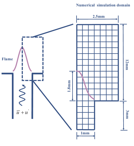
Figure 1: The configuration of numerical simulation.

3 Construction of the training dataset

To accurately construct flame nonlinear responses of single-frequency signals under any given amplitude from limited data, it is imperative to include sufficient information both for the flame dynamic responses to the oncoming flow velocity frequencies and amplitudes in the training dataset. Selecting an appropriate training dataset type that contains this information with a limited sample size is necessary. To deal with this problem, this paper uses linear frequency-sweeping signals with different amplitudes, as shown in Fig. 2.

The normalized linear frequency-sweeping velocity perturbation can be expressed as:

$$\frac{u^{\prime}(t)}{\bar{u}}=A\cos\left[2\pi\int_{t_{1}}^{t}f(t)\mathrm{d}t\right]=A\cos\left[2\pi\left(\frac{a}{2}\left(t^{2}-t_{1}^{2}\right)+b(t-t_{1})\right)\right],t\in[t_{1},t_{2}],$$ (2)

where $t_{1}$ and $t_{2}$ denote the begin and end time of each linear frequency-sweeping signal; while $f_{1}$ and $f_{2}$ represent the begin and end frequencies, respectively. $\bar{u}$ and $u^{\prime}(t)$ denote the time-averaged and perturbation of flow velocity at the inlet of the burner. $A$ denotes the normalized perturbation amplitude. $a=(f_{2}-f_{1})/(t_{2}-t_{1})$ and $b=(t_{2}f_{1}-t_{1}f_{2})/(t_{2}-t_{1})$. Herein, the frequency increases linearly with time and can be calculated by $f(t)=a~{}t+b$.

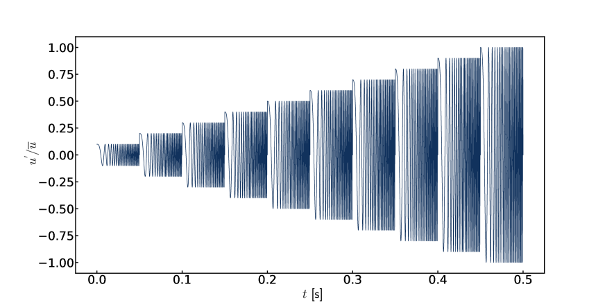
Figure 2: The schematic of frequency-sweeping signals with different amplitudes.

To ensure sufficient information for the oncoming flow velocity perturbation amplitudes $A$, we consider ten groups of linear frequency-sweeping velocity perturbations with different $A$, ranging from 0.1 to 1 with a step of 0.1. The frequencies of each group signal increase linearly from 10 Hz to 1000 Hz, encompassing all frequency information in the interested frequency range and guaranteeing sufficient frequency information. This type of dataset enables us to incorporate sufficient information both for the flame nonlinear dynamic responses to the oncoming flow velocity frequencies and amplitudes in limited data, eliminating the need to obtain single frequency signals with varying amplitudes and frequencies separately via the high-fidelity numerical simulations. Thus, the use of frequency-sweeping signals with different amplitudes greatly reduces the cost of acquiring the dataset from the numerical simulation, while containing a wealth of information in limited data.

The numerical simulations of each group utilized in this study have a duration of 0.056s and a sampling interval of $\Delta t=1\times 10^{-6}$ s for the time series, after the numerical simulation, we generate the training sample pair $(U^{\prime}\in\mathbb{R}^{6000},q^{\prime}\in\mathbb{R}^{1})$ following Eq.3, because the sample length $n$ (details about how to determine the $n$ is shown in Sec.5) is 6000 in this study, so we can generate 50,000 training sample pair for each group, consider we have ten groups, the training dataset has a total of 500,000 sample pair.

$$q^{\prime}(t)=f(u^{\prime}(t-(n-1)dt),u^{\prime}(t-(n-2)dt),\ldots,u^{\prime}(t))$$ (3)

It is worth noting that, our training set and test set are not from the same dataset as the traditional deep learning tasks. Our training data are the linear frequency-sweeping signal with different amplitudes, using this signal as training data we can train a neural network that performs well with a limited amount of data. Test data are the single-frequency signals at defined amplitudes, as thermoacoustic instabilities typically feature pure tone oscillations, the trained neural network is then validated by using the single-frequency signals at defined amplitudes as the input. The resulting heat release rate is then compared to the result from the numerical simulation.

4 Neural network model

To construct an effective neural network, it is important to design a network architecture that matches the characteristics of the training data, thereby allowing for optimal learning results. For velocity perturbation sequences, three characteristics must be considered. First, the input velocity perturbation data are time series data, and the temporal relationships between any two instances in the sequence are important for accurate predictions of the global heat release rate. Therefore, the use of a sequential neural network model (like Long Short-Term Memory (LSTM) [42] and Transformer network [43]) is essential to accurately capture these temporal dependencies.

Second, because of the influence of systems characterized by long histories, the input velocity perturbation sample has a very long length (for example, the length of a velocity perturbation sample in this study is 6000), which poses a challenge for training sequence models [44, 45]. Extreme sequence length introduces the risk of gradient vanishing in LSTM (the limiting length is less than 1000[46], and the reasonable length is 250 to 500 often used in practice with large LSTM model[47]) and increases computational complexity within Transformer architectures that rely on self-attention mechanisms [43, 48]. As a result, it is not practical to directly feed the unprocessed original sequence into the learning model, which requires a prior reduction of the sequence length before feeding into the sequence model.

Third, the low-level features are important for the accuracy and generalization ability of the neural network modeling the nonlinear flame response. Changing a single instance value or changing the time order between two instances in the input velocity perturbation sequence will affect the heat release rate. Therefore, it is important to capture these changes in different input sequences. For deep neural networks, extracted features closer to the input layer tend to contain more detailed information related to the original input features; these features, often referred to as “low-level features”, are unique to shallow layers of the network and have not yet propagated to deeper layers. Given their ability to contain more detailed information about the original sequence (this detailed information contains the more detailed changes in values and temporal at different instances of a velocity perturbation sequence, and the difference of the response of the flame is due to these changes), we believe it is helpful for constructing the flame nonlinear response.

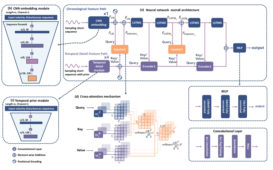
Figure 3: Overall architecture of the neural network. “Avg-Pooling” means the averaged pooling.

To address the three problems outlined above, our previous work introduced a neural network architecture featuring a combination of a Decreasing Sequence Increasing Dimension (DSID) module and a sequence module [49], which effectively addresses the first two problems. To address the third problem, based on the previous work, the present study introduces a Dual-Path model, which aims to utilize low-level features within the sequence features to improve both the accuracy of flame nonlinear response construction and the generalization ability of the neural network. Fig. 3 shows the overall architecture of the Dual-Path model, which consists of two primary components: the Chronological Features Path (CFP) and the Temporal Detail Feature Path (TDFP). The former is tasked with extracting chronological features and consists primarily of a Convolutional Neural Network (CNN) embedding module and four LSTM layers. The latter is focused on temporal detail feature extraction and includes a temporal detail module and two encoder modules. The other important module is the injector module, which built a bridge between the two paths for the interaction of features between the two paths. The Dual-Path Model mainly leverages three fundamental neural network architectures in this study: CNN [50], Recurrent Neural Network (RNN) [51], and Transformer [43]. Detailed descriptions of these models can be found in the Supplementary Materials A or reference [50, 51, 43].

The forward propagation process of the sequence features in the Dual-Path model is illustrated in Fig. 3 (a). The input velocity perturbation sequence comprises $n$ instances of velocity perturbations, each with a feature dimension of 1. Initially, the original velocity perturbation sequence is sampled into a short sequence (the details about the short sequence sampling methods is shown in Sec. 5). The short sequences are then fed into two paths for learning: the CFP and the TDFP. The CFP initiates by feeding the sequence through the CNN-embedding module to reduce the sequence length. After processing through the CNN-embedding module, the positional encoding (adding temporal information to features, the details about it can reference [43]) and features output from the Injector module are incorporated with the sequence features from the CNN-embedding module. Subsequently, these sequence features are fed into the LSTM layers to extract chronological features, with four LSTM layers being employed. The design motivation and details about the CFP are shown in Supplementary Materials B.

For the TDFP, the short sequence with prior information (the details about the prior is shown in Sec. 5) is processed by a Temporal detail module, followed by the addition of positional encoding to the output features from this module. The features enriched with more detailed temporal characteristics and prior information are utilized as key and value inputs to the Injector module while simultaneously as query inputs to the Encoder module. This study incorporates two Injector modules and two Encoder modules. The Injector module, tasked with feature interaction, accepts queries from the CFP and keys and values from the TDFP, subsequently adding the processed features back to the CFP. The Encoder module is also responsible for feature interaction, contrary to the Injector, it accepts keys and values from the CFP and queries from the TDFP. The positional arrangement of these two Injector and two Encoder modules within the overall neural network is depicted in Fig. 3 (a). Finally, the features extracted by Encoder2 and the feature corresponding to the last step of LSTM4 are combined and fed into a Multi-Layer Perceptron (MLP) module [52] for mapping to the output dimension. Given that the desired output is the global heat release rate at a certain instance, the MLP module is responsible for projecting the learned features to one value. The design motivation and details about the TDFP are shown in Supplementary Materials C.

5 Short sequence sampling

The relationship between the velocity perturbation sequence and the global heat release rate of flame response is a many-to-one connection. Specifically, the velocity perturbations constituting $n$ instances, and all the $n$ instances perturbations can influence the global heat release rate at the $t$-th instance, as depicted in Eq.(3).

The value of $n$ is contingent on the time-delay attributes inherent to the flame model. To determine the optimal value of $n$, a step function signal is employed, as illustrated in Figure 4(a). A step function signal is inputted, and then the time range of the heat release rate signal fluctuation is observed. The impact time, $\Delta t$, is estimated by the interval $t_{2}-t_{0}$. The value of $n$ is subsequently calculated as $n=\frac{\Delta t}{dt}$.

Given that the input velocity perturbations sample is very long when using the neural network to learn the flame nonlinear response, we propose a short sequence sampling methodology from the perspective of mitigating data redundancy. This approach can significantly reduce the time required for the training and inference phases of the neural network. The original input sequence, featuring $n$ velocity perturbation instances, is considered redundant, as the adjacent instances show only slight changes. Consequently, we consider that the flame response can be obtained by training the neural network on a shorter sparse sequence. To this end, we introduce a short sequence sampling method, adopting equal interval sampling for the CFP and sparse-to-dense sampling for the TDFP. The equal interval sampling means that the time intervals between consecutive sampling points remain consistent. The sparse-to-dense sampling, as illustrated in Fig. 4 (b), means sampling from front to back on the input sequence in a sparse-to-dense manner. Eq. (4) governs the sampling intervals.

$$\left\{\begin{matrix}\begin{aligned} &dn=2n/(1+n_{s})n_{s}\\ &\Delta n_{i}=\Delta n_{i-1}-dn\\ &index_{i}=\text{int}(index_{i-1}+\Delta n_{i})\\ &\Delta n_{1}=n_{s}\times dn,\;index_{1}=0\end{aligned}\end{matrix}\right.$$ (4)

In the equation above, $n$ denotes the original sequence length, $index_{i}$ denotes the sampling index of the $i$-th value in the short-sequence, int() denotes the operation of fetching the integer part, and $n_{s}$ denotes the length of the sampling short-sequence. The sampling step $\Delta n$ starts large and gradually decreases over time, resulting in a sparse-to-dense distribution of sampling indices. This choice of sampling method is motivated by the unequal impact of $n$ instances’ velocity perturbations on the global heat release rate at the $t_{n}$ instance, as visually depicted in Fig. 4(b). The closer a velocity perturbation is to the $t_{n}$ instance, the stronger its influence on the heat release rate at that instance. Conversely, the farther away from the $t_{n}$ instance, the weaker the influence.

This phenomenon is demonstrated in Fig. 4(a), where a velocity step signal transitions from a stable velocity of 1 to 1.5, resulting in a significant change in the heat release rate. Specifically, the heat release rate experiences a dramatic change from $t_{0}$ to $t_{1}$, after which the changes become smaller, and the rate maintains a stable state beyond $t_{2}$. Consequently, the impact time frame for each velocity perturbation instance on the output can be defined as $\Delta t=t_{2}-t_{0}$, with the impact on the output decreasing over time within this frame.

Therefore, we suggest the adoption of a sparse-to-dense sampling approach within the TDFP, which features fewer sampling points for the earlier instances and a greater number of sampling points for the later instances. This approach differs from equal interval sampling because it incorporates a priori knowledge of the flame’s response, i.e., that velocity perturbations at later instances have a stronger effect on the heat release rate perturbation. Sampling in this way allows the model to pay more attention to data from later instances and enhance the accuracy of the prediction results. To validate the efficacy of this approach compared to equal interval sampling, we have conducted tests using several single-frequency signals with amplitudes ranging from 0.25 to 0.95 with a step of 0.1 and each amplitude corresponding to frequencies of 100 to 900 Hz with a step of 100 Hz, resulting in a total of 72 single-frequency signals. Statistical analyses of the prediction accuracy for these 72 signals reveal that this sparse-to-dense sampling approach reduces the Mean Relative Error (MRE) by 1.2% compared to the equal interval sampling method implemented in the TDFP. The MRE is obtained from Eq. (5); $q_{i}^{\prime}$ is the $i$-th instance’s result of numerical simulation, and $\hat{q}_{i}^{\prime}$ is the $i$-th instance’s result of the neural network. In addition, the sampling short-sequence can promote the training and inference speed significantly, while at the same time the prediction accuracy is not lost or even improved. In this study, we sample the original long-sequence of length 6000 as a short-sequence of length 1000, the test results show that the training and inference speed are enhanced by 15.4 and 7.7 times respectively.

$$\text{ MRE }=\frac{\frac{1}{m}\sum_{i=1}^{m}\left|q_{i}^{\prime}-\hat{q}_{i}^{\prime}\right|}{\frac{1}{m}\sum_{i=1}^{m}|q_{i}^{\prime}|}$$ (5)

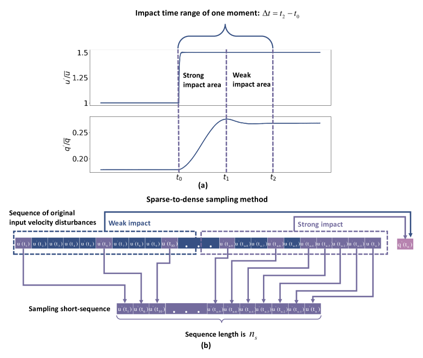
Figure 4: (a) Flame dynamic response to the step function signal. (b) Schematic diagram of short sequence sampling method; $n$ and $n_{s}$ are the lengths of the original sequence and the sampling short sequence, respectively.

6 Validation results

6.1 Implementation details

The implementation is conducted on PyTorch [53]. Datasets are obtained from the numerical simulation mentioned in Sec.2 and the signal type of training dataset uses a frequency-sweeping signal proposed in Sec.3. During the training process, in the convolutional neural network layers and fully connected layers, we add BatchNorm [54] to calculate the mean and variance of each layer to adjust the data distribution at each layer. That can make training more stable and speed up the training process. As for the optimizer, we use the Adam optimizer [55] with $\beta_{1}=0.9$, $\beta_{2}=0.999$, $\varepsilon=10^{-9}$, and weight decay is set to 0.01. The initial learning rate is $10^{-4}$, following PyTorch’s MultiStepLR method to change the learning rate, milestones are set to [40,80,90], and gamma is set to 0.1. The configurations for our neural network model are set as shown in Table 1. The loss function uses MSE as shown in Eq. (6); $\hat{q}_{i}^{\prime}$ is the output value of the neural network, and $q_{i}^{\prime}$ is the result produced by numerical simulation.

$$\text{ MSEloss }=\frac{1}{n}\sum_{i=1}^{n}\left(q_{i}^{\prime}-\hat{q}_{i}^{\prime}\right)^{2}$$ (6)

Table 1: Configurations for our neural network model. “conv” means the convolution layer, “number of heads” means the heads number of multi-head attention, “FFN dimensions” means the expanded feature dimensions of position-wise FFN layer.

Chronological Feature Path	Temporal Detail Feature Path	MLP
CNN-embedding: 3$\times$1 conv, 32 channels, stride 1 2$\times$2 average pool, stride 2 3$\times$1 conv, 64 channels, stride 1 2$\times$2 average pool, stride 2 3$\times$1 conv, 128 channels, stride 1 2$\times$2 average pool, stride 2 3$\times$1 conv, 128 channels, stride 1 2$\times$2 average pool, stride 2 LSTM: 128 in_features, 128 hidden_features 128 in_features, 128 hidden_features 128 in_features, 128 hidden_features 128 in_features, 128 hidden_features	Temporal detail module: 3$\times$1 conv, 64 channels, stride 1 2$\times$2 average pool, stride 2 3$\times$1 conv, 128 channels, stride 1 2$\times$2 average pool, stride 2 Injector1/Injector2: 128 in_features, 128 out_features number of heads 1 Encoder1/Encoder2: 128 in_features, 128 out_features FFN dimensions 256 number of heads 4	128 in_features, 64 out_features 64 in_features, 32 out_features 32 in_features, 1 out_features

6.2 Construction capability of flame nonlinear response

This section demonstrates the abilities of the Dual-Path model in constructing the flame nonlinear response for numerical simulations. Considering MLP is the most classic model and LSTM is the most classic sequence model applied in deep learning, we have compared the construction ability of the Dual-Path model with the two models. In order to prove the better prediction accuracy of Dual-Path is not due to the simple addition of model learnable parameters, we set the learnable parameters of MLP, LSTM, and Dual-Path model to the same order of magnitude. Specifically, the sum of parameters of MLP, LSTM, and Dual-Path model are 1050379, 1017692, and 1043137, the sum of the parameters can be obtained from Pytorch’s function. The MLP has four layers, the input and output features of each layer are [6000,170], [170,128], [128,64], and[64,1] respectively, and the dropout rate is 0.5. The LSTM has also four layers, the input and output features of each layer are [1,300], [300,256], [256,64], and [64,1] respectively, and the dropout rate is 0.3.

The prediction results in the time domain obtained at various velocity perturbation amplitudes (0.25, 0.55, and 0.85) and frequencies (200 Hz, 400 Hz, 600 Hz, and 800 Hz for each amplitude), are presented in Figs.5, 6, and 7. These figures demonstrate the robust performance of the Dual-Path model in predicting the flame nonlinear response across different single-frequency signals. Especially for frequencies of 600Hz, the prediction performance of MLP and LSTM is poor relative to the Dual-Path model, which proves the Dual-Path model has a more powerful nonlinear capture capability (600Hz performs stronger nonlinearity). These three figures also show that LSTM has a better performance than MLP, which may be due to LSTM’s ability to capture temporal features that MLP does not have.

To quantify the model’s accuracy across various single-frequency signals in the time domain, we have conducted statistical assessments using the MRE, as shown in Fig. 8. Fig. 8 has shown the prediction performance of the Dual-Path model, which includes signals with amplitudes ranging from 0.25 to 0.95 with a step of 0.1, and each amplitude corresponds to frequencies from 100 Hz to 900 Hz with a step of 100 Hz. In total, there are 72 different single-frequency signals included in Fig. 8. From Fig. 8 we can see that almost all signals’ MRE are under 10%, and we have also calculated the average MRE of the 72 signals, the result shows that our method achieves an average MRE of around 6.69%. For comparison, the average MRE of MLP is around 23.85% and LSTM is around 12.50%, the details of the MRE of MLP and LSTM for 72 signals are shown in Fig.S11 and S12 respectively. Another worth noting is that the training and inference time of LSTM is enormous if directly feeds the original velocity perturbation sequence to LSTM. MLP takes the least amount of training and inference time, and the training time of the Dual-Path model is around 11 times of MLP and the inference time is around 180 times of MLP. However, the training time of LSTM is around 205 times of MLP and the inference time is around 5000 times of MLP. Therefore, only using LSTM to construct flame nonlinear response is not a good choice either for training and inference costs or for prediction accuracy. These above results demonstrate the Dual-Path’s capacity to predict the flame nonlinear response accurately for a wide range of single-frequency signals, thereby constructing a precise flame nonlinear response.

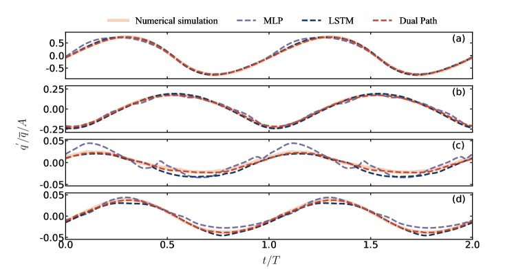
Figure 5: Comparison of prediction results between different neural network models when $A=0.25$. From (a) to (d), the perturbation frequencies are 200 Hz, 400 Hz, 600 Hz, and 800 Hz, respectively. The original input sequence length $n$ is 6000, and the short sequence sampling length $n_{s}$ is set to 1000. $T$ and $A$ denote the period and amplitude of each signal respectively.

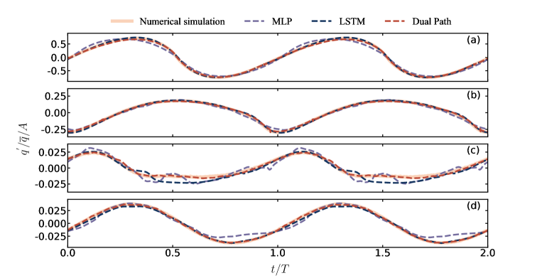
Figure 6: Comparison of prediction results between different neural network models when $A=0.55$. The remaining details are identical to those described in the caption of Fig. 5.

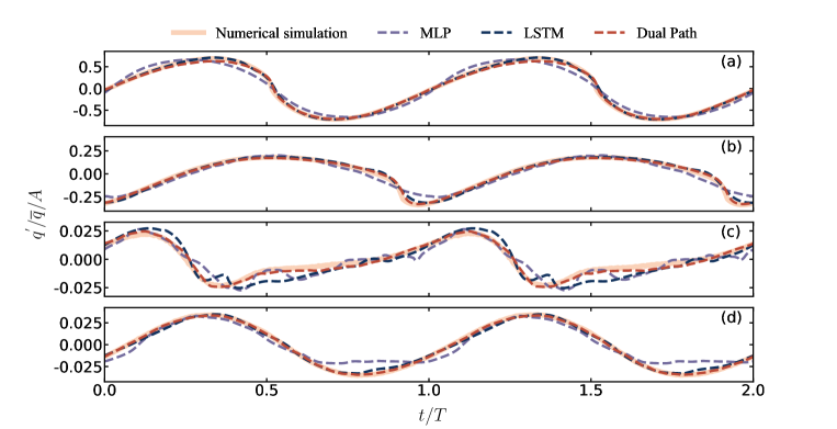
Figure 7: Comparison of prediction results between different neural network models when $A=0.85$. The remaining details are identical to those described in the caption of Fig. 5.

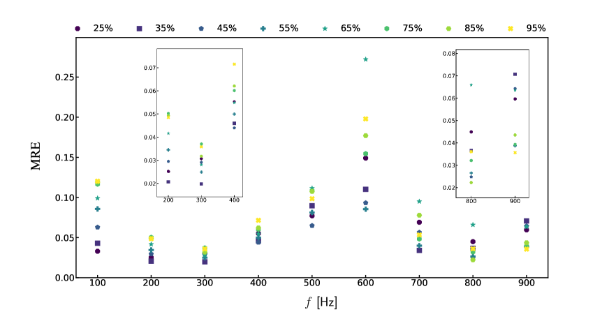
Figure 8: The MRE of single-frequency signals of Dual-Path model with different amplitudes ($A$ equals the value after the marker at the top of the figure) and frequencies.

However, as shown in Fig. 8, the predicted results at 600 Hz are relatively poor compared to those at other frequencies. We revisited the results of the numerical simulation of the sweep signal in the range of 10 - 1000 Hz, as shown in Fig. 9. This figure revealed a distinctive nonlinearity in the output of the sweeping signal within the range of 510 Hz to 660 Hz, which is different from the behavior exhibited in other frequency ranges, and this distinctiveness is only a small fraction of the training dataset. Consequently, the neural network lacks sufficient data to effectively learn mapping relationships within this particular frequency range of 510 Hz to 660 Hz. As a result, the learned mapping relations within the neural network tend to align with other frequency ranges, leading to poorer performance in this particular frequency range. However, it is worth noting that the Dual-Path model proposed in this study demonstrates robust generalization capabilities when compared to other neural networks (MLP and LSTM), as shown in Figs.5, 6, and 7. In order to prove TDFP can enhance the generalization capabilities of the Dual-Path model, we have compared the prediction performance of special data distribution with the Single-Path model(which comprises only a CFP and has no TDFP), as illustrated in Supplementary Material E. For the special data distribution in the 510 Hz to 660 Hz frequency range, the Single-Path neural network models fail to achieve comparable performance compared to the Dual-Path model, which proves that the TDFP is important for the generalization capabilities of the model. It is also worth noting that When the flame nonlinear response does not exhibit this special data distribution, our method excels at predicting responses across all frequencies, as shown in Supplementary Material F.

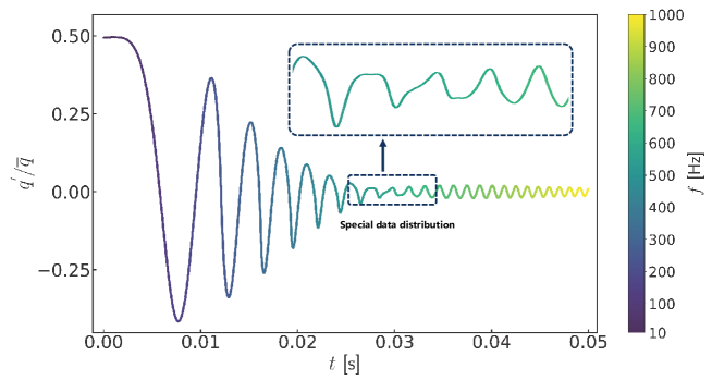
Figure 9: Heat release rate results of the frequency-sweeping signal of numerical simulation, the amplitude of the frequency-sweeping is $A=0.5$ and the range of the frequencies are 10 - 1000 Hz.

In addition to the special data distribution within the frequency range of 510 Hz to 660 Hz, another special data distribution is small amplitude-high frequency (SAHF) signals, for example, the signals with amplitudes of 0.1 and frequencies ranging from 700 Hz to 900 Hz. Figs.10 illustrates that the predicted results for SAHF signals exhibit poor performance. This is because the data distribution range of heat release rate values of SAHF signals deviates significantly from the overall distribution of the training dataset. Specifically, these values are too small in comparison to the distribution of the whole dataset. As depicted in Figs. 11, the heat release rate values for an amplitude of 0.1 in the high-frequency region are relatively substantially smaller and exhibit minimal fluctuation compared to higher amplitudes (0.5 and 1). This substantial deviation from the overall data distribution presents a challenge in capturing precise flame responses for SAHF signals. However, the Dual-Path model outperforms the Single-Path model when predicting the flame response of SAHF signals, as shown in Supplementary Material E. This highlights the Dual-Path model’s robust generalization capabilities and the importance of TDFP, enabling it to handle specialized data distributions effectively.

To further enhance the prediction accuracy of SAHF signals, we leverage transfer learning techniques [56, 57]. Given that the Dual-Path model, trained with 0.5 seconds of numerical simulation data as proposed in Sec. 3, has already acquired knowledge of general flame nonlinear response patterns, we choose to fine-tune a small number of parameters of the model with limited data to enhance the accuracy of predictions for SAHF signals. Fig. 12 shows our approach, where we freeze the parameters of all model components except for the MLP module, as we believe that these parameters encapsulate general flame nonlinear response patterns. Fine-tuning these parameters could potentially destroy these patterns. So we only fine-tune the MLP module using a small dataset of short-duration SAHF signals. For example, we fine-tune the model using two 0.01s single-frequency time series with an amplitude of 0.1 at frequencies of 800 Hz and 900 Hz. After fine-tuning, the model can have a better prediction of all responses from the 800 Hz to 900 Hz , as demonstrated in Supplementary Material G. Notably, transfer learning requires only a limited amount of data for fine-tuning specific neural network parameters and does not significantly increase training time. Therefore, we consider it a cost-effective approach to enhance the prediction accuracy of SAHF signals.

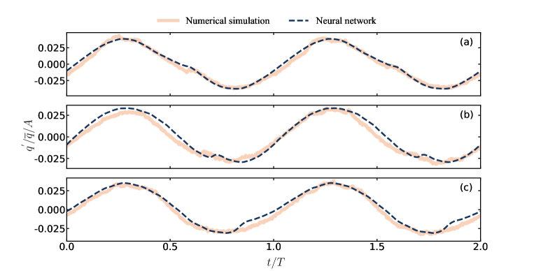
Figure 10: Comparison of prediction results of Dual-Path model and numerical simulation. $A=0.1$, and $f$ are 700 Hz, 800 Hz, and 900 Hz from $(a)$ to $(c)$. $n$=6000, $n_{s}$=1000.

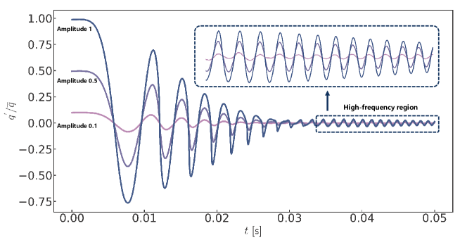
Figure 11: Comparison of heat release rate results for frequency-sweeping signals of different amplitudes. The amplitudes are 0.1, 0.5, and 1, and the frequencies are swept from 10 to 1000 Hz.

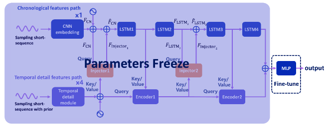
Figure 12: Schematic of transfer learning

6.3 Construction capability of the strong nonlinear response of the flame

Sec. 6.2 has shown the construction capability of flame nonlinear response. However, the level of nonlinearity in the flame response is not strong, and in this section, we aim to investigate the ability of the Dual-Path model to construct the flame response with strong nonlinearity. It is worth noting that the strong nonlinear response of flame is different from the special nonlinear data distribution in the 510 to 600 Hz presented in Sec.6.2, the former means that all frequency ranges in the training dataset are strong nonlinear distribution and the later is only a small part of the overall training dataset. To achieve this goal, we conduct a verification process, similar to our previous work [49], using the modified classical $n-\tau$ model [58]. This model is chosen due to its ability to easily adjust the level of nonlinearity compared to numerical simulations. The expression for the $n-\tau$ model is as follows:

$$\frac{q^{\prime}(t)}{\bar{q}}=\frac{\omega_{c}}{s+\omega_{c}}*\left\{a_{1}\frac{u^{\prime}\left(t-\tau_{u_{1}}\right)}{\bar{u}}-a_{3}\left(\frac{u^{\prime}\left(t-\tau_{u_{3}}\right)}{\bar{u}}\right)^{3}\right\}$$ (7)

The angular cutoff frequency of a first-order filter is denoted by $\omega_{c}=2\pi f_{c}$, where $s=\mathrm{i}\omega=\mathrm{i}2\pi f$ represents the Laplace variable. Dimensionless constants $a_{1}$ and $a_{3}$, along with time delay terms $\tau_{u_{1}}$ and $\tau_{u_{3}}$, are also included in the model. The symbol $\ast$ indicates convolution. In this study, we set $f_{c}=400$ Hz, $\tau_{u_{1}}=\tau_{u_{3}}=2$ ms, and $a_{1}=1$. Equation (7) is employed to generate the heat release rate for both the training and test sets. The cubic term in this equation introduces nonlinearity, the strength of which is adjustable by varying the ratio $a_{3}/a_{1}$. As this ratio increases, so does the nonlinearity strength. We established a range for $a_{3}/a_{1}$ as [1, 2, 3, 4, 5], with the maximum ratio capped at 5 to prevent the cubic term from overwhelming and distorting the model’s physical interpretation. Figure 13 illustrates the neural network’s prediction results across different nonlinearity strengths, with each strength trained independently. These results confirm the neural network’s capability to accurately construct the flame’s nonlinear response, even at very high nonlinearity strengths.

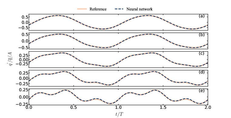
Figure 13: Prediction results of neural networks for different nonlinear strengths of flames. From $(a)$ to $(e)$, the ratios $a_{3}/a_{1}$ are 1, 2, 3, 4, and 5. The sample size of the training dataset used is 100,000. The amplitude of the input signal is 0.45, and the frequency is 350 Hz. Orange solid line: the results produced by Eq. (7). Blue dashed line: the results predicted by neural networks.

Our proposed method has shown excellent performance in accurately constructing the flame nonlinear response at any nonlinear strength. However, the cost of construction varies depending on the strength of nonlinearity, as different nonlinear strengths require varying training dataset sizes for precise construction. To further investigate the effect of training dataset size and nonlinear strengths, Fig. 14 shows the average MRE on 10 single-frequency signals. The frequencies of these signals range from 100 to 1000 Hz with a step of 100 Hz, and the amplitude of these signals is 0.5 because it causes significant nonlinearity. The horizontal axis represents the training dataset size, while the vertical axis represents the average MRE between the neural network prediction results and the numerical simulation results. Fig. 14 shows that for the same training dataset size, the MRE increases with increasing the nonlinear strength. However, for the same nonlinear strength, the MRE decreases with increasing the dataset size. This suggests that providing more training data samples improves the learning effect of the neural network model. Strong nonlinearities require more data to capture their mapping relationships due to their complex and intricate mapping relationships, which require more data to explore fully. If the nonlinearity is not strong, a small training dataset can achieve good performance.

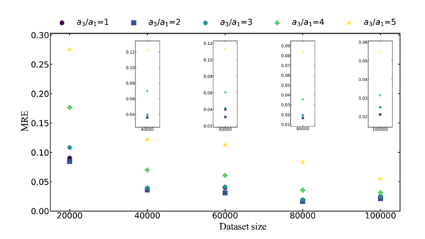
Figure 14: Statistical results of the MRE for different nonlinear strengths and the training dataset size. The nonlinear strengths are taken as 1, 2, 3, 4, and 5. The training dataset sizes are taken as 20000,40000, 60000,80000 and 100000.

7 Conclusion

This paper introduces a deep learning-based approach for accurately construct the nonlinear thermoacoustic response of flames in the time domain, using a limited set of numerical simulation data. The research emphasizes two primary aspects: the training datasets and the neural network models. The training datasets utilize frequency-sweeping signals of varying amplitudes, building on our prior work, which contains rich amplitude and frequency information to support the learning of neural network.

Regarding the neural network architecture, we propose a Dual-Path model consisting of a Chronological Features Path (CFP) and a Temporal Detail Feature Path (TDFP). The CFP extracts chronological features, while the TDFP enhances the model’s focus on detailed temporal features, thereby improving the network’s generalization capabilities. Results show that the proposed training dataset and Dual-Path model successfully capture the flame’s nonlinear response with limited numerical data. Additionally, the paper introduces a novel short-sequence sampling method that not only enhances the accuracy of the neural network but also significantly reduces both training and inference times, thus boosting efficiency. The effectiveness of this model is confirmed under conditions of extreme nonlinearity, proving its capability to precisely model highly nonlinear flame behaviors. The study also suggests that the size of the training dataset should correlate with the nonlinearity’s intensity, which can reduce both data collection costs and training durations for less intense nonlinearities.

References

- [1] D. Durox, T. Schuller, N. Noiray, A.-L. Birbaud, S. Candel, Rayleigh criterion and acoustic energy balance in unconfined self-sustained oscillating flames, Combust. Flame 156 (2009) 106–119.
- [2] K. T. Kim, Combustion instability feedback mechanisms in a lean-premixed swirl-stabilized combustor, Combust. Flame 171 (2016) 137–151.
- [3] Y. Huang, V. Yang, Dynamics and stability of lean-premixed swirl-stabilized combustion, Prog. Energ. Conbust 35 (2009) 293–364.
- [4] T. Poinsot, Prediction and control of combustion instabilities in real engines, Proc. Combust. Inst 36 (2017) 1–28.
- [5] G. H. Markstein, Nonsteady flame propagation: AGARDograph, Elsevier, 2014.
- [6] M. Fleifil, A. M. Annaswamy, Z. Ghoneim, A. F. Ghoniem, Response of a laminar premixed flame to flow oscillations: A kinematic model and thermoacoustic instability results, Combust. Flame 106 (1996) 487–510.
- [7] T. Lieuwen, Nonlinear kinematic response of premixed flames to harmonic velocity disturbances, Proc. Combust. Inst 30 (2005) 1725–1732.
- [8] S. Ducruix, D. Durox, S. Candel, Theoretical and experimental determinations of the transfer function of a laminar premixed flame, Proc. Combust. Inst 28 (2000) 765–773.
- [9] N. Noiray, D. Durox, T. Schuller, S. Candel, A unified framework for nonlinear combustion instability analysis based on the flame describing function, J. Fluid Mech 615 (2008) 139–167.
- [10] H. Krediet, C. Beck, W. Krebs, J. Kok, Saturation mechanism of the heat release response of a premixed swirl flame using les, Proc. Combust. Inst 34 (2013) 1223–1230.
- [11] X. Han, A. S. Morgans, Simulation of the flame describing function of a turbulent premixed flame using an open-source les solver, Combust. Flame 162 (2015) 1778–1792.
- [12] J. Li, Y. Xia, A. S. Morgans, X. Han, Numerical prediction of combustion instability limit cycle oscillations for a combustor with a long flame, Combust. Flame 185 (2017) 28–43.
- [13] W. Polifke, Black-box system identification for reduced order model construction, Ann. Nucl. Energy 67 (2014) 109–128.
- [14] T. Liu, J. Li, Y. Song, L. Yang, A weakly nonlinear analytical model for the transversely forced flame describing function of a slit flame, Fuel 292 (2021) 120247.
- [15] S. K. Thumuluru, T. Lieuwen, Characterization of acoustically forced swirl flame dynamics, Proc. Combust. Inst 32 (2009) 2893–2900.
- [16] X. Han, J. Li, A. S. Morgans, Prediction of combustion instability limit cycle oscillations by combining flame describing function simulations with a thermoacoustic network model, Combust. Flame 162 (2015) 3632–3647.
- [17] J. Li, A. S. Morgans, Time domain simulations of nonlinear thermoacoustic behaviour in a simple combustor using a wave-based approach, J. Sound Vib 346 (2015) 345–360.
- [18] T. Schuller, D. Durox, S. Candel, A unified model for the prediction of laminar flame transfer functions: comparisons between conical and v-flame dynamics, Combust. Flame 134 (2003) 21–34.
- [19] H. Wang, C. K. Law, T. Lieuwen, Linear response of stretch-affected premixed flames to flow oscillations, Combust. Flame 156 (2009) 889–895.
- [20] C. Li, D. Yang, S. Li, M. Zhu, An analytical study of the effect of flame response to simultaneous axial and transverse perturbations on azimuthal thermoacoustic modes in annular combustors, Proc. Combust. Inst 37 (2019) 5279–5287.
- [21] Y. LeCun, Y. Bengio, G. Hinton, Deep learning, Nature 521 (2015) 436–444.
- [22] S. Minaee, Y. Boykov, F. Porikli, A. Plaza, N. Kehtarnavaz, D. Terzopoulos, Image segmentation using deep learning: A survey, IEEE Trans. Pattern Anal. Mach. Intell 44 (2021) 3523–3542.
- [23] E. Arani, S. Gowda, R. Mukherjee, O. Magdy, S. Kathiresan, B. Zonooz, A comprehensive study of real-time object detection networks across multiple domains: A survey, arXiv preprint arXiv:2208.10895 (2022).
- [24] X. Qiu, T. Sun, Y. Xu, Y. Shao, N. Dai, X. Huang, Pre-trained models for natural language processing: A survey, Sci. China Technol. Sci 63 (2020) 1872–1897.
- [25] D. Khurana, A. Koli, K. Khatter, S. Singh, Natural language processing: State of the art, current trends and challenges, Multimed. Tools Appl 82 (2023) 3713–3744.
- [26] D. E. Ozan, L. Magri, Hard-constrained neural networks for modeling nonlinear acoustics, Phys. Rev. Fluids 8 (10) (2023) 103201.
- [27] M. Yoko, M. P. Juniper, Adjoint-accelerated bayesian inference applied to the thermoacoustic behaviour of a ducted conical flame, J. Fluid Mech 985 (2024) A38.
- [28] Z. Wang, W. Lin, Y. Tong, K. Guo, P. Chen, W. Nie, W. Huang, Early detection of thermoacoustic instability in an o2/ch4 single-injector rocket combustor using analysis of chaos and deep learning models, Phys. Fluids 36 (3) (2024).
- [29] S. Liu, P. Wan, X. Shang, Hasr-tai: Hybrid model-based interpretable network and super-resolution network for thermoacoustic imaging, Appl. Phys. Lett. 123 (13) (2023).
- [30] M. Raissi, P. Perdikaris, G. E. Karniadakis, Physics-informed neural networks: A deep learning framework for solving forward and inverse problems involving nonlinear partial differential equations, J. Comput. Phys. 378 (2019) 686–707.
- [31] H. Son, M. Lee, A pinn approach for identifying governing parameters of noisy thermoacoustic systems, J. Fluid Mech 984 (2024) A21.
- [32] S. Mariappan, K. Nath, G. E. Karniadakis, Learning thermoacoustic interactions in combustors using a physics-informed neural network, arXiv preprint arXiv:2401.00061 (2023).
- [33] C. F. Silva Garzon, P. Bonnaire, N. A. K. Doan, K. Niebler, C. F. Silva, Towards reconstruction of acoustic fields via physics-informed neural networks, in: INTER-NOISE and NOISE-CON Congress and Conference Proceedings, Vol. 265, Institute of Noise Control Engineering, 2023, pp. 4773–4782.
- [34] D. E. Ozan, L. Magri, Physics-aware learning of nonlinear limit cycles and adjoint limit cycles, in: INTER-NOISE and NOISE-CON Congress and Conference Proceedings, Vol. 265, Institute of Noise Control Engineering, 2023, pp. 1191–1199.
- [35] S. Jaensch, W. Polifke, Uncertainty encountered when modelling self-excited thermoacoustic oscillations with artificial neural networks, Int. J. Spray Combust 9 (2017) 367–379.
- [36] N. Tathawadekar, N. A. K. Doan, C. F. Silva, N. Thuerey, Modeling of the nonlinear flame response of a bunsen-type flame via multi-layer perceptron, Proc. Combust. Inst 38 (2021) 6261–6269.
- [37] V. Yadav, M. Casel, A. Ghani, Physics-informed recurrent neural networks for linear and nonlinear flame dynamics, Proc. Combust. Inst (2022).
- [38] E. Gonzalez, Numerical simulations of thermoacoustic combustion instabilities in the volvo combustor, in: 53rd AIAA/SAE/ASEE Joint Propulsion Conference, 2017, p. 4686.
- [39] Q. Yang, P. Zhao, H. Ge, reactingfoam-sci: An open source cfd platform for reacting flow simulation, Comput. Fluids 190 (2019) 114–127.
- [40] O. A. Marzouk, E. D. Huckaby, A comparative study of eight finite-rate chemistry kinetics for co/h2 combustion, Eng. Appl. Comput. Fluid Mech 4 (2010) 331–356.
- [41] M. V. Petrova, F. A. Williams, A small detailed chemical-kinetic mechanism for hydrocarbon combustion, Combust. Flame 144 (2006) 526–544.
- [42] S. Hochreiter, J. Schmidhuber, Long short-term memory, Neural. Comput 9 (1997) 1735–1780.
- [43] A. Vaswani, N. Shazeer, N. Parmar, J. Uszkoreit, L. Jones, A. N. Gomez, Ł. Kaiser, I. Polosukhin, Attention is all you need, Adv. Neural Inf. Process. Syst 30 (2017).
- [44] Y. Bengio, P. Simard, P. Frasconi, Learning long-term dependencies with gradient descent is difficult, Int. J. Neural Netw 5 (1994) 157–166.
- [45] R. Pascanu, T. Mikolov, Y. Bengio, On the difficulty of training recurrent neural networks, in: Int. Conf. Mach. Learn, Pmlr, 2013, pp. 1310–1318.
- [46] S. Li, W. Li, C. Cook, C. Zhu, Y. Gao, Independently recurrent neural network (indrnn): Building a longer and deeper rnn, in: Proceedings of the IEEE conference on computer vision and pattern recognition, 2018, pp. 5457–5466.
- [47] S. Kumari, N. Kumar, P. S. Rana, Big data analytics for energy consumption prediction in smart grid using genetic algorithm and long short term memory., Computing & Informatics 40 (1) (2021).
- [48] Y. Tay, M. Dehghani, D. Bahri, D. Metzler, Efficient transformers: A survey, ACM Comput. Surv 55 (2022) 1–28.
- [49] J. Wu, J. Nan, L. Yang, J. Li, Reconstruction of the flame nonlinear response using deep learning algorithms, Phys. Fluids 35 (2023) 017125.
- [50] Y. LeCun, L. Bottou, Y. Bengio, P. Haffner, Gradient-based learning applied to document recognition, Proc. IEEE 86 (1998) 2278–2324.
- [51] J. L. Elman, Finding structure in time, Cogn. Sci 14 (1990) 179–211.
- [52] K. Hornik, Approximation capabilities of multilayer feedforward networks, Neural Netw 4 (1991) 251–257.
- [53] A. Paszke, S. Gross, F. Massa, A. Lerer, J. Bradbury, G. Chanan, T. Killeen, Z. Lin, N. Gimelshein, L. Antiga, et al., Pytorch: An imperative style, high-performance deep learning library, Adv. Neural Inf. Process. Syst 32 (2019).
- [54] S. Ioffe, C. Szegedy, Batch normalization: Accelerating deep network training by reducing internal covariate shift, in: Int. Conf. Mach. Learn, pmlr, 2015, pp. 448–456.
- [55] D. P. Kingma, J. Ba, Adam: A method for stochastic optimization, arXiv preprint arXiv:1412.6980 (2014).
- [56] S. J. Pan, Q. Yang, A survey on transfer learning, IEEE Trans. Knowl. Data Eng 22 (2009) 1345–1359.
- [57] K. Weiss, T. M. Khoshgoftaar, D. Wang, A survey of transfer learning, J. Big Data 3 (2016) 1–40.
- [58] L. Yang, B. Pang, J. Li, Comparison of strongly and weakly nonlinear flame models applied to thermoacoustic instability, Phys. Fluids 33 (2021) 094108.