Syntax-Guided Procedural Synthesis of Molecules

Abstract

Designing synthetically accessible molecules and recommending analogs to unsynthesizable molecules are important problems for accelerating molecular discovery. We reconceptualize both problems using ideas from program synthesis. Drawing inspiration from syntax-guided synthesis approaches, we decouple the syntactic skeleton from the semantics of a synthetic tree to create a bilevel framework for reasoning about the combinatorial space of synthesis pathways. Given a molecule we aim to generate analogs for, we iteratively refine its skeletal characteristics via Markov Chain Monte Carlo simulations over the space of syntactic skeletons. Given a black-box oracle to optimize, we formulate a joint design space over syntactic templates and molecular descriptors and introduce evolutionary algorithms that optimize both syntactic and semantic dimensions synergistically. Our key insight is that once the syntactic skeleton is set, we can amortize over the search complexity of deriving the program’s semantics by training policies to fully utilize the fixed horizon Markov Decision Process imposed by the syntactic template. We demonstrate performance advantages of our bilevel framework for synthesizable analog generation and synthesizable molecule design. Notably, our approach offers the user explicit control over the resources required to perform synthesis and biases the design space towards simpler solutions, making it particularly promising for autonomous synthesis platforms.

1 Introduction

The discovery of new molecular entities is central to advancements in fields such as pharmaceuticals [72, 40], materials science [26, 31], and environmental engineering [73, 67]. Traditional make-design-test workflows for molecular design typically rely on labor-intensive methods that involve a high degree of trial and error [52]. Systematic and data-efficient approaches that minimize costly experimental trials are the key to accelerating these processes [11, 12, 22]. In recent years, a large number of molecular generative models has been proposed [15, 41, 55, 68, 38, 51, 39, 32, 33, 25, 59]. However, few of their outputs are feasible to make and proceed to experimental testing due to their lack of consideration for synthesizability [20]. This has motivated methods that integrate design and synthesis into a single workflow, aiming to optimize both processes simultaneously [65, 27, 6, 2, 3, 21, 60] which significantly closes the gap between the design and make steps, reducing cycle time significantly [36, 66, 43]. These methods still face computational challenges, particularly in navigating the combinatorial explosion of potential synthetic pathways [56].

Inspired by techniques in program synthesis, particularly Syntax-Guided Synthesis (SyGuS) [1], our method decouples the syntactical template of synthetic pathways (the skeleton) from their chemical semantics (the substance). This bifurcation allows for a more granular optimization process, wherein the syntactical and semantic aspects of reaction pathways can be optimized independently yet synergistically. Our methodology employs a bilevel optimization strategy, wherein the upper level optimizes the syntactic template of the synthetic pathway, and the lower level fine-tunes the molecular descriptors within that given structural framework. This dual-layered approach is facilitated by a surrogate policy, implemented via a graph neural network, that propagates embeddings top-down following the topological order of the syntactical skeleton. This ensures that each step in the synthetic pathway is optimized in context, respecting the overarching structural strategy while refining the molecular details. We address the combinatorial explosion in the number of programs using tailored strategies for fixed horizon Markov decision process (MDP) environments. This algorithm amortizes the complexity of the search space through predictive modeling and simulation of Markov Chain Monte Carlo (MCMC) processes [47, 28, 24], focusing on the generation and evaluation of syntactical skeletons. By leveraging the inductive biases from retrosynthetic analysis without resorting to retrosynthesis search, our approach combines accuracy and efficiency in “synthesizing" synthetic pathways. In summary, the contributions of this work are:

• We reconceptualize molecule design and synthesis as a conditional program synthesis problem, establishing common terminology for bridging the two fields.

• We propose a bilevel framework that decouples the syntactical skeleton of a synthetic tree from the program semantics.

• We introduce amortized algorithms within the bilevel framework for the tasks of synthesizable analog recommendation and synthesizable molecule design.

• We demonstrate improvements across multiple dimensions of performance for both tasks.

• We include in-depth visualizations and analyses for understanding the source of our method’s efficacy as well as its limitations.

2 Related Works

2.1 Synthesis Planning

Prior works model synthetic pathways using a discrete data structure known as the synthetic tree. The root node is the target molecule, leaf nodes are building blocks, and intermediate nodes can be either reactions or intermediates. This task is to infer a synthesis tree that reconstructs a target molecule $M\in\mathcal{M}$, where $\mathcal{M}$ is the space of all molecules (estimated to be $10^{30-100}$). Retrosynthetic analysis is a branch of organic chemistry that centers around designing synthesis pathways for a target molecule through backward reasoning steps [13]. Computer-assisted retrosynthetic analysis has developed through the decades [14] in tandem with computers, and is now known as retrosynthetic planning due to its resemblance to more classical tests of AI based around planning. State-of-the-art retrosynthesis planning algorithms today use neural networks to learn complex transformation patterns over the vast space of molecular structures, and the field has gained attention in recent years [9] as machine learning has begun to transform drug discovery and materials design.

2.2 Synthesizable Analog Generation

The problem of synthesizable analog generation aims to find molecules close to the target molecule which are synthesizable. Note that the constraint of synthesizable delinates this problem from conditional molecule generation, but works such as [50] attempt to bridge these two. As retrosynthetic planning is done by working backwards (top-down), partial success is not straightforward to define. In other domains, procedural modeling is a bottom-up generation process that generates analogs by design [45, 46, 48, 44]. Thus, synthesizable analog generation has warranted more specialized methods. Prior works such as [16, 37] address this by starting from an existing retrosynthesis route, and performing alteration of the route. This constrained approach limits the diversity of analogs severely. Instead, we neither start from a search route nor constrain the search route, but instead extract analogs via iterative refinement of the program’s syntactical skeleton with inner-loop decoding of the program semantics in a bilevel setup. Our framework simultaneously handles analog generation and, as a special case, synthesis planning. We implement the iterative refinement phase using a MCMC sampler with a stationary distribution governed by similarity to the target being conditioned on. This is a common technique used to search over procedural models of buildings, shapes, furniture arrangements, etc., [46, 61, 69] and we showcase its efficacy for the new application domain of molecules.

2.3 Synthesizable Molecule Design

The problem of synthesizable molecule design is to optimize for the synthetic pathway which produces a molecule that maximizes some property oracle function. Note that unlike generic molecular optimization approaches, the design space is reformulated to guarantee synthesizability by construction. The early works to follow this formulation [65, 27, 6] use machine learning to assemble molecules by iteratively selecting building blocks and virtual reaction templates to enumerate a library, with recent works such as [60] obtaining experimental validation. The key computational challenge these methods must address is how to best navigate the combinatorial search space of synthetic pathways. Prior works that do bottom-up generation of synthetic trees [2, 3] probabilistically model a synthetic tree as a sequence of actions. These works adopt an encoder-decoder approach to map to and from a latent space, e.g., using a VAE, assuming a smooth mapping between continuous latent space to a complex and highly discontinuous combinatorial space. This results in low reconstruction accuracy, hindering the method on the task of conditional generation. SynNet [21] instead formulates the problem as an infinite-horizon MDP and do amortized tree generation conditioned on a Morgan fingerprint. This enables a common framework for solving both tasks. However, we show improvements on both analog generation and synthesizable molecule design in terms of reconstruction accuracy and diversity through our novel formulation.

2.4 Program Synthesis

Program synthesis is the problem of synthesizing a function $f$ from a set of primitives and operators to meet some correctness specification. A program synthesis problem entails: a background theory $\mathsf{T}$ which is the vocabulary for constructing formulas, a correctness specification: a logical formula involving the output of $f$ and $\mathsf{T}$, and a set of expressions $L$ that $f$ can take on described by a context-free grammar $G_{L}$. In molecular synthesis, we can formulate $\mathsf{T}$ as containing operators for chemical reactions, constants for reagents, molecular graph isomorphism checking comparisons, etc. The correctness specification for finding a synthesis route for $M$ is simply $f(\{B\})=M$ (where $\{B\}$ is a set of building blocks) and we seek to find an implementation $f$ from $L$ to meet the specification. A related but coarser specification is to match the fingerprint $X$ of some molecule: $FP(f(\{B\}))=X$, and as shown by [21], this relaxed formulation enables both analog generation and GA-based molecule optimization. Our key innovation takes inspiration from the line of work surrounding syntax-guided synthesis [1, 53] (SyGuS). Syntax guidance explicitly constrains $G_{L}$ which reduces the set of implementations $f$ can take on [1], enabling more accurate amortized inference. Further discussion on the connections between program synthesis and molecular synthesis is in App C.

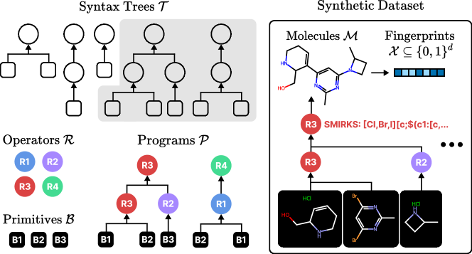
Figure 1: We introduce program synthesis terminology for modeling synthesis pathways.

3 Methodology

3.1 Problem Definition

Synthesis Planning

This task is to infer the program as well as the inputs that reconstructs a target molecule. When the outcome is binary (whether a certificate to exactly reconstruct the target is found), this problem is known as synthesis planning. When the outcome can be between 0 and 1, e.g., similarity to target molecule, this problem is known as synthesizable analog generation.

Synthesizable Molecule Design

This task is to optimize for synthesizable molecules that maximize a property oracle function. This is a constrained optimization problem where the design space ensures synthesizability by construction.

3.2 Solution Overview

In our work, we use expert-defined reaction templates, a popular abstraction codifying deterministic graph transformation patterns in the SMIRKS formal language. SMIRKS assumes the reactants are ordered (for defining how atoms and bonds are transformed from reactants to products). Since templates are designed to handle the most common and most robust chemical transformations, ours are restricted to uni-molecular (e.g., isomerization, ring closure, or fragmentation reactions) or bi-molecular (e.g., additions, substitutions, or coupling reactions) reactions. Denoting the set of reactions as $\mathcal{R}$ and the set of building blocks as $\mathcal{B}$, we obtain a compact yet expressive design space $\mathcal{P}$: all non-trivial, attributed binary trees where each node corresponds to a reaction. The problem of synthesis planning is to infer the program and appropriate inputs $\mathcal{F}\colon\mathcal{M}\rightarrow\mathcal{P}\times 2^{\mathcal{B}}$, i.e., $(P,[b_{i}\in\mathcal{B}])$ such that $B$ can be assigned to the leaf nodes of $P$ and running the reaction(s) in $P$ in a bottom-up manner (by recursively feeding the product of a node’s reaction to its parent) produces $\hat{M}$ which minimizes $\text{dist}(\hat{M},M)$. We call the space of $\mathcal{P}$ program space to motivate our solution by drawing a parallel to program synthesis literature. Moving forwards, we define exec over the image of $\mathcal{F}$ as the output of executing the program $P$ on the inputs $B$. Equivalently, we use the functional notation $P(B)$. The basic terminology is summarized in Figure 1. Our featurization of $\mathcal{M}$ is chosen to be $\mathcal{X}$ the set of all Morgan fingerprints with a fixed radius and number of bits. This is a common representation of molecules for both predictive tasks and design tasks. Our parameterized surrogate procedure also takes $\mathcal{X}$ as its domain, i.e., $F_{\Theta,\Phi,\Omega}\colon\mathcal{X}\rightarrow\mathcal{P}\times 2^{\mathcal{B}}$, for both tasks.

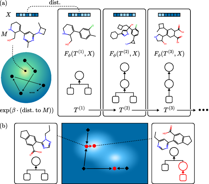
Figure 2: (a) Our Markov Chain Process over the space of syntax trees $\mathcal{T}$. Our Metropolis-Hastings algorithm in Section 3.3 iteratively refines the syntax tree skeleton towards the stationary distribution which is proportional to the inverse distance to $M$, our target molecule. (b) Our genetic algorithm over the joint design space $\mathcal{X}\times\mathcal{T}$ in Section 3.4 combines the strategies of semantic evolution ($\rightarrow$) and syntactical mutation (${\color[rgb]{1,0,0}\rightarrow}$) to encourage both global improvement and local exploration.

3.3 Bilevel Syntax-Semantic Synthesizable Analog Generation

We propose a multi-step factorization to synthesize a program given a molecule $M\in\mathcal{M}$ by first choosing the syntactical skeleton of the solution, then filling in the specific operations and literals. Following the terminology of Section 2.4, we aim to parameterize the derivation procedure of the context-free grammar $G_{\mathcal{P}}$. We define the grammar $G_{\mathcal{P}}$ explicitly and discuss how our syntax-guided approach constrains the grammar in App D. In the following sections, we introduce the main ideas for how we parameterize the derivation of the syntax-guided grammar when conditioned on an input molecule $M$.

The first step $Q\colon\mathcal{M}\rightarrow\mathcal{T}$, where $\mathcal{T}$ is the space of all non-trivial binary trees, is a policy to choose which production rule to apply first. In other words, it recognizes the most likely syntax tree of $P$, given an input $M$. We parameterize $Q_{\Theta}\colon\mathcal{M}\rightarrow\mathcal{T}_{k}$ with a standard MLP for classification. When doing bilevel optimization, this first step is skipped as a sample $T$ is given. The second step is to use $G_{R}\colon\mathcal{T}\times\mathcal{M}\rightarrow\mathcal{P}$ to fill in the reactions. The final step, $G_{B}\colon\mathcal{M}\times\mathcal{P}\rightarrow(P,B)$ produces the final AST, where leaf nodes are literals (building blocks) and non-leaf nodes are operators (reactions). When performing inner-loop only, $F(M)\coloneqq(P_{M;Q},G_{B}(M,P_{M;Q}))$ where $P_{M;Q}\coloneqq G_{R}(Q(M),M)$. However, $Q(M)$ is not necessarily well-defined: there can be multiple skeletons $\{T(;M)\}$ per molecule $M$ (see App B for further investigation). Instead of direct prediction, our outer loop enables systematic exploration over $\mathcal{T}$ via invocation of the inner-loop in a bilevel setup. In this setup, we decouple $T$ from $F$, i.e., $F(M,T)\coloneqq(P_{M},G_{B}(M,P_{M}))$ where $P_{M}\coloneqq G_{R}(T,M)$.

3.3.1 Outer-Loop: Syntax Tree Structure Optimization

We simulate a Markov Process on $\mathcal{T}$, the set of all binary trees for discovering tree structures that maximize similarity between $M$ and the program’s output. The details for how we bootstrap and apply $\mathcal{T}$ is in App A. We adopt the Metropolis-Hastings algorithm with proposal distribution $J(T_{1},T_{2})\propto\exp(-\lambda\cdot\text{dist}(T_{1},T_{2}))$. The scoring function is $\pi(T)\propto\exp(-\beta\cdot\text{dist}(M,\text{exec}(F(M,T))))$ where $\lambda,\beta$ are parameters to tradeoff exploration with exploitation. In other words, we use the inner-loop to score candidates in $\mathcal{T}_{k}$. The optional outer loop benefits from the amortized nature of the inner loop. This highlights how our multi-step factorization decouples the syntactic and semantic components of a complete solution. Next, we discuss our amortized learning strategy for each step.

3.3.2 Inner-loop: Inference of Tree Semantics

We formulate the conditional derivation of $G_{\mathcal{P}}$ after the syntax tree is fixed as a finite horizon Markov decision process (MDP). To bridge $\mathcal{T}$ and $\mathcal{P}$, we introduce an intermediate space of partial programs $\mathcal{T^{\prime}}$. $\mathcal{T^{\prime}}$ consists of all possible partial programs that arise from the following modifications to a $T\in\mathcal{T}$:

1. Prepend a new root node as the parent of the root node of $T$.

2. For the root node, attribute it with any $x\in\mathcal{X}$.

3. Attribute a subset of $T$ with reactions from $\mathcal{R}$.

4. For each leaf node of $T$, attach a left child, and optionally attach a right child.

5. For the newly attached leaf nodes, attribute a subset of them with building blocks from $\mathcal{B}$.

Intuitively, $\mathcal{T}^{\prime}$ is the space of all partially filled in trees in $\mathcal{T}$, with the caveats of adding a root node attributed with a fingerprint describing a hypothetical molecule and adding leaf nodes representing building blocks.

State Space: The state space $S\subset\mathcal{T^{\prime}}$ is the set of all partially filled in trees satisfying topological order, i.e., $S=\{T\in\mathcal{T^{\prime}}\mid\text{$n$ is filled}\Rightarrow\text{parent($n$) is filled, for all }n\in T\}$.

Action Space: The actions $A_{s}$ for a given state available are to fill in a frontier node, i.e., $\{n\in T\mid\text{parent($n$) is filled}\}$ with a reaction from $\mathcal{R}$ if $n$ is a reaction and a building block from $\mathcal{B}$ otherwise.

Policy Network: We parameterize policy networks $G_{R;\Phi}\colon\mathcal{T^{\prime}}\rightarrow\mathcal{R^{*}}$ and $G_{B;\Omega}\colon\mathcal{T^{\prime}}\rightarrow\mathcal{B^{*}}$ by separate graph neural networks, both taking as input a partial program $T^{\prime}$. The network $G_{R;\Phi}$ predicts reactions at the unfilled reaction nodes of $T^{\prime}$, while $G_{B;\Omega}$ predicts embeddings at the unfilled leaf nodes. Since $|\mathcal{B}|\gg|\mathcal{R}|$, $G_{B;\Omega}$ instead predicts 256-dimensional continuous embeddings, from which we retrieve the building block whose 256-dimensional Morgan fingerprint is closest.

Training: We train $\Phi,\Omega$ using supervised policy learning. The key to this approach is the dataset used for training, $D_{\text{pretrain}}$. We construct $D_{\text{pretrain}}$ as follows:

For each (program $P^{(i)}$, building blocks $B^{(i)}$, molecule $M^{(i)}$) in our synthetic dataset,

1. Construct $T^{\prime(i)}$ by prepending a new root node attributed with the fingerprint of $M^{(i)}$ and attaching leaf nodes $L$ corresponding to $B^{(i)}$.

2. For each $\texttt{mask}\in\{0,1\}^{|T^{\prime(i)}|}$ such that $\texttt{mask}[\text{root}(T^{\prime(i)})]$ and $\texttt{mask}[i]\Rightarrow\texttt{mask}[\text{parent}(i)]$ for all $i\in T^{\prime(i)}\setminus\{\text{root}(T^{\prime(i)})\}$,

   1. Obtain the frontier nodes $\text{Fr}_{\texttt{mask}}\leftarrow\{n\in T^{\prime(i)}\mid\texttt{!mask}[n]\cap\texttt{mask}[\mathrm{parent}(n)]\}$

   2. Initialize $(X^{(i)},y^{(i)})$ with all the node features and labels

   3. Mask out $y^{(i)}$ where $n\notin\text{Fr}_{\texttt{mask}}$ and mask out $X^{(i)}$ where $\texttt{!mask}[n]$

   4. Update $D_{\text{pretrain}}\leftarrow D_{\text{pretrain}}\cup\{(T^{\prime(i)},X^{(i)},y^{(i)})\}$

Additional details are in App E.

Decoding: Our decoding algorithm is designed to align with the pretraining strategy, shown in Figure 3. Instead of performing search over an indefinite horizon, we restrict the set of horizon structures to $\mathcal{T}_{k}$, i.e., those present in $D_{\text{pretrain}}$. At test time, we either: (a) use $Q_{\Theta}$ to recognize $T\in\mathcal{T}_{k}$ and initialize the decoding process, or (b) use the algorithm described in Section 3.3.1 to simulate a Markov Chain over $\mathcal{T}_{k}$ and refine the skeleton over time.

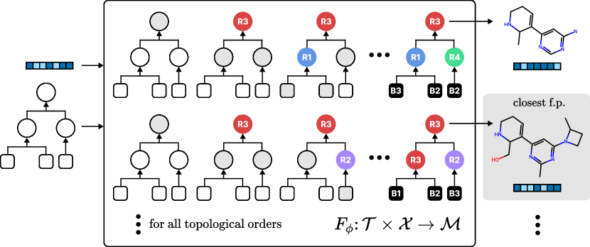
Figure 3: Illustration of our decoding scheme $F_{\phi}(M)$: (Left) The input is a syntax skeleton $T$ and Morgan fingerprint $X$; (Middle) Decode once for every topological ordering of the tree, tracking all partial programs with a stack; (Right) Execute all decoded programs, then returning the closest analog which minimizes distance to $M$.

3.4 Bilevel Syntax-Semantic Synthesizable Molecular Design

The task of synthesizable molecule design is to solve $\operatorname*{arg\,min}_{(P,B)\in\mathcal{P}\times 2^{\mathcal{B}}}f(P(B))$ for a property oracle $f$ of interest. Given the learned parameters from synthetic planning $\Phi,\Omega$, we apply the inner-loop procedure $F_{\Phi,\Omega}(M,T)\colon\mathcal{X}\times\mathcal{T}_{k}\rightarrow\mathcal{P}\times 2^{\mathcal{B}}$ as a surrogate, casting the problem as $\operatorname*{arg\,min}_{(X,T)\in\mathcal{X}\times\mathcal{T}_{k}}f(\text{exec}(F_{\Phi,\Omega}(X,T)))$. This two-step factorization of the design space enables joint optimization over both the semantics and syntax of a solution.

We approach this problem with a Genetic Algorithm (GA) over the joint design space $\mathcal{X}$ and $\mathcal{T}_{k}$. The seed population is obtained by sampling random bit vectors and using $Q_{\Theta}$ to obtain their corresponding skeletons. To generate children $(X,T)$ from two parents $(X_{1},T_{1})$ and $(X_{2},T_{2})$, we combine semantic crossover with syntactical mutation, consistent with our bilevel approach for analog generation:

Semantic Evolution: We generate $X$ by combining bits from both $X_{1}$ and $X_{2}$ and possibly mutating a small number of bits of the crossover result. We then set $T=Q_{\Theta}(X)$.

Syntactic Mutation: We set $X=X_{1}$ and apply edit(s) to $T_{1}$ to obtain $T^{\prime}$. We set $T\leftarrow\text{select}(T^{\prime},T_{1})$ with the selection criteria determined by an exploration-exploitation annealing schedule.

Intuitively, Semantic Evolution optimizes for chemical semantics by combining existing ones from the mating pool, while Syntactic Mutation explores syntactic analogs of specific individuals of interest. Notably, our implementation borrows ideas from simulated annealing [34] to facilitate global diversity during the early iterations of GA and local exploitation during the later iterations of GA. Offspring are generated through a combination of both strategies. Each child is then decoded into a SMILES string using the surrogate and given a fitness score under the property oracle. We then reassign the children’s fingerprints after decoding, i.e., $X\leftarrow\text{FP}(\text{exec}(F_{\Phi,\Omega}(X,T))))$ to reflect our analog exploration strategy. The top scoring unique individuals between are retained into the next generation (i.e., elitist selection). Further details and hyperparameters are given in App F.

4 Experiments

4.1 Experiment Setup

4.1.1 Data Generation

We use 91 reaction templates from [27, 6] representative of common synthetic reactions. They consist primarily of ring formation and fusing reactions but also peripheral modifications. We use 147,505 purchaseable building blocks from Enamine Building Blocks. We follow the same steps as [21] to generate 600,000 synthetic trees. After filtering by QED, we obtain 227,808 synthetic trees (136,684 for training, 45,563 for validation, and 45,561 for test). We then pre-process these trees into programs, constructing our dataset $D_{\text{train}},D_{\text{valid}}$ and $D_{\text{test}}$. We bootstrap our set of syntactic templates, $\hat{\mathcal{T}}$ based on those observed in $D_{\text{train}}$, resulting in 1117 syntactic skeleton classes. Additional statistics on $\hat{\mathcal{T}}$ and insights on its coverage are given in App A.

4.1.2 Baselines

We evaluate against all 25 molecular optimization methods benchmarked in the large-scale experimental study [22]. These methods are divided into three categories, based on the molecule representation: string, graph, or synthetic trees. Synthesis methods restricts the design space to only products of robust template-based reactions, so for fair comparison, so we also report intra-category rankings. We also report the SA Score [18] of the optimized molecules for all methods, both to cross-verify the synthesizability of synthesis-based methods and to investigate the performance trade-off imposed by constraining for template-compatible synthesizability.

4.1.3 Evaluation Metrics

Synthesizable Analog Generation: We evaluate the ability to generate a diverse set of structural analogs to a given input molecule using Average Similarity (as measured by Tanimoto distance to the input) and Internal Diversity (average pairwise Tanimoto distance). We also include the Recovery Rate (RR), whether the most similar analog reconstructs the target, and SA Score [18] as a commonly-used heuristic for synthetic accessibility.

Synthesizable Molecule Design: We evaluate the ability to optimize against calls to 15 Oracle functions [29] relevant to real-world drug discovery. In addition to Top-k average score, we particularly focus on sample efficiency (Top k AUC), as described in [22]. We now describe the different Oracle categories:

1. Bioactivity predictors (GSK3$\beta$/JNK3/DRD2): These estimate responses against targets related to pathogenesis of various diseases such as Alzheimer’s disease [35] using the basis of experimental data [58], and whose inhibitors are the basis for many antipsychotics and have shown promise for treating diseases like Parkinson’s schizophrenia and bipolar disorder [42].

2. Structural profiles (Median1/Median2/Rediscovery): These primarily focus on maximizing structural similarity to multiple molecules, useful for designing molecules fitting a more multifaceted structural profile [4]. The rediscovery oracle focuses on hit expansion around a specific drug.

3. Multi-property objectives (Osimertinib & 6 others): These use real drugs as a basis for optimizing additional pharmacological properties, mimicking how real-world drug discovery works.

4. Docking Simulations ($M^{\text{pro}}$, DRD3): We also add two Docking simulation Oracles against $M^{\text{pro}}$, the main protease of SARS-Cov-2 and DRD3, which has its own leaderboard, with a particular focus on sample efficiency.

Table 1: We generate 5 unique analog molecules conditioned on an input molecule $M$ and sort them by decreasing similarity to $M$. For SynNet, we follow their beam search strategy and produce analogs using the top 5 beams. For Ours (Skeleton), we sample the top 5 syntactic templates from $Q_{\Theta}$. Then, we evaluate how similar, diverse, and structurally simple the first $k$ molecules are. The best method is bolded. For ChEMBL, the second best method is underlined.

Dataset	Method	RR $\uparrow$	Avg. Sim. $\uparrow$			SA Score $\downarrow$			Diversity $\uparrow$
			$k=1$	$k=3$	$k=5$	$k=1$	$k=3$	$k=5$	$k=3$	$k=5$
Test Set	SynNet	46.3%	0.766,	0.622,	0.566	3.108,	3.057,	3.035	0.525,	0.584
	Ours (Skeleton)	52.3%	0.799,	0.588,	0.548	3.075,	2.895,	2.856	0.609,	0.653
ChEMBL	SynNet	4.9%	0.499,	0.436,	0.394	2.669,	2.685,	2.697	0.644,	0.693
	Ours (Skeleton)	7.6%	0.531,	0.443,	0.396	2.544,	2.510,	2.460	0.675,	0.727
	Ours (MCMC)	9.2%	0.532,	0.486,	0.432	2.364,	2.310,	2.263	0.765,	0.759

4.2 Results

4.2.1 Synthesizable Analog Generation

In Table 1, we see our method outperforming SynNet across both dimensions of similarity (how “analog” compounds are) and diversity (how different the compounds are). Additionally, our method achieves lower SA Score, which is a proxy for synthetic accessibility that rewards simpler molecules. Guided by a set of simple yet expressive syntactic templates, our model simultaneously produces more diverse and structurally simple molecules without sacrificing one for the other. Additionally, our policy network is well-suited to navigate these simple yet horizon structures, enabling a $6\%$ higher reconstruction accuracy after training on the same dataset. Combining these three dimensions, we can conclude our method is the superior one for the task of synthesizable analog generation. To better understand which design choices are responsible for the performance, we provided a comprehensive analysis of the policy network in App E. We begin in App E.3 by elaborating on the main distinction of our method vs existing works, highlight the novelty of our formulation, and motivate an auxiliary training task that takes inspiration from cutting-edge ideas in inductive program synthesis. We then perform several key ablations in App E.4, using concrete examples to highlight success and failure cases. Lastly, we perform a step-by-step walkthrough of our decoding algorithm in App E.6, visualizing the evolution of attention weights to showcase the full-horizon awareness of our surrogate and the dynamic incorporation of new information. These analyses shed insights into why our surrogate works, and points to future extensions to make it even better.

4.2.2 Synthesizable Molecule Design

Table 2: We limit to 10000 Oracle calls, then compute Top $k$ and Top $k$ AUC following the settings of [22]. We also include synthetic accessibility scores [18]. The best method per column is bolded, and the best synthesis-based method is underlined. Each Oracle’s output is normalized to $[0,1]$. We compute the Average across all 13 Oracles here. See App. G for the full results and experiment details.

		Average (13 properties)
		Top 1			Top 10			Top 100
	category	Score	SA	AUC	Score	SA	AUC	Score	SA	AUC
synnet	synthesis	0.603 (9|3)	3.074 (7|4)	0.577 (7|2)	0.578 (9|3)	3.075 (6|4)	0.545 (7|2)	0.527 (10|3)	3.094 (7|4)	0.48 (7|2)
pasithea	string	0.418 (24|10)	3.783 (15|7)	0.404 (23|9)	0.338 (24|10)	3.66 (12|5)	0.326 (24|10)	0.249 (24|10)	3.835 (13|6)	0.24 (24|10)
dog_ae	synthesis	0.508 (17|4)	2.845 (4|3)	0.501 (14|4)	0.46 (18|4)	2.857 (3|3)	0.45 (14|4)	0.353 (19|4)	2.809 (3|3)	0.339 (16|4)
smiles_vae_bo	string	0.486 (21|9)	3.18 (8|2)	0.456 (20|8)	0.422 (21|9)	3.084 (7|2)	0.376 (21|8)	0.323 (20|8)	3.055 (4|1)	0.284 (20|8)
jt_vae_bo	graph	0.469 (22|7)	3.571 (11|1)	0.453 (21|7)	0.388 (23|8)	3.5 (10|1)	0.371 (22|8)	0.293 (23|8)	3.559 (10|1)	0.278 (23|8)
moldqn	graph	0.238 (26|10)	5.4 (25|10)	0.209 (26|10)	0.213 (26|10)	5.604 (25|10)	0.187 (26|10)	0.177 (26|10)	5.69 (25|10)	0.151 (26|10)
mars	graph	0.539 (15|5)	4.148 (21|8)	0.508 (13|4)	0.507 (14|5)	4.232 (21|8)	0.47 (12|4)	0.463 (14|5)	4.436 (22|9)	0.41 (13|5)
selfies_lstm_hc	string	0.579 (11|5)	3.617 (12|5)	0.49 (16|6)	0.539 (12|6)	3.743 (14|6)	0.431 (16|6)	0.485 (13|6)	3.82 (12|5)	0.351 (15|6)
gp_bo	graph	0.662 (7|2)	3.981 (18|5)	0.599 (5|2)	0.642 (6|2)	3.954 (16|3)	0.57 (5|2)	0.617 (6|2)	4.054 (17|4)	0.524 (6|2)
smiles_ga	string	0.555 (12|6)	5.107 (23|8)	0.519 (11|5)	0.548 (11|5)	5.422 (23|8)	0.503 (10|5)	0.537 (9|5)	5.578 (23|8)	0.479 (8|4)
mimosa	graph	0.551 (13|4)	4.17 (22|9)	0.499 (15|5)	0.538 (13|4)	4.3 (22|9)	0.463 (13|5)	0.515 (12|4)	4.378 (21|8)	0.417 (12|4)
reinvent	string	0.711 (2|1)	3.352 (9|3)	0.633 (2|1)	0.697 (2|1)	3.415 (9|3)	0.607 (2|1)	0.685 (1|1)	3.48 (9|3)	0.573 (1|1)
smiles_lstm_hc	string	0.695 (3|2)	3.016 (5|1)	0.599 (5|3)	0.667 (5|3)	3.036 (5|1)	0.544 (8|4)	0.622 (5|3)	3.055 (4|1)	0.462 (9|5)
selfies_vae_bo	string	0.502 (18|7)	3.423 (10|4)	0.465 (17|7)	0.428 (19|8)	3.522 (11|4)	0.383 (19|7)	0.318 (22|9)	3.628 (11|4)	0.281 (22|9)
dog_gen	synthesis	0.663 (6|2)	2.766 (3|2)	0.562 (9|3)	0.634 (7|2)	2.793 (2|2)	0.511 (9|3)	0.591 (8|2)	2.803 (2|2)	0.424 (11|3)
stoned	string	0.613 (8|4)	5.364 (24|9)	0.568 (8|4)	0.609 (8|4)	5.55 (24|9)	0.555 (6|3)	0.599 (7|4)	5.667 (24|9)	0.529 (4|2)
gflownet	graph	0.495 (19|6)	4.069 (19|6)	0.461 (19|6)	0.461 (17|6)	4.05 (19|6)	0.419 (17|6)	0.403 (16|6)	4.17 (19|6)	0.359 (14|6)
reinvent_selfies	string	0.693 (5|3)	3.73 (13|6)	0.608 (4|2)	0.682 (3|2)	3.791 (15|7)	0.578 (4|2)	0.654 (3|2)	3.856 (15|7)	0.528 (5|3)
graph_mcts	graph	0.37 (25|9)	3.745 (14|2)	0.332 (25|9)	0.317 (25|9)	3.732 (13|2)	0.28 (25|9)	0.246 (25|9)	3.849 (14|2)	0.213 (25|9)
dst	graph	0.584 (10|3)	4.125 (20|7)	0.522 (10|3)	0.555 (10|3)	4.146 (20|7)	0.479 (11|3)	0.52 (11|3)	4.29 (20|7)	0.426 (10|3)
selfies_ga	string	0.495 (19|8)	5.693 (26|10)	0.358 (24|10)	0.48 (15|7)	5.709 (26|10)	0.337 (23|9)	0.455 (15|7)	5.861 (26|10)	0.306 (19|7)
gflownet_al	graph	0.463 (23|8)	3.829 (16|3)	0.434 (22|8)	0.417 (22|7)	4.005 (18|5)	0.387 (18|7)	0.354 (18|7)	4.153 (18|5)	0.32 (18|7)
screening	N/A	0.52 (16|2)	3.042 (6|2)	0.464 (18|2)	0.426 (20|2)	3.097 (8|2)	0.377 (20|2)	0.322 (21|2)	3.064 (6|1)	0.284 (20|2)
mol_pal	N/A	0.548 (14|1)	2.64 (2|1)	0.517 (12|1)	0.472 (16|1)	3.018 (4|1)	0.444 (15|1)	0.366 (17|1)	3.105 (8|2)	0.339 (16|1)
graph_ga	graph	0.716 (1|1)	3.835 (17|4)	0.631 (3|1)	0.701 (1|1)	3.982 (17|4)	0.601 (3|1)	0.676 (2|1)	4.018 (16|3)	0.553 (3|1)
Ours	synthesis	0.694 (4|1)	2.601 (1|1)	0.642 (1|1)	0.67 (4|1)	2.739 (1|1)	0.608 (1|1)	0.64 (4|1)	2.713 (1|1)	0.554 (2|1)

Table 3: (Left) AutoDock Vina scores against DRD3 and MPro, limited to 5000 Oracle calls. For ZINC (Screening) we use numbers from TDC’s DRD3 Leaderboard. For SynNet, we report both their paper’s numbers and our reproduced runs. (Right) We report the top 3 binders for MPro for the real-world case study in App. H.

			Top 1			Top 10			Top 100
Method	Target	Oracle Calls	Score	SA	AUC	Score	SA	AUC	Score	SA	AUC
ZINC	DRD3	N/A	12.8	$-$	$-$	12.59	$-$	$-$	12.08	$-$	$-$
Synnet		5000	10.8	2.589	10.092	10.3	2.592	9.547	9.197	2.355	8.374
Synnet (paper)		5000	12.3	2.801	$-$	12.02	$-$	$-$	11.133	$-$	$-$
Ours (top k)		5000	13.7	1.908	12.702	13.01	2.128	11.905	12.126	2.175	10.862
Synnet	MPro	5000	8.3	2.821	8.015	8.09	2.267	7.602	7.46	2.249	6.816
Ours (top k)		5000	9.9	2.267	9.478	9.54	2.595	9.009	9.024	2.498	8.288

Method (#Oracle calls)	1st	2nd	3rd
SynNet (5000)	8.3	8.3	8.2
SynNet (Source: Paper)	10.5	9.3	9.3
Ours (5000)	9.9	9.7	9.7
Ours (10000)	10.8	10.7	10.6

Dataset	Method	RR $\uparrow$	Avg. Sim. $\uparrow$			SA Score $\downarrow$			Diversity $\uparrow$
			$k=1$	$k=3$	$k=5$	$k=1$	$k=3$	$k=5$	$k=3$	$k=5$
Train Set	Ours-reverse (Skeleton)	79.30%	0.923	0.632	0.569	3.072	2.795	2.716	0.615	0.657
	Ours (Skeleton)	88.10%	0.958	0.704	0.626	3.099	2.928	2.852	0.532	0.615
Test Set	SynNet	46.30%	0.766	0.622	0.566	3.108	3.057	3.035	0.525	0.584
	Ours-reverse (Skeleton)	40.80%	0.749	0.548	0.487	2.97	2.743	2.659	0.64	0.685
	Ours (Skeleton)	52.30%	0.799	0.588	0.548	3.075	2.895	2.856	0.609	0.653

	1st	2nd	3rd	$k=10$	$k=100$	Diversity
Ours (edits)	0.88	0.88	0.87	0.86	0.8	0.61
Ours (top k)	0.88	0.88	0.87	0.83	0.74	0.55
Ours (flips)	0.87	0.87	0.86	0.84	0.77	0.49

Oracle	Method	$k=1$	$k=10$	$k=100$	Seeds	All
QED	SynNet	0.948	0.948	0.947	$0.673\pm 0.289$	$0.946\pm 0.001$
	SynNet + BO	0.948	0.944	0.933	$0.622\pm 0.270$	$0.931\pm 0.007$
	Ours (edits)	0.948	0.948	0.947	$0.391\pm 0.252$	$\textbf{0.947}\pm\textbf{0.000}$
GSK3$\beta$	SynNet	0.94	0.907	0.815	$0.050\pm 0.051$	$0.803\pm 0.041$
	SynNet + BO	0.85	0.684	0.471	$0.013\pm 0.024$	$0.447\pm 0.090$
	Ours (edits)	0.98	0.967	0.944	$0.074\pm 0.055$	$\textbf{0.941}\pm\textbf{0.012}$
JNK3	SynNet	0.80	0.758	0.719	$0.032\pm 0.025$	$0.715\pm 0.017$
	SynNet + BO	0.310	0.241	0.143	$0.006\pm 0.012$	$0.134\pm 0.039$
	Ours (edits)	0.88	0.862	0.800	$0.059\pm 0.053$	$\textbf{0.792}\pm\textbf{0.030}$
DRD2	SynNet	1.000	1.000	0.998	$0.007\pm 0.018$	$0.996\pm 0.003$
	SynNet + BO	0.982	0.963	0.722	$0.005\pm 0.018$	$0.672\pm 0.147$
	Ours (edits)	1.000	1.000	1.000	$0.024\pm 0.056$	$\textbf{1.000}\pm\textbf{0.000}$

Table 4: (Top left) Ablation 1: Top-down vs Bottom-up (Ours-reverse) Topological Order Decoding; (Bottom left) Ablation 2: Sibling pool generation strategies (edits: mutate skeleton, top $k$: top $k$ skeletons predicted from $Q_{\Theta}$, flips: don’t consider skeleton, flip random bit in the fingerprint) on JNK3 (Right) Ablation 3: SynNet with BO acquisition over sibling pool, generated via top $k$ beams

In Table 2, we see our method outperforming all synthesis-based methods on average across the 13 TDC Oracles for all considered metrics – average score, SA score, and AUC. Surprisingly, our method stays competitive with the SOTA string and graph methods in terms of Average Score (ranking 4th) but being considerably more sample-efficient at finding the top molecules (ranking 1st for Top 1/10 AUC). We see evidence that a synthesizability-constrained design space does not sacrifice end performance when reaping benefits of enhanced synthetic accessibility and sample efficiency.

The AutoDock Vina scores reflect our method’s strength in real-world ligand design tasks. Our best binders against $M^{\text{pro}}$ in Table 3 are significantly better than nearly all known inhibitors from virtual screening or literature [23, 70] ([70] reports a best score of -8.5). Our best binders against DRD3 also rank us 3rd on the TDC Leaderboard (as of Aug. 2024). We present additional analysis of the best binders for our two Docking targets in App H.

4.3 Ablation Studies

In this section, we analyze findings from 3 carefully designed ablation studies (numbered 1-3 in Table 4) to justify the key design decisions that differentiate our method from the predecessor SynNet as well as other synthesis-based methods that have similar modules. We leave a closer investigation of the structure-property relationship to App B.

4.3.1 Top-down vs Bottom-up Topological Order Decoding

Our syntax tree is decoded top-down once the syntactic skeleton is fixed, but it can be argued a bottom-up decoding aligns better with reality and enables pruning, as done by all baselines that serialize the construction of synthesis trees ([2, 3, 21]) and assume the intermediate product satisfies the Markov property. We argue this formulation is ill-defined for early steps, e.g. the model has to predict the first building block to use given only knowledge of the target molecule. This is extremely difficult with orders of magnitude more building blocks than reactions (in our case, 147505 vs 91). Our method resolves this by reformulating the (Markov) state as partial syntax trees, where holes are reactions and building blocks left to predict. This state captures the horizon structure, so we can learn tailored policies for the fixed horizon. We reintroduce the inductive bias of retrosynthetic analysis to procedural synthesis. Conditioned on the syntax (skeleton), we argue a top-down filling order outperforms bottom-up; it is easier to reason backwards from the specification (target molecule) which reactions lead to the product. One may argue a pure bottom-up construction compensates by pruning reactions that don’t match any current precursors. To weigh how much this compensates, we perform an additional Ablation 1: instead of the MDP enforcing we fill in a skeleton top-down, we fill the skeleton from the bottom-up (i.e. a node can only be filled if its children are filled already). We retrain the model by pretraining on inverted masks, and decode by following every possible “reversed” topological order (i.e. topological order of the skeleton with edges reversed). Ablation 1 results show this cannot reconstruct the training data as well and cannot generalize. Conditioned on a syntactic template, we can conclude top-down decoding constrains the search significantly more, even if not able to prune on-the-fly.

4.3.2 Sibling Generation Strategy in Molecule Design

Our analog generation capability is demonstrated in 4.2.1, but it’s not clear how or why it translates to better performance when used as an offspring generator within molecule optimization. Our surrogate takes as input a fingerprint and outputs multiple synthesizable analogs. A good surrogate should output offspring(s) that balance local neighborhood exploration (this Ablation) with global exploitation (Ablation 3). SynNet does the former by mutating the fingerprint directly, whereas the key insight of our syntax-guided method is to mutate the syntactic skeleton instead. Our method achieves this via editing mutations, but it’s not clear whether this is superior to the top recognition strategy employed for the analog generation task ((Skeleton) in Table 1). Table 4 suggests edit-based mutations are superior to the top recognition strategy used for analog generation and the trivial strategy of ignoring the skeleton and flipping individual bits to obtain siblings. This suggests the sibling pool related by edits to the skeleton is a better way to preserve a locality bias within the GA. The simultaneous increase to population diversity and average scores for $k=10,100$ also suggests the same symbiotic relationship between diversity and similarity in analog generation is also the key enabler to better GA optimization.

4.3.3 Comparison against SynNet with Sibling Generation

Our GA benefits from an inner-loop sibling acquisition within the crossover operation, acquiring the best sibling to expend an Oracle call on. It can be argued this extra mechanism is why our method gets better results and makes for an unfair comparison with SynNet, or that this is a method-agnostic hack to improve GA performance. However, we argue the performance gains of this mechanism is unlocked by our syntactic approach to generating a sibling pool. To prove this, we endow SynNet with a similar mechanism in its crossover operation, where we allow it to generate an offspring pool using the top beams then apply a BO acquisition step on top. However, the results not only didn’t improve, but actually downgraded the performance. We hypothesize the reason is SynNet’s optimization trajectory is not helped, but derailed by the additional variation to its sibling pool, reducing local movements within the output space that a syntactic editing approach naturally preserves.

5 Discussion & Conclusion

We reconceptualize the design of synthesis pathways through the lens of program synthesis. Drawing on ideas from syntax-guided synthesis, we introduce a bilevel framework that decouples the syntactical skeleton of a synthetic tree from its chemical semantics. We propose learning algorithms that amortizes over the search for the correct program semantics by fully utilizing the tree horizon structure imposed by the syntactic template. Our results demonstrate this approach’s advantages across the board on key evaluation metrics of conditional analog generation and showcase the method’s capability on challenging synthesizable de novo design problems. Presented with an more expressive design space $\mathcal{T}\times\mathcal{X}$, our method makes the most of the unique opportunities by decoupling the syntactic dimension to navigate a rich, joint design space. Our empirical results demonstrate our algorithms are a step towards capturing the full modeling potential of this design space.

Our bilevel framework not only integrates design and synthesis into a single workflow, significantly reducing the cycle time of traditional molecule discovery, but also invites experts into the loop. Our framework offers a degree of control over the resources involved in the synthesis process. Notably, syntactic templates give users a degree of control over the amount of resources required to execute synthesis and biases the design space towards simpler solutions, making it particularly promising for autonomous synthesis platforms. Combining our workflow with practical deployment, where resource optimization is critical, is an exciting avenue of work [10]. Our framework lays the foundation for an exciting vision: an interactive system that elicits domain expertise in the form of syntactic templates to expedite the procedural synthesis of new molecules. Similar to how syntax-guided program synthesis are meant to involve a programmer in-the-loop, we want to enable the expert to play a role in guiding the optimization towards better solutions.

Appendix A Syntactic Templates

Syntactic templates form the essential ingredients for syntax-guided synthesis, as they significantly reduce the number of possible programs. In practice, syntactical templates are provided by users who operate with real-world constraints or experts who can help narrow the search space to desirable templates. The exact criteria for selecting templates are problem-dependent. To prove our concept in a more generalizable workflow, we bootstrap our set of syntactic templates $\hat{\mathcal{T^{\prime}}}$ in a data-driven way by obtaining the syntactic templates present in $D_{\text{train}}$. We then simulate real-world constraints by setting $\hat{\mathcal{T^{\prime}}_{k}}\leftarrow\{T^{\prime}\in\hat{\mathcal{T^{\prime}}}\mid\text{$T^{\prime}$ has at most $k$ reactions}\}$ and optimize within the design space $\hat{\mathcal{T^{\prime}}_{k}}$. We tabulate summary statistics in 5 for the number of unique syntactic templates and the number of topological orders. We see that the empirical distribution is biased towards simpler syntactic templates, which reflects real-world constraints and is a key enabler of our amortized approach. We train $(\Theta,\Phi,\Omega)_{k}$ for $k=3,4,5,6$ on $D_{\text{pretrain}}$. For samples in $D_{\text{pretrain}}$ with more than $k>6$ reactions, we snap it to the closest $T^{\prime}\in\hat{\mathcal{T^{\prime}}}$ according to the Tree Edit Distance. We find $k=3$ using full topological decoding (illustration in 2) is best for Synthesizable Analog Generation and $k=4$ with random sampling of the decoding beams is a good compromise between accuracy and efficiency for Synthesizable Molecule Design. We also note that the number of unique templates grows sub-exponentially, and in fact the number of templates for a fixed number of reactions starts diminishing for $k>6$. To make sure this does not cause issues, we ensured there is still sufficient coverage to formulate a Markov Chain on $\hat{\mathcal{T^{\prime}}_{k}}$, which is crucial for our bilevel algorithms. For example, 4 visualizes the empirical proposal distribution $J(T_{1},T_{2}),\forall T_{1},T_{2}\in\hat{\mathcal{T^{\prime}}_{4}}\times\hat{\mathcal{T^{\prime}}_{4}}$. Importantly, key hyperparameters like $\beta$ and $n_{\text{edits}}$ enable control over exploration vs exploitation.

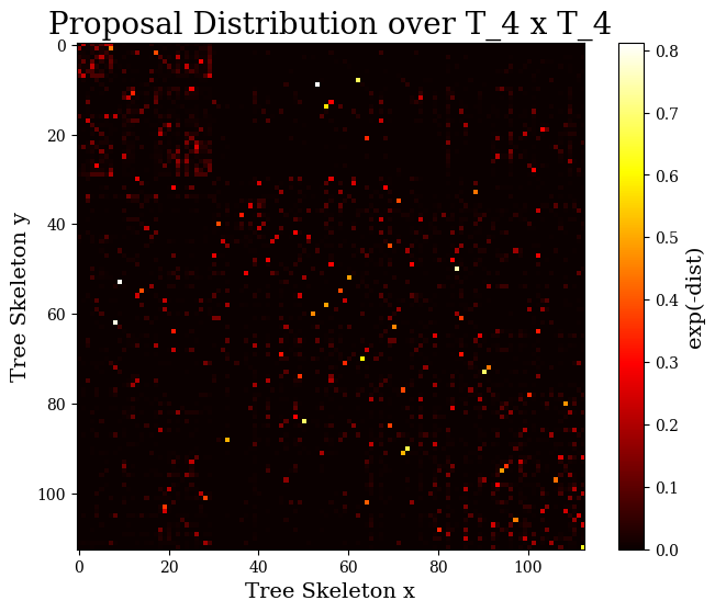
Figure 4: We adopt the Tree Edit Distance as the dist function. We see that $\hat{\mathcal{T^{\prime}}_{4}}$ has sufficient transition coverage for bootstrapping our space of syntactic templates.

No. of Reactions	No. Templates	No. Topological Orders (Max, Mean, Std)
1	2	2, 1.5, 0.5
2	6	8, 4.17, 2.79
3	22	80, 19.59, 20.55
4	83	896, 152.02, 215.53
5	209	19200, 2506.25, 3705.77

(a)

No. of Reactions	No. Templates
6	298
7	243
8	112
9	63
10	42
11	22
12	11
13	4
14	2

(b)

Figure 5: (a) Summary statistics of the number of syntactic templates and possible topological decoding node orders for $k=1,2,\ldots,5$; (b) Summary statistics for only the number of syntactic templates since enumerating all topological sorts becomes intractable

Appendix B Syntax Tree Recognition

In this section, we answer key questions like: (1) How does the relationship change with the addition of $\mathcal{T}$? (2) How strong is the correlation between $\mathcal{X}$ and $\mathcal{T}$? (3) How justified are the most confident predictions made by $Q_{\Theta}$? We investigate the relationship between $\mathcal{M}$ and $\mathcal{T}$. We seek to understand the extent to which the $Q\colon\mathcal{M}\rightarrow\mathcal{T}$ function is well-defined. The first part is quantitative analysis, and the second part is a qualitative study.

B.1 t-SNE and MDS Plots

We use the t-distributed stochastic neighbor embedding (t-SNE) on the final layer hidden representations of our MLP $Q_{\Theta}$ to visualize how our recognition model discriminates between molecules of different syntax tree classes. From 6, we see the MLP is able to discriminate amongst the top 3 or 4 most popular skeleton classes, visually partitioning the representation space. However, beyond that the representations on the validation set begin to coalesce, i.e., the model begins overfitting.

Figure 6: t-SNE on molecules in top (3,4,5,6) skeleton classes

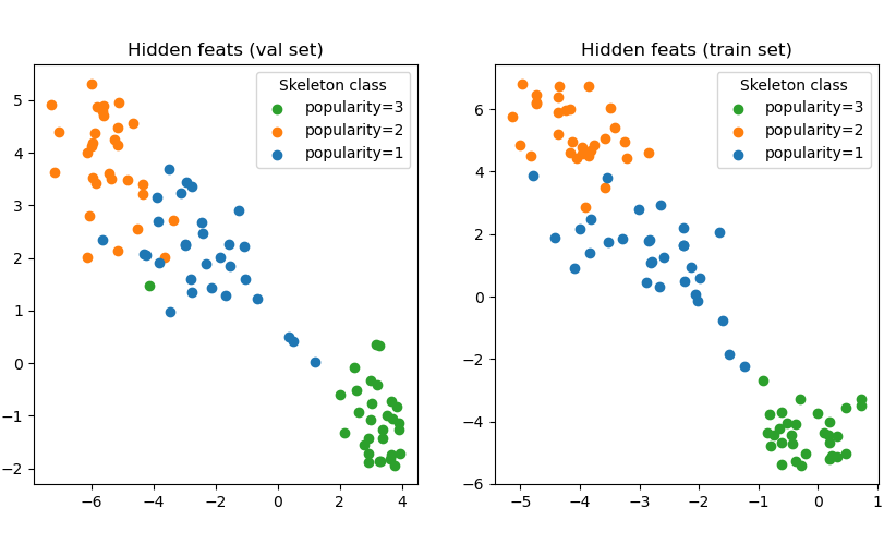
(a) Top 3 (sample 30 each)

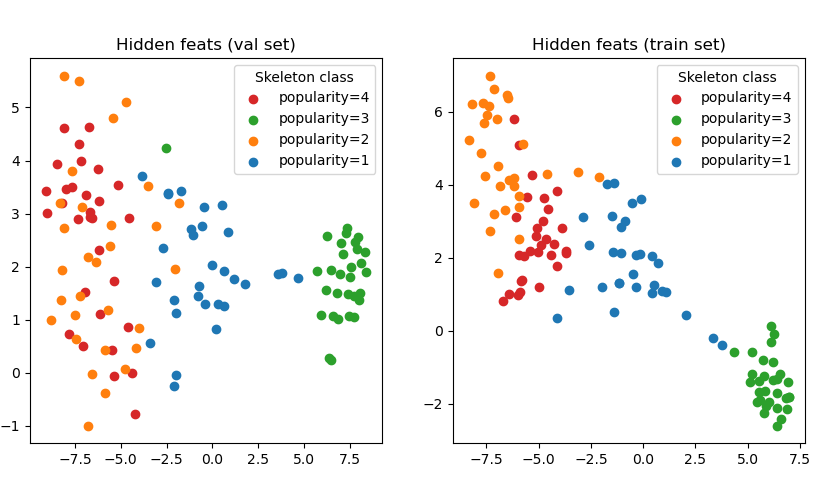
(b) Top 4 (sample 30 each)

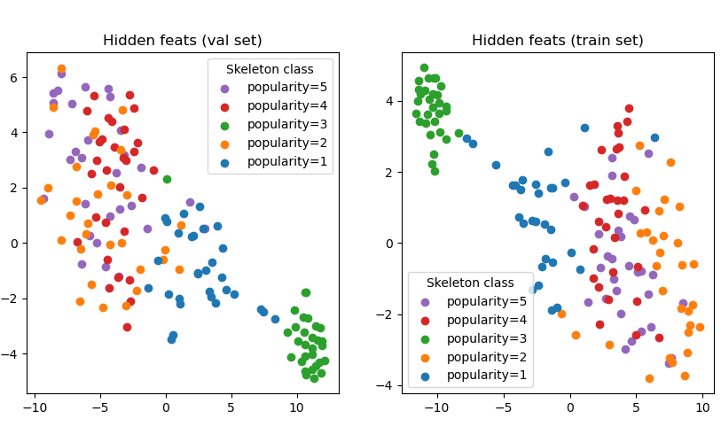
(c) Top 5 (sample 30 each)

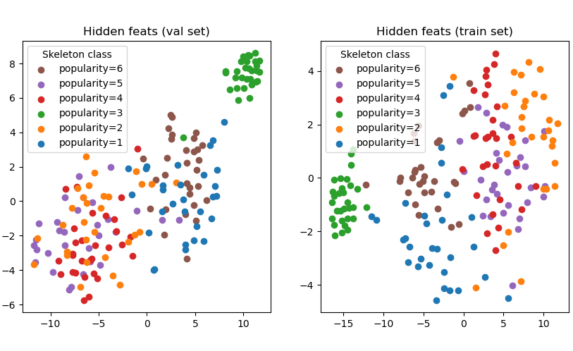
(d) Top 6 (sample 30 each)

Figure 7: MDS on molecules in top (10,20,100) skeleton classes

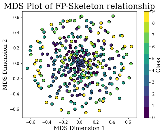
(a) Top 10 (sample 30 each)

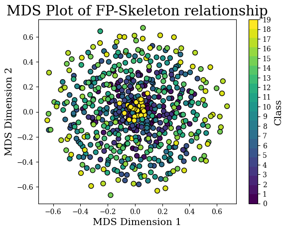
(b) Top 20 (sample 30 each)

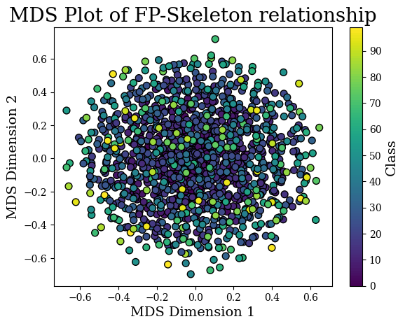
(c) Top 100 (sample 30 each)

Since gradient descent is stochastic, we also use multi-dimensional scaling (MDS) using the Morgan Fingerprint Manhattan distance on a subset of our dataset to visualize the relative positioning between molecules of different syntax tree classes (sorted based on popularity). From the plots in 8, we observe some interesting trends:

• Similarly positioned points tend to have similar colors.

• The darker end of the spectrum corresponding to the most popular classes generally cluster together in the middle.

• The classes do not form disjoint partitions in space. As the ranked popularity increases, the points tend to disperse outwards. There are exception classes, e.g., the yellow set of points in 7(b) that cluster in the center.

Based on these findings, it’s reasonable to conclude a recognition classifier by itself is overly naive. However, the useful inductive bias that similar molecules are more likely to share the same syntactic template indicates the localness property still holds. Our method is designed with this property in mind: we encourage iterative refinement of the syntactic template when doing analog generation.

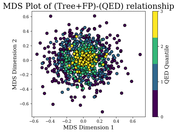
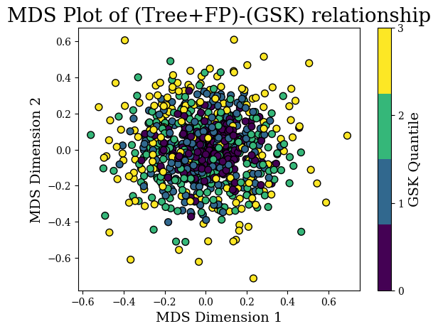
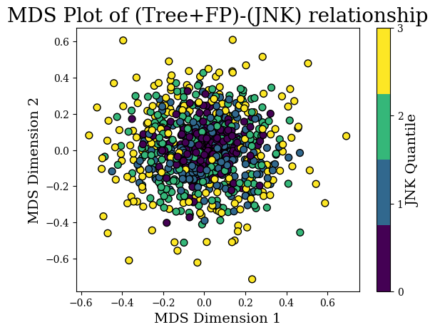
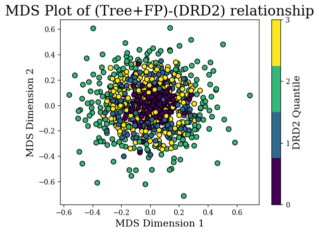
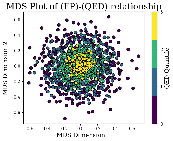
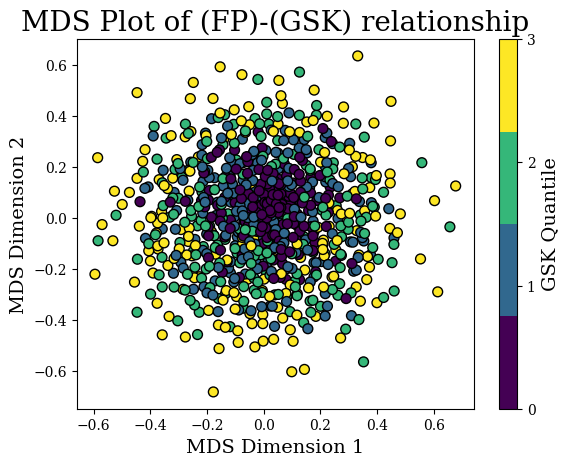
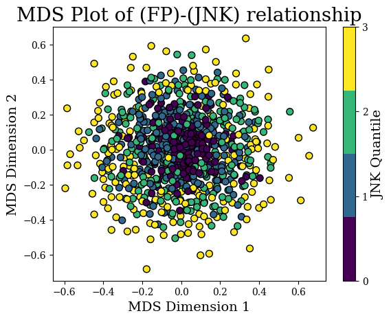
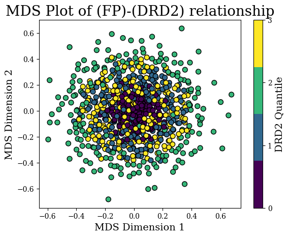
Figure 8: We visualize the structure-property relationship as a scatterplot of 2D structures vs property values. (Top) Structure is $\mathcal{T}\times\mathcal{X}$. We use MDS with the dissimilarity $\text{dist}((T_{1},X_{1}),(T_{2},X_{2}))=\text{Tree-Edit-Distance}(T_{1},T_{2})+\text{Manhattan}(X_{1},X_{2})$. (Bottom) Structure is only $\mathcal{X}$.

We also use MDS to investigate the structure-property relationship to understand the joint effect $\mathcal{T}$ and $\mathcal{X}$ has on different properties of interest. As shown in 8, we see overall, the functional landscape varies significantly from property to property, but the general trend is that decoupling $\mathcal{T}$ from $\mathcal{X}$ does not change the structure-property relationship much. Whereas analog generation requires a more granular understanding of the synergy between $\mathcal{X}$ and $\mathcal{T}$, molecular optimization does not. Instead, the evolutionary strategy should be kept fairly consistent between the original design space $(\mathcal{X})$ and $(\mathcal{X}\times\mathcal{T})$. However, the top row exhibits lower entropy, with the empirical distribution looking “less Gaussian". To capture this nuance, the evolutionary algorithm should combine both global and local optimization steps. We meet this observation with a bilevel optimization strategy that combines Semantic Crossover with Syntactic Mutation.

B.2 Expert Case Study

In this section, we enter the perspective of the recognition model learning the mapping from molecules to syntax tree skeletons. The core difference between this exercise and a common organic chemistry exam question [19] is the option to abstract out the specific chemistry. Since the syntax only determines the skeletal nature of the molecule, the specific low-level dynamics don’t matter. As long as the model can pick up on skeletal similarities between molecules, it will be confident in its prediction. We did the following exercise to understand if cases where the recognition model is most confident on unseen molecules can be attributed to training examples. We took the following steps:

For each true skeleton class $T$

1. Inference the recognition model on 10 random validation set molecules belonging to $T$.

2. Pick the top 2 molecules the model was most confident belongs to $T$.

3. For each molecule $M$.

   1. Find the 2 nearest neighbors to $M$ belonging to $T$ in the training set.

Shown in Figures 9 and 10 is the output of these steps for a common skeleton class which requires two reaction steps.

Figure 9: COc1ncnc(N2C(=O)c3cc([N+](=O)[O-])c(O)cc3N=C2C2NC(=O)OC23CCC3)c1C which recognition model predicts is in its true class with 87.5% probability

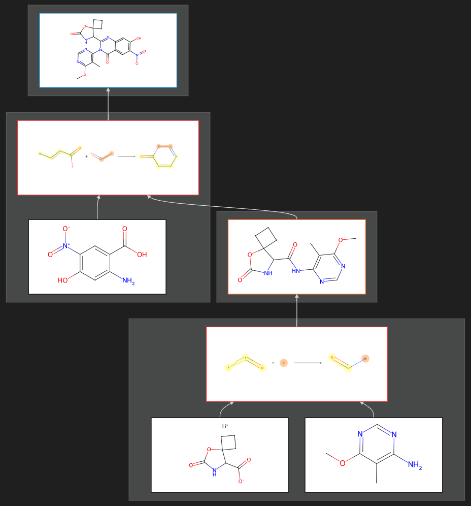
(a) Query molecule

(b) Nearest neighbor in training set

Figure 10: COC(Cc1ccccc1)CN(C1CCCOc2ccccc21)S(=O)(=O)Cc1ccon1 which recognition model predicts is in its true class with 86.2% probability

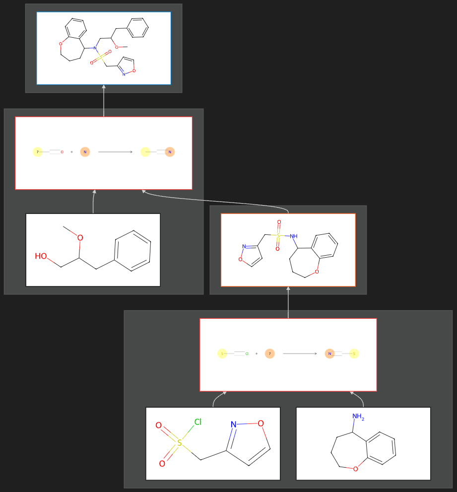
(a) Query molecule

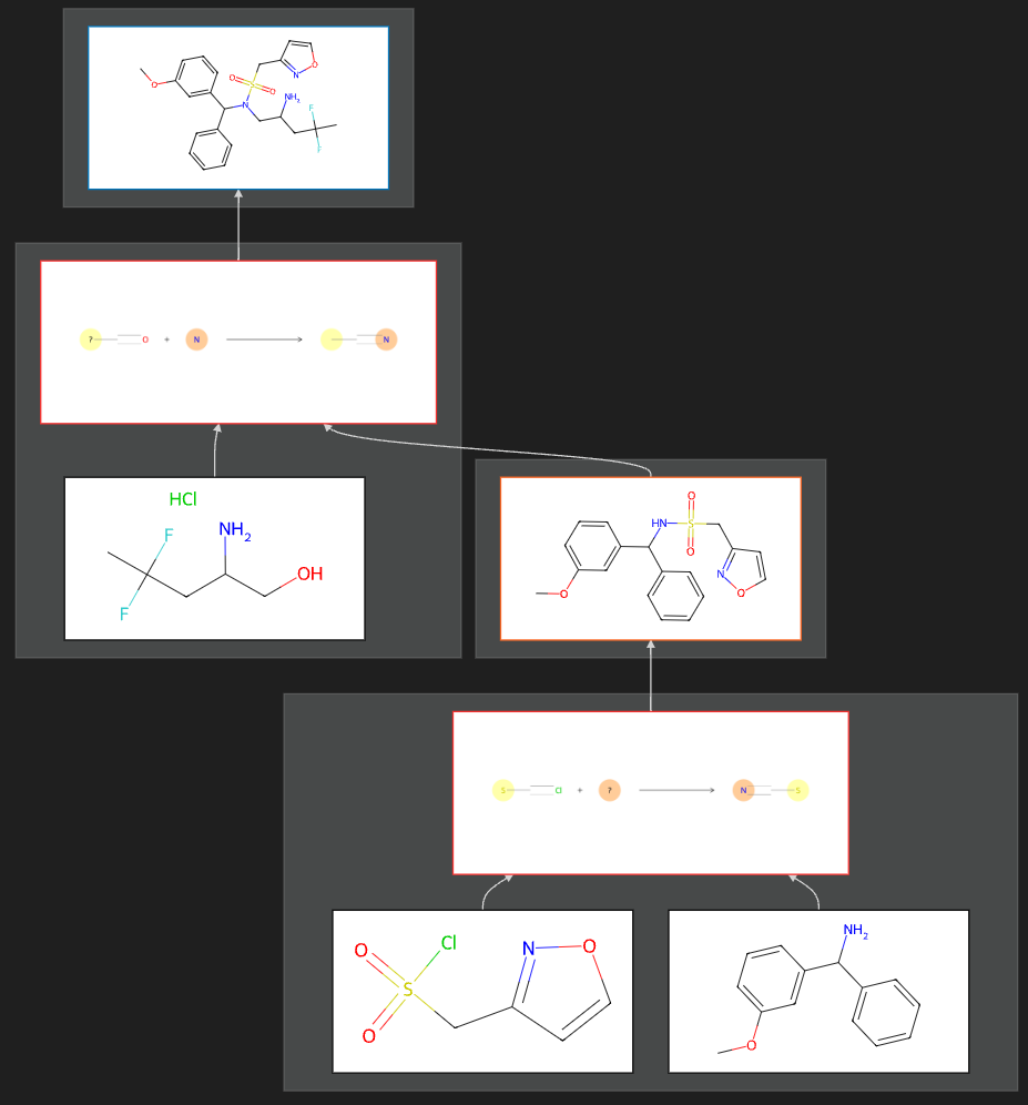
(b) Nearest neighbor in training set

(c) 2nd Nearest neighbor

In Figure 9, we see that the query molecule’s nearest neighbor is an output from the same program but different building blocks. Both feature the same core fused ring system involving a nitrogen. Given that the model has seen 9(b) (and other similar instances), it should associate this core feature with a ring formation reaction step. Taking a step deeper, the respective precursors also share the commonality of having an amide linkage in the middle. Amides are key structural elements that the recognition model can identify. Both precursors underwent the same amide linkage formation step, despite the building blocks being different. Thus, the model’s high confidence on the query molecule can be attributed directly to 9(b).

In Figure 10, there is more “depth" to the matter. We see a skeletal similarity across all three molecules: a nitrogen in the center with three substituents. Although it’s noteworthy that the nitrogen participates in a sulfonamide group in all three cases, using this fact to inform the syntax tree would be a mistake. This is because in 10(a) and 10(b), the sulfonamide group is the result of an explicit sulfonamide formation reaction, where a sulfonyl chloride reacts with an amine. However, in 10(c) the sulfonamide group is already present in a building block. Thus, we see where the recognition model taking as input the circular fingerprint of this molecule could overfit. Nonetheless, the nitrogen with three substituents necessitates at least one reaction is required. The necessity for a second reaction can be attributed to the ether linkage present in both 10(a) and 10(c). The recognizer would be able to justify an additional reaction after it has seen the bicyclic ring structure joined with the sulfonamide group sufficiently many times before. In summary, the model will often be presented multiple complex motifs, but only a subset of them may be responsible for reaction steps. The exact number of reactions needed can only be determined via actually doing the search, but high-level indicators (such as the nitrogen with three substituents) allow the recognition model to abstract out the semantic details and construe a “first guess" of what the syntax tree is.

Appendix C Connection with Program Synthesis

Program synthesis is the problem of synthesizing a function $f$ from a set of primitives and operators to meet some correctness specification. For example, if we want to synthesize a program to find the max of two numbers, the correctness specification $\phi_{\text{max}}\coloneqq f(x,y)\geq x\wedge f(x,y)\geq y\wedge(f(x,y)=x\lor f(x,y)=y)$. As our approach is inspired from ideas in program synthesis, we briefly cover some basic background. A program synthesis problem entails three things:

1. Background theory $\mathsf{T}$ which is the vocabulary for constructing formulas, a typical example being linear integer arithmetic: which has boolean and integer variables, boolean and integer constants, connectives ($\wedge$, $\lor$, $\neg$, $\rightarrow$), operators ($+$), comparisons ($\leq$), conditional (If-Then-Else)

2. Correctness specification: a logical formula involving the output of $f$ and $\mathsf{T}$

3. Set of expressions $L$ that $f$ can take on described by a context-free grammar $G_{L}$.

Program synthesis is often formulated as deducing a constructive proof to the statement: for all inputs, there exists an output such that $\phi$ holds. The constructive proof itself is then the program. At the low-level, program synthesis methods repeatedly calls a SAT solver with the logical formula $\neg\phi$. If UNSAT is returned, this means $f$ is valid. Syntax-guided synthesis [1, 53] (SyGuS) is a framework for meeting the correctness specification with a syntactic template. Syntactic templates explicitly constrains $G_{L}$, significantly reducing the number of implementations $f$ can take on. Sketching is an example application where programmers can sketch the skeletal outline of a program for synthesizers to fill in the rest [57]. More directly related to our problem’s formulation is inductive synthesis, which seeks to generate $f$ to match input/output examples. The problem of synthesis planning for a molecule $M$ is a special case of the programming-by-example paradigm, where we seek to synthesize a program consistent with a single input/output pair: ($\{B\}$, $M$). Inductive synthesis search algorithms have been developed to search through the combinatorial space of derivations of $G_{L}$. In particular, stochastic inductive synthesis use techniques like MCMC to tackle complex synthesis problems where enumerative methods do not scale to. MCMC has been used to optimize for the opcodes in a program [53] or for the Abstract Syntax Tree (AST) directly [1]. In our case, the space of possible program semantics is so large that we decouple the syntax from the semantics, performing stochastic synthesis over only the syntax trees. We also borrow ideas from functional program synthesis, where top-down strategies are preferred over bottom-up ones to better leverage the connection between a high-level specification and a concrete implementation [49]. Similar to how top-down synthesis enables aggressive pruning of the search space via type checking, retrosynthesis algorithms leverages the target molecule $M$ to prune the search space via template compatability checks.

Appendix D Derivation of Grammar

We now define the grammar $G_{\mathcal{P}}$ describing the set of implementations our program can take on. A context-free grammar is a tuple $G_{\mathcal{P}}\coloneqq(\mathcal{N},\Sigma,\mathcal{P},\mathcal{X})$ that contains a set $\mathcal{N}$ of non-terminal symbols, a set $\Sigma$ of terminal symbols, a starting node $\mathcal{X}$, and a set of production rules which define how to expand non-terminal symbols. Recall we are given a set of reaction templates $\mathcal{R}$ and building blocks $\mathcal{B}$. Templates are either uni-molecular ($\coloneqq\mathcal{R}_{1}$) or bi-molecular ($\coloneqq\mathcal{R}_{2}$), such that $\mathcal{R}=\mathcal{R}_{1}\cup\mathcal{R}_{2}$. In the original grammar, these take on the following:

1. Starting symbol: $T$

2. Non-terminal symbols: $R_{1}$, $R_{2}$, $B$

3. Terminal symbols:

   • $\{R\in\mathcal{R}_{1}\}$: Uni-molecular templates

   • $\{R\in\mathcal{R}_{2}\}$: Bi-molecular templates

   • $\{BB\in\mathcal{B}\}$: Building blocks

4. Production rules:

   1. $T\rightarrow R_{1}$

   2. $T\rightarrow R_{2}$

   3. $R_{1}\rightarrow R(B)$ ($\forall R\in\mathcal{R}_{1}$)

   4. $R_{1}\rightarrow R(R_{1})$ ($\forall R\in\mathcal{R}_{1}$)

   5. $R_{1}\rightarrow R(R_{2})$ ($\forall R\in\mathcal{R}_{1}$)

   6. $\forall(X_{1},X_{2})\in\{``R_{1}",``R_{2}",``B"\}\times\{``R_{1}",``R_{2}",``B"\}$

      • $R_{2}\rightarrow R(X_{1},X_{2})$ ($\forall R\in\mathcal{R}_{2}$)

   7. $B\rightarrow BB$ ($\forall BB\in\mathcal{B}$)

Example expressions derived from this grammar are “R3(R3(B1,B2),R2(B3))" and “R4(R1(B2,B1))" for the programs in Figure 1.

Identifying a retrosynthetic pathway can be formulated as the problem of searching through the derivations of this grammar conditioned on a target molecule. This unconstrained approach is extremely costly, since the number of possible derivations can explode.

In our syntax-guided grammar, we are interested in a finite set of syntax trees. The syntax tree of a program depicts how the resulting expression is derived by the grammar. These are either provided by an expert who has to meet experimental constraints, or specified via heuristics (e.g., maximum of $x$ reactions, limiting the tree depth to $y$). For example, the syntax-guided grammar for the set of trees with at most $2$ reactions is specified as follows:

1. Starting symbol: $T$

2. Non-terminal symbols: $R_{1}$, $R_{2}$, $B$

3. Terminal symbols:

   • $\{R\in\mathcal{R}_{1}\}$: Uni-molecular templates

   • $\{R\in\mathcal{R}_{2}\}$: Bi-molecular templates

   • $\{BB\in\mathcal{B}\}$: Building blocks

4. Production rules:

   1. $T\rightarrow R_{2}(B,B)$

   2. $T\rightarrow R_{1}(B)$

   3. $T\rightarrow R_{1}(R_{2}(B,B))$

   4. $T\rightarrow R_{1}(R_{1}(B))$

   5. $T\rightarrow R_{2}(B,R_{1}(B))$

   6. $T\rightarrow R_{2}(B,R_{2}(B,B))$

   7. $T\rightarrow R_{2}(R_{1}(B),B)$

   8. $T\rightarrow R_{2}(R_{2}(B,B),B)$

   9. $R_{1}\rightarrow R$ ($\forall R\in\mathcal{R}_{1}$)

   10. $R_{2}\rightarrow R$ ($\forall R\in\mathcal{R}_{2}$)

   11. $B\rightarrow BB$ ($\forall BB\in\mathcal{B}$)

This significantly reduces the number of possible derivations, but two challenges remain:

• How can when pick the initial production rule when the number of syntax trees grow large? We use an iterative refinement strategy, governed by a Markov Chain Process over the space of syntax trees. The simulation is initialized at the structure predicted from our recognition model B.

• How can we use the inductive bias of retrosynthetic analysis when applying rules 9, 10, 11? We formulate a finite horizon MDP over the space of partial programs, where the actions are restricted to decoding only frontier nodes. This topological order to decoding is consistent with the top-down problem solving done in retrosynthetic analysis. Furthermore, our pretraining and decoding algorithm enumerates all sequences consistent with topological order.

These two questions are addressed by the design choices in 3.3.

Appendix E Policy Network

E.1 Featurization

Recall $\Phi\colon T^{\prime}\rightarrow\mathbb{R}^{|T^{\prime}|\times 91}$ and $\Omega\colon T^{\prime}\rightarrow\mathbb{R}^{|T^{\prime}|\times 256}$. Our dataset $D_{\text{pretrain}}$ consists of instances $(M^{(i)},{T^{\prime}}^{(i)},X^{(i)},y^{(i)})$. We adopt Morgan Fingerprints with radius 2 as our encoder (FP). Then, we featurize each instance as:

$$X^{(i)}_{n} \coloneqq[\text{FP}_{2048}(M^{(i)});\text{BB}(n);\text{RXN}(n)],\qquad$$

$$y^{(i)}_{n} \coloneqq\text{one\_hot}_{91}(n_{\text{RXN\_ID}})\text{ if $n$ is reaction else }\text{FP}_{256}(n_{\text{SMILES}}).$$

$\text{BB}(n)=\text{FP}_{2048}(n_{\text{SMILES}})$ if $n$ is attributed with a building block from $\mathcal{B}$ or $\textbf{0}_{2048}$ otherwise and $\text{RXN}(n)=\text{one\_hot}_{91}(n_{\text{RXN\_ID}})$ if $n$ is attributed with a reaction from $\mathcal{R}$ or $\textbf{0}_{91}$ otherwise. We featurize each building block in $\mathcal{B}$ with their 256-dimension Morgan Fingerprint.

If $\mathcal{N}(T^{\prime})$ and $\mathcal{E}(T^{\prime})$ denote the node and edge set of $T^{\prime}\in\mathcal{T^{\prime}}$, then we define, for convenience:

$$RXN({T^{\prime}}) :=\{r\in\mathcal{N}(T^{\prime})\mid\exists c,p\in\mathcal{N}(T^{\prime})\text{ s.t. }(r,c)\in\mathcal{E}(T^{\prime})\cap(p,r)\in\mathcal{E}(T^{\prime})\}$$ (1)

$$BB({T^{\prime}}) =\{b\in\mathcal{N}(T^{\prime})\mid\nexists c\text{ s.t. }(b,c)\in\mathcal{E}(T^{\prime})\}.\}$$ (2)

E.2 Loss Function

Each sample $(T^{\prime(i)},X^{(i)},y^{(i)})\in D_{\text{pretrain}}$. The loss can be specified as follows:

$$\mathcal{L}_{D_{\text{pretrain}}}(\Phi) \coloneqq\frac{1}{|D_{\text{pretrain}}|}\sum_{i=1}^{|D_{\text{pretrain}}|}\sum_{n\in RXN(T^{\prime(i)})}\text{CE}(F_{\Phi}(T^{\prime(i)})_{n},y^{(i)}_{n}),$$

$$\mathcal{L}_{D_{\text{pretrain}}}(\Omega) \coloneqq\frac{1}{|D_{\text{pretrain}}|}\sum_{i=1}^{|D_{\text{pretrain}}|}\sum_{n\in BB(T^{\prime(i)})}\text{MSE}(F_{\Omega}(T^{\prime(i)})_{n},y^{(i)}_{n}).$$

CE and MSE denote the standard cross entropy loss and mean squared error loss, respectively.

For evaluation, we define the following accuracy metrics:

$$RXN_{\text{acc}}(\Phi) =\frac{1}{|D_{\text{pretrain}}|}\sum_{i=1}^{|D_{\text{pretrain}}|}\frac{1}{|RXN(T^{\prime(i)})|}\sum_{n\in RXN(T^{\prime(i)})}\mathds{1}[\operatorname*{arg\,max}(F_{\Phi}(T^{\prime(i)})_{n})==\operatorname*{arg\,max}(y^{(i)}_{n})],$$

$$NN_{\text{acc}}(\Omega) =\frac{1}{|D_{\text{pretrain}}|}\sum_{i=1}^{|D_{\text{pretrain}}|}\frac{1}{|NN(T^{\prime(i)})|}\sum_{n\in NN(T^{\prime(i)})}\mathds{1}[\operatorname*{arg\,min}_{B\in\mathcal{B}}\text{dist}(F_{\Omega}(T^{\prime(i)})_{n},\text{FP}_{256}(B))==n_{\text{SMILES}}]$$

where we use the cosine distance.

E.3 Auxiliary Training Task

In 3.3.1, we defined the representation $T^{\prime}$ to be the parse tree of a partial program. However, we omitted an extra step that was used to preprocess $T^{\prime}$ for training.

To motivate this step, we first note the distinction between our program synthesis formulation and other formulations. Retrosynthesis is essentially already guided by the execution state at every step. Each expansion in the search tree executes a deterministic reaction template to obtain the new intermediate molecule. Planners based on single-step models [7], for example, assume the Markov Property by training models to directly predict a template given only the intermediate [63, 64]. In program synthesis, meanwhile, the state space is a set of partial programs with actions corresponding to growing the program. The execution of the program (or verification against the specification) does not happen until a complete program is obtained. In recent years, neural program synthesis methods found using auxiliary information in the form of the execution state of a program can help indirectly inform the search [5, 8, 17] since it gives a sense on what the program can compute so far. This insight does not apply to retrosynthesis, since retrosynthesis already executes on the fly. It also does not apply for the methods introduced in 2.3 that construct a synthetic tree in a bottom-up manner, for the same reason (the only difference is they use forward reaction templates, with a much smaller set of robust reaction templates) to obtain the execution state each step. However, as described in 3.3.1, our approach combines the computational advantages of restricting to a small set of forward reaction templates with the inductive bias of retrosynthetic analysis. Our policy is to predict forward reaction templates in a top-down manner. This formulation is common in top-down program synthesis, where an action corresponds to selecting a hole in the program. Similarly, our execution of the program does not happen until the tree is filled in. However, we leverage the insight that the execution state helps in an innovative way. We add an additional step when preprocessing $D_{\text{pretrain}}$: For each $T^{\prime}$ in $D_{\text{pretrain}}$, for each node $r$ corresponding to a reaction, we add a new node $o_{r}$ corresponding to the intermediate outcome of the reaction. If $RXN_{T^{\prime}}$ is the reaction nodes of $T^{\prime}$ as defined in E.1, we can construct $T^{\prime\prime}$ from $T^{\prime}$ as follows:

$$\mathcal{N}(T^{\prime\prime}) \leftarrow\mathcal{N}(T^{\prime})\cup RXN_{T^{\prime}}$$ (3)

$$\mathcal{E}(T^{\prime\prime}) \leftarrow\mathcal{E}(T^{\prime})\cup\{(\text{parent}(r),o_{r}),(o_{r},r)\forall r\in RXN_{T^{\prime}}\}$$ (4)

Figure 11: Examples of $T^{\prime\prime}$ where prediction targets are the frontier reactions (yellow circles), frontier building blocks (numbered yellow squares) and auxiliary intermediates (un-numbered yellow squares).

Lastly, we attribute each $o_{r}$ with the intermediate obtained from the original synthetic tree, i.e. executing the output of the program rooted at $r$. We featurize $\{y_{o}:=\text{FP}_{256}({o}_{\text{SMILES}})\}$ and add them as additional prediction targets to $D_{\text{pretrain}}$. Examples of $T^{\prime\prime}$ are given in 11.

E.4 Ablation Study

To understand whether the two key design choices for $\mathcal{T^{\prime\prime}}$ are justified, we did two ablations:

1. We use the original description of $\mathcal{T^{\prime}}$ in 3.3.1, i.e. without the auxiliary task.

2. We use $\mathcal{T^{\prime\prime}}$, but without attributing the intermediate nodes (so the set of targets is the same as Ablation 1.)

 

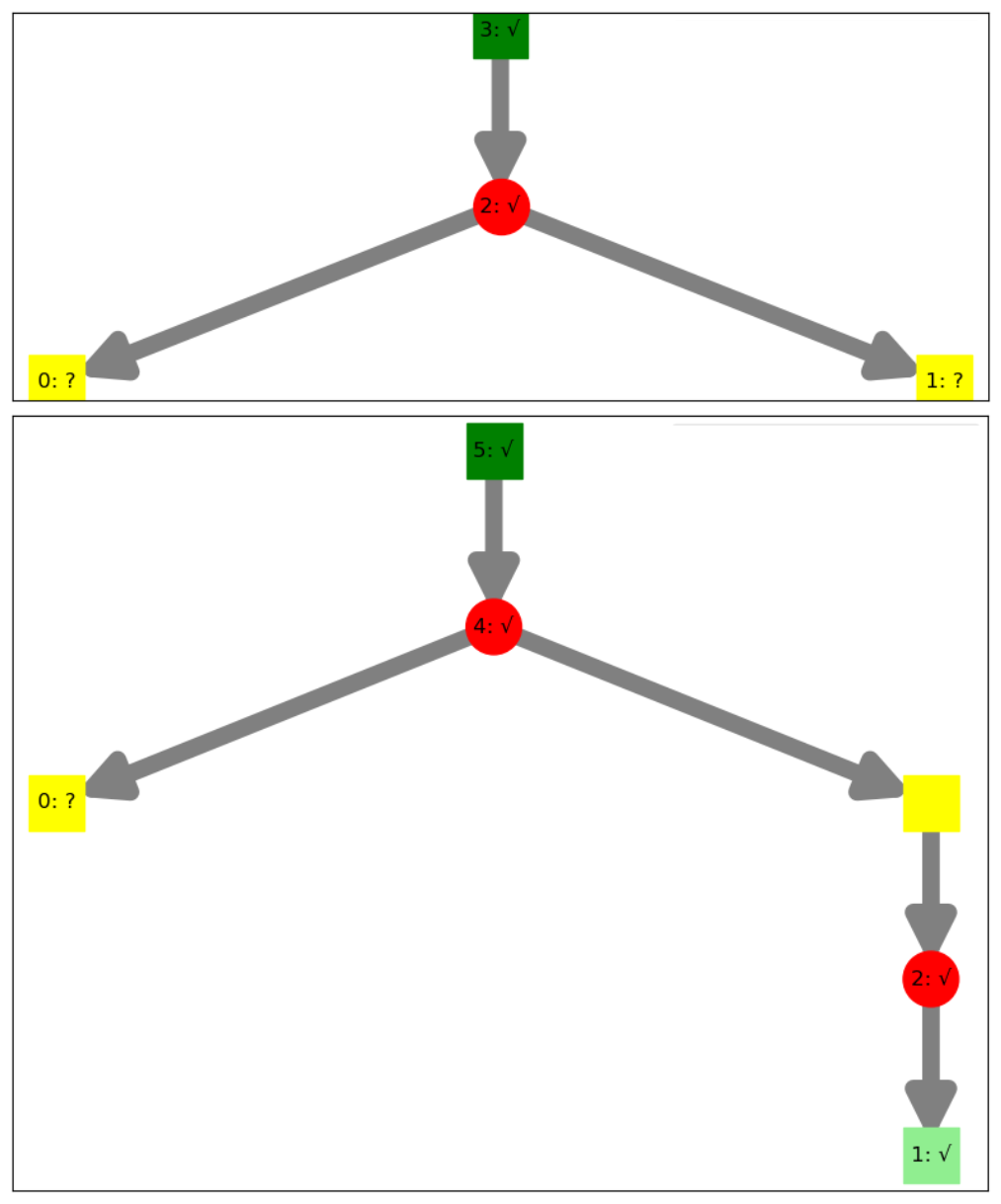
(a) Examples from $\mathcal{T^{\prime\prime}}$

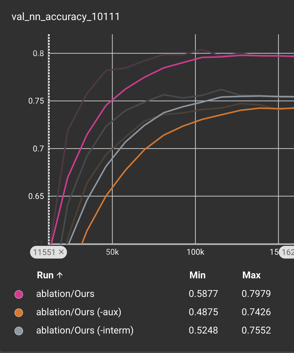
(b) NN accuracy loss over top example 12(a)

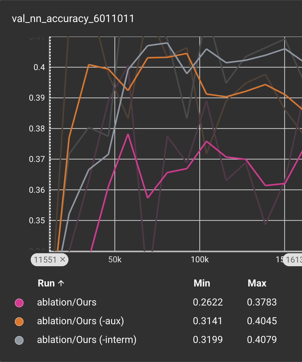
(c) NN accuracy over bottom example 12(a)

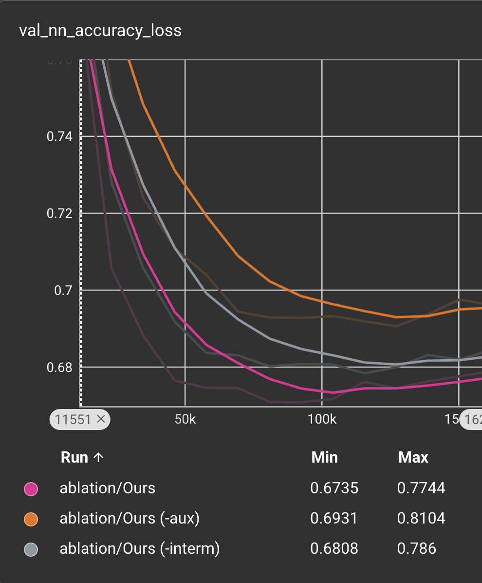
(d) NN accuracy over $D_{\text{valid}}$

Figure 12: We compare the proposed ablations on the NN accuracy metric over the whole dataset as well as on two specific syntactic classes.

As shown in 12(d), using $\mathcal{T^{\prime\prime}}$ (Ours) achieves higher NN accuracy. This shows the benefit of learning the auxiliary training task. Meanwhile, ablating the auxiliary task (-aux) and ablating the intermediate node (-interm) does not have meaningful difference, indicating our architecture is robust to graph edits which are semantically equivalent. To understand the comparative advantage vs disadvantage of the auxiliary training task, consider the two examples in 12(a). The first example is equivalent to learning a single-step backward reaction prediction on forward templates. Our model clearly benefits from the auxiliary training task, which provides additional examples for learning the backward reaction steps. However, our model fares worse on predicting the first reactant of the top reaction. This may be due to competing resources. Despite the task being the same (and the set of forward templates are fixed), the model has to allocate sufficient capacity for the auxiliary task, whose output domain is much higher dimensional than $\mathcal{B}$. Ensuring positive transfer from learning the auxiliary task is an interesting extension for future work.

E.5 Model Architecture

We opt for two Graph Neural Networks (for $\Phi,\Omega$), each with 5 modules. Each module uses a TransformerConv layer [54] (we use 8 attention heads), a ReLU activation, and a Dropout layer. We adopt sinusoidal positional embeddings via numbering nodes using the postorder traversal (to preserve the pairwise node relationships for all instances of the same skeleton). Then, we pretrain $\Phi,\Omega$ with $D_{\text{pretrain}}$.

E.6 Attention Visualization

We elucidate how our policy network leverages the full horizon of the MDP to dynamically adjust the propagation of information throughout the decoding process. Since our decoding algorithm decodes once for every topological order of the nodes, the actual attention dynamics can vary significantly. Thus, we show a prototypical decoding order where:

1. All reactions are decoded before building blocks.

2. If decoding a reaction, the reaction node which $F_{\Phi}$ predicts with the highest probability is decoded.

3. If decoding a building block, the node where the embedding from $F_{\Omega}$ has minimal distance to a building block is decoded.

In [54], each TransformerConv layer $l$ produces an attention weight for each edge, $[\alpha^{(l)}_{i,j}]$ where $\sum_{j}\alpha^{(l)}_{i,j}=1$. We average over all layers to obtain the mean attention weight for each directed edge, i.e., we set the thickness of each edge $(i,j)$ in each subfigure of 13 to be proportional $\sum_{l}\alpha^{(l)}_{i,j}$.

Figure 13: Case Study of Attention Flow

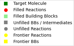
(a) Legend

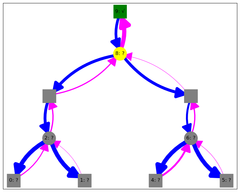
(b) Step 1, decoding candidates: 8

(c) Step 2, decoding candidates: 2, 6

(d) Step 3, decoding candidates: 2

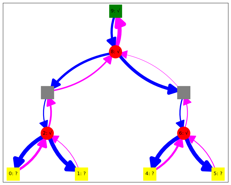
(e) Step 4, decoding candidates: 0, 1, 4, 5

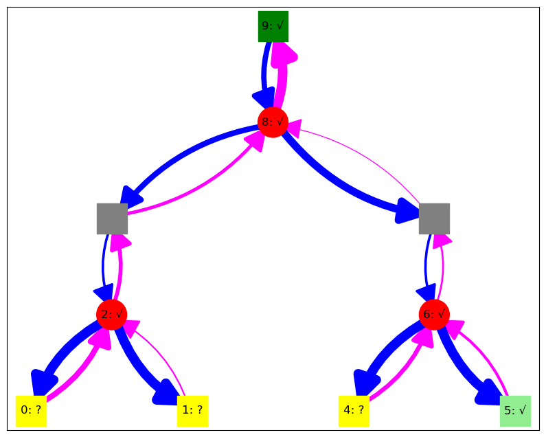
(f) Step 5, decoding candidates: 0, 1, 4

(g) Step 6, decoding candidates: 0, 1

(h) Step 7, decoding candidates: 0

We make some generation observations:

• The information flow along child-parent edges indicate usage of the full horizon. This is the main feature of our approach compared to traditional search methods like retrosynthesis.

• Our positional embeddings enables asymmetric modeling. SMIRKS templates specify the order of reactants and is usually not arbitrary. We observe that more often than not, the parent attends to its left child more than the right child. This may be a consequence of template definition conventions, where the first reactant is the major precursor. The subtree under the node more likely to be the major precursor is more important for predicting the reaction.

Now, we do a detailed walkthrough the 7-step decoding process to understand the evolution of the information flow. Each subfigure corresponds to the state of the MDP after a number of decoding steps, with the candidates of decoding colored in yellow. The attention scores are computed during the inference of $\Phi$ or $\Omega$ and averaged.

1. In 13(b), we see that $8$ attends significantly to the target, unsurprisingly. $8$ also attends to both its children, and attends more to its left child, which is a prior consistent with our general observation.

2. In 13(c), we see that after a specific reaction is instantiated at $8$, the attention dynamics somewhat change. The edge from $8$ to its left child thickens, while the edge from the left child to $8$ thins. This is likely because now that the identity of $8$ is known, it no longer needs to attend to its left child. The reciprocal relationship now intensifies, as the first reactant of $8$ now attends to $8$.

3. In 13(d), after the reaction at $6$ is decoded, we see the information propagate back up the tree and to the other subtree to inform $2$. We see the edge along the path from $6-8$ thickens, indicating the representation of $8$ is informed with new information, and in turn propagates it to $2$.

4. In 13(e), after the reaction at $2$ is decoded, we see the same phenomenon happen, where the information flow again propagates back up and to the other subtree. However, we see this comes with a tradeoff, as $6$ attends to its parent less, and instead reverts to its original attention strength to its children. We hypothesize the identity of $2$ has a strong effect on the posterior of $6$. This is an example where branching out to try more possible orders of decoding would facilitate a more complete algorithm.

5. In 13(f), we see how determining $5$ causes $6$ to attend more to $5$ than it does to its parent. Knowledge of $5$ allows the explaining away of $4$.

6. In 13(g), we note instances of a general phenomenon: the second reactant is decoded followed by the first. Empirically, the distribution of the second reactant has lower entropy than the first. $4$ was inferred after $5$ as the knowledge of its parent reaction and sibling reactant likely constrains its posterior significantly.

7. In 13(h), we see a similar phenomenon where the representation of $2$ attends slightly more to $1$ after it is decoded.

In summary, the syntax structure of the full horizon is crucial during the decoding process. The attention scores allow us to visualize the dynamic propagation of information as nodes are decoded. Our observations highlights the flexibility of this approach compared to an infinite horizon formulation.

Table 5: Hyperparameters of our GA.

	Parameter	Value
General	Max. generations	200
	Population size	128
	Offspring size	512
	Seed initialization	random
	Fingerprint size	2048
	Early stopping warmup	30
	Early stopping patience	10
	Early stopping $\Delta$	0.01
Semantic evolution	Parent selection prob. of $i$	$\propto$ $(\mathrm{rank}(i)+10)$
	Num. crossover bits $n_{\text{cross}}$	$\mathcal{N}(1024,205)$
	Num. mutate bits $n_{\text{flip}}$	12
	Prob. mutate bits $p_{\text{flip}}$	0.5
Syntactic mutation	Parent selection prob. of $i$	$\propto$ $(\mathrm{rank}(i)+10)^{2}$
	Num. tree edits $n_{\text{edit}}$	$\mathcal{U}\{1,2,3\}$
Surrogate	Max. topological orders	5
	Sampling strategy	greedy

Appendix F Genetic Algorithm

Our genetic algorithm (GA) is designed to mimic SynNet’s [21], and settings are given in Table 5. We fix the same number of offspring fitness evaluations per generation to ensure a fair comparison, strategically allocating the evaluations between offspring generated using Semantic Evolution and those generated using Syntactic Mutation.

F.1 Semantic Evolution

Given two parents $(X_{1},T_{1})$ and $(X_{2},T_{2})$, semantic evolution samples a child $(X,T)$ as follows. We obtain $X$ by combining $n_{\text{cross}}$ random bits from $X_{1}$ and the other $2048-n_{\text{cross}}$ bits from $X_{2}$ and then, with probability $p_{\text{flip}}$, flipping $n_{\text{flip}}$ random bits of the crossover result. We set $T=Q_{\Theta}(X)$ using the recognition model.

F.2 Syntactic Mutation

Given an individual $(X,T)$ from F.1, syntactic mutation mutates $T$ to obtain a syntactic analog. We perform $n_{\text{edit}}$ edits on $T$ to obtain $T^{\prime}$. With equal probability, each edit either adds or removes a random leaf. To do so, we enumerate all possible additions and removals, and ignore the ones that produce a mutant tree with less than 2 nodes or more than 4 internal nodes. The edit is uniformly sampled from all such choices, or no operation is performed if no viable choices exist. In the early iterations of the GA, we set $T\leftarrow T^{\prime}$ using the criteria that $\text{exec}(F_{\Phi,\Omega}(X,T^{\prime}))$ promotes a higher Internal Diversity than $\text{exec}(F_{\Phi,\Omega}(X,T))$. In the later iterations of the GA, we use the collected experience of iterations prior to fit a surrogate Gaussian Process. We set $T\leftarrow T^{\prime}$ and accept the mutant if $\text{exec}(F_{\Phi,\Omega}(X,T^{\prime}))$ has higher acquisition value than a counterpart obtained through Semantic Evolution. We refer the reader to work on Particle Swarm Optimization with Gaussian Processes [62, 71, 30] for the related literature.

F.3 Surrogate Checkpoint

The surrogate checkpoint was trained using $D_{\text{pretrain}}$ as described in Appendix E. To lower the runtime of the GA, we only reconstruct using a random subset of the input skeleton’s possible topological orders. For each topological order, we follow a greedy decoding scheme where reactions are decoded before building blocks, as described in Appendix E.6.

Appendix G Full Results on TDC Oracles

Median 1

Median 2

Celecoxib

Top 1

Top 10

Top 100

Top 1

Top 10

Top 100

Top 1

Top 10

Top 100

category

Oracle Calls

Score

SA

AUC

Score

SA

AUC

Score

SA

AUC

Oracle Calls

Score

SA

AUC

Score

SA

AUC

Score

SA

AUC

Oracle Calls

Score

SA

AUC

Score

SA

AUC

Score

SA

AUC

synnet

synthesis

5245

0.245 (15|3)

4.066 (17|4)

0.237 (15|3)

0.228 (13|3)

3.807 (11|3)

0.219 (12|2)

0.198 (14|3)

3.687 (6|3)

0.188 (12|2)

4350.6

0.259 (11|3)

2.364 (5|3)

0.253 (8|2)

0.244 (10|3)

2.473 2|1

0.237 (8|2)

0.214 (11|3)

2.459 (1|1)

0.206 (8|2)

7377.4

0.526 (9|3)

2.234 (14|4)

0.487 (9|3)

0.479 (9|3)

2.262 (7|3)

0.443 (8|3)

0.411 (9|3)

2.466 (12|4)

0.376 (8|3)

pasithea

string

3876.8

0.216 (22|9)

5.432 (26|10)

0.213 (21|8)

0.183 (24|10)

4.486 (23|8)

0.179 (24|10)

0.138 (26|10)

4.319 (18|6)

0.134 (25|10)

2010.8

0.195 (21|9)

2.882 (13|6)

0.194 (21|9)

0.182 (22|9)

2.747 (9|4)

0.181 (20|9)

0.156 (23|9)

2.813 (11|5)

0.154 (23|9)

3901.6

0.355 (22|9)

2.383 (18|7)

0.353 (21|8)

0.317 (21|9)

2.319 (14|4)

0.314 (21|9)

0.247 (23|10)

2.512 (14|5)

0.243 (21|9)

dog_ae

synthesis

1448.4

0.204 (25|4)

3.285 5|1

0.201 (25|4)

0.174 (25|4)

3.192 4|1

0.172 (25|4)

0.139 (24|4)

2.984 (1|1)

0.135 (24|4)

1119.2

0.201 (19|4)

2.347 3|1

0.199 (17|4)

0.185 (20|4)

2.495 (3|2)

0.183 (18|4)

0.16 (22|4)

2.591 (4|3)

0.157 (21|4)

1097.4

0.406 (17|4)

2.23 (13|3)

0.403 (15|4)

0.361 (17|4)

2.278 (10|4)

0.357 (15|4)

0.289 (20|4)

2.395 (7|3)

0.283 (18|4)

smiles_vae_bo

string

10000

0.267 (14|6)

4.307 (20|7)

0.253 (12|6)

0.223 (14|6)

4.244 (20|6)

0.203 (16|6)

0.181 (17|7)

4.252 (14|5)

0.161 (18|7)

10000

0.223 (14|6)

2.759 (10|4)

0.213 (14|6)

0.207 (15|7)

2.608 (5|2)

0.196 (15|7)

0.182 (15|7)

2.626 (6|2)

0.17 (15|7)

10000

0.425 (14|5)

2.225 (12|4)

0.409 (14|5)

0.382 (15|6)

2.312 (13|3)

0.355 (16|6)

0.325 (16|7)

2.374 (6|2)

0.293 (16|7)

jt_vae_bo

graph

4706.6

0.212 (23|9)

5.21 (25|10)

0.21 (22|9)

0.184 (23|9)

4.187 (17|9)

0.18 (22|9)

0.151 (23|9)

4.052 (10|4)

0.145 (22|8)

5246.8

0.193 (22|7)

3.013 (14|3)

0.192 (22|7)

0.183 (21|7)

3.125 (17|4)

0.181 (20|6)

0.165 (21|8)

3.196 (16|3)

0.16 (18|6)

4538

0.39 (20|7)

2.408 (20|7)

0.387 (19|6)

0.306 (22|7)

2.496 (18|6)

0.3 (22|7)

0.25 (22|7)

2.744 (19|6)

0.241 (22|7)

moldqn

graph

10000

0.188 (26|10)

4.654 (23|9)

0.144 (26|10)

0.169 (26|10)

4.972 (25|10)

0.123 (26|10)

0.139 (24|10)

5.387 (25|10)

0.094 (26|10)

10000

0.109 (26|10)

5.837 (26|10)

0.095 (26|10)

0.1 (26|10)

5.666 (26|10)

0.089 (26|10)

0.085 (26|10)

5.554 (26|10)

0.072 (26|10)

10000

0.128 (26|10)

4.708 (26|10)

0.115 (26|10)

0.112 (26|10)

4.951 (26|10)

0.1 (26|10)

0.094 (26|10)

5.255 (26|10)

0.08 (26|10)

mars

graph

3698.6

0.233 (18|7)

3.823 (15|7)

0.228 (17|6)

0.217 (16|5)

4.063 (14|7)

0.208 (14|5)

0.181 (17|6)

4.13 (11|5)

0.17 (15|5)

4298.2

0.204 (17|4)

3.036 (15|4)

0.197 (18|4)

0.19 (18|5)

3.446 (22|9)

0.182 (19|5)

0.17 (18|6)

3.774 (23|9)

0.16 (18|6)

7404.6

0.487 (11|3)

2.16 (8|4)

0.429 (10|3)

0.448 (10|3)

2.3 (11|4)

0.38 (14|5)

0.394 (11|4)

2.468 (13|3)

0.318 (15|5)

selfies_lstm_hc

string

10000

0.363 (5|4)

3.533 (13|4)

0.269 (10|5)

0.339 (5|4)

3.669 (10|4)

0.24 (10|5)

0.286 (7|4)

3.833 (8|2)

0.201 (10|5)

10000

0.274 (8|4)

2.184 (2|1)

0.229 (12|5)

0.262 (9|5)

2.402 (1|1)

0.207 (12|5)

0.24 (9|5)

2.564 (3|1)

0.179 (13|6)

10000

0.586 (8|4)

2.205 (10|2)

0.427 (11|4)

0.535 (8|4)

2.193 (3|1)

0.387 (11|4)

0.474 (8|4)

2.239 (2|1)

0.326 (14|6)

gp_bo

graph

10000

0.345 (7|2)

4.111 (18|8)

0.317 (5|2)

0.333 (6|1)

3.992 (13|6)

0.302 (4|1)

0.317 (3|1)

4.452 (22|9)

0.276 (3|1)

10000

0.337 (2|1)

3.4 (22|8)

0.31 (1|1)

0.33 (1|1)

3.358 (21|8)

0.298 (1|1)

0.313 (1|1)

3.303 (18|5)

0.276 (1|1)

10000

0.946 (2|1)

2.179 (9|5)

0.809 (1|1)

0.859 (2|1)

2.274 (8|2)

0.725 (1|1)

0.803 (2|1)

2.648 (16|5)

0.638 (2|1)

smiles_ga

string

3093

0.208 (24|10)

4.708 (24|9)

0.205 (23|9)

0.2 (21|8)

5.686 (26|10)

0.192 (20|8)

0.199 (13|6)

5.93 (26|10)

0.186 (13|6)

6634.6

0.211 (15|7)

3.352 (20|8)

0.204 (15|7)

0.208 (14|6)

3.453 (23|8)

0.199 (14|6)

0.204 (12|6)

3.751 (22|8)

0.192 (10|5)

3104.6

0.358 (21|8)

3.378 (24|9)

0.352 (22|9)

0.356 (19|7)

3.801 (24|9)

0.345 (18|7)

0.35 (15|6)

3.999 (24|9)

0.332 (13|5)

mimosa

graph

10000

0.296 (10|3)

3.481 (11|4)

0.271 (9|3)

0.276 (10|3)

3.928 (12|5)

0.244 (9|3)

0.251 (10|3)

4.263 (16|7)

0.213 (8|3)

10000

0.238 (13|3)

2.739 (9|1)

0.228 (13|3)

0.229 (12|3)

2.826 (10|1)

0.215 (10|3)

0.216 (10|3)

3.08 (15|2)

0.196 (9|3)

9260

0.438 (13|5)

3.064 (22|9)

0.422 (13|5)

0.428 (11|4)

3.081 (21|8)

0.395 (10|3)

0.406 (10|3)

3.322 (22|9)

0.355 (10|3)

reinvent

string

6022

0.4 (1|1)

3.353 (6|2)

0.368 (2|1)

0.399 (1|1)

3.415 (6|2)

0.357 (1|1)

0.383 (1|1)

4.032 (9|3)

0.325 (1|1)

10000

0.333 (3|2)

2.475 (7|3)

0.29 (2|1)

0.326 (2|1)

2.661 (7|3)

0.278 (2|1)

0.313 (1|1)

2.737 (10|4)

0.259 (2|1)

6641.8

0.96 (1|1)

2.157 (7|1)

0.803 (2|1)

0.862 (1|1)

2.355 (16|6)

0.715 (2|1)

0.821 (1|1)

2.724 (17|6)

0.647 (1|1)

smiles_lstm_hc

string

10000

0.389 (4|3)

4.199 (19|6)

0.299 (7|3)

0.351 (3|3)

4.299 (21|7)

0.256 (7|4)

0.315 (4|3)

4.243 (13|4)

0.214 (7|4)

10000

0.34 (1|1)

3.266 (18|7)

0.277 (4|2)

0.318 (3|2)

3.026 (15|7)

0.249 (6|3)

0.291 (5|3)

2.682 (8|3)

0.218 (7|4)

10000

0.851 (3|2)

2.22 (11|3)

0.621 (5|2)

0.786 (3|2)

2.311 (12|2)

0.54 (6|3)

0.695 (3|2)

2.403 (9|3)

0.45 (6|3)

selfies_vae_bo

string

10000

0.232 (19|7)

4.539 (22|8)

0.226 (18|7)

0.212 (18|7)

4.612 (24|9)

0.202 (17|7)

0.175 (19|8)

4.45 (21|8)

0.16 (19|8)

10000

0.206 (16|8)

2.45 (6|2)

0.202 (16|8)

0.192 (17|8)

2.896 (13|6)

0.186 (16|8)

0.169 (19|8)

3.065 (14|7)

0.16 (18|8)

10000

0.391 (19|7)

2.366 (17|6)

0.389 (17|6)

0.353 (20|8)

2.323 (15|5)

0.327 (20|8)

0.29 (19|8)

2.446 (10|4)

0.262 (20|8)

dog_gen

synthesis

8862.6

0.323 (8|2)

3.459 (10|3)

0.244 (14|2)

0.296 (8|2)

3.419 (7|2)

0.218 (13|3)

0.261 (9|2)

3.483 (4|2)

0.182 (14|3)

10000

0.297 6|1

2.708 (8|4)

0.23 (11|3)

0.287 6|1

2.571 (4|3)

0.213 (11|3)

0.263 (7|2)

2.511 (2|2)

0.189 (12|3)

9319

0.76 5|1

2.09 (6|2)

0.526 (7|2)

0.682 6|1

2.189 2|1

0.466 (7|2)

0.584 6|1

2.243 (3|2)

0.389 (7|2)

stoned

string

4140.8

0.295 (11|5)

3.911 (16|5)

0.282 (8|4)

0.283 (9|5)

4.236 (19|5)

0.267 (6|3)

0.264 (8|5)

4.782 (24|9)

0.245 (6|3)

9341.8

0.266 (10|5)

3.785 (24|9)

0.25 (9|4)

0.264 (8|4)

3.913 (24|9)

0.246 (7|4)

0.26 (8|4)

4.097 (24|9)

0.237 (5|2)

6255

0.401 (18|6)

3.129 (23|8)

0.389 (17|6)

0.398 (14|5)

3.477 (23|8)

0.383 (12|5)

0.393 (12|5)

3.657 (23|8)

0.368 (9|4)

gflownet

graph

10000

0.237 (17|6)

2.83 (3|3)

0.225 (19|7)

0.217 (16|5)

3.026 (3|3)

0.202 (17|6)

0.187 (15|5)

3.332 (3|2)

0.166 (16|6)

10000

0.198 (20|6)

3.513 (23|9)

0.195 (19|5)

0.189 (19|6)

3.351 (20|7)

0.181 (20|6)

0.175 (17|5)

3.63 (20|7)

0.165 (17|5)

10000

0.409 (16|6)

2.864 (21|8)

0.375 (20|7)

0.36 (18|6)

3.12 (22|9)

0.328 (19|6)

0.308 (18|6)

3.237 (21|8)

0.276 (19|6)

reinvent_selfies

string

4209.2

0.4 (1|1)

3.353 (6|2)

0.368 (2|1)

0.396 (2|2)

3.399 (5|1)

0.356 (2|2)

0.34 (2|2)

3.779 (7|1)

0.3 (2|2)

9729.8

0.313 (5|3)

2.766 (11|5)

0.27 (5|3)

0.31 (5|3)

2.841 (12|5)

0.256 (5|2)

0.301 (3|2)

2.988 (12|6)

0.233 (6|3)

7480.2

0.751 (7|3)

2.283 (15|5)

0.618 (6|3)

0.722 (5|3)

2.568 (19|7)

0.574 (5|2)

0.685 (5|3)

2.725 (18|7)

0.516 (4|2)

graph_mcts

graph

10000

0.243 (16|5)

2.692 (2|2)

0.235 (16|5)

0.212 (18|7)

2.898 (1|1)

0.196 (19|7)

0.164 (21|7)

3.545 (5|3)

0.144 (23|9)

10000

0.149 (25|9)

3.203 (16|5)

0.142 (24|9)

0.14 (25|9)

3.123 (16|3)

0.133 (24|9)

0.128 (25|9)

3.252 (17|4)

0.118 (24|9)

10000

0.329 (24|9)

2.047 (3|1)

0.297 (23|8)

0.296 (23|8)

2.256 (6|1)

0.265 (23|8)

0.233 (25|9)

2.4 (8|1)

0.205 (24|9)

dst

graph

10000

0.281 (12|4)

3.754 (14|6)

0.257 (11|4)

0.263 (11|4)

3.651 (9|4)

0.233 (11|4)

0.231 (11|4)

4.153 (12|6)

0.194 (11|4)

10000

0.202 (18|5)

2.778 (12|2)

0.195 (19|5)

0.195 (16|4)

2.835 (11|2)

0.186 (16|4)

0.178 (16|4)

3.039 (13|1)

0.167 (16|4)

9723.8

0.459 (12|4)

2.082 (5|3)

0.424 (12|4)

0.422 (13|5)

2.277 (9|3)

0.381 (13|4)

0.381 (13|5)

2.446 (10|2)

0.335 (12|4)

selfies_ga

string

8900.6

0.219 (21|8)

2.877 (4|1)

0.202 (24|10)

0.199 (22|9)

3.467 (8|3)

0.18 (22|9)

0.172 (20|9)

4.445 (20|7)

0.153 (20|9)

10000

0.161 (24|10)

5.071 (25|10)

0.129 (25|10)

0.157 (24|10)

5.005 (25|10)

0.122 (25|10)

0.149 (24|10)

4.988 (25|10)

0.111 (25|10)

10000

0.289 (25|10)

3.961 (25|10)

0.242 (25|10)

0.27 (25|10)

4.122 (25|10)

0.224 (25|10)

0.252 (21|9)

4.547 (25|10)

0.2 (25|10)

gflownet_al

graph

10000

0.229 (20|8)

1.877 (1|1)

0.224 (20|8)

0.203 (20|8)

2.933 (2|2)

0.191 (21|8)

0.164 (21|7)

3.262 (2|1)

0.146 (21|7)

10000

0.191 (23|8)

3.269 (19|6)

0.183 (23|8)

0.182 (22|8)

3.338 (18|5)

0.174 (23|8)

0.167 (20|7)

3.717 (21|8)

0.157 (21|8)

10000

0.333 (23|8)

2.4 (19|6)

0.29 (24|9)

0.286 (24|9)

2.686 (20|7)

0.258 (24|9)

0.24 (24|8)

3.018 (20|7)

0.214 (23|8)

screening

N/A

10000

0.272 (13|2)

4.361 (21|2)

0.25 (13|2)

0.223 (14|2)

4.37 (22|2)

0.206 (15|2)

0.182 (16|2)

4.386 (19|1)

0.162 (17|2)

10000

0.245 (12|2)

3.223 (17|2)

0.233 (10|2)

0.213 (13|2)

2.732 (8|1)

0.201 (13|2)

0.184 (14|2)

2.671 (7|2)

0.171 (14|2)

10000

0.419 (15|2)

2.344 (16|2)

0.396 (16|2)

0.373 (16|2)

2.232 (5|2)

0.353 (17|2)

0.317 (17|2)

2.332 (5|2)

0.29 (17|2)

mol_pal

N/A

10000

0.31 (9|1)

3.385 (9|1)

0.302 (6|1)

0.257 (12|1)

4.21 (18|1)

0.25 (8|1)

0.211 (12|1)

4.645 (23|2)

0.203 (9|1)

10000

0.273 (9|1)

2.12 (1|1)

0.267 (7|1)

0.237 (11|1)

2.897 (14|2)

0.232 (9|1)

0.198 (13|1)

2.593 (5|1)

0.192 (10|1)

10000

0.511 (10|1)

1.908 (1|1)

0.498 (8|1)

0.427 (12|1)

2.097 (1|1)

0.416 (9|1)

0.364 (14|1)

2.245 (4|1)

0.351 (11|1)

graph_ga

graph

10000

0.351 (6|1)

3.492 (12|5)

0.32 (4|1)

0.331 (7|2)

4.137 (15|8)

0.295 (5|2)

0.31 (5|2)

4.304 (17|8)

0.265 (4|2)

10000

0.324 (4|2)

3.383 (21|7)

0.289 (3|2)

0.316 (4|2)

3.346 (19|6)

0.274 (3|2)

0.3 (4|2)

3.335 (19|6)

0.252 (3|2)

9685.4

0.811 (4|2)

2.067 (4|2)

0.684 (3|2)

0.757 (4|2)

2.406 (17|5)

0.631 (3|2)

0.693 (4|2)

2.622 (15|4)

0.559 (3|2)

Ours

synthesis

8303

0.4 (1|1)

3.353 (6|2)

0.371 (1|1)

0.342 4|1

4.161 (16|4)

0.305 (3|1)

0.298 6|1

4.256 (15|4)

0.252 (5|1)

9117

0.292 (7|2)

2.353 (4|2)

0.269 (6|1)

0.285 (7|2)

2.649 (6|4)

0.257 (4|1)

0.272 6|1

2.682 (8|4)

0.238 (4|1)

7042

0.753 (6|2)

1.959 2|1

0.662 (4|1)

0.668 (7|2)

2.195 (4|2)

0.582 (4|1)

0.572 (7|2)

2.211 (1|1)

0.503 (5|1)

Table 6: Guacamol structural target-directed benchmarks: Median 1 & 2 (average similarity to multiple molecules) and Celecoxib Rediscovery (hit expansion around Celecoxib).

GSK3$\beta$

JNK3

DRD2

Top 1

Top 10

Top 100

Top 1

Top 10

Top 100

Top 1

Top 10

Top 100

category

Oracle Calls

Score

SA

AUC

Score

SA

AUC

Score

SA

AUC

Oracle Calls

Score

SA

AUC

Score

SA

AUC

Score

SA

AUC

Oracle Calls

Score

SA

AUC

Score

SA

AUC

Score

SA

AUC

synnet

synthesis

9059.4

0.932 (8|3)

2.576 (5|2)

0.855 (6|3)

0.901 (8|3)

2.747 (6|3)

0.79 (6|3)

0.797 (9|3)

2.897 (6|4)

0.656 (7|2)

6240

0.798 (7|3)

2.116 (3|2)

0.723 (3|1)

0.715 (8|3)

2.172 (1|1)

0.631 (5|2)

0.563 (10|3)

2.244 (2|2)

0.466 (9|2)

6472.6

1.0 (1|1)

2.58 (7|3)

0.985 (4|3)

0.998 (9|3)

2.806 (8|4)

0.969 (1|1)

0.986 (12|3)

2.845 (7|4)

0.898 (4|2)

pasithea

string

2531.2

0.414 (24|10)

3.34 (14|5)

0.402 (23|9)

0.294 (25|10)

3.277 (11|3)

0.282 (24|10)

0.151 (26|10)

3.782 (13|4)

0.141 (26|10)

2707.4

0.21 (24|10)

2.804 (9|4)

0.207 (24|10)

0.158 (24|10)

2.669 (9|3)

0.155 (24|10)

0.081 (26|10)

3.433 (13|5)

0.076 (24|10)

2983.2

0.592 (24|10)

4.057 (22|7)

0.559 (23|9)

0.275 (25|10)

3.894 (22|7)

0.256 (25|10)

0.065 (25|10)

3.858 (19|7)

0.06 (25|10)

dog_ae

synthesis

1319

0.778 (12|4)

2.727 (8|4)

0.756 (10|4)

0.624 (14|4)

2.86 (7|4)

0.602 (13|4)

0.378 (18|4)

2.874 (5|3)

0.356 (16|4)

1219.8

0.554 (13|4)

2.38 (6|4)

0.54 (12|4)

0.493 (13|4)

2.625 (7|4)

0.47 (12|4)

0.263 (17|4)

2.734 (8|4)

0.246 (16|4)

1337

0.999 (11|4)

2.444 (5|2)

0.986 (3|2)

0.979 (15|4)

2.495 (4|2)

0.944 (6|4)

0.589 (16|4)

2.641 (5|3)

0.543 (14|4)

smiles_vae_bo

string

10000

0.606 (20|7)

3.005 (10|2)

0.537 (20|7)

0.473 (21|8)

2.901 (8|2)

0.386 (20|7)

0.284 (21|8)

2.948 (7|2)

0.215 (21|8)

10000

0.432 (18|5)

2.696 (8|3)

0.376 (17|5)

0.302 (21|8)

2.495 (6|2)

0.242 (18|6)

0.162 (21|8)

2.67 (6|2)

0.124 (21|8)

10000

0.899 (20|8)

2.282 (3|2)

0.82 (17|7)

0.774 (18|7)

2.948 (9|3)

0.555 (19|8)

0.319 (19|8)

3.388 (12|5)

0.187 (19|8)

jt_vae_bo

graph

4972.4

0.512 (23|8)

3.546 (16|4)

0.483 (22|8)

0.38 (23|8)

3.403 (14|3)

0.351 (21|8)

0.223 (24|9)

3.581 (11|3)

0.202 (23|8)

5853.2

0.404 (22|8)

2.884 (10|1)

0.354 (19|8)

0.257 (23|8)

2.894 (11|1)

0.223 (20|8)

0.139 (23|8)

3.208 (10|1)

0.12 (22|8)

4099.2

0.778 (23|8)

3.226 (14|4)

0.742 (21|7)

0.558 (23|8)

3.585 (18|6)

0.507 (21|7)

0.197 (23|8)

3.84 (18|6)

0.17 (22|7)

moldqn

graph

10000

0.344 (26|10)

5.731 (23|10)

0.287 (26|10)

0.286 (26|10)

5.871 (23|10)

0.242 (26|10)

0.218 (25|10)

6.215 (24|10)

0.177 (25|10)

10000

0.152 (26|10)

6.144 (24|9)

0.135 (26|10)

0.13 (26|10)

6.043 (23|9)

0.111 (25|9)

0.093 (24|9)

6.014 (23|9)

0.075 (25|9)

10000

0.049 (26|10)

4.346 (23|10)

0.03 (26|10)

0.033 (26|10)

5.489 (24|10)

0.025 (26|10)

0.024 (26|10)

6.036 (25|10)

0.019 (26|10)

mars

graph

4285.4

0.684 (17|6)

3.277 (12|3)

0.63 (18|7)

0.607 (17|7)

4.148 (17|5)

0.553 (17|7)

0.536 (15|7)

4.598 (19|6)

0.464 (15|7)

5520.6

0.646 (10|4)

3.6 (15|3)

0.549 (10|4)

0.587 (11|4)

3.652 (15|3)

0.489 (11|4)

0.497 (11|4)

3.941 (16|4)

0.387 (11|4)

7840.6

0.995 (13|4)

4.019 (21|9)

0.939 (10|3)

0.989 (13|5)

3.778 (21|9)

0.892 (12|3)

0.96 (14|5)

3.859 (20|7)

0.753 (10|3)

selfies_lstm_hc

string

10000

0.65 (19|6)

3.854 (18|7)

0.54 (19|6)

0.602 (18|6)

4.311 (18|7)

0.424 (19|6)

0.503 (16|6)

4.422 (17|7)

0.293 (19|7)

10000

0.428 (19|6)

2.668 (7|2)

0.305 (22|8)

0.303 (20|7)

3.402 (14|6)

0.207 (23|9)

0.216 (19|7)

3.529 (14|6)

0.137 (19|7)

10000

1.0 (1|1)

3.351 (16|5)

0.848 (16|6)

1.0 (1|1)

3.262 (13|5)

0.729 (16|6)

0.993 (10|5)

3.335 (9|4)

0.51 (15|6)

gp_bo

graph

10000

0.986 (3|1)

2.74 (9|2)

0.879 (5|1)

0.975 (3|1)

3.057 (10|2)

0.852 (2|1)

0.957 (3|1)

3.133 (10|2)

0.809 (2|1)

10000

0.698 (9|3)

3.753 (17|4)

0.593 (9|3)

0.69 (9|3)

3.744 (16|4)

0.566 (7|1)

0.676 (8|3)

3.867 (15|3)

0.525 (4|1)

10000

1.0 (1|1)

2.992 (11|2)

0.958 (8|2)

0.999 (8|2)

3.201 (11|3)

0.924 (8|2)

0.998 (7|2)

3.372 (11|3)

0.871 (8|2)

smiles_ga

string

6214.6

0.722 (15|5)

6.22 (24|8)

0.669 (14|5)

0.709 (11|5)

6.321 (24|8)

0.63 (12|5)

0.687 (11|5)

6.214 (23|8)

0.587 (11|5)

8293.6

0.414 (20|7)

5.871 (23|9)

0.34 (21|7)

0.393 (17|5)

6.37 (24|9)

0.317 (17|5)

0.375 (14|5)

6.55 (24|9)

0.289 (14|5)

4286.4

0.987 (15|6)

6.56 (26|10)

0.931 (12|5)

0.987 (14|6)

6.737 (26|10)

0.908 (11|5)

0.987 (11|6)

6.751 (26|10)

0.876 (7|4)

mimosa

graph

10000

0.718 (16|5)

5.328 (21|8)

0.641 (17|6)

0.701 (12|4)

4.942 (21|8)

0.555 (16|6)

0.672 (12|4)

4.903 (21|8)

0.475 (14|6)

10000

0.498 (15|6)

4.579 (20|7)

0.403 (16|7)

0.484 (14|6)

4.482 (20|7)

0.361 (15|7)

0.457 (12|5)

4.337 (19|6)

0.302 (13|6)

9879.4

0.994 (14|5)

3.315 (15|5)

0.88 (15|5)

0.991 (12|4)

3.54 (17|5)

0.8 (14|5)

0.981 (13|4)

3.66 (17|5)

0.71 (13|5)

reinvent

string

6530.4

0.972 (5|2)

3.106 (11|3)

0.894 (3|2)

0.969 (4|2)

3.401 (13|5)

0.866 (1|1)

0.965 (1|1)

3.735 (12|3)

0.824 (1|1)

8382.2

0.954 (2|2)

3.242 (14|6)

0.814 (1|1)

0.949 (1|1)

3.322 (12|5)

0.784 (1|1)

0.943 (1|1)

3.412 (12|4)

0.743 (1|1)

6760.2

1.0 (1|1)

2.408 (4|3)

0.968 (7|2)

1.0 (1|1)

2.419 (3|2)

0.946 (5|1)

1.0 (1|1)

2.551 (3|2)

0.909 (2|1)

smiles_lstm_hc

string

10000

1.0 (1|1)

2.406 (3|1)

0.938 (2|1)

0.984 (2|1)

2.44 (2|1)

0.84 (4|2)

0.943 (5|2)

2.414 (2|1)

0.671 (6|3)

10000

0.968 (1|1)

2.22 (4|1)

0.788 (2|2)

0.935 (2|2)

2.307 (3|1)

0.661 (2|2)

0.851 (2|2)

2.442 (3|1)

0.49 (5|3)

10000

1.0 (1|1)

2.24 (1|1)

0.957 (9|3)

1.0 (1|1)

2.295 (2|1)

0.919 (9|3)

1.0 (1|1)

2.308 (1|1)

0.788 (9|5)

selfies_vae_bo

string

10000

0.564 (21|8)

3.525 (15|6)

0.507 (21|8)

0.421 (22|9)

3.382 (12|4)

0.351 (21|8)

0.262 (22|9)

3.786 (14|5)

0.207 (22|9)

10000

0.414 (20|7)

3.041 (12|5)

0.342 (20|6)

0.263 (22|9)

2.756 (10|4)

0.209 (22|8)

0.147 (22|9)

3.133 (9|3)

0.113 (23|9)

10000

0.941 (19|7)

2.63 (8|4)

0.808 (18|8)

0.772 (20|9)

3.251 (12|4)

0.569 (18|7)

0.293 (21|9)

3.658 (16|6)

0.175 (21|9)

dog_gen

synthesis

10000

1.0 (1|1)

2.592 (7|3)

0.961 (1|1)

0.989 (1|1)

2.586 (3|2)

0.832 (5|2)

0.96 (2|1)

2.601 (3|2)

0.629 (8|3)

9832.2

0.948 3|1

2.342 (5|3)

0.709 (4|2)

0.887 3|1

2.482 (5|3)

0.596 (6|3)

0.803 3|1

2.492 (5|3)

0.437 (10|3)

10000

1.0 (1|1)

2.244 2|1

0.995 (1|1)

1.0 (1|1)

2.271 (1|1)

0.949 (4|3)

1.0 (1|1)

2.31 2|1

0.74 (11|3)

stoned

string

8132.4

0.766 (13|4)

6.235 (25|9)

0.704 (12|4)

0.757 (10|4)

6.33 (25|9)

0.67 (10|4)

0.734 (10|4)

6.341 (25|9)

0.622 (9|4)

8115.8

0.62 (11|4)

5.611 (22|8)

0.543 (11|4)

0.613 (10|4)

5.6 (22|8)

0.524 (10|4)

0.588 (9|4)

5.499 (22|8)

0.482 (8|4)

8182.4

0.997 (12|5)

4.973 (24|8)

0.935 (11|4)

0.997 (11|5)

5.369 (23|8)

0.914 (10|4)

0.997 (8|4)

5.614 (23|8)

0.881 (6|3)

gflownet

graph

10000

0.726 (14|4)

4.19 (19|6)

0.693 (13|4)

0.692 (13|5)

4.437 (19|6)

0.652 (11|4)

0.638 (13|5)

4.545 (18|5)

0.586 (12|4)

10000

0.54 (14|5)

5.025 (21|8)

0.493 (13|5)

0.499 (12|5)

4.638 (21|8)

0.44 (13|5)

0.438 (13|6)

4.808 (21|8)

0.367 (12|5)

10000

0.951 (17|6)

3.664 (20|8)

0.792 (20|6)

0.836 (17|6)

3.485 (16|4)

0.591 (17|6)

0.493 (17|6)

4.032 (21|8)

0.279 (18|6)

reinvent_selfies

string

7079.2

0.964 (6|3)

3.337 (13|4)

0.824 (8|3)

0.957 (6|3)

3.87 (16|6)

0.781 (8|3)

0.935 (6|3)

3.997 (16|6)

0.712 (5|2)

6067.4

0.838 (5|3)

3.75 (16|7)

0.671 (6|3)

0.821 (4|3)

3.921 (17|7)

0.632 (4|3)

0.782 (5|3)

3.974 (17|7)

0.567 (2|2)

5523.8

1.0 (1|1)

3.485 (19|6)

0.979 (6|1)

1.0 (1|1)

3.358 (15|6)

0.943 (7|2)

1.0 (1|1)

3.307 (8|3)

0.898 (4|2)

graph_mcts

graph

10000

0.405 (25|9)

3.69 (17|5)

0.355 (25|9)

0.334 (24|9)

3.568 (15|4)

0.282 (24|9)

0.232 (23|8)

3.848 (15|4)

0.184 (24|9)

10000

0.178 (25|9)

4.237 (18|5)

0.145 (25|9)

0.134 (25|9)

3.956 (18|5)

0.111 (25|9)

0.084 (25|10)

4.006 (18|5)

0.066 (26|10)

10000

0.587 (25|9)

3.458 (18|7)

0.477 (24|9)

0.402 (24|9)

3.707 (20|8)

0.3 (24|9)

0.18 (24|9)

3.51 (15|4)

0.121 (24|9)

dst

graph

9058.2

0.862 (9|3)

5.478 (22|9)

0.739 (11|3)

0.844 (9|3)

5.423 (22|9)

0.672 (9|3)

0.822 (8|3)

5.708 (22|9)

0.599 (10|3)

10000

0.79 (8|2)

6.876 (25|10)

0.601 (7|1)

0.781 (7|2)

7.002 (25|10)

0.557 (8|2)

0.749 (7|2)

6.672 (25|10)

0.49 (5|2)

8121

1.0 (1|1)

3.024 (12|3)

0.887 (14|4)

0.998 (9|3)

3.12 (10|2)

0.821 (13|4)

0.994 (9|3)

3.351 (10|2)

0.739 (12|4)

selfies_ga

string

10000

0.534 (22|9)

7.408 (26|10)

0.363 (24|10)

0.512 (20|7)

7.348 (26|10)

0.343 (23|9)

0.483 (17|7)

7.19 (26|10)

0.309 (18|6)

10000

0.392 (23|9)

7.372 (26|10)

0.235 (23|9)

0.378 (18|6)

7.357 (26|10)

0.22 (21|7)

0.357 (15|6)

7.302 (26|10)

0.195 (18|6)

10000

0.837 (22|9)

5.477 (25|9)

0.426 (25|10)

0.773 (19|8)

5.561 (25|9)

0.383 (23|9)

0.679 (15|7)

5.736 (24|9)

0.314 (17|7)

gflownet_al

graph

10000

0.676 (18|7)

4.197 (20|7)

0.643 (16|5)

0.623 (15|6)

4.487 (20|7)

0.59 (14|5)

0.555 (14|6)

4.74 (20|7)

0.505 (13|5)

10000

0.464 (16|7)

4.31 (19|6)

0.433 (15|6)

0.403 (16|7)

4.34 (19|6)

0.363 (14|6)

0.324 (16|7)

4.527 (20|7)

0.272 (15|7)

10000

0.864 (21|7)

3.368 (17|6)

0.717 (22|8)

0.637 (22|7)

3.631 (19|7)

0.469 (22|8)

0.254 (22|7)

4.268 (22|9)

0.166 (23|8)

screening

N/A

10000

0.836 (10|1)

2.305 (2|1)

0.658 (15|2)

0.561 (19|2)

2.739 (5|2)

0.439 (18|2)

0.312 (20|2)

2.959 (8|2)

0.236 (20|2)

10000

0.456 (17|2)

2.99 (11|2)

0.363 (18|2)

0.309 (19|2)

2.637 (8|2)

0.239 (19|2)

0.168 (20|2)

2.678 (7|2)

0.127 (20|2)

10000

0.95 (18|2)

3.047 (13|2)

0.798 (19|2)

0.741 (21|2)

3.289 (14|2)

0.545 (20|2)

0.308 (20|2)

3.397 (13|1)

0.187 (19|2)

mol_pal

N/A

10000

0.82 (11|2)

2.589 (6|2)

0.776 (9|1)

0.62 (16|1)

2.723 (4|1)

0.556 (15|1)

0.369 (19|1)

2.788 (4|1)

0.319 (17|1)

10000

0.608 (12|1)

2.114 (2|1)

0.458 (14|1)

0.405 (15|1)

2.477 (4|1)

0.339 (16|1)

0.234 (18|1)

2.463 (4|1)

0.2 (17|1)

10000

0.965 (16|1)

2.462 (6|1)

0.903 (13|1)

0.873 (16|1)

2.734 (6|1)

0.783 (15|1)

0.477 (18|1)

3.473 (14|2)

0.403 (16|1)

graph_ga

graph

9529

0.946 (7|2)

2.452 (4|1)

0.829 (7|2)

0.937 (7|2)

2.906 (9|1)

0.789 (7|2)

0.919 (7|2)

3.079 (9|1)

0.738 (4|2)

10000

0.818 (6|1)

3.172 (13|2)

0.598 (8|2)

0.813 (6|1)

3.323 (13|2)

0.554 (9|3)

0.797 (4|1)

3.351 (11|2)

0.489 (7|3)

8326.4

1.0 (1|1)

2.758 (10|1)

0.991 (2|1)

1.0 (1|1)

2.786 (7|1)

0.964 (2|1)

1.0 (1|1)

2.815 (6|1)

0.924 (1|1)

Ours

synthesis

4886

0.98 (4|2)

2.045 (1|1)

0.891 (4|2)

0.967 (5|2)

2.302 (1|1)

0.848 (3|1)

0.944 (4|2)

2.27 (1|1)

0.778 (3|1)

10000

0.85 (4|2)

1.771 (1|1)

0.698 (5|3)

0.818 (5|2)

2.234 (2|2)

0.639 (3|1)

0.755 (6|2)

2.156 (1|1)

0.536 (3|1)

9068

1.0 (1|1)

2.663 (9|4)

0.981 (5|4)

1.0 (1|1)

2.565 (5|3)

0.96 (3|2)

1.0 (1|1)

2.578 (4|2)

0.901 (3|1)

Table 7: Bioactivity Oracles for GSK3B, JNK3, and DRD2

Osimertinib MPO

Fexofenadine MPO

Ranolazine MPO

Top 1

Top 10

Top 100

Top 1

Top 10

Top 100

Top 1

Top 10

Top 100

category

Oracle Calls

Score

SA

AUC

Score

SA

AUC

Score

SA

AUC

Oracle Calls

Score

SA

AUC

Score

SA

AUC

Score

SA

AUC

Oracle Calls

Score

SA

AUC

Score

SA

AUC

Score

SA

AUC

synnet

synthesis

6329.4

0.821 (12|3)

3.122 (9|4)

0.814 (8|2)

0.811 (13|3)

3.005 (8|4)

0.797 (8|2)

0.789 (13|3)

3.036 (8|4)

0.761 (7|2)

6763.2

0.798 (9|3)

3.423 (9|4)

0.782 (4|2)

0.786 (8|2)

3.337 (8|4)

0.764 (4|2)

0.749 (10|2)

3.29 (8|4)

0.722 (5|2)

7443.8

0.783 (10|3)

3.355 (10|3)

0.765 (6|2)

0.771 (10|3)

3.628 (12|4)

0.743 (4|1)

0.745 (12|3)

3.772 (13|4)

0.691 (5|1)

pasithea

string

1715.2

0.793 (22|9)

2.815 (7|3)

0.791 (21|9)

0.757 (24|10)

3.01 (9|3)

0.752 (22|9)

0.662 (25|10)

3.347 (11|5)

0.645 (24|9)

5605.6

0.708 (21|9)

2.707 (2|1)

0.705 (19|7)

0.666 (24|10)

3.385 (9|3)

0.662 (23|9)

0.597 (24|10)

3.865 (9|3)

0.585 (23|9)

1002.8

0.443 (24|10)

2.897 (3|2)

0.438 (24|10)

0.354 (24|10)

2.945 (2|2)

0.348 (24|10)

0.219 (24|10)

2.67 (1|1)

0.212 (24|10)

dog_ae

synthesis

1257.8

0.793 (22|4)

2.819 (8|3)

0.79 (22|4)

0.759 (23|4)

2.824 (6|3)

0.751 (23|4)

0.688 (24|4)

2.882 (4|3)

0.662 (22|4)

1247.6

0.724 (18|4)

3.085 (5|2)

0.719 (14|4)

0.687 (20|4)

2.922 (3|2)

0.681 (18|4)

0.634 (22|4)

2.977 (3|2)

0.619 (19|4)

1163.4

0.745 (16|4)

3.725 (12|4)

0.737 (11|4)

0.701 (16|4)

3.505 (9|3)

0.69 (12|4)

0.589 (18|4)

3.307 (8|3)

0.567 (15|4)

smiles_vae_bo

string

10000

0.802 (20|8)

2.811 (6|2)

0.795 (19|7)

0.784 (18|7)

2.812 (5|2)

0.773 (19|7)

0.753 (19|8)

2.958 (5|2)

0.714 (18|7)

10000

0.72 (19|8)

3.633 (10|3)

0.702 (20|8)

0.692 (19|8)

3.034 (4|1)

0.673 (19|7)

0.65 (19|8)

2.998 (4|1)

0.618 (20|8)

10000

0.599 (19|8)

3.144 (5|4)

0.564 (20|8)

0.524 (20|8)

2.998 (5|3)

0.458 (20|8)

0.393 (20|8)

2.734 (2|2)

0.319 (21|8)

jt_vae_bo

graph

5121

0.803 (18|8)

3.854 (16|4)

0.799 (18|8)

0.784 (18|8)

3.285 (12|1)

0.776 (17|8)

0.752 (20|8)

3.457 (12|1)

0.728 (17|8)

4385.2

0.703 (24|8)

3.314 (6|1)

0.699 (22|8)

0.675 (23|8)

3.892 (10|1)

0.67 (21|8)

0.633 (23|8)

3.903 (10|1)

0.618 (20|8)

4350.6

0.588 (20|8)

3.948 (14|2)

0.583 (18|8)

0.525 (19|8)

3.671 (13|1)

0.509 (19|8)

0.363 (21|8)

3.439 (10|1)

0.337 (20|8)

moldqn

graph

10000

0.7 (26|10)

5.762 (25|10)

0.692 (25|10)

0.686 (26|10)

5.752 (24|10)

0.677 (25|10)

0.651 (26|10)

5.55 (24|10)

0.638 (26|10)

10000

0.533 (26|10)

5.844 (23|9)

0.5 (26|10)

0.516 (26|10)

5.717 (23|9)

0.479 (26|10)

0.482 (26|10)

5.524 (22|8)

0.432 (26|10)

10000

0.171 (26|10)

4.846 (22|9)

0.084 (26|10)

0.104 (26|10)

5.138 (23|10)

0.052 (26|10)

0.036 (26|10)

5.221 (23|10)

0.018 (26|10)

mars

graph

4046.6

0.809 (17|7)

4.871 (22|9)

0.8 (17|7)

0.797 (16|7)

4.932 (22|9)

0.779 (16|7)

0.776 (16|7)

5.264 (22|9)

0.732 (16|7)

6559

0.756 (13|4)

5.337 (20|8)

0.732 (12|4)

0.741 (13|4)

5.319 (19|7)

0.713 (11|4)

0.717 (14|5)

5.698 (23|9)

0.671 (12|5)

2681.4

0.776 (12|3)

4.661 (21|8)

0.766 (5|1)

0.76 (14|4)

4.661 (21|8)

0.742 (5|1)

0.72 (15|5)

4.776 (22|9)

0.685 (7|2)

selfies_lstm_hc

string

10000

0.832 (10|6)

3.366 (10|4)

0.805 (12|6)

0.822 (10|6)

3.151 (11|5)

0.783 (14|6)

0.804 (11|6)

3.206 (9|3)

0.733 (15|6)

10000

0.769 (12|6)

5.692 (21|7)

0.719 (14|6)

0.754 (12|6)

5.322 (20|7)

0.696 (14|6)

0.727 (12|6)

5.226 (20|8)

0.652 (14|6)

10000

0.795 (9|5)

4.12 (16|7)

0.679 (15|6)

0.77 (12|7)

4.545 (19|7)

0.615 (17|6)

0.725 (14|7)

4.601 (19|7)

0.502 (18|7)

gp_bo

graph

10000

0.838 (8|2)

4.296 (20|7)

0.806 (11|3)

0.828 (9|2)

4.137 (17|4)

0.789 (11|4)

0.813 (9|2)

4.273 (18|5)

0.751 (11|5)

10000

0.805 (8|2)

6.402 (25|10)

0.743 (9|3)

0.794 (6|2)

6.051 (24|10)

0.724 (9|3)

0.774 (6|2)

5.89 (24|10)

0.687 (9|3)

10000

0.818 (6|1)

4.142 (17|4)

0.763 (7|2)

0.807 (5|1)

4.414 (18|6)

0.736 (7|2)

0.79 (5|1)

4.453 (17|5)

0.695 (4|1)

smiles_ga

string

4815.2

0.835 (9|5)

6.086 (26|10)

0.827 (5|4)

0.835 (8|5)

6.01 (26|10)

0.82 (5|4)

0.834 (5|4)

6.265 (26|10)

0.8 (4|3)

8784.8

0.771 (11|5)

4.631 (15|6)

0.733 (10|5)

0.765 (11|5)

4.909 (17|6)

0.723 (10|5)

0.757 (8|5)

5.141 (18|6)

0.703 (7|4)

10000

0.78 (11|6)

5.895 (24|8)

0.721 (12|5)

0.775 (9|5)

5.904 (24|8)

0.699 (11|5)

0.766 (9|5)

5.997 (24|8)

0.671 (8|4)

mimosa

graph

10000

0.817 (13|4)

4.09 (18|5)

0.804 (14|5)

0.814 (12|4)

4.223 (19|6)

0.791 (9|2)

0.805 (10|3)

4.104 (16|3)

0.752 (10|4)

10000

0.744 (14|5)

4.257 (13|2)

0.724 (13|5)

0.738 (14|5)

4.452 (13|2)

0.709 (12|5)

0.724 (13|4)

4.39 (13|2)

0.674 (11|4)

10000

0.773 (14|4)

3.982 (15|3)

0.674 (16|6)

0.768 (13|3)

3.994 (15|3)

0.641 (14|5)

0.758 (11|3)

4.162 (15|3)

0.588 (13|5)

reinvent

string

10000

0.909 (1|1)

3.552 (11|5)

0.852 (1|1)

0.905 (1|1)

3.494 (13|6)

0.839 (1|1)

0.897 (1|1)

3.486 (13|6)

0.808 (1|1)

10000

0.91 (1|1)

4.234 (11|4)

0.804 (3|2)

0.903 (1|1)

4.271 (11|4)

0.787 (3|2)

0.892 (1|1)

4.261 (12|5)

0.754 (2|2)

10000

0.865 (1|1)

2.815 (2|1)

0.789 (1|1)

0.858 (2|2)

2.87 (1|1)

0.761 (2|2)

0.849 (2|2)

2.885 (5|3)

0.72 (2|2)

smiles_lstm_hc

string

10000

0.859 (4|3)

2.712 (4|1)

0.819 (7|5)

0.848 (4|3)

2.773 (4|1)

0.799 (7|5)

0.829 (7|5)

2.785 (3|1)

0.751 (11|5)

10000

0.818 (6|4)

2.896 (4|2)

0.757 (7|4)

0.794 (6|4)

3.1 (5|2)

0.727 (7|4)

0.764 (7|4)

3.166 (6|2)

0.682 (10|5)

10000

0.824 (4|4)

2.938 (4|3)

0.758 (10|4)

0.807 (5|4)

3.195 (7|4)

0.715 (9|4)

0.784 (6|4)

3.323 (9|4)

0.631 (10|5)

selfies_vae_bo

string

10000

0.803 (18|7)

3.715 (13|6)

0.794 (20|8)

0.781 (21|8)

3.05 (10|4)

0.768 (20|8)

0.75 (22|9)

3.333 (10|4)

0.713 (19|8)

10000

0.707 (22|10)

4.239 (12|5)

0.701 (21|9)

0.683 (22|9)

4.347 (12|5)

0.672 (20|8)

0.644 (21|9)

3.977 (11|4)

0.621 (18|7)

10000

0.565 (21|9)

3.154 (6|5)

0.535 (21|9)

0.489 (22|9)

3.584 (10|5)

0.453 (22|9)

0.363 (21|9)

3.527 (11|5)

0.314 (22|9)

dog_gen

synthesis

10000

0.851 (6|2)

2.728 (5|2)

0.804 (14|3)

0.843 (7|2)

2.658 (3|2)

0.776 (17|3)

0.827 (8|2)

2.714 (2|2)

0.707 (20|3)

10000

0.809 (7|2)

2.707 2|1

0.733 (10|3)

0.769 (9|3)

2.687 (1|1)

0.697 (13|3)

0.736 (11|3)

2.669 (1|1)

0.642 (16|3)

10000

0.824 (4|1)

3.183 (7|1)

0.761 (8|3)

0.808 (4|1)

3.072 (6|1)

0.712 (10|3)

0.782 (7|2)

3.17 (6|1)

0.602 (12|3)

stoned

string

9326.2

0.848 (7|4)

5.619 (24|9)

0.831 (4|3)

0.848 (4|3)

5.871 (25|9)

0.824 (3|2)

0.847 (4|3)

6.093 (25|9)

0.801 (2|2)

9898.2

0.851 (2|2)

7.051 (26|10)

0.806 (2|1)

0.851 (2|2)

7.171 (26|10)

0.8 (1|1)

0.848 (2|2)

7.17 (26|10)

0.779 (1|1)

10000

0.863 (2|2)

6.895 (26|10)

0.785 (2|2)

0.86 (1|1)

6.892 (26|10)

0.766 (1|1)

0.855 (1|1)

6.93 (26|10)

0.739 (1|1)

gflownet

graph

10000

0.817 (13|4)

3.819 (15|3)

0.805 (12|4)

0.798 (15|6)

4.221 (18|5)

0.787 (12|5)

0.779 (15|6)

4.441 (19|6)

0.76 (9|3)

10000

0.727 (17|7)

4.349 (14|3)

0.717 (16|6)

0.712 (16|6)

4.464 (14|3)

0.696 (14|6)

0.678 (16|6)

4.637 (15|4)

0.656 (13|6)

9429.6

0.702 (18|7)

4.881 (23|10)

0.681 (13|4)

0.675 (17|6)

4.773 (22|9)

0.653 (13|4)

0.649 (16|6)

4.734 (21|8)

0.615 (11|4)

reinvent_selfies

string

9951.4

0.879 (3|2)

3.938 (17|7)

0.835 (3|2)

0.874 (2|2)

3.926 (16|7)

0.822 (4|3)

0.866 (2|2)

3.98 (15|7)

0.792 (5|4)

10000

0.843 (5|3)

5.721 (22|8)

0.765 (6|3)

0.835 (3|3)

5.437 (22|8)

0.743 (6|3)

0.819 (3|3)

5.186 (19|7)

0.706 (6|3)

10000

0.851 (3|3)

3.786 (13|6)

0.779 (3|3)

0.846 (3|3)

3.586 (11|6)

0.748 (3|3)

0.836 (3|3)

3.641 (12|6)

0.696 (3|3)

graph_mcts

graph

10000

0.738 (25|9)

3.622 (12|1)

0.721 (24|9)

0.723 (25|9)

3.656 (14|2)

0.702 (24|9)

0.691 (23|9)

4.116 (17|4)

0.656 (23|9)

10000

0.612 (25|9)

4.672 (16|4)

0.597 (25|9)

0.594 (25|9)

4.523 (15|4)

0.575 (25|9)

0.562 (25|9)

4.42 (14|3)

0.523 (25|9)

10000

0.37 (25|9)

3.629 (11|1)

0.317 (25|9)

0.304 (25|9)

3.804 (14|2)

0.239 (25|9)

0.176 (25|9)

3.904 (14|2)

0.122 (25|9)

dst

graph

9173.2

0.827 (11|3)

4.338 (21|8)

0.803 (16|6)

0.818 (11|3)

4.336 (20|7)

0.787 (12|5)

0.803 (12|4)

4.513 (20|7)

0.744 (13|6)

10000

0.778 (10|3)

5.056 (19|7)

0.745 (8|2)

0.767 (10|3)

5.349 (21|8)

0.727 (7|2)

0.753 (9|3)

5.458 (21|7)

0.692 (8|2)

9505.8

0.752 (15|5)

4.318 (19|6)

0.659 (17|7)

0.746 (15|5)

4.379 (17|5)

0.633 (15|6)

0.73 (13|4)

4.653 (20|7)

0.58 (14|6)

selfies_ga

string

10000

0.785 (24|10)

5.515 (23|8)

0.689 (26|10)

0.778 (22|9)

5.401 (23|8)

0.672 (26|10)

0.769 (18|7)

5.531 (23|8)

0.645 (24|9)

10000

0.737 (15|7)

6.111 (24|9)

0.608 (24|10)

0.73 (15|7)

6.359 (25|9)

0.587 (24|10)

0.717 (14|7)

6.455 (25|9)

0.554 (24|10)

10000

0.776 (12|7)

6.278 (25|9)

0.576 (19|7)

0.771 (10|6)

6.103 (25|9)

0.556 (18|7)

0.763 (10|6)

6.197 (25|9)

0.525 (17|6)

gflownet_al

graph

10000

0.812 (16|6)

4.109 (19|6)

0.807 (9|2)

0.8 (14|5)

4.501 (21|8)

0.79 (10|3)

0.78 (14|5)

4.54 (21|8)

0.761 (7|2)

10000

0.733 (16|6)

4.721 (17|5)

0.717 (16|6)

0.706 (17|7)

4.681 (16|5)

0.691 (16|7)

0.673 (17|7)

4.717 (16|5)

0.647 (15|7)

10000

0.705 (17|6)

4.471 (20|7)

0.681 (13|4)

0.666 (18|7)

4.594 (20|7)

0.633 (15|6)

0.617 (17|7)

4.597 (18|6)

0.543 (16|7)

screening

N/A

10000

0.802 (20|2)

2.421 (3|2)

0.788 (23|2)

0.783 (20|2)

2.9 (7|2)

0.766 (21|2)

0.751 (21|2)

2.988 (7|2)

0.705 (21|2)

10000

0.707 (22|2)

3.331 (7|2)

0.693 (23|2)

0.686 (21|2)

3.147 (6|2)

0.668 (22|2)

0.649 (20|2)

3.026 (5|2)

0.615 (22|2)

10000

0.533 (23|2)

2.744 (1|1)

0.486 (23|2)

0.456 (23|2)

2.987 (3|1)

0.412 (23|2)

0.358 (23|2)

2.778 (3|1)

0.302 (23|2)

mol_pal

N/A

10000

0.816 (15|1)

2.134 (1|1)

0.807 (9|1)

0.794 (17|1)

2.551 (2|1)

0.78 (15|1)

0.77 (17|1)

2.981 (6|1)

0.737 (14|1)

10000

0.71 (20|1)

2.08 (1|1)

0.706 (18|1)

0.696 (18|1)

2.806 (2|1)

0.686 (17|1)

0.665 (18|1)

2.973 (2|1)

0.64 (17|1)

10000

0.556 (22|1)

3.287 (9|2)

0.517 (22|1)

0.495 (21|1)

2.991 (4|2)

0.458 (20|1)

0.397 (19|1)

2.88 (4|2)

0.357 (19|1)

graph_ga

graph

10000

0.881 (2|1)

3.78 (14|2)

0.849 (2|1)

0.873 (3|1)

3.88 (15|3)

0.834 (2|1)

0.861 (3|1)

3.931 (14|2)

0.801 (2|1)

10000

0.846 (4|1)

4.852 (18|6)

0.777 (5|1)

0.831 (4|1)

4.926 (18|6)

0.763 (5|1)

0.818 (4|1)

4.896 (17|6)

0.733 (4|1)

10000

0.811 (7|2)

4.242 (18|5)

0.76 (9|3)

0.801 (8|2)

4.278 (16|4)

0.729 (8|3)

0.782 (7|2)

4.401 (16|4)

0.671 (8|3)

Ours

synthesis

10000

0.859 4|1

2.263 2|1

0.826 (6|1)

0.847 6|1

2.21 (1|1)

0.81 (6|1)

0.832 6|1

2.249 (1|1)

0.769 (6|1)

8914

0.849 3|1

3.417 (8|3)

0.816 (1|1)

0.827 5|1

3.291 (7|3)

0.791 (2|1)

0.806 5|1

3.188 (7|3)

0.75 (3|1)

10000

0.808 (8|2)

3.201 (8|2)

0.774 (4|1)

0.805 (7|2)

3.205 (8|2)

0.741 (6|2)

0.794 (4|1)

3.254 (7|2)

0.686 (6|2)

Table 8: Guacamol multi-objective Oracles for properties of known drugs: Osimertinib, Fexofenadine, Ranolazine.

Perindopril MPO

Amlodipine MPO

Sitagliptin MPO

Zaleplon MPO

Top 1

Top 10

Top 100

Top 1

Top 10

Top 100

Top 1

Top 10

Top 100

Top 1

Top 10

Top 100

category

Oracle Calls

Score

SA

AUC

Score

SA

AUC

Score

SA

AUC

Oracle Calls

Score

SA

AUC

Score

SA

AUC

Score

SA

AUC

Oracle Calls

Score

SA

AUC

Score

SA

AUC

Score

SA

AUC

Oracle Calls

Score

SA

AUC

Score

SA

AUC

Score

SA

AUC

synnet

synthesis

8018.6

0.61 (4|2)

3.775 (14|4)

0.582 (1|1)

0.589 (5|2)

3.717 (13|4)

0.559 (1|1)

0.547 (5|2)

3.749 (13|4)

0.514 (1|1)

7665

0.597 (13|3)

2.877 (7|4)

0.583 (13|2)

0.585 (10|3)

2.864 (6|4)

0.567 (9|2)

0.559 (9|3)

2.808 (7|4)

0.535 (8|2)

3347.4

0.067 (22|3)

3.629 (6|4)

0.06 (20|3)

0.03 (22|3)

3.245 (3|3)

0.026 (18|3)

0.009 (22|3)

2.985 (3|3)

0.007 (18|3)

8349

0.403 (6|2)

3.85 (7|4)

0.377 (3|2)

0.381 (7|2)

3.911 (7|4)

0.341 (4|2)

0.28 (9|2)

3.982 (8|4)

0.224 (7|2)

pasithea

string

1001

0.448 (23|9)

3.382 (8|3)

0.447 (23|9)

0.425 (23|9)

3.023 (6|2)

0.423 (22|9)

0.37 (23|9)

3.077 (6|2)

0.365 (23|9)

2345.6

0.585 (16|8)

2.852 (5|2)

0.585 (11|6)

0.509 (22|10)

2.569 (3|1)

0.507 (20|9)

0.45 (22|10)

2.655 (4|1)

0.444 (21|9)

9766

0.231 (12|8)

7.041 (24|8)

0.176 (9|6)

0.138 (13|8)

6.79 (24|8)

0.089 (10|6)

0.049 (12|7)

6.772 (24|8)

0.027 (10|6)

10000

0.243 (20|9)

6.586 (24|8)

0.186 (19|9)

0.14 (19|9)

6.461 (24|8)

0.092 (19|9)

0.05 (18|9)

6.76 (24|8)

0.028 (18|9)

dog_ae

synthesis

1339

0.464 (20|4)

3.073 (3|1)

0.461 (17|4)

0.438 (21|4)

2.986 (3|1)

0.433 (18|4)

0.385 (22|4)

2.781 (1|1)

0.375 (22|4)

1319.4

0.539 (21|4)

2.716 (3|3)

0.536 (20|4)

0.513 (21|4)

2.579 (4|3)

0.509 (19|4)

0.469 (21|4)

2.547 (3|3)

0.458 (20|4)

1940

0.04 (24|4)

3.011 (3|2)

0.037 (23|4)

0.01 (24|4)

3.049 (2|2)

0.01 (23|4)

0.002 (24|4)

2.694 (2|2)

0.002 (23|4)

1478.6

0.157 (22|4)

3.148 (3|2)

0.145 (21|4)

0.055 (24|4)

3.33 (2|2)

0.05 (22|4)

0.007 (24|4)

3.111 (2|2)

0.006 (24|4)

smiles_vae_bo

string

10000

0.484 (16|6)

2.888 (2|1)

0.472 (16|6)

0.459 (16|6)

2.971 (1|1)

0.444 (17|7)

0.423 (18|7)

2.967 (4|1)

0.399 (16|7)

10000

0.612 (11|5)

2.928 (10|3)

0.604 (9|5)

0.559 (15|7)

2.927 (9|3)

0.536 (14|6)

0.502 (16|8)

2.745 (6|2)

0.477 (15|7)

10000

0.114 (19|9)

4.594 (11|4)

0.088 (18|9)

0.034 (20|10)

3.764 (7|2)

0.024 (19|9)

0.01 (20|10)

3.293 (5|1)

0.007 (18|9)

10000

0.14 (23|10)

4.068 (8|2)

0.094 (23|10)

0.072 (22|10)

4.077 (8|2)

0.04 (23|10)

0.013 (23|10)

3.757 (6|2)

0.007 (23|10)

jt_vae_bo

graph

5224.4

0.463 (21|8)

3.547 (11|2)

0.456 (20|7)

0.439 (20|7)

3.325 (10|2)

0.432 (19|6)

0.404 (21|8)

3.361 (12|2)

0.391 (18|6)

5053.6

0.585 (16|4)

2.852 (5|1)

0.585 (11|4)

0.526 (17|4)

3.005 (11|2)

0.521 (16|4)

0.484 (19|5)

3.202 (14|3)

0.47 (16|4)

5491.6

0.17 (16|6)

4.398 (9|1)

0.135 (14|6)

0.063 (16|6)

4.277 (10|1)

0.046 (16|6)

0.015 (17|6)

3.908 (9|1)

0.01 (17|6)

5540.8

0.303 (14|3)

4.223 (13|1)

0.267 (12|3)

0.161 (18|6)

4.354 (12|2)

0.126 (17|6)

0.035 (19|6)

4.374 (11|1)

0.024 (19|6)

moldqn

graph

10000

0.283 (26|10)

4.468 (21|7)

0.248 (25|10)

0.254 (26|10)

5.334 (25|10)

0.214 (25|10)

0.162 (26|10)

5.355 (25|10)

0.125 (26|10)

10000

0.384 (26|10)

5.915 (26|10)

0.344 (26|10)

0.355 (26|10)

6.004 (26|10)

0.312 (26|10)

0.316 (26|10)

6.292 (26|10)

0.23 (26|10)

10000

0.016 (26|10)

5.94 (21|9)

0.01 (26|10)

0.006 (26|10)

5.641 (20|8)

0.003 (26|10)

0.001 (26|10)

5.318 (20|8)

0.001 (25|9)

10000

0.043 (26|10)

6.008 (21|9)

0.026 (26|10)

0.018 (26|10)

6.274 (23|10)

0.011 (25|9)

0.005 (25|9)

6.245 (23|10)

0.003 (25|9)

mars

graph

6346.8

0.489 (15|5)

4.906 (24|9)

0.478 (14|5)

0.48 (13|5)

5.016 (24|9)

0.464 (12|4)

0.463 (12|4)

5.271 (24|9)

0.433 (11|4)

5914.8

0.546 (20|6)

4.172 (24|9)

0.525 (21|6)

0.526 (17|4)

3.821 (21|8)

0.506 (21|6)

0.496 (17|4)

4.096 (21|8)

0.466 (18|6)

10000

0.083 (20|7)

5.257 (19|7)

0.04 (22|7)

0.034 (20|7)

4.418 (12|3)

0.016 (22|7)

0.01 (20|7)

4.088 (12|3)

0.005 (22|7)

2442.4

0.297 (15|4)

4.809 (16|4)

0.293 (10|2)

0.213 (16|5)

5.468 (20|8)

0.187 (13|3)

0.101 (15|5)

5.709 (20|8)

0.083 (14|5)

selfies_lstm_hc

string

10000

0.522 (10|4)

3.542 (10|4)

0.474 (15|5)

0.502 (11|5)

3.206 (9|4)

0.45 (14|5)

0.469 (11|5)

3.161 (9|4)

0.401 (15|6)

10000

0.6 (12|6)

3.141 (13|5)

0.572 (17|8)

0.58 (11|5)

2.894 (8|2)

0.534 (15|7)

0.554 (12|6)

2.865 (8|3)

0.487 (13|6)

10000

0.35 (7|5)

5.232 (18|6)

0.203 (8|5)

0.23 (8|5)

5.096 (19|6)

0.117 (8|5)

0.102 (8|5)

5.146 (19|6)

0.041 (9|5)

10000

0.361 (10|7)

4.136 (9|3)

0.304 (9|6)

0.31 (11|7)

5.199 (18|6)

0.218 (10|6)

0.214 (13|7)

5.529 (19|6)

0.103 (12|7)

gp_bo

graph

10000

0.562 (8|2)

4.354 (19|6)

0.514 (7|2)

0.549 (8|2)

3.993 (16|4)

0.495 (6|2)

0.524 (9|3)

3.916 (14|3)

0.462 (7|2)

10000

0.682 (5|2)

3.498 (20|6)

0.609 (8|2)

0.664 (5|2)

3.449 (17|5)

0.585 (7|2)

0.639 (5|2)

3.523 (18|5)

0.54 (6|2)

10000

0.318 (8|2)

4.906 (15|4)

0.238 (7|2)

0.267 (7|2)

4.84 (16|6)

0.187 (7|2)

0.196 (7|2)

4.808 (16|6)

0.117 (7|2)

10000

0.269 (19|6)

4.975 (18|6)

0.252 (16|5)

0.253 (15|4)

4.898 (15|4)

0.222 (9|2)

0.217 (12|3)

5.065 (17|6)

0.166 (9|2)

smiles_ga

string

3487.2

0.459 (22|8)

3.586 (12|5)

0.455 (21|8)

0.457 (18|7)

4.267 (19|7)

0.449 (15|6)

0.454 (13|6)

4.462 (19|7)

0.438 (10|5)

4340.4

0.57 (19|9)

3.165 (14|6)

0.567 (18|9)

0.564 (12|6)

4.331 (25|10)

0.551 (10|5)

0.559 (9|5)

4.548 (25|10)

0.536 (7|4)

8642.2

0.505 (3|2)

6.764 (23|7)

0.397 (3|2)

0.481 (3|2)

6.554 (23|7)

0.364 (3|2)

0.437 (3|2)

6.675 (23|7)

0.307 (3|2)

5972.4

0.397 (7|4)

6.173 (23|7)

0.35 (6|3)

0.389 (6|4)

6.146 (22|7)

0.334 (5|2)

0.378 (5|3)

6.226 (22|7)

0.311 (3|2)

mimosa

graph

10000

0.558 (9|3)

4.917 (25|10)

0.509 (8|3)

0.549 (8|2)

4.942 (23|8)

0.492 (7|3)

0.53 (8|2)

4.879 (23|8)

0.46 (8|3)

10000

0.594 (14|3)

2.893 (8|2)

0.593 (10|3)

0.564 (12|3)

3.785 (20|7)

0.545 (11|3)

0.55 (13|3)

4.101 (22|9)

0.511 (11|3)

10000

0.21 (14|4)

5.511 (20|8)

0.136 (13|5)

0.179 (11|3)

5.705 (21|9)

0.103 (9|3)

0.101 (9|3)

5.522 (21|9)

0.053 (8|3)

9892.6

0.288 (16|5)

6.052 (22|10)

0.205 (18|6)

0.274 (13|2)

6.003 (21|9)

0.172 (15|5)

0.239 (11|2)

6.194 (21|9)

0.133 (10|3)

reinvent

string

9435.8

0.644 (1|1)

4.533 (22|9)

0.555 (3|1)

0.642 (1|1)

4.468 (20|8)

0.539 (3|1)

0.636 (1|1)

4.467 (20|8)

0.513 (2|1)

9258.2

0.736 (3|2)

3.544 (21|9)

0.655 (2|1)

0.734 (2|1)

3.612 (18|7)

0.637 (2|1)

0.729 (2|1)

3.448 (17|7)

0.609 (2|1)

9966.8

0.08 (21|10)

4.017 (8|2)

0.055 (21|10)

0.035 (19|9)

3.926 (8|3)

0.022 (21|10)

0.011 (18|9)

3.424 (7|2)

0.007 (18|9)

6099.6

0.478 (2|1)

4.146 (10|4)

0.383 (2|1)

0.476 (2|1)

4.188 (10|3)

0.358 (2|1)

0.464 (2|1)

4.073 (9|3)

0.325 (2|1)

smiles_lstm_hc

string

10000

0.569 (7|3)

3.778 (15|6)

0.516 (6|3)

0.554 (7|3)

3.449 (12|5)

0.491 (8|3)

0.533 (7|3)

3.347 (11|5)

0.448 (9|4)

10000

0.739 (2|1)

2.937 (11|4)

0.639 (3|2)

0.714 (3|2)

2.941 (10|4)

0.596 (6|4)

0.669 (4|3)

2.979 (10|4)

0.535 (8|5)

10000

0.263 (9|6)

3.777 (7|1)

0.129 (15|8)

0.187 (9|6)

3.724 (6|1)

0.066 (13|8)

0.088 (10|6)

3.913 (10|3)

0.021 (11|7)

10000

0.414 (5|3)

3.621 (6|1)

0.287 (11|7)

0.39 (5|3)

3.615 (5|1)

0.207 (11|7)

0.331 (8|6)

3.707 (5|1)

0.111 (11|6)

selfies_vae_bo

string

10000

0.482 (17|7)

3.352 (7|2)

0.46 (18|7)

0.445 (19|8)

3.039 (7|3)

0.431 (20|8)

0.407 (19|8)

3.09 (7|3)

0.384 (20|8)

10000

0.593 (15|7)

2.806 (4|1)

0.583 (13|7)

0.532 (16|8)

3.058 (12|5)

0.518 (18|8)

0.49 (18|9)

3.093 (12|5)

0.466 (18|8)

10000

0.244 (11|7)

4.466 (10|3)

0.173 (10|7)

0.14 (12|7)

4.946 (17|5)

0.084 (11|7)

0.039 (13|8)

4.701 (15|4)

0.021 (11|7)

10000

0.38 (8|5)

4.217 (12|6)

0.323 (8|5)

0.28 (12|8)

4.541 (13|5)

0.207 (11|7)

0.1 (16|8)

4.905 (14|5)

0.059 (16|8)

dog_gen

synthesis

10000

0.588 (6|3)

3.249 (5|2)

0.507 (9|3)

0.576 (6|3)

3.001 (4|2)

0.475 (10|3)

0.547 (5|2)

2.949 (3|2)

0.423 (14|3)

10000

0.621 (9|2)

2.245 (1|1)

0.557 (19|3)

0.606 (9|2)

2.36 (1|1)

0.537 (12|3)

0.583 (8|2)

2.348 (1|1)

0.49 (12|3)

10000

0.253 (10|2)

3.178 (4|3)

0.103 (16|2)

0.182 (10|2)

3.572 (5|4)

0.048 (15|2)

0.085 (11|2)

3.403 (6|4)

0.016 (14|2)

9331.8

0.344 (12|3)

3.238 (4|3)

0.171 (20|3)

0.314 (10|3)

3.445 (3|3)

0.123 (18|3)

0.253 (10|3)

3.549 (3|3)

0.073 (15|3)

stoned

string

10000

0.522 (10|4)

4.395 (20|8)

0.495 (11|4)

0.521 (10|4)

4.723 (22|9)

0.49 (9|4)

0.514 (10|4)

4.811 (22|9)

0.474 (6|3)

7362.8

0.639 (8|4)

3.494 (19|8)

0.618 (7|4)

0.636 (6|4)

3.956 (23|8)

0.611 (3|2)

0.631 (6|4)

4.371 (23|8)

0.595 (3|2)

8761.4

0.527 (2|1)

7.651 (26|10)

0.407 (2|1)

0.518 (2|1)

7.587 (26|10)

0.393 (2|1)

0.483 (2|1)

7.243 (26|10)

0.352 (1|1)

9305

0.374 (9|6)

6.982 (26|10)

0.334 (7|4)

0.374 (8|5)

7.02 (26|10)

0.326 (7|4)

0.369 (6|4)

7.065 (26|10)

0.308 (4|3)

gflownet

graph

10000

0.478 (18|6)

4.195 (18|5)

0.457 (19|6)

0.458 (17|6)

4.211 (17|5)

0.431 (20|7)

0.424 (17|6)

4.278 (18|6)

0.385 (19|7)

10000

0.483 (24|8)

3.166 (15|4)

0.469 (23|8)

0.466 (23|7)

3.192 (13|3)

0.445 (23|8)

0.44 (23|7)

3.201 (13|2)

0.399 (22|7)

10000

0.045 (23|8)

5.019 (16|5)

0.028 (24|8)

0.017 (23|8)

4.622 (13|4)

0.009 (24|8)

0.004 (23|8)

4.415 (14|5)

0.002 (23|8)

9043.6

0.118 (24|8)

5.376 (19|7)

0.067 (24|8)

0.07 (23|8)

5.114 (17|6)

0.036 (24|8)

0.029 (20|7)

4.926 (15|4)

0.011 (21|8)

reinvent_selfies

string

9077.4

0.61 (4|2)

3.811 (16|7)

0.536 (5|2)

0.61 (3|2)

3.906 (14|6)

0.518 (5|2)

0.609 (2|2)

3.921 (15|6)

0.489 (4|2)

8645.4

0.706 (4|3)

3.39 (17|7)

0.628 (4|3)

0.7 (4|3)

3.365 (16|6)

0.608 (4|3)

0.684 (3|2)

3.399 (16|6)

0.575 (5|3)

8262.8

0.41 (5|4)

4.718 (12|5)

0.257 (6|4)

0.363 (5|4)

4.756 (15|4)

0.194 (6|4)

0.269 (6|4)

4.897 (17|5)

0.118 (6|4)

4660.6

0.441 (3|2)

4.155 (11|5)

0.37 (4|2)

0.434 (3|2)

4.345 (11|4)

0.333 (6|3)

0.384 (4|2)

4.338 (10|4)

0.258 (6|4)

graph_mcts

graph

10000

0.335 (25|9)

3.147 (4|1)

0.311 (24|9)

0.311 (25|9)

3.187 (8|1)

0.278 (24|9)

0.263 (25|9)

3.175 (10|1)

0.219 (24|9)

10000

0.484 (23|7)

4.171 (23|8)

0.474 (22|7)

0.463 (24|8)

3.87 (22|9)

0.448 (22|7)

0.425 (24|8)

3.845 (20|7)

0.386 (23|8)

10000

0.211 (13|3)

5.225 (17|6)

0.139 (12|4)

0.106 (15|5)

4.963 (18|7)

0.056 (14|5)

0.026 (15|5)

4.953 (18|7)

0.013 (16|5)

10000

0.167 (21|7)

4.887 (17|5)

0.113 (22|7)

0.097 (21|7)

5.002 (16|5)

0.059 (21|7)

0.029 (20|7)

5.064 (16|5)

0.015 (20|7)

dst

graph

10000

0.503 (13|4)

3.765 (13|3)

0.49 (12|4)

0.481 (12|4)

3.944 (15|3)

0.464 (12|4)

0.453 (14|5)

4.262 (17|5)

0.427 (12|5)

5753

0.583 (18|5)

3.051 (12|3)

0.576 (16|5)

0.525 (19|6)

2.797 (5|1)

0.519 (17|5)

0.483 (20|6)

2.88 (9|1)

0.47 (16|4)

9999.8

0.205 (15|5)

4.745 (13|2)

0.159 (11|3)

0.111 (14|4)

4.679 (14|5)

0.076 (12|4)

0.027 (14|4)

4.18 (13|4)

0.018 (13|4)

10000

0.344 (12|2)

4.355 (15|3)

0.258 (15|4)

0.259 (14|3)

4.102 (9|1)

0.177 (14|4)

0.156 (14|4)

4.451 (12|2)

0.09 (13|4)

selfies_ga

string

10000

0.338 (24|10)

5.876 (26|10)

0.187 (26|10)

0.325 (24|10)

5.53 (26|10)

0.173 (26|10)

0.294 (24|10)

5.433 (26|10)

0.155 (25|10)

10000

0.528 (22|10)

4.189 (25|10)

0.421 (25|10)

0.525 (19|9)

4.228 (24|9)

0.401 (25|10)

0.513 (14|7)

4.52 (24|9)

0.366 (25|10)

10000

0.483 (4|3)

7.286 (25|9)

0.311 (5|3)

0.469 (4|3)

7.044 (25|9)

0.281 (5|3)

0.436 (4|3)

7.072 (25|9)

0.233 (5|3)

10000

0.36 (11|8)

6.586 (24|8)

0.263 (13|8)

0.354 (9|6)

6.698 (25|9)

0.244 (8|5)

0.337 (7|5)

6.783 (25|9)

0.214 (8|5)

gflownet_al

graph

10000

0.465 (19|7)

4.599 (23|8)

0.45 (22|8)

0.438 (21|8)

4.514 (21|7)

0.422 (23|8)

0.405 (20|7)

4.564 (21|7)

0.376 (21|8)

10000

0.467 (25|9)

3.402 (18|5)

0.45 (24|9)

0.443 (25|9)

3.326 (15|4)

0.429 (24|9)

0.412 (25|9)

3.28 (15|4)

0.375 (24|9)

10000

0.028 (25|9)

4.777 (14|3)

0.02 (25|9)

0.009 (25|9)

4.33 (11|2)

0.006 (25|9)

0.002 (24|9)

4.026 (11|2)

0.001 (25|9)

10000

0.048 (25|9)

4.276 (14|2)

0.029 (25|9)

0.02 (25|9)

4.706 (14|3)

0.01 (26|10)

0.005 (25|9)

4.725 (13|3)

0.002 (26|10)

screening

N/A

10000

0.501 (14|2)

2.853 (1|1)

0.48 (13|2)

0.465 (15|2)

2.984 (2|1)

0.447 (16|2)

0.426 (16|2)

2.971 (5|2)

0.399 (16|2)

10000

0.613 (10|2)

2.9 (9|1)

0.582 (15|2)

0.563 (14|2)

2.879 (7|1)

0.537 (12|2)

0.505 (15|2)

2.712 (5|1)

0.479 (14|2)

10000

0.143 (17|1)

3.414 (5|2)

0.077 (19|2)

0.04 (18|2)

3.545 (4|1)

0.023 (20|2)

0.011 (18|2)

3.241 (4|1)

0.006 (21|2)

10000

0.281 (18|2)

3.612 (5|2)

0.223 (17|2)

0.124 (20|2)

3.819 (6|2)

0.073 (20|2)

0.02 (22|2)

3.688 (4|1)

0.011 (21|2)

mol_pal

N/A

10000

0.504 (12|1)

3.433 (9|2)

0.497 (10|1)

0.48 (13|1)

3.018 (5|2)

0.469 (11|1)

0.44 (15|1)

2.898 (2|1)

0.424 (13|1)

10000

0.652 (6|1)

3.279 (16|2)

0.623 (6|1)

0.614 (8|1)

3.205 (14|2)

0.584 (8|1)

0.555 (11|1)

3.043 (11|2)

0.515 (10|1)

10000

0.118 (18|2)

2.764 (2|1)

0.1 (17|1)

0.051 (17|1)

4.024 (9|2)

0.044 (17|1)

0.018 (16|1)

3.563 (8|2)

0.015 (15|1)

10000

0.287 (17|1)

2.764 (2|1)

0.262 (14|1)

0.191 (17|1)

3.495 (4|1)

0.169 (16|1)

0.055 (17|1)

3.816 (7|2)

0.046 (17|1)

graph_ga

graph

10000

0.625 (2|1)

4.169 (17|4)

0.561 (2|1)

0.614 (2|1)

4.23 (18|6)

0.54 (2|1)

0.592 (3|1)

4.187 (16|4)

0.504 (3|1)

10000

0.784 (1|1)

3.656 (22|7)

0.688 (1|1)

0.769 (1|1)

3.721 (19|6)

0.663 (1|1)

0.744 (1|1)

3.757 (19|6)

0.624 (1|1)

10000

0.689 (1|1)

6.426 (22|10)

0.492 (1|1)

0.658 (1|1)

6.37 (22|10)

0.433 (1|1)

0.578 (1|1)

6.249 (22|10)

0.33 (2|1)

10000

0.421 (4|1)

5.4 (20|8)

0.367 (5|1)

0.412 (4|1)

5.458 (19|7)

0.347 (3|1)

0.39 (3|1)

5.306 (18|7)

0.305 (5|1)

Ours

synthesis

10000

0.622 (3|1)

3.338 (6|3)

0.547 (4|2)

0.591 (4|1)

3.378 (11|3)

0.524 (4|2)

0.558 (4|1)

3.137 (8|3)

0.485 (5|2)

7235

0.648 (7|1)

2.634 (2|2)

0.627 (5|1)

0.632 (7|1)

2.489 (2|2)

0.608 (4|1)

0.617 (7|1)

2.377 (2|2)

0.58 (4|1)

10000

0.388 (6|1)

2.309 (1|1)

0.344 (4|1)

0.358 (6|1)

2.517 (1|1)

0.313 (4|1)

0.323 (5|1)

2.549 (1|1)

0.248 (4|1)

10000

0.577 (1|1)

2.503 (1|1)

0.547 (1|1)

0.573 (1|1)

2.412 (1|1)

0.528 (1|1)

0.545 (1|1)

2.365 (1|1)

0.472 (1|1)

Table 9: Guacamol multi-objective Oracles for properties of known drugs: Perindopril, Amlodipine, Sitagliptin, and Zaleplon.

Tables 6, 7, 8 and 9 are comprehensive results against baselines taxonomized in [22]. We evaluate the average score of the Top K molecules, their average synthetic accessibility [18] and top K AUC (AUC of no. oracle calls vs score plot), for K=1,10,100. Like [22], we limit to 10000 Oracle calls, truncating and padding to 10000 if convergence occurs before 10000 calls. For each cell, numbers are followed by rankings. $X(R_{1}|R_{2})$ means score $X$ is ranked $R_{1}$-best amongst all methods for that column and $R_{2}$-best amongst in-category methods. We visualize the rankings in Figure 14 to facilitate easier interpretation of the results.

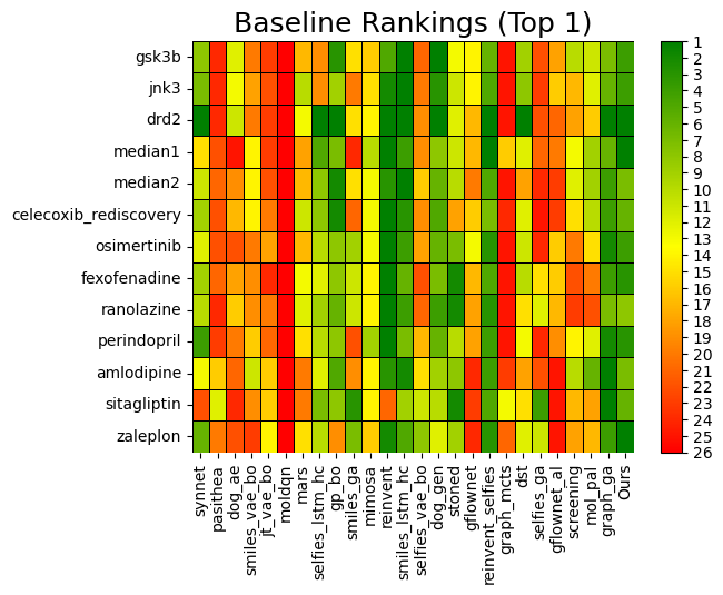
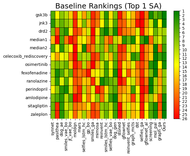
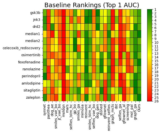
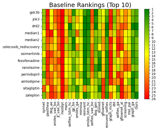
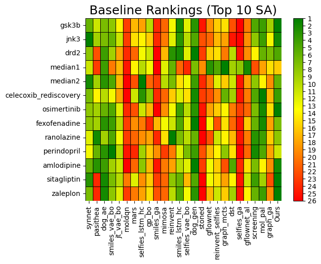
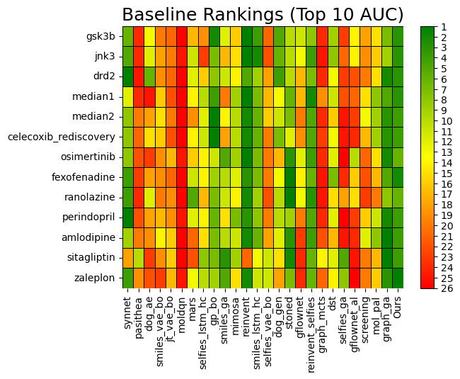
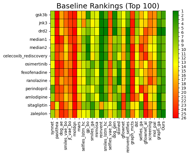
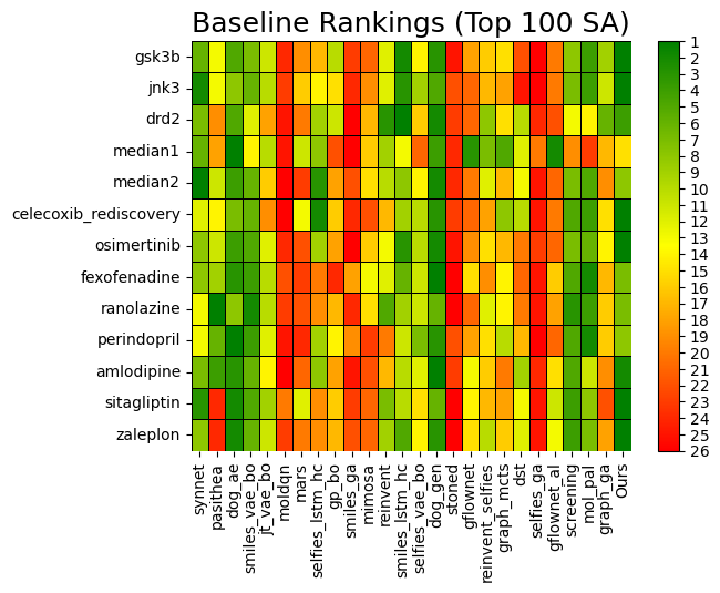
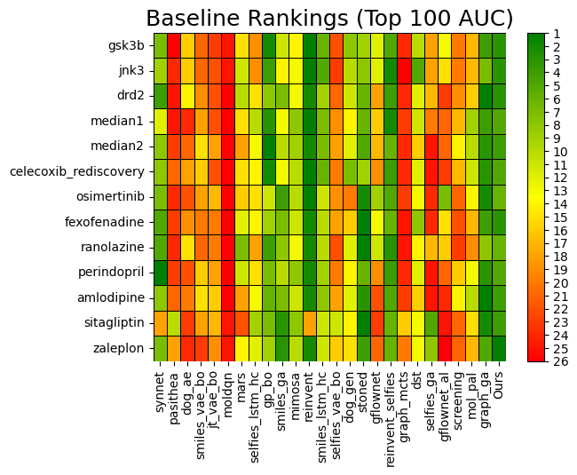
Figure 14: Ranking of our method against baselines on Top $k$ Average Scores (top), SA Scores (middle) and AUC (bottom), for $k=1,10,100$ (left, middle, right).

Appendix H Docking Case Study with AutoDock Vina

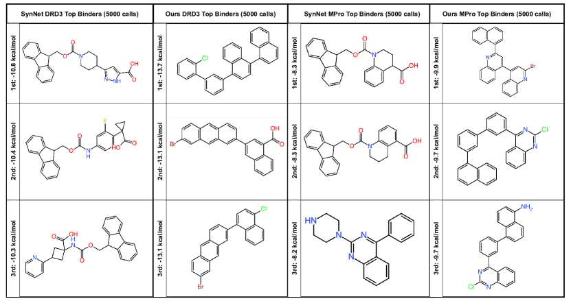
(a) Top 3 molecules with lowest binding energy against DRD3 and MPro from Ours vs SynNet

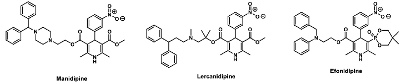
(b) Top sample binders against MPro from literature, based on consensus docking scores [23]

In this section, we structurally analyze the top molecules discovered by our method, visualized in 15(a).

For our optimized binders against DRD3, the chlorine substituent and polycyclic aromatic structure suggest good potential for binding through $\pi-\pi$ interactions and halogen bonding. The bromine and carboxyl groups can enhance binding affinity through halogen bonding and hydrogen bonding, respectively. The polycyclic structure further supports $\pi-\pi$ stacking interactions. In general, they have a comparable binding capability than the baseline molecules, but with simpler structures, the ease of synthesis for the predicted molecules are higher than the baseline molecules.

For our optimized binders against Mpro, the three predicted molecules contain multiple aromatic rings in conjugation with halide groups. The conformation structures of the multiple aligned aromatic rings play a significant role in docking and achieve ideal molecular pose and binding affinity to Mpro, compared with the baseline molecules shown in 15(b). The predicted structures also indicate stronger $\pi-\pi$ interaction and halogen bonding compared with the baselines. In terms of ease of synthesis, Bromination reactions are typically straightforward, but multiple fused aromatic rings can take several steps to achieve. In general, the second and third can be easier to synthesize than Brc1cc(-c2cc(-c3cccc4ccccc34)nc3ccccc23)c2ccccc2n1 due to less aromatic rings performed. However, the literature molecules appeared to be even harder to synthesize due to their high complexicity structures. So the predicted molecules obtained a general higher ease of synthesis than the baseline molecules. Compared with the other baseline molecules, e.g. Manidipine, Lercanidipine, Efonidipine (Dihydropyridines), known for their calcium channel blocking activity, but not specifically protease inhibitors, Azelastine, Cinnoxicam, Idarubicin vary widely in their primary activities, not specifically designed for protease inhibition. Talampicillin and Lapatinib are also primarily designed for other mechanisms of action. Boceprevir, Nelfinavir, Indinavir, on the other hand, are known protease inhibitors with structures optimized for binding to protease active sites, so can serve as strong benchmarks. Overall, the binding effectiveness of the predicted molecules are quite comparable to the baseline molecules.

References

- Alur et al. [2013] R. Alur, R. Bodik, G. Juniwal, M. M. K. Martin, M. Raghothaman, S. A. Seshia, R. Singh, A. Solar-Lezama, E. Torlak, and A. Udupa. Syntax-guided synthesis. In 2013 Formal Methods in Computer-Aided Design, pages 1–8, 2013. doi: 10.1109/FMCAD.2013.6679385.
- Bradshaw et al. [2019] J. Bradshaw, B. Paige, M. J. Kusner, M. Segler, and J. M. Hernández-Lobato. A model to search for synthesizable molecules. Advances in Neural Information Processing Systems, 32, 2019.
- Bradshaw et al. [2020] J. Bradshaw, B. Paige, M. J. Kusner, M. Segler, and J. M. Hernández-Lobato. Barking up the right tree: an approach to search over molecule synthesis dags. Advances in neural information processing systems, 33:6852–6866, 2020.
- Brown et al. [2004] N. Brown, B. McKay, F. Gilardoni, and J. Gasteiger. A graph-based genetic algorithm and its application to the multiobjective evolution of median molecules. Journal of chemical information and computer sciences, 44(3):1079–1087, 2004.
- Bunel et al. [2018] R. Bunel, M. Hausknecht, J. Devlin, R. Singh, and P. Kohli. Leveraging grammar and reinforcement learning for neural program synthesis. arXiv preprint arXiv:1805.04276, 2018.
- Button et al. [2019] A. Button, D. Merk, J. A. Hiss, and G. Schneider. Automated de novo molecular design by hybrid machine intelligence and rule-driven chemical synthesis. Nature machine intelligence, 1(7):307–315, 2019.
- Chen et al. [2020] B. Chen, C. Li, H. Dai, and L. Song. Retro*: learning retrosynthetic planning with neural guided a* search. In Proceedings of the 37th International Conference on Machine Learning, ICML’20. JMLR.org, 2020.
- Chen et al. [2018] X. Chen, C. Liu, and D. Song. Execution-guided neural program synthesis. In International Conference on Learning Representations, 2018.
- Coley et al. [2018] C. W. Coley, W. H. Green, and K. F. Jensen. Machine learning in computer-aided synthesis planning. Accounts of Chemical Research, 51(5):1281–1289, 2018. doi: 10.1021/acs.accounts.8b00087. URL https://doi.org/10.1021/acs.accounts.8b00087. PMID: 29715002.
- Coley et al. [2019] C. W. Coley, D. A. Thomas, J. A. M. Lummiss, J. N. Jaworski, C. P. Breen, V. Schultz, T. Hart, J. S. Fishman, L. Rogers, H. Gao, R. W. Hicklin, P. P. Plehiers, J. Byington, J. S. Piotti, W. H. Green, A. J. Hart, T. F. Jamison, and K. F. Jensen. A robotic platform for flow synthesis of organic compounds informed by ai planning. Science, 365(6453):eaax1566, 2019. doi: 10.1126/science.aax1566. URL https://www.science.org/doi/abs/10.1126/science.aax1566.
- Coley et al. [2020a] C. W. Coley, N. S. Eyke, and K. F. Jensen. Autonomous discovery in the chemical sciences part i: Progress. Angewandte Chemie International Edition, 59(51):22858–22893, 2020a.
- Coley et al. [2020b] C. W. Coley, N. S. Eyke, and K. F. Jensen. Autonomous discovery in the chemical sciences part ii: outlook. Angewandte Chemie International Edition, 59(52):23414–23436, 2020b.
- Corey and Cheng [1989] E. J. Corey and X.-M. Cheng. The logic of chemical synthesis. 1989. URL https://api.semanticscholar.org/CorpusID:94440114.
- Corey et al. [1985] E. J. Corey, A. K. Long, and S. D. Rubenstein. Computer-assisted analysis in organic synthesis. Science, 228(4698):408–418, 1985.
- De Cao and Kipf [2018] N. De Cao and T. Kipf. Molgan: An implicit generative model for small molecular graphs. arXiv preprint arXiv:1805.11973, 2018.
- Dolfus et al. [2022] U. Dolfus, H. Briem, and M. Rarey. Synthesis-aware generation of structural analogues. Journal of Chemical Information and Modeling, 62(15):3565–3576, 2022.
- Ellis et al. [2019] K. Ellis, M. Nye, Y. Pu, F. Sosa, J. Tenenbaum, and A. Solar-Lezama. Write, execute, assess: Program synthesis with a repl. Advances in Neural Information Processing Systems, 32, 2019.
- Ertl and Schuffenhauer [2009] P. Ertl and A. Schuffenhauer. Estimation of synthetic accessibility score of drug-like molecules based on molecular complexity and fragment contributions. Journal of cheminformatics, 1:1–11, 2009.
- Flynn [2014] A. B. Flynn. How do students work through organic synthesis learning activities? Chemistry Education Research and Practice, 15(4):747–762, 2014.
- Gao and Coley [2020] W. Gao and C. W. Coley. The synthesizability of molecules proposed by generative models. Journal of chemical information and modeling, 60(12):5714–5723, 2020.
- Gao et al. [2021] W. Gao, R. Mercado, and C. W. Coley. Amortized tree generation for bottom-up synthesis planning and synthesizable molecular design. arXiv preprint arXiv:2110.06389, 2021.
- Gao et al. [2022] W. Gao, T. Fu, J. Sun, and C. Coley. Sample efficiency matters: a benchmark for practical molecular optimization. Advances in neural information processing systems, 35:21342–21357, 2022.
- Ghahremanpour et al. [2020] M. M. Ghahremanpour, J. Tirado-Rives, M. Deshmukh, J. A. Ippolito, C.-H. Zhang, I. Cabeza de Vaca, M.-E. Liosi, K. S. Anderson, and W. L. Jorgensen. Identification of 14 known drugs as inhibitors of the main protease of sars-cov-2. ACS medicinal chemistry letters, 11(12):2526–2533, 2020.
- Gilks et al. [1995] W. R. Gilks, N. G. Best, and K. K. Tan. Adaptive rejection metropolis sampling within gibbs sampling. Journal of the Royal Statistical Society Series C: Applied Statistics, 44(4):455–472, 1995.
- Guo et al. [2022] M. Guo, V. Thost, B. Li, P. Das, J. Chen, and W. Matusik. Data-efficient graph grammar learning for molecular generation. arXiv preprint arXiv:2203.08031, 2022.
- Hachmann et al. [2011] J. Hachmann, R. Olivares-Amaya, S. Atahan-Evrenk, C. Amador-Bedolla, R. S. Sánchez-Carrera, A. Gold-Parker, L. Vogt, A. M. Brockway, and A. Aspuru-Guzik. The harvard clean energy project: large-scale computational screening and design of organic photovoltaics on the world community grid. The Journal of Physical Chemistry Letters, 2(17):2241–2251, 2011.
- Hartenfeller et al. [2011] M. Hartenfeller, M. Eberle, P. Meier, C. Nieto-Oberhuber, K.-H. Altmann, G. Schneider, E. Jacoby, and S. Renner. A collection of robust organic synthesis reactions for in silico molecule design. Journal of chemical information and modeling, 51(12):3093–3098, 2011.
- Hastings [1970] W. K. Hastings. Monte carlo sampling methods using markov chains and their applications. 1970.
- Huang et al. [2022] K. Huang, T. Fu, W. Gao, Y. Zhao, Y. Roohani, J. Leskovec, C. W. Coley, C. Xiao, J. Sun, and M. Zitnik. Artificial intelligence foundation for therapeutic science. Nature chemical biology, 18(10):1033–1036, 2022.
- Jakubik et al. [2021] J. Jakubik, A. Binding, and S. Feuerriegel. Directed particle swarm optimization with gaussian-process-based function forecasting. European Journal of Operational Research, 295(1):157–169, 2021.
- Janet et al. [2020] J. P. Janet, S. Ramesh, C. Duan, and H. J. Kulik. Accurate multiobjective design in a space of millions of transition metal complexes with neural-network-driven efficient global optimization. ACS central science, 6(4):513–524, 2020.
- Jin et al. [2018] W. Jin, R. Barzilay, and T. Jaakkola. Junction tree variational autoencoder for molecular graph generation. In International conference on machine learning, pages 2323–2332. PMLR, 2018.
- Jin et al. [2020] W. Jin, R. Barzilay, and T. Jaakkola. Hierarchical generation of molecular graphs using structural motifs. In International conference on machine learning, pages 4839–4848. PMLR, 2020.
- Kirkpatrick et al. [1983] S. Kirkpatrick, C. D. Gelatt Jr, and M. P. Vecchi. Optimization by simulated annealing. science, 220(4598):671–680, 1983.
- Koch et al. [2015] P. Koch, M. Gehringer, and S. A. Laufer. Inhibitors of c-jun n-terminal kinases: an update. Journal of medicinal chemistry, 58(1):72–95, 2015.
- Koscher et al. [2023] B. A. Koscher, R. B. Canty, M. A. McDonald, K. P. Greenman, C. J. McGill, C. L. Bilodeau, W. Jin, H. Wu, F. H. Vermeire, B. Jin, et al. Autonomous, multiproperty-driven molecular discovery: From predictions to measurements and back. Science, 382(6677):eadi1407, 2023.
- Levin et al. [2023] I. Levin, M. E. Fortunato, K. L. Tan, and C. W. Coley. Computer-aided evaluation and exploration of chemical spaces constrained by reaction pathways. AIChE journal, 69(12):e18234, 2023.
- Li et al. [2018] Y. Li, O. Vinyals, C. Dyer, R. Pascanu, and P. Battaglia. Learning deep generative models of graphs. arXiv preprint arXiv:1803.03324, 2018.
- Liu et al. [2018] Q. Liu, M. Allamanis, M. Brockschmidt, and A. Gaunt. Constrained graph variational autoencoders for molecule design. Advances in neural information processing systems, 31, 2018.
- Lyu et al. [2019] J. Lyu, S. Wang, T. E. Balius, I. Singh, A. Levit, Y. S. Moroz, M. J. O’Meara, T. Che, E. Algaa, K. Tolmachova, et al. Ultra-large library docking for discovering new chemotypes. Nature, 566(7743):224–229, 2019.
- Ma et al. [2018] T. Ma, J. Chen, and C. Xiao. Constrained generation of semantically valid graphs via regularizing variational autoencoders. Advances in Neural Information Processing Systems, 31, 2018.
- Madras [2013] B. K. Madras. History of the discovery of the antipsychotic dopamine d2 receptor: a basis for the dopamine hypothesis of schizophrenia. Journal of the History of the Neurosciences, 22(1):62–78, 2013.
- McCorkindale [2023] W. McCorkindale. Accelerating the Design-Make-Test cycle of Drug Discovery with Machine Learning. PhD thesis, 2023.
- Merrell [2023] P. Merrell. Example-based procedural modeling using graph grammars. ACM Transactions on Graphics (TOG), 42(4):1–16, 2023.
- Merrell and Manocha [2010] P. Merrell and D. Manocha. Model synthesis: A general procedural modeling algorithm. IEEE transactions on visualization and computer graphics, 17(6):715–728, 2010.
- Merrell et al. [2011] P. Merrell, E. Schkufza, Z. Li, M. Agrawala, and V. Koltun. Interactive furniture layout using interior design guidelines. In ACM SIGGRAPH 2011 Papers, SIGGRAPH ’11, New York, NY, USA, 2011. Association for Computing Machinery. ISBN 9781450309431. doi: 10.1145/1964921.1964982. URL https://doi.org/10.1145/1964921.1964982.
- Metropolis et al. [1953] N. Metropolis, A. W. Rosenbluth, M. N. Rosenbluth, A. H. Teller, and E. Teller. Equation of state calculations by fast computing machines. The journal of chemical physics, 21(6):1087–1092, 1953.
- Müller et al. [2006] P. Müller, P. Wonka, S. Haegler, A. Ulmer, and L. Van Gool. Procedural modeling of buildings. In ACM SIGGRAPH 2006 Papers, pages 614–623. 2006.
- Polikarpova et al. [2016] N. Polikarpova, I. Kuraj, and A. Solar-Lezama. Program synthesis from polymorphic refinement types. ACM SIGPLAN Notices, 51(6):522–538, 2016.
- Qiang et al. [2023] B. Qiang, Y. Zhou, Y. Ding, N. Liu, S. Song, L. Zhang, B. Huang, and Z. Liu. Bridging the gap between chemical reaction pretraining and conditional molecule generation with a unified model. Nature Machine Intelligence, 5(12):1476–1485, 2023.
- Samanta et al. [2020] B. Samanta, A. De, G. Jana, V. Gómez, P. Chattaraj, N. Ganguly, and M. Gomez-Rodriguez. Nevae: A deep generative model for molecular graphs. Journal of machine learning research, 21(114):1–33, 2020.
- Sanchez-Lengeling and Aspuru-Guzik [2018] B. Sanchez-Lengeling and A. Aspuru-Guzik. Inverse molecular design using machine learning: Generative models for matter engineering. Science, 361(6400):360–365, 2018. doi: 10.1126/science.aat2663. URL https://www.science.org/doi/abs/10.1126/science.aat2663.
- Schkufza et al. [2013] E. Schkufza, R. Sharma, and A. Aiken. Stochastic superoptimization. SIGPLAN Not., 48(4):305–316, mar 2013. ISSN 0362-1340. doi: 10.1145/2499368.2451150. URL https://doi.org/10.1145/2499368.2451150.
- Shi et al. [2020] Y. Shi, Z. Huang, S. Feng, H. Zhong, W. Wang, and Y. Sun. Masked label prediction: Unified message passing model for semi-supervised classification. arXiv preprint arXiv:2009.03509, 2020.
- Simonovsky and Komodakis [2018] M. Simonovsky and N. Komodakis. Graphvae: Towards generation of small graphs using variational autoencoders. In Artificial Neural Networks and Machine Learning–ICANN 2018: 27th International Conference on Artificial Neural Networks, Rhodes, Greece, October 4-7, 2018, Proceedings, Part I 27, pages 412–422. Springer, 2018.
- Smith [1997] W. D. Smith. Computational complexity of synthetic chemistry–basic facts. Technical report, Citeseer, 1997.
- Solar-Lezama et al. [2005] A. Solar-Lezama, R. Rabbah, R. Bodík, and K. Ebcioğlu. Programming by sketching for bit-streaming programs. In Proceedings of the 2005 ACM SIGPLAN conference on Programming language design and implementation, pages 281–294, 2005.
- Sun et al. [2017] J. Sun, N. Jeliazkova, V. Chupakhin, J.-F. Golib-Dzib, O. Engkvist, L. Carlsson, J. Wegner, H. Ceulemans, I. Georgiev, V. Jeliazkov, et al. Excape-db: an integrated large scale dataset facilitating big data analysis in chemogenomics. Journal of cheminformatics, 9:1–9, 2017.
- Sun et al. [2024] M. Sun, M. Guo, W. Yuan, V. Thost, C. E. Owens, A. F. Grosz, S. Selvan, K. Zhou, H. Mohiuddin, B. J. Pedretti, et al. Representing molecules as random walks over interpretable grammars. arXiv preprint arXiv:2403.08147, 2024.
- Swanson et al. [2024] K. Swanson, G. Liu, D. B. Catacutan, A. Arnold, J. Zou, and J. M. Stokes. Generative ai for designing and validating easily synthesizable and structurally novel antibiotics. Nature Machine Intelligence, 6(3):338–353, 2024.
- Talton et al. [2011] J. O. Talton, Y. Lou, S. Lesser, J. Duke, R. Mech, and V. Koltun. Metropolis procedural modeling. ACM Trans. Graph., 30(2):11–1, 2011.
- Tian et al. [2018] J. Tian, Y. Tan, J. Zeng, C. Sun, and Y. Jin. Multiobjective infill criterion driven gaussian process-assisted particle swarm optimization of high-dimensional expensive problems. IEEE Transactions on Evolutionary Computation, 23(3):459–472, 2018.
- Torren-Peraire et al. [2024] P. Torren-Peraire, A. K. Hassen, S. Genheden, J. Verhoeven, D.-A. Clevert, M. Preuss, and I. V. Tetko. Models matter: the impact of single-step retrosynthesis on synthesis planning. Digital Discovery, 3(3):558–572, 2024.
- Tu et al. [2022] H. Tu, S. Shorewala, T. Ma, and V. Thost. Retrosynthesis prediction revisited. In NeurIPS 2022 AI for Science: Progress and Promises, 2022.
- Vinkers et al. [2003] H. M. Vinkers, M. R. de Jonge, F. F. Daeyaert, J. Heeres, L. M. Koymans, J. H. van Lenthe, P. J. Lewi, H. Timmerman, K. Van Aken, and P. A. Janssen. Synopsis: synthesize and optimize system in silico. Journal of medicinal chemistry, 46(13):2765–2773, 2003.
- Volkamer et al. [2023] A. Volkamer, S. Riniker, E. Nittinger, J. Lanini, F. Grisoni, E. Evertsson, R. Rodríguez-Pérez, and N. Schneider. Machine learning for small molecule drug discovery in academia and industry. Artificial Intelligence in the Life Sciences, 3:100056, 2023.
- Yao et al. [2021] Z. Yao, B. Sánchez-Lengeling, N. S. Bobbitt, B. J. Bucior, S. G. H. Kumar, S. P. Collins, T. Burns, T. K. Woo, O. K. Farha, R. Q. Snurr, et al. Inverse design of nanoporous crystalline reticular materials with deep generative models. Nature Machine Intelligence, 3(1):76–86, 2021.
- You et al. [2018] J. You, B. Liu, Z. Ying, V. Pande, and J. Leskovec. Graph convolutional policy network for goal-directed molecular graph generation. Advances in neural information processing systems, 31, 2018.
- Yu et al. [2011] L.-F. Yu, S.-K. Yeung, C.-K. Tang, D. Terzopoulos, T. F. Chan, and S. J. Osher. Make it home: automatic optimization of furniture arrangement. ACM Trans. Graph., 30(4), jul 2011. ISSN 0730-0301. doi: 10.1145/2010324.1964981. URL https://doi.org/10.1145/2010324.1964981.
- Zhang et al. [2021] C.-H. Zhang, E. A. Stone, M. Deshmukh, J. A. Ippolito, M. M. Ghahremanpour, J. Tirado-Rives, K. A. Spasov, S. Zhang, Y. Takeo, S. N. Kudalkar, et al. Potent noncovalent inhibitors of the main protease of sars-cov-2 from molecular sculpting of the drug perampanel guided by free energy perturbation calculations. ACS central science, 7(3):467–475, 2021.
- Zhang et al. [2019] Y. Zhang, H. Li, E. Bao, L. Zhang, and A. Yu. A hybrid global optimization algorithm based on particle swarm optimization and gaussian process. International Journal of Computational Intelligence Systems, 12(2):1270–1281, 2019.
- Zhavoronkov et al. [2019] A. Zhavoronkov, Y. A. Ivanenkov, A. Aliper, M. S. Veselov, V. A. Aladinskiy, A. V. Aladinskaya, V. A. Terentiev, D. A. Polykovskiy, M. D. Kuznetsov, A. Asadulaev, et al. Deep learning enables rapid identification of potent ddr1 kinase inhibitors. Nature biotechnology, 37(9):1038–1040, 2019.
- Zimmerman et al. [2020] J. B. Zimmerman, P. T. Anastas, H. C. Erythropel, and W. Leitner. Designing for a green chemistry future. Science, 367(6476):397–400, 2020.