A Framework for Evaluating PM2.5 Forecasts from the Perspective of Individual Decision Making

Abstract

Wildfire frequency is increasing as the climate changes, and the resulting air pollution poses health risks. Just as people routinely use weather forecasts to plan their activities around precipitation, reliable air quality forecasts could help individuals reduce their exposure to air pollution. In the present work, we evaluate several existing forecasts of fine particular matter (PM2.5) within the continental United States in the context of individual decision-making. Our comparison suggests there is meaningful room for improvement in air pollution forecasting, which might be realized by incorporating more data sources and using machine learning tools. To facilitate future machine learning development and benchmarking, we set up a framework to evaluate and compare air pollution forecasts for individual decision making. We introduce a new loss to capture decisions about when to use mitigation measures. We highlight the importance of visualizations when comparing forecasts. Finally, we provide code to download and compare archived forecast predictions.

1 Introduction

Exposure to elevated levels of PM2.5 can result in severe health consequences, including respiratory and cardiovascular diseases [15, 18, 28]. Even short-term air exposure can be detrimental [15]. In the face of increased wildfire events due to climate change [33, 30, 32], forecasts that identify when and where to expect acute air pollution events, often due to smoke [26, 6], can allow both governments and individuals to mitigate exposure risk. Many people rely on weather forecasts to plan when to go outside, whether to walk or drive to work, or whether to carry an umbrella. Analogously, a reliable air quality forecast could allow an individual with a respiratory condition to decide when to complete household chores, whether to work from home, or whether to wear a respirator.

Currently, forecasts of air quality are produced by simulations of atmospheric conditions. Given the saliency of wildfire smoke to extreme pollution events in the United States, we here select forecasts that include near-real-time updates to the smoke PM2.5 emitted from wildland fires. These forecasts have been validated in scientific studies for their ability to capture broad trends and specific major pollution events arising from short-range smoke transport [41, 8, 42, 25, 11]. [2], however, emphasize the importance of aligning evaluation metrics with the intended use of a forecast. Based on Canadian air quality guidance and a survey of officials in western Canada, they assess whether a particular forecast, the Canada FireWork model [9], correctly identified days with PM2.5 levels exceeding 25 $\mu$g/m³. This assessment captures how reliably individuals can decide whether or not to take mitigation measures at the granularity of a day. However, we observe (1) that individuals would often like to make decisions based on air quality within a single day. (2) There are multiple major forecast models, and it is presently unclear which offers the most accurate forecasts (in any sense) within the continental US. And (3) while [2] provide links to data sources, actually retrieving and standardizing the data from these and other sources is currently labor intensive and time consuming. Our work addresses these issues.

Our principal contribution is the development of a framework to assess PM2.5 forecasts for individual decision-making and to facilitate machine-learning benchmarks. Our framework includes a suite of evaluation tools to capture different aspects of individual decision making. As part of this suite, we introduce a new metric, mean excess exposure, to capture the impacts of using hourly forecasts for decision making. Since the complexities of individual decisions cannot be fully captured by a single metric, we advocate for the visualization of forecasts during extreme events. We demonstrate the usefulness of our framework by evaluating four existing PM2.5 forecast models during high-smoke events. We find that no single forecast consistently outperforms the others across evaluation metrics and that there remains substantial room for improvement. Finally, we provide code for downloading data archives for all forecast products considered, as well as a simple persistence baseline. We conclude with a discussion of the promise for machine learning to improve existing forecasts.

2 Ground Truth, Existing Forecasts, and Persistence Baseline

We first establish the data we use for ground truth, the forecasts we compare, and the baseline we use.

Ground Truth. To assess air quality forecasts, we compare to observed air quality data. The State and Local Monitoring Systems (SLAMS) consist of federal regulatory monitors and federal equivalence monitors. SLAMS measurements of surface-level PM2.5 are considered high quality, but they are geographically sparse. The EPA requires monitors to be placed in areas with high populations or areas believed to have high levels of air pollution, with the actual placement of monitors left up to state and local agencies. So there are potential geographical biases, such as undercoverage of rural areas. Low-cost sensor networks, such as PurpleAir, offer better spatial coverage. However, the sensors are believed to make substantially larger measurement errors than regulatory monitors, including overestimation of PM2.5 concentrations during extreme smoke events [21]. We treat SLAMS as ground truth. We focus our analysis on large metropolitan areas, both because these regions cover so much of the US population and because we have access to validation data there.

Existing Forecasts. Due to the public health implications of air pollution, multiple government agencies have produced PM2.5 forecasts. We evaluate four forecasts: (1) the High Resolution Rapid-Refresh Smoke (HRRR-Smoke) model from the National Oceanic and Atmospheric Administration (NOAA) [16]; (2) the Copernicus Atmosphere Monitoring Service Forecast (CAMS) from the European Centre for Medium-Range Weather Forecasts (ECMWF) [34]; (3) the Global Earth Observing System Composition Forecasting (GEOS-CF) model from NASA’s Global Modeling and Assimilation Office (GMAO) [23]; and (4) the National Air Quality Forecast Capability (NAQFC) from NOAA and the National Weather Service (NWS) [13, 39]. Our analysis is not intended to be exhaustive but rather to provide a set of sensible baselines for comparison to machine learning approaches. We provide more detail, and additional forecast references, in appendix A.

Persistence Baseline. [2] advocate for a baseline forecast that predicts air quality will remain constant for the next 24 hours. We construct this baseline from monitor data and historical readings produced by SLAMS and publicly available through the EPA [1].

3 Metrics and Visualizations

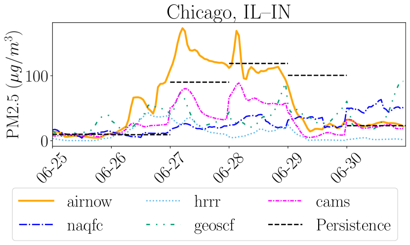
	TP	FP	FN	TN	MEE
HRRR	2	0	12	170	10.2
GEOS-CF	14	129	0	41	8.2
CAMS	9	4	5	166	3.3
NAQFC	9	15	5	155	8.9
Persistence	6	1	8	169	17.3

Figure 1: Left: Forecasts (dotted light blue, dashdot fuchsia, densely dashdotted blue, dashdotdotted green), measured air quality (solid orange), and the persistence baseline (dashed black) for the Chicago metro area during an extreme event in 2023. High levels of PM2.5 were caused by the transport of wildfire smoke. Right: Confusion matrix for predicting extreme events (days with measured PM2.5 concentration above $35\mu$g/m³) in Chicago for each forecast and the persistence baseline. The columns TP, FP, FN, and TN represent True Positive, False Positive, False Negative, and True Negative, respectively. Cells are shaded red if the forecast performs worse than the baseline (lower TP, TN; higher FP, FN, or MEE), green if the forecast performs better than the baseline.

We next describe the metrics we use to evaluate forecast quality and compare forecasts. Since no single statistic can fully capture the nuances of individual decision-making, we also advocate plotting forecasts alongside actual air quality over time for specific cities during extreme events. Further details of the metrics we describe can be found in appendix B. Although we report root mean square error (RMSE) in appendix D, we do not recommend it for individual decision-making as it lacks clear interpretation in this context.

When should we go out during the day? Mean Excess Exposure. We introduce a metric to capture how useful a forecast is for the following individual decision-making process. We imagine someone who needs to spend an hour outside, is flexible about when to go outside, wants to minimize PM2.5 exposure, and will use the morning forecast to make their decision. We define the individual excess exposure for day $d$ and location $s$ as (1) the PM2.5 exposure that results from someone choosing the best hour from the potentially-erroneous forecast minus (2) the PM2.5 exposure of a person who chooses the best hour given the ground-truth PM2.5 concentrations for the day. For day $d$ and location $s$, the minimum potential exposure is $\min_{h\in\{1,\dots,24\}}\mathrm{PM2.5}_{d,s}(h)$, where $\mathrm{PM2.5}_{d,s}(h)$ is the concentration at hour $h$. For a forecast that predicts $\widehat{\mathrm{PM2.5}}_{d,s}(h)$, define

$$\smash{\mathrm{EE}(d,s)=\mathrm{PM2.5}_{d,s}(\arg\min_{h\in\{1,\dots,24\}}\widehat{\mathrm{PM2.5}}_{d,s}(h))-\min_{h\in\{1,\dots,24\}}\mathrm{PM2.5}_{d,s}(h).}$$ (1)

For a collection of days $\cal{T}$ and a particular forecast we compute the mean excess exposure (MEE) as $\frac{1}{|\cal{T}|}\sum_{d\in\cal{T}}\mathrm{EE}(d,s).$ Shifting or scaling the predictions of a forecast uniformly over time has no effect on the forecast’s MEE. Since all hours offer equivalent exposure under the persistence baseline, we treat the MEE of the persistence baseline as the MEE of a uniformly random hour during the day.

Should we go out today? Confusion matrices for extreme events. After consulting the morning forecast, an individual in a sensitive group might decide to work from home on a day when exposure exceeds a certain threshold, such as the Environmental Protection Agency’s 24-hour limit of 35$\mu$g/m³. We therefore construct the confusion matrix for whether a forecast accurately predicts exceedance of this threshold. This analysis is similar to that of [2], which was motivated by public health alerts.

Table 1: Aggregated confusion matrix and MEE for all 30 cities in appendix D. Cells are shaded red if the forecast performs worse than the baseline (lower TP, TN; higher FP, FN, or MEE), green if the forecast performs better than the baseline, and not shaded if the forecast is as good as the baseline.

Model	True Positive	False Positive	False Negative	True Negative	MEE
hrrr	27	7	192	4917	12.26
geoscf	169	1928	50	2996	10.83
cams	79	41	140	4883	10.48
naqfc	64	129	155	4795	10.53
persistence	69	7	150	4917	19.27

4 An Example of Our Framework Applied to Current Forecasts

Given space constraints in the main text, we focus on the Chicago urban area during the period from May 1^st to October 31^st, 2023, specifically on the 14 days when PM2.5 levels were elevated (with daily maximum concentrations exceeding 35 $\mu$g/m³). We provide a comprehensive analysis of two additional metropolitan areas, San Francisco and Philadelphia, in appendix C. We provide summary statistics across 30 cities among the largest metropolitan areas in continental US in appendix D.

When should we go out today? Current forecasts outperform the baseline. All forecasts show MEE improvements over the persistence baseline; see the right table in fig. 1 for Chicago and table 1 for the 30 cities. That is, our analysis suggests that the forecasts can be useful for identifying the hour of lowest exposure during the day. However, individuals are still exposed to substantially more PM2.5 than they would be if they knew the true air quality throughout the day in advance.

Should we go out today? Current forecasts do not outperform the baseline. All forecasts struggle with accurately classifying extreme events. For Chicago (table in fig. 1), HRRR correctly identifies only 2 of the 14 high PM2.5 days, while GEOS-CF identifies all 14 but generates 129 false positives. CAMS and NAQFC identify 9 out of 14 high PM2.5 days but also produce more false positives compared to the baseline, which has only 1. Across the 30 cities (table 1), none of the forecasts outperform the baseline, and most perform worse. [2] similarly found that when predictions were taken at face value, the Canada FireWork forecast did not outperform the persistence baseline during the 2016–2018 fire seasons in western Canada.

Visual evaluations reveal forecast limitations not captured by metrics. Especially in the MEE metric (table in fig. 1), CAMS stands out among the four models. However, we see from the left plot (fig. 1) that CAMS only vaguely identifies the magnitude or timing of a PM2.5 peak. The situation is even worse during the San Francisco week appearing in fig. 2; while all methods show some MEE benefit, the left plot reveals that they all fail to capture almost all meaningful structure of the major pollution event. While we argue that visualization is an essential supplement to metrics, we also note that visualizing every extreme event across all cities in the continental US would be impractical. That is, metrics and visualizations form complementary parts of a comprehensive evaluation.

Current forecasts can help with individual decision making, but there remains a substantial performance gap relative to an oracle. The improvements in MEE relative to the persistence baseline suggest that the forecasts we consider provide some useful information for individuals making decisions. However, these forecasts can still lead to dramatically suboptimal decision-making in many situations. Figure 2 shows a case where forecasts fail to predict almost any aspect of the timing or magnitude of an extreme PM2.5 event caused by fire smoke. While not every failure is as dramatic (cf. fig. 1), our analysis across 30 cities shows that forecasts systematically miss many key decision-making elements of major fire-smoke pollution events.

There is reason for optimism that the observed performance gap might be at least partly filled by machine learning. Current forecasts are based on simulating atmospheric conditions for formation and transport of PM2.5. Near-real-time data is used in setting the initial conditions of the simulation. Additionally, aspects of the physics that cannot be simulated due to computational constraints are parameterized, and these parameters are calibrated to historical data. However, this calibration is not necessarily targeted to the task of improving the accuracy of air quality forecasts, as the atmospheric simulations produce many other outputs that are also of interest to the agency releasing the forecasts. Furthermore, many of the forecasts available are global models, and their calibration cannot be targeted at specific locations. There are numerous data sources – for example historical satellite observations [44, 31], meteorological records [35], and ground-based PM2.5 sensors [1] – that should be informative about the relationship between current conditions and future PM2.5 pollution levels. By combining a data-driven approach with physical understanding, we can develop more robust forecasts that better serve individuals seeking to minimize their exposure to air pollution.

Appendix A Detailed Description of Forecasts

In this section, we describe the forecasts that we evaluate. All of the forecasts provide archived predictions, which are used in the analysis. For each forecast, we (1) provide key citations and a brief overview of the approach; (2) state spatial resolution and extent; and (3) state the frequency at which predictions are made and how far forward the forecast goes.

High Resolution Rapid-Refresh Smoke (HRRR-Smoke)

High resolution rapid refresh (HRRR) is a numerical weather prediction model released and maintained by the National Oceanic and Atmospheric Administration (NOAA) [16]. HRRR operates on 3km resolution over the extent of the contiguous United States and Alaska. 18 hour forecasts for the continental United States are run hourly, with forecasts as far forward as 48 hours made every 6 hours. Smoke sources are detected using remote sensing of fire radiative power, and transport of smoke is integrated into the numerical weather prediction model and uses a simplified version of WRF-chem [19]. As HRRR-Smoke accounts for only smoke sources that can be detected with remote sensing (wildfires and prescribed burns), we expect it to systematically underestimate PM2.5 levels, particularly in locations where there are significant anthropogenic sources of fine particulate matter. However, in the United States extreme levels of fine particulate matter (for example, exceeding the EPA 24 hour exposure guidance of 35$\mu$g/m³) are often driven by fire smoke [29]. HRRR-Smoke therefore is a plausible tool for forecasting intensity and timing of extremely elevated fine particulate matter events in the continental United States.

Copernicus Atmosphere Monitoring Service Forecast (CAMS)

The Copernicus Atmosphere Monitoring Service (CAMS) is an air quality and atmospheric composition forecast system developed by the European Centre for Medium-Range Weather Forecasts (ECMWF) as part of the ECMWF Integrated Forecast System [34]. CAMS provides global and regional forecasts of atmospheric composition, including concentrations of key pollutants such as particulate matter (PM2.5), ozone, and nitrogen dioxide. The model operates at an effective horizontal resolution of 0.4°, approximately 40 km, making it suitable for broad-scale analysis over large regions. CAMS integrates data from multiple sources, including satellite observations and ground-based measurements, to produce forecasts of air quality. However, due to its relatively coarse resolution, CAMS may not capture localized pollution events as precisely as higher-resolution models. Given that CAMS incorporates a comprehensive range of emission sources, including anthropogenic activities, it could plausibly produce less biased forecasts of PM2.5 levels than models focusing solely on fire sources like HRRR-Smoke.

GEOS Composition Forecasting (GEOS-CF)

The Global Earth Observing System Composition Forecasting (GEOS-CF) model is developed and maintained by NASA’s Global Modeling and Assimilation Office (GMAO) [23]. GEOS-CF provides global air quality forecasts, leveraging the GEOS Atmospheric General Circulation Model and a sophisticated data assimilation system (hybrid-4DEnVar ADAS) [17]. The model operates at a spatial resolution of 0.25° (approximately 25 km) and includes 72 vertical layers. GEOS-CF runs 5-day forecasts once per day, offering both high temporal resolution products with outputs every 15 minutes or hourly, which can be either time-averaged or instantaneous. The model integrates a wide range of emission sources, including near-real-time biomass burning emissions from the Quick Fire Emission Database (QFED v2.5) [12] and anthropogenic emissions from the HTAP v2.2 and RETRO inventories [22, 38], which are broken down into hourly values using sector-specific day-of-week and diurnal scale factors [14]. Aerosols, an integral component of the model physics, are simulated with the GOCART model [10], incorporating both anthropogenic and biogenic emissions.

National Air Quality Forecast Capability (NAQFC)

The National Air Quality Forecast Capability (NAQFC) integrates the North American Mesoscale (NAM) Forecast System with the Community Multiscale Air Quality (CMAQ) modeling system, developed and maintained by NOAA and the National Weather Service (NWS) [13, 39]. NAQFC provides air quality forecasts up to 48 hours out, issued twice daily at 6 and 12 UTC, covering the contiguous United States, Alaska, and Hawaii at a spatial resolution of approximately 12 km. The model operates using NOAA’s operational FV3-GFSv16 meteorology and includes 35 vertical layers, enabling detailed simulations of atmospheric processes [7]. NAQFC employs static chemical gaseous boundary conditions from global GEOS-Chem simulations, while aerosol boundary conditions are dynamically updated from NOAA’s operational GEFS-Aerosols model [43]. Biomass-burning emissions are incorporated into the model via the GBBEPx system, with wildfire smoke plumes computed using the Briggs plume rise algorithm [5]. Additionally, NAQFC accounts for anthropogenic and biogenic emissions, providing a comprehensive representation of various emission sources affecting air quality. Fire emissions are integrated into PM2.5 concentration forecasts using the BlueSky framework [24]. NAQFC’s capability to forecast PM2.5 was released in 2015/2016, much later than its ozone forecasts, and has undergone continuous improvements to better capture the effects of fires and extreme pollution events. Despite its robust framework, the model faces challenges in accurately predicting air quality during extreme events, as noted in NOAA’s documentation [36]. To address some of these challenges, bias correction approaches have been explored to improve NAQFC’s predictions of PM2.5 levels during such events [20].

Forecasts we do not consider

While we consider many of the physics-driven forecasts produced by government agencies, we do not compute metrics for the Navy Aerosol Analysis and Prediction System (NAAPS) forecast. We also do not consider ensemble approaches (beyond any ensembling used implicitly in the forecasts), such as the multi-agency ensemble produced in [27]. We do not include the recent Aurora model, which takes a foundation model approach to the forecasting problem [3], as at the time of submission the air quality forecasting components of the model are not publicly available. Similarly, we do not include BreezoMeter [4] which uses a combination of the CAMS and machine learning to make forecasts because the data is not available without payment. We expect that additional forecasts will be introduced as machine learning and data-driven approaches are applied to this problem. And the introduction of a common suite of metrics and benchmark datasets has aided the rapid growth of data-driven weather forecasts [37]. We do not intend our analysis to be exhaustive, but to provide an illustration of the framework we develop and a handful of sensible baselines for comparison to machine learning approaches, that can be added to as improvements in forecasting are made.

Using low-cost sensor data for validation

Incorporating low-cost sensor data, e.g. PurpleAir, into a validation procedure could improve understanding of forecast quality throughout the continental United States, but this approach requires additional consideration of how to account for measurement biases in the validation process.

Appendix B Additional Details of Computation of Metrics

B.1 Timing of Forecasts Used

For all forecasts, we use the version of the forecasts run at 12UTC. We compare forecasts over a 24-hour window beginning at 13UTC and running until 12UTC the following day. The persistence model is calculated using the monitor reading at 10UTC the previous day. The GEOS-CF forecast computes both time-averaged (over an hour) and instantaneous forecast products. We use the time averaged version, and associate the forecast to the hour after before is made. That is, the forecast between 12UTC and 13UTC is associated to 12UTC.

B.2 Spatial Averaging and Interpolation

Forecast predictions are not generally available at the exact locations of PM2.5 monitors. To compute the “ground truth” PM2.5 for a metropolitan area, we use latitude and longitude data provided by the US Census Gazetteer list of Urban Areas [40]. We perform a nearest-neighbors search using the Haversine distance to find the nearest active monitors within a 10 km radius of each metropolitan area, with a maximum of 10 neighbors included. If the metropolitan areas had no PM2.5 monitors within a 10km radius of the latitude and longitude provided in the gazetteer, we expanded the radius of monitors included to 50km. The PM2.5 concentration for the metropolitan area is then calculated as the average of the PM2.5 concentrations measured by all included monitors. For the predicted PM2.5, we use all prediction within a fixed radius of the latitude and longitude used for the metropolitan area. We use a radius of 50km for HRRR-Smoke, GEOS-CF and NAQFC and a radius of 60km for CAMS due to its coarser spatial resolution.

B.3 Missing Data

We exclude days from the analysis if no PM2.5 monitors are active (for example if they are down for maintenance) near a given metropolitan area for any hour during the day.

B.4 Tie-breaking

If several hours in the day have the same predicted PM2.5 and this predicted PM2.5 is the minimum predicted over the day, we compute the excess exposure using the earliest of these hours.

Appendix C Additional City-Level Analysis

In this appendix, we extend the analysis presented for Chicago to two additional metropolitan areas: San Francisco and Philadelphia during Summer 2023. In both cases, elevated PM2.5 levels were similarly attributed to the transport of wildfire smoke.

C.1 Chicago Metropolitan Area

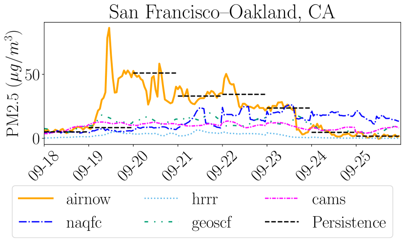
	TP	FP	FN	TN	MEE
HRRR	0	0	8	174	5.1
GEOS-CF	1	10	7	164	5.2
CAMS	0	0	8	174	9.5
NAQFC	0	0	8	174	5.5
Persistence	1	0	7	174	11

Figure 2: Left: Forecasts (dotted light blue, dashdot fuchsia, densely dashdotted blue, dashdotdotted green), measured air quality (solid orange), and the persistence baseline (dashed black) for the San Francisco metropolitan area during an extreme event in 2023. High levels of PM2.5 were caused by the transport of wildfire smoke. Right: Confusion matrix for predicting extreme events (days with measured PM2.5 concentration above $35\mu$g/m³) in San Francisco for each forecast and the persistence baseline. The columns TP, FP, FN, and TN in the confusion matrix represent True Positive, False Positive, False Negative, and True Negative, respectively. Cells are shaded red if the forecast performs worse than the baseline (lower TP, TN; higher FP, FN, or MEE), green if the forecast performs better than the baseline, and not shaded if the forecast is as good as the baseline.

In this section, we analyze San Francisco from May 1 to October 31, 2023, focusing on days when PM2.5 levels were elevated, defined as days with maximum measured concentrations exceeding 35 $\mu$g/m³. There were 8 such days within this period.

First, we observe a pattern similar to what we noted for San Francisco in the main text: when we assess the forecasts using MEE, as shown in the MEE column of the table in fig. 2, all forecasts show improvements over the persistence baseline. This indicates that forecasts may be useful for individuals seeking to identify the safest times to go outside during the day.

Next, even though MEE values surpass the baseline, the forecasts still struggle to accurately classify extreme events. In particular, no forecast correctly identified more than one of eight high PM2.5 days. While GEOS-CF predicted one high day, it also generated 10 false positives; see the four leftmost columns in the table in fig. 2. This supports the conclusion from the main text that current forecasts are not yet reliable enough for individuals making decisions based on whether PM2.5 levels will exceed the EPA’s 24-hour regulatory level.

Finally, the left plot in fig. 2 further underscores the importance of visualizing predictions over time to better evaluate the utility of forecasts for individual decision-making. Although MEE for all four forecasts is better than the persistence baseline, the plot shows that during a week in September 2023, none of the forecasts accurately predicted the magnitude or timing of PM2.5 peaks. This suggests that while MEE is valuable for those individuals seeking the optimal time to go outside, it can be less effective for other kind of individuals, e.g. those primarily concerned with avoiding peak exposure.

C.2 Philadelphia Metropolitan Area

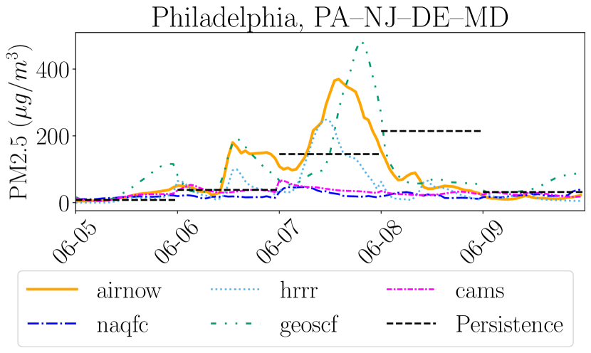
	TP	FP	FN	TN	MEE
HRRR	4	1	9	170	10.3
GEOS-CF	13	120	0	51	15.5
CAMS	5	2	8	169	19.0
NAQFC	6	11	7	160	16.3
Persistence	6	0	7	171	29.7

Figure 3: Left: Forecasts (dotted light blue, dashdot fuchsia, densely dashdotted blue, dashdotdotted green), measured air quality (solid orange), and the persistence baseline (dashed black) for the Philadelphia metropolitan area during an extreme event in 2023. High levels of PM2.5 were caused by the transport of wildfire smoke. Right: Confusion matrix for predicting extreme events (days with measured PM2.5 concentration above $35\mu$g/m³) in Philadelphia for each forecast and the persistence baseline. The columns TP, FP, FN, and TN in the confusion matrix represent True Positive, False Positive, False Negative, and True Negative, respectively. The right-most column show the MEE computed on these days.

In this section, we focus on Philadelphia during the period from May 1 to October 31, 2023, specifically on days when PM2.5 levels were elevated, defined as days with maximum measured concentrations exceeding 35 $\mu$g/m³. There were 13 such days within this timeframe.

First, we observe a pattern similar to what we noted in the other two examples: when we assess the forecasts using MEE (right most column in fig. 3), all forecasts show significant improvements over the persistence baseline, confirming once again that forecasts may be useful for individuals seeking to identify the safest times to go outside during the day.

Next, as with the other cases, the forecasts struggle to accurately classify extreme events. For instance, HRRR identifies only 4 of the 13 high PM2.5 days, while GEOS-CF identifies all 13 but also generates 120 false positives, similar to the results seen in Chicago. CAMS and NAQFC each correctly predict 5 and 6 high PM2.5 days, respectively—the same number identified by the persistence baseline. However, CAMS and NAQFC also produce 2 and 11 false positives, respectively, whereas the persistence baseline does not produce any.

Finally, as shown in the left plot of fig. 3, we see once again that although MEE for all four forecasts is better than the persistence baseline, none of the forecasts accurately predicted the magnitude or timing of PM2.5 peaks during a week in early June 2023.

Appendix D Additional CONUS-Level Analysis

In this appendix, we include the summary statistics discussed in the main text for a broader set of cities. Specifically, we selected a total of 30 cities representative of the most populated areas in the continental U.S. We chose two cities from each division of the U.S. Census Bureau (New England, Middle Atlantic, East North Central, West North Central, South Atlantic, East South Central, West South Central, Mountain, Pacific). Additionally, we included cities that are among the 25 largest metropolitan areas in the 2020 Census but are not the top two in any division. This resulted in the following list:

• New England:

  • Boston, MA–NH Urban Area

  • Worcester, MA–CT Urban Area

• Middle Atlantic:

  • New York–Jersey City–Newark, NY–NJ Urban Area

  • Philadelphia, PA–NJ–DE–MD Urban Area

• East North Central:

  • Chicago, IL–IN Urban Area

  • Detroit, MI Urban Area

• West North Central:

  • Minneapolis–St. Paul, MN Urban Area

  • St. Louis, MO–IL Urban Area

• South Atlantic:

  • Washington–Arlington, DC–VA–MD Urban Area

  • Atlanta, GA Urban Area

  • Miami–Fort Lauderdale, FL Urban Area

  • Baltimore, MD Urban Area

  • Orlando, FL Urban Area

  • Charlotte, NC–SC Urban Area

• East South Central:

  • Nashville-Davidson, TN Urban Area

  • Memphis, TN–MS–AR Urban Area

  • Louisville–Jefferson County, KY–IN Urban Area

• West South Central:

  • Dallas–Fort Worth–Arlington, TX Urban Area

  • Houston, TX Urban Area

  • San Antonio, TX Urban Area

• Mountain:

  • Phoenix–Mesa–Scottsdale, AZ Urban Area

  • Denver–Aurora, CO Urban Area

  • Las Vegas–Henderson–Paradise, NV Urban Area

• Pacific:

  • Los Angeles–Long Beach–Anaheim, CA Urban Area

  • San Francisco–Oakland, CA Urban Area

  • Riverside–San Bernardino, CA Urban Area

  • Seattle–Tacoma, WA Urban Area

  • Portland, OR–WA Urban Area

  • San Diego, CA Urban Area

  • Tampa–St. Petersburg, FL Urban Area

D.1 Confusion Matrices

In this section, we report the confusion matrices for all the cities, in alphabetical order. Alongside the absolute values and relative percentages of True Positives, False Positives, False Negatives, and True Negatives, we also report Precision and Recall, defined as usual by

Precision $$=\frac{\text{True Positive}}{\text{True Positive}+\text{False Positive}}$$

Recall $$=\frac{\text{True Positive}}{\text{True Positive}+\text{False Negative}}$$

When division by 0 would occur, we replace the entry with a dash (“–”).

Overall, the results across all cities exhibit similar patterns to those identified in the three example cities discussed in detail earlier. Specifically, in most cities with more than one high PM2.5 day, all forecasts perform similarly to, or worse than, the simple persistence baseline. Additionally, no single forecast model consistently outperforms the others in identifying these extreme events. In terms of precision and recall, different forecasts perform better or worse than the baseline depending on the city, with no clear winner emerging. This further demonstrates that current forecasts are not yet reliable enough for individuals making decisions based on whether PM2.5 levels will exceed the EPA’s 24-hour regulatory standard.

Model	True Positive	False Positive	False Negative	True Negative	Precision	Recall
hrrr	0 (0.0%)	0 (0.0%)	6 (3.92%)	147 (96.08%)	–	0.00
geoscf	5 (3.27%)	93 (60.78%)	1 (0.65%)	54 (35.29%)	0.05	0.83
cams	2 (1.31%)	2 (1.31%)	4 (2.61%)	145 (94.77%)	0.50	0.33
naqfc	2 (1.31%)	6 (3.92%)	4 (2.61%)	141 (92.16%)	0.25	0.33
persistence	2 (1.31%)	0 (0.0%)	4 (2.61%)	147 (96.08%)	1.00	0.33

Table 2: Confusion Matrix for Atlanta, GA Urban Area

Model	True Positive	False Positive	False Negative	True Negative	Precision	Recall
hrrr	3 (1.63%)	1 (0.54%)	5 (2.72%)	175 (95.11%)	0.75	0.38
geoscf	7 (3.8%)	121 (65.76%)	1 (0.54%)	55 (29.89%)	0.05	0.88
cams	6 (3.26%)	3 (1.63%)	2 (1.09%)	173 (94.02%)	0.67	0.75
naqfc	3 (1.63%)	10 (5.43%)	5 (2.72%)	166 (90.22%)	0.23	0.38
persistence	4 (2.17%)	0 (0.0%)	4 (2.17%)	176 (95.65%)	1.00	0.50

Table 3: Confusion Matrix for Baltimore, MD Urban Area

Model	True Positive	False Positive	False Negative	True Negative	Precision	Recall
hrrr	1 (0.57%)	0 (0.0%)	7 (4.02%)	166 (95.4%)	1.00	0.12
geoscf	7 (4.02%)	57 (32.76%)	1 (0.57%)	109 (62.64%)	0.11	0.88
cams	4 (2.3%)	2 (1.15%)	4 (2.3%)	164 (94.25%)	0.67	0.50
naqfc	2 (1.15%)	3 (1.72%)	6 (3.45%)	163 (93.68%)	0.40	0.25
persistence	3 (1.72%)	0 (0.0%)	5 (2.87%)	166 (95.4%)	1.00	0.38

Table 4: Confusion Matrix for Boston, MA–NH Urban Area

Model	True Positive	False Positive	False Negative	True Negative	Precision	Recall
hrrr	2 (1.09%)	0 (0.0%)	5 (2.73%)	176 (96.17%)	1.00	0.29
geoscf	7 (3.83%)	99 (54.1%)	0 (0.0%)	77 (42.08%)	0.07	1.00
cams	4 (2.19%)	1 (0.55%)	3 (1.64%)	175 (95.63%)	0.80	0.57
naqfc	2 (1.09%)	5 (2.73%)	5 (2.73%)	171 (93.44%)	0.29	0.29
persistence	3 (1.64%)	1 (0.55%)	4 (2.19%)	175 (95.63%)	0.75	0.43

Table 5: Confusion Matrix for Charlotte, NC–SC Urban Area

Model	True Positive	False Positive	False Negative	True Negative	Precision	Recall
hrrr	2 (1.09%)	0 (0.0%)	12 (6.52%)	170 (92.39%)	1.00	0.14
geoscf	14 (7.61%)	129 (70.11%)	0 (0.0%)	41 (22.28%)	0.10	1.00
cams	9 (4.89%)	4 (2.17%)	5 (2.72%)	166 (90.22%)	0.69	0.64
naqfc	9 (4.89%)	15 (8.15%)	5 (2.72%)	155 (84.24%)	0.38	0.64
persistence	6 (3.26%)	1 (0.54%)	8 (4.35%)	169 (91.85%)	0.86	0.43

Table 6: Confusion Matrix for Chicago, IL–IN Urban Area

Model	True Positive	False Positive	False Negative	True Negative	Precision	Recall
hrrr	0 (0.0%)	0 (0.0%)	3 (1.65%)	179 (98.35%)	–	0.00
geoscf	2 (1.1%)	45 (24.73%)	1 (0.55%)	134 (73.63%)	0.04	0.67
cams	0 (0.0%)	0 (0.0%)	3 (1.65%)	179 (98.35%)	–	0.00
naqfc	0 (0.0%)	1 (0.55%)	3 (1.65%)	178 (97.8%)	0.00	0.00
persistence	1 (0.55%)	0 (0.0%)	2 (1.1%)	179 (98.35%)	1.00	0.33

Table 7: Confusion Matrix for Dallas–Fort Worth–Arlington, TX Urban Area

Model	True Positive	False Positive	False Negative	True Negative	Precision	Recall
hrrr	0 (0.0%)	0 (0.0%)	5 (2.75%)	177 (97.25%)	–	0.00
geoscf	5 (2.75%)	17 (9.34%)	0 (0.0%)	160 (87.91%)	0.23	1.00
cams	1 (0.55%)	0 (0.0%)	4 (2.2%)	177 (97.25%)	1.00	0.20
naqfc	3 (1.65%)	1 (0.55%)	2 (1.1%)	176 (96.7%)	0.75	0.60
persistence	3 (1.65%)	0 (0.0%)	2 (1.1%)	177 (97.25%)	1.00	0.60

Table 8: Confusion Matrix for Denver–Aurora, CO Urban Area

Model	True Positive	False Positive	False Negative	True Negative	Precision	Recall
hrrr	1 (0.54%)	0 (0.0%)	20 (10.87%)	163 (88.59%)	1.00	0.05
geoscf	19 (10.33%)	106 (57.61%)	2 (1.09%)	57 (30.98%)	0.15	0.90
cams	9 (4.89%)	4 (2.17%)	12 (6.52%)	159 (86.41%)	0.69	0.43
naqfc	13 (7.07%)	15 (8.15%)	8 (4.35%)	148 (80.43%)	0.46	0.62
persistence	9 (4.89%)	0 (0.0%)	12 (6.52%)	163 (88.59%)	1.00	0.43

Table 9: Confusion Matrix for Detroit, MI Urban Area

Model	True Positive	False Positive	False Negative	True Negative	Precision	Recall
hrrr	0 (0.0%)	0 (0.0%)	1 (0.54%)	183 (99.46%)	–	0.00
geoscf	0 (0.0%)	26 (14.13%)	1 (0.54%)	157 (85.33%)	0.00	0.00
cams	0 (0.0%)	2 (1.09%)	1 (0.54%)	181 (98.37%)	0.00	0.00
naqfc	0 (0.0%)	0 (0.0%)	1 (0.54%)	183 (99.46%)	–	0.00
persistence	0 (0.0%)	0 (0.0%)	1 (0.54%)	183 (99.46%)	–	0.00

Table 10: Confusion Matrix for Houston, TX Urban Area

Model	True Positive	False Positive	False Negative	True Negative	Precision	Recall
hrrr	0 (0.0%)	0 (0.0%)	2 (1.09%)	181 (98.91%)	–	0.00
geoscf	1 (0.55%)	1 (0.55%)	1 (0.55%)	180 (98.36%)	0.50	0.50
cams	1 (0.55%)	0 (0.0%)	1 (0.55%)	181 (98.91%)	1.00	0.50
naqfc	0 (0.0%)	0 (0.0%)	2 (1.09%)	181 (98.91%)	–	0.00
persistence	0 (0.0%)	0 (0.0%)	2 (1.09%)	181 (98.91%)	–	0.00

Table 11: Confusion Matrix for Las Vegas–Henderson–Paradise, NV Urban Area

Model	True Positive	False Positive	False Negative	True Negative	Precision	Recall
hrrr	0 (0.0%)	0 (0.0%)	2 (1.09%)	182 (98.91%)	–	0.00
geoscf	2 (1.09%)	147 (79.89%)	0 (0.0%)	35 (19.02%)	0.01	1.00
cams	0 (0.0%)	3 (1.63%)	2 (1.09%)	179 (97.28%)	0.00	0.00
naqfc	0 (0.0%)	0 (0.0%)	2 (1.09%)	182 (98.91%)	–	0.00
persistence	1 (0.54%)	0 (0.0%)	1 (0.54%)	182 (98.91%)	1.00	0.50

Table 12: Confusion Matrix for Los Angeles–Long Beach–Anaheim, CA Urban Area

Model	True Positive	False Positive	False Negative	True Negative	Precision	Recall
hrrr	2 (1.12%)	1 (0.56%)	15 (8.43%)	160 (89.89%)	0.67	0.12
geoscf	16 (8.99%)	128 (71.91%)	1 (0.56%)	33 (18.54%)	0.11	0.94
cams	8 (4.49%)	0 (0.0%)	9 (5.06%)	161 (90.45%)	1.00	0.47
naqfc	2 (1.12%)	7 (3.93%)	15 (8.43%)	154 (86.52%)	0.22	0.12
persistence	6 (3.37%)	2 (1.12%)	11 (6.18%)	159 (89.33%)	0.75	0.35

Table 13: Confusion Matrix for Louisville–Jefferson County, KY–IN Urban Area

Model	True Positive	False Positive	False Negative	True Negative	Precision	Recall
hrrr	0 (0.0%)	0 (0.0%)	7 (4.58%)	146 (95.42%)	–	0.00
geoscf	5 (3.27%)	56 (36.6%)	2 (1.31%)	90 (58.82%)	0.08	0.71
cams	0 (0.0%)	3 (1.96%)	7 (4.58%)	143 (93.46%)	0.00	0.00
naqfc	1 (0.65%)	6 (3.92%)	6 (3.92%)	140 (91.5%)	0.14	0.14
persistence	1 (0.65%)	1 (0.65%)	6 (3.92%)	145 (94.77%)	0.50	0.14

Table 14: Confusion Matrix for Memphis, TN–MS–AR Urban Area

Model	True Positive	False Positive	False Negative	True Negative	Precision	Recall
hrrr	0 (0.0%)	0 (0.0%)	4 (2.48%)	157 (97.52%)	–	0.00
geoscf	0 (0.0%)	3 (1.86%)	4 (2.48%)	154 (95.65%)	0.00	0.00
cams	1 (0.62%)	0 (0.0%)	3 (1.86%)	157 (97.52%)	1.00	0.25
naqfc	0 (0.0%)	0 (0.0%)	4 (2.48%)	157 (97.52%)	–	0.00
persistence	0 (0.0%)	0 (0.0%)	4 (2.48%)	157 (97.52%)	–	0.00

Table 15: Confusion Matrix for Miami–Fort Lauderdale, FL Urban Area

Model	True Positive	False Positive	False Negative	True Negative	Precision	Recall
hrrr	1 (0.57%)	0 (0.0%)	22 (12.64%)	151 (86.78%)	1.00	0.04
geoscf	19 (10.92%)	92 (52.87%)	4 (2.3%)	59 (33.91%)	0.17	0.83
cams	5 (2.87%)	0 (0.0%)	18 (10.34%)	151 (86.78%)	1.00	0.22
naqfc	8 (4.6%)	11 (6.32%)	15 (8.62%)	140 (80.46%)	0.42	0.35
persistence	5 (2.87%)	0 (0.0%)	18 (10.34%)	151 (86.78%)	1.00	0.22

Table 16: Confusion Matrix for Minneapolis–St. Paul, MN Urban Area

Model	True Positive	False Positive	False Negative	True Negative	Precision	Recall
hrrr	0 (0.0%)	0 (0.0%)	0 (0.0%)	51 (100.0%)	–	–
geoscf	0 (0.0%)	37 (72.55%)	0 (0.0%)	14 (27.45%)	0.00	–
cams	0 (0.0%)	0 (0.0%)	0 (0.0%)	51 (100.0%)	–	–
naqfc	0 (0.0%)	0 (0.0%)	0 (0.0%)	51 (100.0%)	–	–
persistence	0 (0.0%)	0 (0.0%)	0 (0.0%)	51 (100.0%)	–	–

Table 17: Confusion Matrix for Nashville-Davidson, TN Urban Area

Model	True Positive	False Positive	False Negative	True Negative	Precision	Recall
hrrr	3 (1.63%)	1 (0.54%)	9 (4.89%)	171 (92.93%)	0.75	0.25
geoscf	11 (5.98%)	106 (57.61%)	1 (0.54%)	66 (35.87%)	0.09	0.92
cams	8 (4.35%)	4 (2.17%)	4 (2.17%)	168 (91.3%)	0.67	0.67
naqfc	3 (1.63%)	9 (4.89%)	9 (4.89%)	163 (88.59%)	0.25	0.25
persistence	5 (2.72%)	1 (0.54%)	7 (3.8%)	171 (92.93%)	0.83	0.42

Table 18: Confusion Matrix for New York–Jersey City–Newark, NY–NJ Urban Area

Model	True Positive	False Positive	False Negative	True Negative	Precision	Recall
hrrr	0 (0.0%)	0 (0.0%)	2 (1.28%)	154 (98.72%)	–	0.00
geoscf	0 (0.0%)	0 (0.0%)	2 (1.28%)	154 (98.72%)	–	0.00
cams	1 (0.64%)	0 (0.0%)	1 (0.64%)	154 (98.72%)	1.00	0.50
naqfc	0 (0.0%)	1 (0.64%)	2 (1.28%)	153 (98.08%)	0.00	0.00
persistence	0 (0.0%)	0 (0.0%)	2 (1.28%)	154 (98.72%)	–	0.00

Table 19: Confusion Matrix for Orlando, FL Urban Area

Model	True Positive	False Positive	False Negative	True Negative	Precision	Recall
hrrr	4 (2.17%)	1 (0.54%)	9 (4.89%)	170 (92.39%)	0.80	0.31
geoscf	13 (7.07%)	120 (65.22%)	0 (0.0%)	51 (27.72%)	0.10	1.00
cams	5 (2.72%)	2 (1.09%)	8 (4.35%)	169 (91.85%)	0.71	0.38
naqfc	6 (3.26%)	11 (5.98%)	7 (3.8%)	160 (86.96%)	0.35	0.46
persistence	6 (3.26%)	0 (0.0%)	7 (3.8%)	171 (92.93%)	1.00	0.46

Table 20: Confusion Matrix for Philadelphia, PA–NJ–DE–MD Urban Area

Model	True Positive	False Positive	False Negative	True Negative	Precision	Recall
hrrr	0 (0.0%)	0 (0.0%)	5 (2.72%)	179 (97.28%)	–	0.00
geoscf	0 (0.0%)	6 (3.26%)	5 (2.72%)	173 (94.02%)	0.00	0.00
cams	0 (0.0%)	0 (0.0%)	5 (2.72%)	179 (97.28%)	–	0.00
naqfc	0 (0.0%)	0 (0.0%)	5 (2.72%)	179 (97.28%)	–	0.00
persistence	0 (0.0%)	0 (0.0%)	5 (2.72%)	179 (97.28%)	–	0.00

Table 21: Confusion Matrix for Phoenix–Mesa–Scottsdale, AZ Urban Area

Model	True Positive	False Positive	False Negative	True Negative	Precision	Recall
hrrr	1 (0.55%)	1 (0.55%)	0 (0.0%)	179 (98.9%)	0.50	1.00
geoscf	1 (0.55%)	21 (11.6%)	0 (0.0%)	159 (87.85%)	0.05	1.00
cams	1 (0.55%)	0 (0.0%)	0 (0.0%)	180 (99.45%)	1.00	1.00
naqfc	1 (0.55%)	0 (0.0%)	0 (0.0%)	180 (99.45%)	1.00	1.00
persistence	0 (0.0%)	0 (0.0%)	1 (0.55%)	180 (99.45%)	–	0.00

Table 22: Confusion Matrix for Portland, OR–WA Urban Area

Model	True Positive	False Positive	False Negative	True Negative	Precision	Recall
hrrr	0 (0.0%)	0 (0.0%)	8 (4.65%)	164 (95.35%)	–	0.00
geoscf	6 (3.49%)	115 (66.86%)	2 (1.16%)	49 (28.49%)	0.05	0.75
cams	0 (0.0%)	1 (0.58%)	8 (4.65%)	163 (94.77%)	0.00	0.00
naqfc	0 (0.0%)	0 (0.0%)	8 (4.65%)	164 (95.35%)	–	0.00
persistence	1 (0.58%)	0 (0.0%)	7 (4.07%)	164 (95.35%)	1.00	0.12

Table 23: Confusion Matrix for Riverside–San Bernardino, CA Urban Area

Model	True Positive	False Positive	False Negative	True Negative	Precision	Recall
hrrr	0 (0.0%)	0 (0.0%)	10 (7.14%)	130 (92.86%)	–	0.00
geoscf	0 (0.0%)	12 (8.57%)	10 (7.14%)	118 (84.29%)	0.00	0.00
cams	0 (0.0%)	0 (0.0%)	10 (7.14%)	130 (92.86%)	–	0.00
naqfc	0 (0.0%)	4 (2.86%)	10 (7.14%)	126 (90.0%)	0.00	0.00
persistence	0 (0.0%)	0 (0.0%)	10 (7.14%)	130 (92.86%)	–	0.00

Table 24: Confusion Matrix for San Antonio, TX Urban Area

Model	True Positive	False Positive	False Negative	True Negative	Precision	Recall
hrrr	0 (0.0%)	0 (0.0%)	1 (0.54%)	183 (99.46%)	–	0.00
geoscf	1 (0.54%)	23 (12.5%)	0 (0.0%)	160 (86.96%)	0.04	1.00
cams	0 (0.0%)	0 (0.0%)	1 (0.54%)	183 (99.46%)	–	0.00
naqfc	0 (0.0%)	0 (0.0%)	1 (0.54%)	183 (99.46%)	–	0.00
persistence	0 (0.0%)	0 (0.0%)	1 (0.54%)	183 (99.46%)	–	0.00

Table 25: Confusion Matrix for San Diego, CA Urban Area

Model	True Positive	False Positive	False Negative	True Negative	Precision	Recall
hrrr	0 (0.0%)	0 (0.0%)	8 (4.4%)	174 (95.6%)	–	0.00
geoscf	1 (0.55%)	10 (5.49%)	7 (3.85%)	164 (90.11%)	0.09	0.12
cams	0 (0.0%)	0 (0.0%)	8 (4.4%)	174 (95.6%)	–	0.00
naqfc	0 (0.0%)	0 (0.0%)	8 (4.4%)	174 (95.6%)	–	0.00
persistence	1 (0.55%)	0 (0.0%)	7 (3.85%)	174 (95.6%)	1.00	0.12

Table 26: Confusion Matrix for San Francisco–Oakland, CA Urban Area

Model	True Positive	False Positive	False Negative	True Negative	Precision	Recall
hrrr	1 (0.55%)	0 (0.0%)	4 (2.19%)	178 (97.27%)	1.00	0.20
geoscf	5 (2.73%)	129 (70.49%)	0 (0.0%)	49 (26.78%)	0.04	1.00
cams	2 (1.09%)	4 (2.19%)	3 (1.64%)	174 (95.08%)	0.33	0.40
naqfc	1 (0.55%)	9 (4.92%)	4 (2.19%)	169 (92.35%)	0.10	0.20
persistence	1 (0.55%)	0 (0.0%)	4 (2.19%)	178 (97.27%)	1.00	0.20

Table 27: Confusion Matrix for St. Louis, MO–IL Urban Area

Model	True Positive	False Positive	False Negative	True Negative	Precision	Recall
hrrr	0 (0.0%)	0 (0.0%)	3 (1.74%)	169 (98.26%)	–	0.00
geoscf	0 (0.0%)	3 (1.74%)	3 (1.74%)	166 (96.51%)	0.00	0.00
cams	1 (0.58%)	0 (0.0%)	2 (1.16%)	169 (98.26%)	1.00	0.33
naqfc	0 (0.0%)	0 (0.0%)	3 (1.74%)	169 (98.26%)	–	0.00
persistence	1 (0.58%)	0 (0.0%)	2 (1.16%)	169 (98.26%)	1.00	0.33

Table 28: Confusion Matrix for Tampa–St. Petersburg, FL Urban Area

Model	True Positive	False Positive	False Negative	True Negative	Precision	Recall
hrrr	3 (1.63%)	0 (0.0%)	6 (3.26%)	175 (95.11%)	1.00	0.33
geoscf	9 (4.89%)	108 (58.7%)	0 (0.0%)	67 (36.41%)	0.08	1.00
cams	6 (3.26%)	5 (2.72%)	3 (1.63%)	170 (92.39%)	0.55	0.67
naqfc	3 (1.63%)	13 (7.07%)	6 (3.26%)	162 (88.04%)	0.19	0.33
persistence	4 (2.17%)	1 (0.54%)	5 (2.72%)	174 (94.57%)	0.80	0.44

Table 29: Confusion Matrix for Washington–Arlington, DC–VA–MD Urban Area

Model	True Positive	False Positive	False Negative	True Negative	Precision	Recall
hrrr	1 (0.63%)	0 (0.0%)	8 (5.03%)	150 (94.34%)	1.00	0.11
geoscf	8 (5.03%)	56 (35.22%)	1 (0.63%)	94 (59.12%)	0.12	0.89
cams	4 (2.52%)	1 (0.63%)	5 (3.14%)	149 (93.71%)	0.80	0.44
naqfc	2 (1.26%)	2 (1.26%)	7 (4.4%)	148 (93.08%)	0.50	0.22
persistence	4 (2.52%)	0 (0.0%)	5 (3.14%)	150 (94.34%)	1.00	0.44

Table 30: Confusion Matrix for Worcester, MA–CT Urban Area

D.2 Comparison of Metrics Across All days and High PM2.5 days in 2023 Fire Season

In this section, we present the RMSE and MEE metrics for all the cities. For each metric, we provide two tables: one covering the entire period from May 1 to October 31, 2023, and another focused specifically on days within this timeframe when PM2.5 levels were elevated (with maximum concentrations exceeding 35 $\mu$g/m³).

Overall, the patterns observed for MEE in the three specific cities earlier are consistent across the continental United States. When focusing on high PM2.5 days, we find that MEE generally outperforms the persistence baseline in most cities (see section D.2). However, it is noteworthy that in some cities, specific forecasts perform worse than the baseline, and this varies depending on the city. Moreover, no single forecast consistently outperforms the others across all cities. This result suggests that, while forecasts may appear reliable in terms of MEE overall, they can still fail in certain cases according to this decision-making metric. Consequently, there is no single forecast that an individual can consistently rely on.

In section D.2, we observe that, in terms of RMSE, the forecasts are either worse than or comparable to the persistence baseline. Notably, HRRR performs worse in most cities. GEOS-CF and NAQFC perform better in approximately 50% of the cities, while CAMS generally outperforms the persistence baseline, though it underperforms in 7 out of 30 cities. As with MEE, there is no forecast that consistently outperforms the others across all cities.

In section D.2, we see that when considering the entire fire season (May 1 to October 31), MEE for all forecasts generally surpasses the baseline. This is a positive and expected result, as most of the days during this period are not extreme event days, making the forecasting task relatively easier. Indeed, as shown in the confusion matrices in section D.1, these forecasts struggle primarily with identifying high PM2.5 days.

Finally, in section D.2, we observe that — interestingly — even when considering all days, RMSE remains poor for all forecasts. This is somewhat surprising, as one would expect that on days with low PM2.5 levels, the forecasts would perform well, resulting in low RMSE. However, this is not the case, highlighting once again the difference between RMSE and MEE in evaluating forecast performance.

Location	HRRR	GEOSCF	CAMS	NAQFC	Persistence	Days
Boston, MA–NH	11.7	16.1	17.8	9.9	17.7	8
Worcester, MA–CT	3.9	7.6	15.6	12.6	17.6	9
New York–Jersey City–Newark, NY–NJ	7.9	25.5	9.4	10.6	29.2	12
Philadelphia, PA–NJ–DE–MD	10.3	15.5	19.0	16.3	29.7	13
Chicago, IL–IN	10.2	8.2	3.3	8.9	17.3	14
Detroit, MI	15.7	9.8	10.7	14.6	24.0	21
Minneapolis–St. Paul, MN	11.4	11.2	3.7	5.6	19.6	23
St. Louis, MO–IL	8.8	15.9	6.0	12.1	23.8	5
Washington–Arlington, DC–VA–MD	33.0	20.9	23.4	25.0	28.7	9
Atlanta, GA	7.2	16.0	6.7	15.0	15.0	6
Miami–Fort Lauderdale, FL	3.5	5.2	2.2	2.3	12.5	4
Memphis, TN–MS–AR	7.0	5.8	2.8	1.3	9.3	7
Louisville–Jefferson County, KY–IN	8.4	7.6	6.3	11.5	15.1	17
Dallas–Fort Worth–Arlington, TX	10.7	3.8	6.3	2.2	10.4	3
Houston, TX	5.5	10.8	1.6	5.5	10.2	1
Phoenix–Mesa–Scottsdale, AZ	7.6	1.3	3.1	10.8	7.4	5
Denver–Aurora, CO	30.7	9.1	20.7	22.5	16.1	5
Las Vegas–Henderson–Paradise, NV	5.1	27.0	20.2	1.6	12.3	2
Los Angeles–Long Beach–Anaheim, CA	43.7	1.8	12.9	2.7	23.3	2
San Francisco–Oakland, CA	5.1	5.2	9.5	5.5	11.0	8
Riverside–San Bernardino, CA	27.2	6.0	7.4	3.4	17.2	8
Seattle–Tacoma, WA	3.0	6.5	24.2	2.6	21.5	5
Portland, OR–WA	0.0	0.0	0.0	11.8	24.3	1
Tampa–St. Petersburg, FL	0.8	2.4	1.8	1.3	14.9	3
San Diego, CA	0.3	0.0	12.4	5.3	6.0	1
Baltimore, MD	17.8	10.0	32.8	19.8	26.9	8
Orlando, FL	22.5	9.6	4.8	2.8	19.9	2
Charlotte, NC–SC	12.1	11.2	6.1	7.1	13.3	7
San Antonio, TX	12.8	9.8	8.1	12.1	16.1	10

Table 31: Mean Excess Exposure Across Smoke days with Available Data

Table 32: RMSE Exposure Across Smoke days with Available Data

Table 33: Mean Excess Exposure Across All days with Available Data

Table 34: RMSE Exposure Across All days with Available Data

References

- [1] US Environmental Protection Agency “Air Quality System Data Mart”, 2024
- [2] Bruce Ainslie, Rita So and Jack Chen “Operational Evaluation of a Wildfire Air Quality Model from a Forecaster Point of View” In Weather and Forecasting, 2022
- [3] Cristian Bodnar, Wessel P. Bruinsma, Ana Lucic, Megan Stanley, Johannes Brandstetter, Patrick Garvan, Maik Riechert, Jonathan Weyn, Haiyu Dong, Anna Vaughan, Jayesh K. Gupta, Kit Tambiratnam, Alex Archibald, Elizabeth Heider, Max Welling, Richard E. Turner and Paris Perdikaris “Aurora: A Foundation Model of the Atmosphere”, 2024 arXiv: https://arxiv.org/abs/2405.13063
- [4] “BreezoMeter”, 2024 URL: https://www.breezometer.com/
- [5] Gary A Briggs “Plume rise predictions” In Lectures on air pollution and environmental impact analyses Springer, 1975, pp. 59–111
- [6] Marshall Burke, Marissa L Childs, Brandon Cuesta, Minghao Qiu, Jessica Li, Carlos F Gould, Sam Heft-Neal and Michael Wara “The contribution of wildfire to PM2. 5 trends in the USA” In Nature 622.7984 Nature Publishing Group UK London, 2023, pp. 761–766
- [7] Patrick C Campbell, Youhua Tang, Pius Lee, Barry Baker, Daniel Tong, Rick Saylor, Ariel Stein, Jianping Huang, Ho-Chun Huang and Edward Strobach “Development and evaluation of an advanced National Air Quality Forecasting Capability using the NOAA Global Forecast System version 16” In Geoscientific model development 15.8 Copernicus Publications Göttingen, Germany, 2022, pp. 3281–3313
- [8] Gabriele Casciaro, Mattia Cavaiola and Andrea Mazzino “Calibrating the CAMS European multi-model air quality forecasts for regional air pollution monitoring” In Atmospheric environment 287 Elsevier, 2022, pp. 119259
- [9] J. Chen, K. Anderson, R. Pavlovic, M.. Moran, P. Englefield, D.. Thompson, R. Munoz-Alpizar and H. Landry “The FireWork v2.0 air quality forecast system with biomass burning emissions from the Canadian Forest Fire Emissions Prediction System v2.03” In Geoscientific Model Development 12.7, 2019, pp. 3283–3310
- [10] Mian Chin, Paul Ginoux, Stefan Kinne, Omar Torres, Brent N Holben, Bryan N Duncan, Randall V Martin, Jennifer A Logan, Akiko Higurashi and Teruyuki Nakajima “Tropospheric aerosol optical thickness from the GOCART model and comparisons with satellite and Sun photometer measurements” In Journal of the atmospheric sciences 59.3 American Meteorological Society, 2002, pp. 461–483
- [11] Fotini Katopodes Chow, Katelyn A Yu, Alexander Young, Eric James, Georg A Grell, Ivan Csiszar, Marina Tsidulko, Saulo Freitas, Gabriel Pereira and Louis Giglio “High-resolution smoke forecasting for the 2018 camp fire in California” In Bulletin of the American Meteorological Society 103.6, 2022, pp. E1531–E1552
- [12] Anton Darmenov and Arlindo Silva “The quick fire emissions dataset (QFED): Documentation of versions 2.1, 2.2 and 2.4” In NASA Technical Report Series on Global Modeling and Data Assimilation, NASA TM-2013-104606 32, 2015, pp. 183
- [13] Paula Davidson, Kenneth Schere, Roland Draxler, Shobha Kondragunta, Richard A. Wayland, James F. Meagher and Rohit Mathur “Toward a US National Air Quality Forecast Capability: Current and Planned Capabilities” In Air Pollution Modeling and Its Application XIX Springer Netherlands, 2008, pp. 226–234
- [14] Hugo AC Denier van der Gon, Miriam E Gerlofs-Nijland, Robert Gehrig, Mats Gustafsson, Nicole Janssen, Roy M Harrison, Jan Hulskotte, Christer Johansson, Magdalena Jozwicka and Menno Keuken “The policy relevance of wear emissions from road transport, now and in the future—an international workshop report and consensus statement” In Journal of the Air & Waste Management Association 63.2 Taylor & Francis, 2013, pp. 136–149
- [15] Francesca Dominici, Roger D. Peng, Michelle L. Bell, Luu Pham, Aidan McDermott, Scott L. Zeger and Jonathan M. Samet “Fine Particulate Air Pollution and Hospital Admission for Cardiovascular and Respiratory Diseases” In JAMA 295.10, 2006, pp. 1127–1134 DOI: 10.1001/jama.295.10.1127
- [16] David C. Dowell, Curtis R. Alexander, Eric P. James, Stephen S. Weygandt, Stanley G. Benjamin, Geoffrey S. Manikin, Benjamin T. Blake, John M. Brown, Joseph B. Olson, Ming Hu, Tatiana G. Smirnova, Terra Ladwig, Jaymes S. Kenyon, Ravan Ahmadov, David D. Turner, Jeffrey D. Duda and Trevor I. Alcott “The High-Resolution Rapid Refresh (HRRR): An Hourly Updating Convection-Allowing Forecast Model. Part I: Motivation and System Description” In Weather and Forecasting 37.8, 2022, pp. 1371–1395
- [17] Ronald Gelaro, Will McCarty, Max J Suárez, Ricardo Todling, Andrea Molod, Lawrence Takacs, Cynthia A Randles, Anton Darmenov, Michael G Bosilovich and Rolf Reichle “The modern-era retrospective analysis for research and applications, version 2 (MERRA-2)” In Journal of climate 30.14 American Meteorological Society, 2017, pp. 5419–5454
- [18] Marleen H Gielen, SC Van Der Zee, JH Van Wijnen, CJ Van Steen and Bert Brunekreef “Acute effects of summer air pollution on respiratory health of asthmatic children.” In American journal of respiratory and critical care medicine 155.6 American Public Health Association, 1997, pp. 2105–2108
- [19] Georg A. Grell, Steven E. Peckham, Rainer Schmitz, Stuart A. McKeen, Gregory Frost, William C. Skamarock and Brian Eder “Fully coupled “online” chemistry within the WRF model” In Atmospheric Environment 39.37, 2005, pp. 6957–6975
- [20] Jianping Huang, Jeffery McQueen, James Wilczak, Irina Djalalova, Ivanka Stajner, Perry Shafran, Dave Allured, Pius Lee, Li Pan and Daniel Tong “Improving NOAA NAQFC PM2. 5 predictions with a bias correction approach” In Weather and Forecasting 32.2 American Meteorological Society, 2017, pp. 407–421
- [21] D.. Jaffe, C. Miller, K. Thompson, B. Finley, M. Nelson, J. Ouimette and E. Andrews “An evaluation of the U.S. EPA’s correction equation for PurpleAir sensor data in smoke, dust, and wintertime urban pollution events” In Atmospheric Measurement Techniques 16.5, 2023, pp. 1311–1322
- [22] G Janssens-Maenhout, Monica Crippa, Diego Guizzardi, Frank Dentener, Marilena Muntean, George Pouliot, Terry Keating, Qiang Zhang, Junishi Kurokawa and Robert Wankmüller “HTAP_v2. 2: a mosaic of regional and global emission grid maps for 2008 and 2010 to study hemispheric transport of air pollution” In Atmospheric Chemistry and Physics 15.19 Copernicus GmbH Göttingen, Germany, 2015, pp. 11411–11432
- [23] Christoph A. Keller, K. Knowland, Bryan N. Duncan, Junhua Liu, Daniel C. Anderson, Sampa Das, Robert A. Lucchesi, Elizabeth W. Lundgren, Julie M. Nicely, Eric Nielsen, Lesley E. Ott, Emily Saunders, Sarah A. Strode, Pamela A. Wales, Daniel J. Jacob and Steven Pawson “Description of the NASA GEOS Composition Forecast Modeling System GEOS-CF v1.0” In Journal of Advances in Modeling Earth Systems 13.4, 2021, pp. e2020MS002413
- [24] Narasimhan K Larkin, Susan M O’Neill, Robert Solomon, Sean Raffuse, Tara Strand, Dana C Sullivan, Candace Krull, Miriam Rorig, Janice Peterson and Sue A Ferguson “The BlueSky smoke modeling framework” In International journal of wildland fire 18.8 CSIRO Publishing, 2009, pp. 906–920
- [25] Pius Lee, Jeffery McQueen, Ivanka Stajner, Jianping Huang, Li Pan, Daniel Tong, Hyuncheol Kim, Youhua Tang, Shobha Kondragunta and Mark Ruminski “NAQFC developmental forecast guidance for fine particulate matter (PM 2.5)” In Weather and Forecasting 32.1, 2017, pp. 343–360
- [26] Yunyao Li, Daniel Tong, Siqi Ma, Xiaoyang Zhang, Shobha Kondragunta, Fangjun Li and Rick Saylor “Dominance of wildfires impact on air quality exceedances during the 2020 record-breaking wildfire season in the United States” In Geophysical Research Letters 48.21 Wiley Online Library, 2021, pp. e2021GL094908
- [27] Yunyao Li, Daniel Tong, Peewara Makkaroon, Timothy DelSole, Youhua Tang, Patrick Campbell, Barry Baker, Mark Cohen, Anton Darmenov, Ravan Ahmadov, Eric James, Edward Hyer and Peng Xian “Multiagency Ensemble Forecast of Wildfire Air Quality in the United States: Toward Community Consensus of Early Warning” In Bulletin of the American Meteorological Society 105.6, 2024, pp. E991–E1003
- [28] Jia C Liu, Gavin Pereira, Sarah A Uhl, Mercedes A Bravo and Michelle L Bell “A systematic review of the physical health impacts from non-occupational exposure to wildfire smoke” In Environmental research 136 Elsevier, 2015, pp. 120–132
- [29] Jia Coco Liu, Loretta J. Mickley, Melissa P. Sulprizio, Francesca Dominici, Xu Yue, Keita Ebisu, Georgiana Brooke Anderson, Rafi F.. Khan, Mercedes A. Bravo and Michelle L. Bell “Particulate air pollution from wildfires in the Western US under climate change” In Climatic Change 138.3, 2016, pp. 655–666
- [30] Yongqiang Liu, John Stanturf and Scott Goodrick “Trends in global wildfire potential in a changing climate” In Forest ecology and management 259.4 Elsevier, 2010, pp. 685–697
- [31] Alexi Lyapustin, Yujie Wang and MODAPS SIPS “MCD19A2 MODIS/Terra+Aqua Aerosol Optical Thickness Daily L2G Global 1km SIN Grid.”, 2015
- [32] Sheikh Mansoor, Iqra Farooq, M Mubashir Kachroo, Alaa El Din Mahmoud, Manal Fawzy, Simona Mariana Popescu, MN Alyemeni, Christian Sonne, Jorg Rinklebe and Parvaiz Ahmad “Elevation in wildfire frequencies with respect to the climate change” In Journal of Environmental management 301 Elsevier, 2022, pp. 113769
- [33] Donald McKenzie, Ze’ev Gedalof, David L Peterson and Philip Mote “Climatic change, wildfire, and conservation” In Conservation biology 18.4 Wiley Online Library, 2004, pp. 890–902
- [34] European Centre Medium-Range Weather Forecasts “IFS Documentation CY48R1 - Part VIII: Atmospheric Composition” In IFS Documentation CY48R1 ECMWF, 2023 DOI: 10.21957/749dc09059
- [35] Matthew J. Menne, Claude N. Williams, Byron E. Gleason, J. Rennie and Jay H. Lawrimore “The Global Historical Climatology Network Monthly Temperature Dataset, Version 4.” In Journal of Climate, 2018
- [36] National Oceanic and Atmospheric Administration “National Air Quality Forecast Capability: Updates to Operational CMAQ PM2.5 Predictions and Ozone Predictions”, 2016
- [37] Stephan Rasp, Peter D. Dueben, Sebastian Scher, Jonathan A. Weyn, Soukayna Mouatadid and Nils Thuerey “WeatherBench: A Benchmark Data Set for Data-Driven Weather Forecasting” In Journal of Advances in Modeling Earth Systems 12.11, 2020, pp. e2020MS002203
- [38] Martin G Schultz, Angelika Heil, Judith J Hoelzemann, Allan Spessa, Kirsten Thonicke, Johann G Goldammer, Alexander C Held, Jose MC Pereira and Maarten Het Bolscher “Global wildland fire emissions from 1960 to 2000” In Global Biogeochemical Cycles 22.2 Wiley Online Library, 2008
- [39] Ivanka Stajner, Paula Davidson, Daewon Byun, Jeffery McQueen, Roland Draxler, Phil Dickerson and James Meagher “US National Air Quality Forecast Capability: Expanding Coverage to Include Particulate Matter” In Air Pollution Modeling and its Application XXI Springer Netherlands, 2012, pp. 379–384
- [40] United States Census Bureau “Gazetteer Files: Urban Areas”, 2023
- [41] Chengbo Wu, Ke Li and Kaixu Bai “Validation and calibration of CAMS PM2.5 forecasts using in situ PM2.5 measurements in China and United States” In Remote Sensing 12.22 MDPI, 2020, pp. 3813
- [42] Xinxin Ye, Pargoal Arab, Ravan Ahmadov, Eric James, Georg A Grell, Bradley Pierce, Aditya Kumar, Paul Makar, Jack Chen and Didier Davignon “Evaluation and intercomparison of wildfire smoke forecasts from multiple modeling systems for the 2019 Williams Flats fire” In Atmospheric Chemistry and Physics Discussions 2021 Göttingen, Germany, 2021, pp. 1–69
- [43] Li Zhang, Raffaele Montuoro, Stuart A McKeen, Barry Baker, Partha S Bhattacharjee, Georg A Grell, Judy Henderson, Li Pan, Gregory J Frost and Jeff McQueen “Development and evaluation of the aerosol forecast member in the National Center for Environment Prediction (NCEP)’s global ensemble forecast system (GEFS-Aerosols v1)” In Geoscientific Model Development 15.13 Copernicus Publications Göttingen, Germany, 2022, pp. 5337–5369
- [44] P Zoogman, X Liu, RM Suleiman, WF Pennington, DE Flittner, JA Al-Saadi, BB Hilton, DK Nicks, MJ Newchurch and JL Carr “Tropospheric emissions: Monitoring of pollution (TEMPO)” In Journal of Quantitative Spectroscopy and Radiative Transfer 186 Elsevier, 2017, pp. 17–39