Nonlinear Gravitational Radiation Reaction:
Failed Tail, Memories & Squares

Abstract

Using the Schwinger-Keldysh “in-in” effective field theory (EFT) framework, we complete the knowledge of nonlinear gravitational radiation-reaction effects in the (relative) dynamics of binary systems at fifth Post-Newtonian (5PN) order. Diffeomorphism invariance plays a key role guaranteeing that the Ward identities are obeyed (in background-field gauge). Nonlocal-in-time (memory) effects appear in the soft-frequency limit as boundary terms in the effective action, consistently with the loss of (canonical) angular momentum. We identify a conservative sector through Feynman’s $i0^{+}$-prescription. Notably, terms at second order in the (linear) radiation-reaction force also produce conservative-like effects (as we likewise demonstrate in electromagnetism). For the sake of comparison, we derive the ${\cal O}(G^{4})$ contribution to the total (even-in-velocity) 5PN relative scattering angle. We find perfect agreement in the overlap with the state of the art in the Post-Minkowskian expansion, both in the conservative and dissipative sectors, resolving the (apparent) discrepancy with previous EFT results. We will return to the full conservative part of the 5PN dynamics elsewhere.

1 Introduction

Einstein’s theory of gravity is rooted on the nonlinearities of its field equations, famously producing black hole (Schwarzschild and Kerr) solutions in vacuum. Yet, in many situations of interest, such as the dynamics of a pair of black holes emitting the gravitational waves (GWs) observed by the LIGO-Virgo-KAGRA collaboration KAGRA:2021vkt , finding even an approximate solution within a perturbative scheme—such as the weak-field/slow-velocity Post-Newtonian (PN), weak-field Post-Minkowskian (PM), or small-mass-ratio expansions—is a daunting task. Fortunately, this is no longer an academic endeavour, since GW astronomy with third-generation detectors such as LISA amaroseoane2017laser , the Einstein Telescope Punturo:2010zz and the Cosmic Explorer Reitze:2019iox relies upon our ability to produce high-precision theoretical models for compact binaries Buonanno:2014aza ; music ; AlvesBatista:2021eeu ; Bernitt:2022aoa . Its intricacy, however, requires an orchestrated effort joining various ‘traditional’ Blanchet:2013haa ; Schafer:2018jfw ; Barack:2018yvs , effective field theory (EFT) Goldberger:2004jt ; Porto:2005ac ; Goldberger:2009qd ; Galley:2009px ; Galley:2014wla ; Porto:2016pyg ; Kalin:2019rwq ; Kalin:2019inp ; Kalin:2020mvi ; Mogull:2020sak ; Mougiakakos:2021ckm ; Dlapa:2021npj ; Dlapa:2021vgp ; Cho:2021arx ; Cho:2022syn ; Kalin:2022hph ; Dlapa:2022lmu ; Jakobsen:2022psy ; Goldberger:2022ebt ; Dlapa:2023hsl ; Dlapa:2024cje ; Amalberti:2024jaa , and amplitudes-based Neill:2013wsa ; Bjerrum-Bohr:2018xdl ; Cheung:2018wkq ; Bern:2019crd ; Brandhuber:2021eyq ; Bern:2021yeh ; DiVecchia:2023frv analytic methodologies, combined with numerical simulations Campanelli:2005dd ; Pretorius:2005gq , to tackle the two-body problem in general relativity.

Among the key contributions to the gravitational dynamics are the so-called hereditary terms, e.g. Blanchet:1992br ; Blanchet:1997ji , which are due to the interaction of the outgoing radiation with the binary’s (Kerr) background geometry, a.k.a. “tail” and “failed-tail” effects, as well as the waves emitted at an earlier time, a.k.a. “memory” effects. These nonlinear gravitational corrections, which are not present in electromagnetism, not only modify the GW radiated power Goldberger:2009qd ; Blanchet:2023bwj , they also contribute, starting at 4PN order Damour:2014jta ; Galley:2015kus ; Bernard:2015njp , to the conservative radiation-reaction forces acting upon the constituents of the binary system. Moreover, adding even more contrast to the electromagnetic case, the difficulty of dealing with these hereditary terms is further exacerbated by the (in)famous time nonlocality from tail effects, which introduces ultraviolet (UV) and infrared (IR) divergences in intermediate computations Damour:2014jta ; Galley:2015kus ; Bernard:2015njp ; Marchand:2017pir ; Foffa:2019rdf ; Foffa:2019yfl . The divergences are directly linked to the split into “near” and “far” zones, which are bread and butter of various perturbative expansions Porto:2017dgs . The presence of IR poles, in particular, led to various discrepancies and ambiguity parameters in the original derivations of the 4PN conservative dynamics, e.g. Damour:2016abl . These were ultimately resolved via a careful separation between “potential” and “radiation” regions within dimensional regularization (dim. reg.) Porto:2017dgs , amusingly similar to the Lamb shift Porto:2017shd , yielding ambiguity-free results—without departing from the confines of the PN scheme—both in the traditional and EFT approaches Galley:2015kus ; Marchand:2017pir ; Foffa:2019rdf ; Foffa:2019yfl .

The hereditary story at the subsequent 5PN order had not concluded, until now, in a similar fashion. On the one hand, several contributions are well understood. Higher PN-order terms due to the leading (mass-type) tail Galley:2015kus , as well as from higher order multipoles (e.g. the octopole Foffa:2019eeb , etc.) are straightforward. Moreover, after a careful study of the multipole-moment decomposition in $d$ dimensions Henry:2021cek ; Amalberti:2023ohj , current-type tail terms were also derive to 5PN order Almeida:2021xwn ; Blumlein:2021txe , and agree in the overlap with the value inferred from the so-called Tutti-Frutti (TF) approach Bini:2021gat , and also with the recent 5PM (conservative) results at first order in the self-force expansion Driesse:2024xad . On the other hand, the values previously found in the literature Blumlein:2020pyo ; Blumlein:2021txe ; Almeida:2022jrv ; Almeida:2023yia for the failed tail (involving the total angular momentum of the binary) as well as the memory contribution (involving the product of three quadrupole moments), both entering at second-order in the self-force expansion, were in conflict with the total result at 4PM order obtained in Dlapa:2021vgp ; Dlapa:2022lmu using the PM EFT formalism Kalin:2020mvi ; Kalin:2022hph . One of the main purposes of this paper is therefore to restore the harmony between the PN and PM derivations of hereditary effects within the unifying EFT framework.

A key element of our derivation is the role of diffeomorphism invariance. This demands that the multipole moments of the effective theory, which are defined in a locally-flat frame, are themselves also subject to gravitational effects due to GW emission. Furthermore, although it turns out to be relevant only at higher PN orders, the requirement of gauge invariance of the long-distance theory forces upon us the use of the background-field gauge Goldberger:2004jt ; Goldberger:2009qd . These two conditions combined guarantee that the Ward identities are automatically obeyed once the field equations for the complete two-body dynamics are enforced, and vice versa. Another important aspect of our computation is the extension of the EFT approach to the Schwinger-Keldysh “in-in” formalism Keldysh:1964ud ; Calzetta:1986cq , which has already been proven to be very successful to incorporate dissipative effects both in the PN and PM regimes, e.g. Galley:2009px ; Galley:2010es ; Galley:2012qs ; Goldberger:2012kf ; Galley:2013eba ; Galley:2014wla ; Galley:2015kus ; Maia:2017yok ; Maia:2017gxn ; Goldberger:2020fot ; Goldberger:2020wbx ; Kalin:2022hph ; Dlapa:2022lmu ; Leibovich:2023xpg . This requires a doubling of degrees of freedom, schematically $(x\to x_{\pm},h\to h_{\pm})$, for all of the worldline and bulk variables. Crucially, this is mandatory even for “conserved” quantities, such as the mass/energy, $M_{\pm}$, as well as the angular momentum, $L_{\pm}$. As we shall see, in order to obtain consistent results, both must be included and varied through the Euler-Lagrange procedure.

As we mentioned earlier, a well-known property of nonlinear gravitational interactions is the appearance of nonlocal-in-time effects. Hereditary interactions yield nonlocal contributions to GW fluxes, for instance, the well-known memory correction to the radiated angular momentum Arun:2009mc . As expected, this feature must then find its counterpart in the near-zone effective theory. In addition to the well-understood case of tail terms, e.g. Damour:2014jta ; Galley:2015kus , we demonstrate that nonlocal-in-time effects appear in the (in-in) effective action, due to memory effects. The latter are captured by boundary contributions associated with soft-frequency limits of the relevant integrals. After incorporating all of the aforementioned subtleties, overlooked in the previous literature Foffa:2019eeb ; Blumlein:2021txe ; Almeida:2022jrv ; Almeida:2023yia , we complete the knowledge of hereditary effects in the two-body dynamics at 5PN order.

As it was argued in Kalin:2020mvi , a conservative-like contribution can be identified through the “in-out” effective action, using Feynman’s $i0^{+}$-prescription (while retaining the real part of the answer). For the case of tails and failed tails, the derivation of the conservative part is relatively straightforward, provided all the relevant contributions are included, and we agree with the results given in Almeida:2023yia ; Henry:2023sdy . On the other hand, due to various subtleties—from Ward identities and $i0^{+}$-prescription—our result disagrees with the conservative memory terms obtained in Foffa:2019eeb ; Blumlein:2021txe ; Almeida:2023yia , already at 4PM order. Furthermore, at 5PM and beyond, Feynman’s prescription may introduce additional nonlocal-in-time effects, which had not been taken into account so far. The existence of conservative-like hereditary corrections in gravity, however, is not the end of the story. There are other types of nonlinear contributions that enter in the dynamics, namely those at second-order in the leading radiation-reaction force. Furthermore, their existence is implicit also for electromagnetic interactions, for which second-order effects in the Abraham-(Dirac)-Lorentz force are responsible for conservative contributions in (relativistic) scattering computations Bern:2023ccb . We reproduce—from the point of view of the EFT in the PN scheme Goldberger:2009qd ; Galley:2010es —the leading order conservative-like radiation-reaction-square result reported in Bern:2023ccb , and apply the same procedure to the gravitational “Burke-Thorne” force Burke:1970dnm ; Galley:2009px ; Galley:2015kus .

After adding up all the terms to the (in-in) effective action at 5PN order, including the known potential-only and tail-type corrections Blumlein:2020pyo ; Almeida:2021xwn , we derive the contribution to the total (even-in-velocity) relative scattering angle at ${\cal O}(G^{4})$. Perfect agreement is found in the overlap with the complete 4PM results in Dlapa:2022lmu , as well as with the conservative part in Dlapa:2021vgp . The results reported here thus resolve the (apparent) discrepancy between previous EFT derivations in both approximation schemes. We will return to the extraction of the full conservative part of the (relative) 5PN dynamics in more detail elsewhere. The rest of this paper is organized as follows:In §2, we briefly review the EFT approach and the in-in formalism. We emphasize the invariance under diffeomorphisms, and the need of a background-field gauge. In §3 we derive the contribution to the stress-energy tensor due to hereditary effects. We demonstrate the validity of the Ward identities for sources satisfying the expected GW fluxes at leading order. We then derive the energy and angular-momentum GW flux due to nonlinear gravitational effects. In §4 we derive the hereditary contributions to the (in-in) effective theory from failed-tail and memory effects. We demonstrate the existence of nonlocal-in-time corrections arising as boundary terms in the soft-frequency limit. We also provide expressions for the nonlinear radiation-reaction forces, and explicitly show the equivalence between near and far-zone dissipative effects, including the known nonlocal-in-time contribution to the flux of (canonical) angular momentum. In §5 we introduce the conservative (in-out) effective action. We demonstrate the existence, starting at 5PM order, of nonlocal-in-time effects from a ‘Principal Value’ ($\mathscr{P}$) integral due to Feynman’s prescription, and identify the (local-in-time) contribution at ${\cal O}(G^{4})$. In §6 we derive the impulse from all of the hereditary radiation-reaction forces, as well as all second order effects in the Burke-Thorne force, and their associated contribution to the total (relative) scattering angle at ${\cal O}(G^{4})$. We find perfect consistency with the results first reported in Dlapa:2022lmu at 4PM order. We also discuss the conservative part, including failed-tail, memory, as well as radiation-reaction-square terms, finding as well agreement in the overlap with the value in Dlapa:2021vgp . We conclude in §7 with a discussion on various subtleties in our derivations. Other relevant aspects of our computations, including conservative-like radiation-reaction-square effects in electromagnetism and the role of the background-gauge fixing, are relegated to appendices.

List of conventions

• We use the mostly minus signature $\eta_{\mu\nu}=\textrm{diag}(+,-,-,-)$ for the Minkowski metric.

• $\hbar=c=1$, $\kappa=\sqrt{32\pi G}=m_{\textrm{pl}}^{-1}$.

• $\delta\!\!\!{}^{-}{}^{n}(x)=(2\pi)^{n}\delta^{n}(x)$.

• We use Einstein’s conventions for summations over repeated indices. To avoid confusion with the choice of metric signature, we use the Euclidian ${\bf 3}$-metric whenever results are written with space-like indices irrespectively of their (up or down) position.

• We use (square) round brackets to identify a group of totally (anti-)simmetrized indices, e.g.

  $$A_{(\mu|}C_{\rho}B_{|\nu)}=\frac{1}{2}\big{(}A_{\mu}C_{\rho}B_{\nu}+A_{\nu}C_{\rho}B_{\mu}\big{)}\,,\qquad A_{[\mu|}C_{\rho}B_{|\nu]}=\frac{1}{2}\big{(}A_{\mu}C_{\rho}B_{\nu}-A_{\nu}C_{\rho}B_{\mu}\big{)}\,.$$

• We work with dim. reg. in $d=3-2\epsilon$ dimensions, and use the following shortcuts for the $d+1$ and $d$ dimensional integrals,

  $$\int_{k,q,\cdots}\equiv\int\frac{{\mathrm{d}}^{d+1}k}{(2\pi)^{d}}\frac{{\mathrm{d}}^{d+1}q}{(2\pi)^{d+1}}\cdots\,,\qquad\int_{{\boldsymbol{k}},{\boldsymbol{q}},\cdots}\equiv\int\frac{{\mathrm{d}}^{d}{\boldsymbol{k}}}{(2\pi)^{d}}\frac{{\mathrm{d}}^{d}{\boldsymbol{q}}}{(2\pi)^{d}}\cdots$$

• We use the convention

  $$I^{(n)}_{ab}(t)\equiv\frac{{\mathrm{d}}^{n}I_{ab}(t)}{{\mathrm{d}}t^{n}}$$ (1.1)

  for the time derivatives of the quadrupole moment(s).

• We use the convention

  $$f(x)=\int_{k}f(k)e^{-ik\cdot x}\,,$$ (1.2)

  for the Fourier transform.

2 The (in-in) EFT approach

We briefly review the construction of the EFT approach and its extension to the Schwinger-Keldysh “in-in” formalism below, see Porto:2016pyg ; Goldberger:2022ebt for further details.

The total effective action describing the two-body binary system interacting with long-wavelength gravitational fields takes the form

$$S=S_{\textrm{EH}}+S_{\textrm{source}}\,,$$ (2.1)

where $S_{\textrm{EH}}$ is the standard Einstein-Hilbert term,

$$S_{\rm EH}=-\frac{2}{\kappa^{2}}\int d^{d+1}x\sqrt{-g}R\,,$$ (2.2)

and the source part given by Goldberger:2005cd ; Goldberger:2009qd

$$S_{\textrm{source}} =-\int{\mathrm{d}}\lambda\,\bigg{\{}\sqrt{g_{\mu\nu}V^{\mu}(\lambda)V^{\nu}(\lambda)}M(\lambda)+\frac{1}{2}\omega^{ab}_{\mu}L_{ab}(\lambda)V^{\mu}(\lambda)-\frac{1}{2}I^{ab}(\lambda)\frac{E_{ab}}{\sqrt{g_{\mu\nu}V^{\mu}V^{\nu}}}+\cdots\bigg{\}}\,,$$ (2.3)

with $\big{\{}M(\lambda),L^{ab}(\lambda),I^{ab}(\lambda),\cdots\big{\}}\in\mathscr{M}^{L}$, the mass/energy, angular-momentum, symmetric-trace-free (STF) quadrupole moment, etc., of the binary system. The ellipses account for higher-order multipoles (as well as ‘finite-size’ effects) which are not relevant for our purposes here. Greek indices, $\mu,\nu,\ldots$, represent spacetime components, while the latin ones, $a,b,\ldots$, are local tensors projected through a tetrad field, $e^{\mu}_{a}$, with $e_{0}^{\mu}=V^{\mu}$, and obeying $g^{\mu\nu}=e_{0}^{\mu}e_{0}^{\nu}-\delta^{ab}e_{a}^{\mu}e_{b}^{\nu}\,$. The time variable $\lambda$ is any affine parameter for the dynamics of the center-of-mass worldline describing the binary system, $X^{\mu}(\lambda)$, with $V^{\mu}\equiv{\mathrm{d}}X^{\mu}/{\mathrm{d}}\lambda$ its four-velocity. It is convenient to choose $\lambda\equiv X^{0}=t$, and consider only the relative part of the full dynamics, which is captured by ignoring recoil effects, such that $X^{\mu}(t)=(t,0,0,0)$ and $V^{\mu}=(1,0,0,0)$. By performing a Lorentz transformation, we choose the tetrad to be nonrotating with respect to observers at infinity. The rotation of the binary is then described by the angular-momentum tensor, which couples to the gravitational field via the spin connection, $\omega^{ab}_{\mu}$, defined as

$$\omega^{ab}_{\mu}\equiv g^{\rho\sigma}e^{a}_{\sigma}\nabla_{\mu}e^{b}_{\rho}\,,$$ (2.4)

with $\nabla$ the covariant derivative, obeying $\nabla_{\sigma}g_{\mu\nu}=0$. The quadrupole moment couples to the electric part of the Weyl tensor, $\mathcal{C}_{\mu\rho\nu\sigma}$, projected into the local frame,

$$E_{ab}\equiv e_{a}^{\mu}e^{\nu}_{b}\mathcal{C}_{\mu\rho\nu\sigma}V^{\rho}V^{\sigma}\,.$$ (2.5)

We choose the supplementary condition $L^{\mu\nu}V_{\mu}=0$ for the rotational degrees of freedom, which then translates into $L^{\mu\nu}e_{\mu}^{0}=L^{\mu 0}=0$ in the local frame. The same condition applies to the quadrupole moment, namely $I^{a0}=0$, since $E_{\mu\nu}V^{\mu}=0$. We introduce the angular-momentum vector, defined through ${\boldsymbol{L}}^{i}=(1/2)\varepsilon^{ijk}L^{jk}$, contracted with the Euclidean ($\delta^{ij}$) metric, and $\varepsilon^{ijk}$ is the three-dimensional (flat) Levi-Civita symbol (with $\varepsilon^{123}=+1$).We split the metric into a background piece plus a perturbation,

$$g_{\mu\nu}=\bar{g}_{\mu\nu}+\kappa h_{\mu\nu}\,,\qquad\qquad\bar{g}_{\mu\nu}=\eta_{\mu\nu}+\kappa\bar{h}_{\mu\nu}\,.$$ (2.6)

together with the tetrad,

$$e^{\mu}_{a} =\eta_{a\rho}\bigg{[}\eta^{\rho\mu}-\frac{\kappa}{2}\big{(}h^{\rho\mu}+\bar{h}^{\rho\mu}\big{)}+\frac{3\kappa^{2}}{4}h^{\alpha(\rho}\bar{h}^{\nu)}{}_{\alpha}+\cdots\bigg{]}\,,$$ (2.7)

$$e_{\mu}^{a} =\eta^{a\rho}\bigg{[}\eta_{\rho\mu}+\frac{\kappa}{2}\big{(}h_{\rho\mu}+\bar{h}_{\rho\mu}\big{)}-\frac{\kappa^{2}}{4}h^{\alpha}{}_{(\rho}\bar{h}_{\nu)\alpha}+\cdots\bigg{]}\,.$$ (2.8)

and use the following gauge-fixing term

$$S_{\textrm{GF}}=\int{\mathrm{d}}^{d+1}x\sqrt{-\bar{g}}\bar{g}^{\mu\nu}\left[\bar{g}^{\alpha\beta}\bar{\nabla}_{\alpha}h_{\beta\mu}-\frac{\bar{g}^{\alpha\beta}}{2}\bar{\nabla}_{\mu}h_{\alpha\beta}\right]\left[\bar{g}^{\rho\sigma}\bar{\nabla}_{\rho}h_{\sigma\nu}-\frac{\bar{g}^{\rho\sigma}}{2}\bar{\nabla}_{\nu}h_{\rho\sigma}\right]\,,$$ (2.9)

which then preserve gauge invariance under transformations of the background metric DeWitt:1967ub ; tHooft:1974toh ; Abbott:1980hw . As we shall see, the form of the last term in (2.3) plays a crucial role enforcing diffeomorphism invariance, and ultimately the Ward identities, of the two-body system.

In order to incorporate dissipative effects, we implement the in-in formalism Keldysh:1964ud ; Calzetta:1986cq . This entails a doubling of the degrees of freedom, introducing a closed-time path action Galley:2009px ; Galley:2012qs ; Goldberger:2012kf ; Galley:2013eba ; Galley:2014wla ; Galley:2015kus ; Maia:2017yok ; Maia:2017gxn ; Kalin:2022hph ; Dlapa:2022lmu ; Leibovich:2023xpg ,

$$S^{c}\equiv S_{1}-S_{2}=S_{\textrm{EH},1}+S_{\textrm{source},1}-S_{\textrm{EH},2}+S_{\textrm{source},2}\,.$$ (2.10)

We will use Keldysh’s parametrization by using the $\pm$ variables (for any field $\Phi$)

$$\Phi_{+}=\frac{\Phi_{1}+\Phi_{2}}{2}\,,\qquad\qquad\Phi_{-}=\Phi_{1}-\Phi_{2}\,.$$ (2.11)

We then compute the effective action, $\Gamma[\bar{h}_{\pm},\mathscr{M}^{L}_{\pm}]$, by performing a path integral over the $h_{\pm,\mu\nu}$ field(s),

$$\exp\left\{i\Gamma[\bar{h}_{\pm},\mathscr{M}^{L}_{\pm}]\right\}=\int\mathscr{D}[h_{+},h_{-}]\exp\left\{iS^{c}[\bar{h}_{\pm},h_{\pm},\mathscr{M}^{L}_{\pm}]+S^{c}_{\textrm{GF}}[\bar{h}_{\pm},h_{\pm}]\right\}\,,$$ (2.12)

which takes the form

$$\Gamma[\bar{h}_{\pm},\mathscr{M}^{L}_{\pm}]=S_{\textrm{EH}}[\bar{h}_{\pm}]-\frac{\kappa}{2}\int{\mathrm{d}}^{d+1}x\Big{(}\bar{T}_{+}^{\mu\nu}\bar{h}_{-,\mu\nu}+\bar{T}_{-}^{\mu\nu}\bar{h}_{+,\mu\nu}\Big{)}+O(\bar{h}_{\pm}^{2})\,,$$ (2.13)

with the stress-energy tensor given by,

$$\bar{T}_{\pm}^{\mu\nu}[\mathscr{M}^{L}_{\pm}]=-\frac{2}{\kappa}\frac{\delta\Gamma[\bar{h}_{\pm},\mathscr{M}^{L}_{\pm}]}{\delta\bar{h}_{\mp,\mu\nu}(x)}\bigg{|}_{\bar{h}_{\pm}\to 0}\,,$$ (2.14)

which is automatically conserved provided the sources satisfy the equations of motion. For the Feynman diagrams and rules we use the following conventions

$$\raisebox{2.0pt}{ \leavevmode\hbox to0pt{\vbox to0pt{\text{[drawing]}}} }=h_{\pm}\,, \raisebox{2.0pt}{ \leavevmode\hbox to0pt{\vbox to0pt{\text{[drawing]}}} }=\bar{h}_{\pm}\,, \raisebox{2.0pt}{ \leavevmode\hbox to0pt{\vbox to0pt{\text{[drawing]}}} }=\mathscr{M}_{\pm}^{ab\cdots} \mathscr{M}_{\pm} \mathscr{M}_{\pm}$$ (2.15)

with the standard retarded/advanced propagators,

$$\leavevmode\hbox to0pt{\vbox to0pt{\text{[drawing]}}}=\frac{i}{(k^{0}+i0^{+})^{2}-{\boldsymbol{k}}^{2}}P_{\mu\nu\rho\sigma}\,, \scriptstyle{\mu\nu} \scriptstyle{\rho\sigma} k \scriptstyle{\mu\nu} \scriptstyle{\rho\sigma} k \leavevmode\hbox to0pt{\vbox to0pt{\text{[drawing]}}}=\frac{i}{(k^{0}-i0^{+})^{2}-{\boldsymbol{k}}^{2}}P_{\mu\nu\rho\sigma}\,, \scriptstyle{\mu\nu} \scriptstyle{\rho\sigma} k \scriptstyle{\mu\nu} \scriptstyle{\rho\sigma} k$$ (2.16)

and $P_{\mu\nu\rho\sigma}\equiv\eta_{\mu(\rho}\eta_{\sigma)\nu}-\tfrac{1}{d-1}\eta_{\mu\nu}\eta_{\rho\sigma}$. For our purposes, we just require the cubic-vertex interaction

$$=i\kappa\int_{k}\delta\!\!\!{}^{-}{}^{d+1}(k_{1}+k_{2}-k)V_{++}^{\alpha_{1}\beta_{1}\alpha_{2}\beta_{2}}{}_{\mu\nu}h^{\mu\nu}_{-}(k)\,,$$ (2.17)

and for the sources,

$$\leavevmode\hbox to0pt{\vbox to0pt{\text{[drawing]}}}\,, \{M_{+}\text{, }L_{+}\text{, }I_{+}\} \scriptstyle{h^{\mu\nu}_{-}} k \{M_{+}\text{, }L_{+}\text{, }I_{+}\} \scriptstyle{h^{\mu\nu}_{-}} k \leavevmode\hbox to0pt{\vbox to0pt{\text{[drawing]}}}\,, \{M_{+}\text{, }L_{+}\text{, }I_{+}\} k \{M_{+}\text{, }L_{+}\text{, }I_{+}\} k \leavevmode\hbox to0pt{\vbox to0pt{\text{[drawing]}}}\,, \{M_{-}\text{, }L_{-}\text{, }I_{-}\} k \{M_{-}\text{, }L_{-}\text{, }I_{-}\} k$$ (2.18)

$$\leavevmode\hbox to0pt{\vbox to0pt{\text{[drawing]}}}\,, \{M_{+}\text{, }L_{+}\text{, }I_{+}\} \scriptstyle{h^{\mu\nu}_{-}} k q \{M_{+}\text{, }L_{+}\text{, }I_{+}\} \scriptstyle{h^{\mu\nu}_{-}} k q \{M_{-}\text{, }L_{-}\text{, }I_{-}\} \scriptstyle{h^{\mu\nu}_{-}} k q$$ , (2.19)

where, to the order we work in this paper, we have (in $d=3$)

$$M_{\pm} =\sum_{a}m_{a}\,,$$ (2.20)

$$L_{-}^{ij} =2\sum_{a}m_{a}\bigg{(}{\boldsymbol{x}}_{a,-}^{[i}{\boldsymbol{v}}_{a,+}^{j]}+{\boldsymbol{x}}_{a,+}^{[i}{\boldsymbol{v}}_{a,-}^{j]}\bigg{)}\,,$$

$$L_{+}^{ij} =2\sum_{a}m_{a}{\boldsymbol{x}}_{a,+}^{[i}{\boldsymbol{v}}_{a,+}^{j]}\,,$$

$$I_{-}^{ij} =\sum_{a}m_{a}\bigg{(}2{\boldsymbol{x}}_{a,-}^{(i}{\boldsymbol{x}}_{a,+}^{j)}-\frac{2}{3}\delta^{ij}{\boldsymbol{x}}_{a,-}\cdot{\boldsymbol{x}}_{a,+}\bigg{)}\,,$$

$$I_{+}^{ij} =\sum_{a}m_{a}\bigg{(}{\boldsymbol{x}}_{a,+}^{i}{\boldsymbol{x}}_{a,+}^{j}-\frac{1}{3}\delta^{ij}{\boldsymbol{x}}_{a,+}\cdot{\boldsymbol{x}}_{a,+}\bigg{)}\,,$$

for the relevant multipole moments. In what follows we concentrate on the nonlinear corrections involving the angular-momentum and quadrupole couplings.

3 Stress-energy tensor

For the derivation of the stress-energy tensor we consider contributions to $\bar{T}_{+}^{\mu\nu}$, which is the only relevant component in the classical limit. We compute all (tree-level) connected Feynman diagrams with one external $\bar{h}_{-,\mu\nu}$. At leading order we simply have the diagrams in Fig. 1, and we get in momentum space

$$\bar{T}_{+\rm(LO)}^{\mu\nu}(k)= \left(M_{+}(\omega)-\frac{1}{2}I_{+}^{ab}(\omega)\delta^{\rho}_{a}\delta^{\sigma}_{b}k_{\rho}k_{\sigma}\right)V^{\mu}V^{\nu}+$$ (3.1)

$$\delta^{a}_{\nu}\delta^{b}_{\rho}V^{(\mu}\left(\omega I_{+}^{a)b}(\omega)+iL_{+}^{a)b}(\omega)\right)k_{\rho}V^{\nu)}-\delta^{\mu}_{a}\delta^{\nu}_{b}\frac{\omega^{2}}{2}I_{+}^{ab}(\omega)\,.$$

In order to avoid cluttering of notation, in what follows we will use an abuse of notation and sometime also utilize Greek letters for the indices of the $\mathscr{M}^{L}$’s. The reader should keep in mind that these variables are ultimately projected onto the local frame using the Euclidean ${\bf 3}$-metric. We will also remove the bar on $\bar{T}^{\mu\nu}$. From the result in (3.1), we find

$$\partial_{\mu}T^{\mu\nu}_{+,{(\rm LO)}}(x)=\dot{M}_{+}(t)\delta^{3}({\boldsymbol{x}})+\frac{1}{2}\dot{L}_{+}^{\mu\alpha}(t)\partial_{\alpha}\delta^{3}({\boldsymbol{x}})=0+{\cal O}(G^{2})\,,$$ (3.2)

as expected. We discuss next the correction due to hereditary effects.

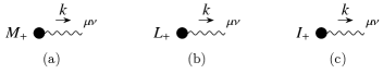
Figure 1: The Feynman diagrams needed for the computation $T_{+}^{\mu\nu}$ at leading order.

3.1 Failed tail & Memories

The failed-tail contribution is given by the diagrams (a) and (b) in Fig. 2. The derivation entails an integral of the form

$$T^{\mu\nu}_{+,(\textrm{FT})}(k)=\kappa^{2}L_{+}^{\alpha\beta}I_{+}^{\rho\sigma}(\omega)\int_{q}\frac{\delta\!\!\!{}^{-}(q^{0})\mathcal{N}^{(\rm FT)}_{\alpha\beta\rho\sigma}{}^{\mu\nu}(k,q,v,\eta)}{{\boldsymbol{q}}^{2}[(\omega+i0^{+})^{2}-|{\boldsymbol{k}}-{\boldsymbol{q}}|^{2}]}\,,$$ (3.3)

where we have already used that $L_{+}^{\alpha\beta}(q^{0})=L_{+}^{\alpha\beta}\delta\!\!\!{}^{-}(q^{0})+{\cal O}(G^{2})$. Using tensorial reduction and integration-by-parts (IBP) identities, we get

$$T^{\mu\nu}_{+\textrm{(FT)}}(k)=\kappa^{2}L_{+}^{\alpha\beta}I_{+}^{\rho\sigma}(\omega)\Big{[}\mathcal{N}^{({\rm FT}_{1})}_{\alpha\beta\rho\sigma}{}^{\mu\nu}(k,v,\eta){\cal I}^{(\rm FT)}_{0,1}+\mathcal{N}^{({\rm FT}_{2})}_{\alpha\beta\rho\sigma}{}^{\mu\nu}(k,v,\eta){\cal I}^{(\rm FT)}_{1,1}\Big{]}\,.$$ (3.4)

where we introduced the following family of master integrals

$${\cal I}^{\rm(FT)}_{ab}\equiv\int_{{\boldsymbol{q}}}\frac{1}{[{\boldsymbol{q}}^{2}]^{a}[(\omega+i0^{+})^{2}-|{\boldsymbol{k}}-{\boldsymbol{q}}|^{2}]^{b}}\,.$$ (3.5)

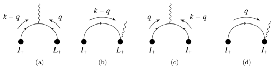
Figure 2: The Feynman diagrams needed for the NLO $T_{+}^{\mu\nu}$ in the physical limit. Diagrams (a) and (b) give the failed tail contribution, while (c) and (d) are responsible for the memory term. (We did not include the symmetric version of diagram (b), since it vanishes.)

Next we move to the computation of the memory contribution. This is obtained by computing the diagrams (c) and (d) of Fig. 2. Schematically, we find

$$T^{\mu\nu}_{+,(\textrm{M})}(k)=\kappa^{2}\int_{q}\frac{\mathcal{N}^{(\rm M)}_{\alpha\beta\rho\sigma}{}^{\mu\nu}(k,q,v,\eta)}{\big{[}(q^{0}+i0^{+})^{2}-|{\boldsymbol{k}}|^{2}\big{]}\big{[}(\omega-q^{0}+i0^{+})^{2}-|{\boldsymbol{k}}-{\boldsymbol{q}}|^{2}\big{]}}I_{+}^{\alpha\beta}(q^{0})I_{+}^{\rho\sigma}(\omega-q^{0})\,.$$ (3.6)

Through the use of IBP and tensorial reduction, this result can be simplified to

$$T^{\mu\nu}_{+\textrm{(M)}}(k)=\kappa^{2}\int\frac{{\mathrm{d}}q^{0}}{2\pi}I_{+}^{\rho\sigma}(q^{0})I_{+}^{\alpha\beta}(\omega-q^{0})\Big{[} \mathcal{N}^{({\rm M}_{1})}_{\alpha\beta\rho\sigma}{}^{\mu\nu}(k,q^{0},v,\eta)\mathcal{I}^{(\rm M)}_{1,0}+\mathcal{N}^{({\rm M}_{2})}_{\alpha\beta\rho\sigma}{}^{\mu\nu}(k,q^{0},v,\eta)\mathcal{I}^{(\rm M)}_{0,1}$$

$$+\mathcal{N}^{({\rm M}_{3})}_{\alpha\beta\rho\sigma}{}^{\mu\nu}(k,q^{0},v,\eta)\mathcal{I}^{(\rm M)}_{1,1}\Big{]}\,,$$ (3.7)

where, likewise, we have introduced the following family of master integrals

$$\mathcal{I}^{(\rm M)}_{ab}\equiv\int_{{\boldsymbol{q}}}\frac{1}{\big{[}(q^{0}+i0^{+})^{2}-|{\boldsymbol{k}}|^{2}\big{]}^{a}\big{[}(\omega-q^{0}+i0^{+})^{2}-|{\boldsymbol{k}}-{\boldsymbol{q}}|^{2}\big{]}^{b}}\,.$$ (3.8)

The explicit form of the stress-energy tensor, after adding up both contributions, is not particularly illuminating. We will use it shortly to derive the far-zone metric. Nevertheless, it is instructive to check the conservation laws, which we do next.

3.2 Ward identity

We now verify that the stress-energy tensor computed previously satisfies the Ward identities, $\partial_{\mu}T_{+}^{\mu\nu}(x)=0$, up to the order we are interested; or equivalently, in Fourier space,

$$\partial_{\mu}T_{+}^{\mu\nu}(x)=-i\int_{k}k_{\mu}T_{+}^{\mu\nu}(k)e^{-ik\cdot x}=0\,.$$ (3.9)

For the failed tail in (3.4) we readily find $k_{\nu}T^{\mu\nu}_{+\textrm{(FT)}}(k)=0$. Notice that, while the seagull-type (double-bubble) diagram in Fig.2(b) is not present in tail-type terms, it is crucial for the contribution from the failed tail to guarantee the conservation law. We are then left with the remaining combination

$$k_{\nu}\Big{(}T^{\mu\nu}_{+({\rm LO})}(k)+T^{\mu\nu}_{+\textrm{(M)}}(k)\Big{)}\,,$$ (3.10)

which includes the contributions from (3.1) and (3.7). After contracting with $k_{\mu}$, the result for the memory part greatly simplifies, using

$${\cal I}^{\rm(M)}_{1,0}=-\frac{i}{4\pi}q_{0}+{\cal O}(d-3)\,,\qquad{\cal I}^{\rm(M)}_{0,1}=-\frac{i}{4\pi}(w-q_{0})+{\cal O}(d-3)\,,$$ (3.11)

for the relevant integrals, we find

$$k_{\nu}T^{\mu\nu}_{+\textrm{(M)}}(k)=-i\frac{G}{5}\int\frac{{\mathrm{d}}q^{0}}{2\pi}\bigg{\{} q_{0}^{5}(\omega-q_{0})I^{\alpha\beta}(q_{0})I_{\alpha\beta}(\omega-q_{0})v^{\mu}$$

$$-\Big{[}\big{(}\omega-q_{0}\big{)}^{5}-q_{0}^{5}\Big{]}I^{\mu\alpha}(q_{0})I_{\alpha\beta}(\omega-q_{0})k^{\beta}\bigg{\}}\,,$$ (3.12)

where the first line only contributes to the $k_{\nu}T_{+}^{\nu 0}$ component, whereas the second goes into the spatial part. In coordinate space, this becomes

$$\partial_{\nu}T^{\nu\mu}_{+\textrm{(M)}}(x) =\frac{G}{5}\bigg{(}I^{(5)}_{ij}(t)I^{(1)}_{ij}(t)\delta^{\mu}_{0}\bigg{)}\delta^{3}({\boldsymbol{x}})+\frac{G\delta^{\mu}_{i}}{5}\bigg{(}{I}^{i}{}_{j}(t)I^{(5)}_{jk}(t)-{I^{(5)}}^{ij}(t)I_{jk}(t)\bigg{)}\partial_{k}\delta^{3}({\boldsymbol{x}})\,,$$ (3.13)

Hence, including the leading order result in (3.2), we arrive at

$$\partial_{\nu}T_{+}^{\nu 0}(x) =\left(\dot{M}(t)+\frac{G}{5}I^{(5)}_{ij}(t)I^{(1)}_{ij}(t)\right)\delta^{3}({\boldsymbol{x}})\,,$$ (3.14)

$$\partial_{\nu}T_{+}^{\nu}{}_{i}(x) =\left[\frac{1}{2}\dot{L}_{ik}(t)+\frac{G}{5}\bigg{(}I_{ij}(t)I^{(5)}_{jk}(t)-I^{(5)}_{ij}(t)I_{jk}(t)\bigg{)}\right]\partial_{k}\delta^{3}({\boldsymbol{x}})\,,$$

which vanishes upon using the (near-zone) conservation laws for the sources,

$$\dot{M}(t)=-\frac{G}{5}I^{(5)}_{ij}(t)I^{(1)}_{ij}(t)\,,\quad\par\dot{L}_{ij}(t)=-\frac{4G}{5}I_{k[i}(t)I^{(5)}_{j]k}(t)\,,$$ (3.15)

that follow from the leading order (in-in) effective action Galley:2015kus . The energy conservation agrees, as expected, with the result in Goldberger:2012kf , while the angular-momentum part extends it to the other components. Upon time averaging (i.e. up to Schott terms), we reproduce the known values (see, e.g., Eqs. (3.75) and (3.97) of Maggiore:2007ulw )

$$\langle\dot{M}(t)\rangle=-\frac{G}{5}\left\langle I^{ij(3)}(t)I^{ij(3)}(t)\right\rangle\,,\quad\langle\dot{{\boldsymbol{L}}}^{i}(t)\rangle=-\frac{2G}{5}\left\langle\varepsilon^{ijk}I^{lj(2)}(t)I^{lk(3)}(t)\right\rangle\,.$$ (3.16)

The above results are a direct consequence of invariance under diffeomorphisms. Let us point out, however, that the additional terms from the background-gauge condition did not feature in the Ward identity at this order. Yet, as we demonstrate in App. A, the (covariant) gauge fixing does play an important role in order to guarantee the conservation laws at higher orders.

3.3 GW fluxes

We compute now the radiated energy and angular momentum due to hereditary effects. We start by deriving the asymptotic waveform in transverse-traceless (TT) gauge,

$$h^{\textrm{TT}}_{ij}(x_{\rm ret})=\frac{\kappa}{8\pi r}\int\frac{{\mathrm{d}}\omega}{2\pi}e^{-i\omega t_{\rm ret}}f_{ij}(\omega,\omega{\boldsymbol{n}})\,,\qquad f_{ij}(\omega,\omega{\boldsymbol{n}})\equiv\Lambda_{ijab}T_{ab,+}(\omega,\omega{\boldsymbol{n}})\,,$$ (3.17)

where $x_{\rm ret}\equiv(t_{\rm ret},{\boldsymbol{x}})$, evaluated on the retarded time, and we introduced the normalized radial direction ${\boldsymbol{n}}$, with ${\boldsymbol{n}}\cdot{\boldsymbol{n}}=1$, and $\Lambda_{ijab}$ is given by

$$\Lambda_{ijab}=\mathbb{P}_{ia}\mathbb{P}_{jb}-\frac{1}{2}\mathbb{P}_{ij}\mathbb{P}_{ab}\,,\qquad\mathbb{P}_{ij}\equiv\delta_{ij}-n_{i}n_{j}\,,$$ (3.18)

which serves as a projector onto the TT gauge gauge. In what follows we drop the ‘ret’ label. From the asymptotic waveform, we compute the loss of energy and angular momentum (notice the overall minus signs)

$$\dot{M}(t) =-\lim_{r\to\infty}\int{\mathrm{d}}\Omega\,r^{2}\dot{h}^{\textrm{TT}}_{ij}\dot{h}^{\textrm{TT}}_{ij}\,,$$ (3.19)

$$\dot{L}_{ij}(t) =-\lim_{r\to\infty}\int{\mathrm{d}}\Omega\,r^{2}\left[2h^{\textrm{TT}}_{a[i}\dot{h}^{\textrm{TT}}_{j]a}-\dot{h}^{\textrm{TT}}_{ab}x_{[i}\partial_{j]}h^{\textrm{TT}}_{ab}\right]\,.$$ (3.20)

The waveform receives contributions at leading order, $f_{(0)}^{ij}(\omega)$, and from hereditary effects, $f_{\rm(H)}^{ij}(\omega)$, such that, for the energy flux we have

$$\dot{M}_{\rm(H)}(t) =\frac{\kappa^{2}}{32\pi^{2}}\int{\mathrm{d}}\Omega\int\frac{{\mathrm{d}}\omega_{1}{\mathrm{d}}\omega_{2}}{(2\pi)^{2}}e^{-i(\omega_{1}+\omega_{2})t}\omega_{1}\omega_{2}\Big{[}f_{(0)}^{ij}(\omega_{1})f_{\rm(H)}^{ij}(\omega_{2})\Big{]}\,.$$ (3.21)

whereas for the angular-momentum flux,

$$\dot{L}^{ij}_{\rm(H)}(t) =\frac{i\kappa^{2}}{64\pi^{2}}\int{\mathrm{d}}\Omega\frac{{\mathrm{d}}\omega_{1}{\mathrm{d}}\omega_{2}}{(2\pi)^{2}}e^{-i(\omega_{1}+\omega_{2})t}\big{(}\omega_{2}-\omega_{1}\big{)}\Big{[}2f_{(0)}^{l[i}(\omega_{1})f_{\rm(H)}^{j]l}(\omega_{2})-f_{\rm(H)}^{kl}(\omega_{2})n^{[i}\tilde{\partial}^{j]}f_{(0)}^{kl}(\omega_{1})\Big{]}\,,$$ (3.22)

where $x_{[i}\partial_{j]}=n_{[i}\mathbb{P}_{j]a}\tilde{\partial}{{}_{a}}$, with $\tilde{\partial}_{a}\equiv\partial/(\partial n^{a})$. Using the result given in (3.3), we then get the following contribution to the energy loss due to the failed-tail coupling,

$$\dot{M}_{\textrm{(FT)}}(t) =-\frac{2G^{2}}{15}L^{jk}\int\frac{{\mathrm{d}}\omega_{1}{\mathrm{d}}\omega_{2}}{(2\pi)^{2}}e^{-i(\omega_{1}+\omega_{2})t}I^{lj}(\omega_{1})I^{lk}(\omega_{2})\omega_{1}^{3}\omega_{2}^{5}$$

$$=-\frac{2G^{2}}{15}L^{jk}I^{(3)lj}(t)I^{(5)lk}(t)=0+\frac{{\mathrm{d}}}{{\mathrm{d}}t}\big{(}\cdots\big{)}\,.$$ (3.23)

which vanishes at this order. We omit the expression of the total derivative, which cancels out upon time averaging. For the memory part we find (with $\omega_{3}=\omega_{2}-q_{0}$)

$$\dot{M}_{\textrm{(M)}}(t) =\frac{2iG^{2}}{35}\int\frac{{\mathrm{d}}\omega_{1}{\mathrm{d}}\omega_{2}{\mathrm{d}}q_{0}}{(2\pi)^{3}}e^{-i(\omega_{1}+\omega_{2})t}I^{ij}(\omega_{1})I^{jk}(q_{0})I^{ki}(\omega_{3})\omega_{1}^{3}q_{0}^{3}\big{(}2\omega_{3}^{3}+11\omega_{3}^{2}q_{0}+14\omega_{3}q_{0}^{2}+7q_{0}^{3}\big{)}$$ (3.24)

$$=\frac{G^{2}}{5}I^{(1)ij}(t)I^{(4)jk}(t)I^{(4)ki}(t)+\frac{{\mathrm{d}}}{{\mathrm{d}}t}\big{(}\cdots\big{)}\,.$$

Following similar steps, the failed-tail contribution to the flux of angular momentum becomes

$$\dot{L}^{ij}_{\textrm{(FT)}}(t) =\frac{2G^{2}}{15}i\int\frac{{\mathrm{d}}\omega_{1}{\mathrm{d}}\omega_{2}}{(2\pi)^{2}}e^{-i(\omega_{1}+\omega_{2})t}\Big{(}I^{ki}(\omega_{1})I^{jl}(\omega_{2})L^{kl}+I^{kl}(\omega_{2})I^{k[i}(\omega_{1})L^{j]l}\Big{)}\omega_{1}^{2}(\omega_{1}-\omega_{2})\omega_{2}^{4}$$

$$=\frac{4G^{2}}{15}I^{(4)kl}(t)I^{(3)k[i}(t)L^{j]l}+\frac{{\mathrm{d}}}{{\mathrm{d}}t}\big{(}\cdots\big{)}\,.$$ (3.25)

There is an important difference for the memory part, which contains a term of the form

$$\dot{L}_{\rm nloc(M)}^{ij}(t) =\frac{8G^{2}}{35}\int\frac{{\mathrm{d}}\omega_{1}{\mathrm{d}}\omega_{2}{\mathrm{d}}\omega_{3}}{(2\pi)^{3}}e^{-i(\omega_{1}+\omega_{2})t}I^{k[i}(\omega_{1})I^{j]l}(q_{0})I^{kl}(\omega_{3})\bigg{[}\frac{\omega_{1}^{3}q_{0}^{6}}{\omega_{2}+i0^{+}}\bigg{]}\,,$$ (3.26)

responsible for nonlocal-in-time effects in the flux. This can be seen by rewriting it as

$$\dot{L}_{{\rm nloc(M)}}^{ij}(t)=\frac{8G^{2}}{35} \int{\mathrm{d}}\tau I^{(3)k[i}(t)I^{(6)j]b}(\tau)I^{kl}(\tau)\int\frac{{\mathrm{d}}\omega_{2}}{2\pi}\frac{ie^{i\omega_{2}(\tau-t)}}{\omega_{2}+i0^{+}}\,,$$ (3.27)

and using

$$i\int\frac{{\mathrm{d}}\omega_{2}}{2\pi}\frac{e^{i\omega_{2}(t_{3}-t)}}{\omega_{2}+i0^{+}}=\vartheta(t-t_{3})\,,$$ (3.28)

such that

$$\dot{L}_{\rm nloc(M)}^{ij}(t)=\frac{8G^{2}}{35}I^{(3)k[i}(t)\int_{-\infty}^{t}{\mathrm{d}}\tau\,I^{(6)j]l}(\tau)I^{kl}(\tau)\,,$$ (3.29)

which agrees with the known nonlocal-in-time contribution (see e.g. Eq. (2.8) in Bini:2021qvf ). Combining the pieces, we find

$$\dot{L}^{ij}_{\rm(M)}(t)= -\frac{4G^{2}}{5}I^{(4)a[i}(t)I^{j]b}(t)I^{(4)ab}(t)-\frac{8G^{2}}{35}I^{(2)a[i}(t)I^{(3)j]b}(t)I^{(3)ab}(t)$$

$$-\frac{8G^{2}}{35}I^{(3)a[i}(t)\int_{-\infty}^{t}{\mathrm{d}}\tau\,I^{(3)j]b}(\tau)I^{(3)ab}(\tau)+\frac{{\mathrm{d}}}{{\mathrm{d}}t}\big{(}\cdots\big{)}\,,$$ (3.30)

where the last total derivative involves only local-in-time terms which vanish at infinity.For the sake of comparison with the literature, e.g. Arun:2009mc , it is instructive to compute an averaged value by integrating over the binary’s history divided by $T$, the elapsed time, and take the $T\to\infty$ limit. For the nonlocal-in-time part we find

$$\langle\dot{L}^{ij}_{\rm nloc(M)}(t)\rangle \equiv\lim_{T\to\infty}\frac{1}{T}\int{\mathrm{d}}t\dot{L}^{ij}_{\rm nloc(M)}(t)$$ (3.31)

$$=\frac{8G^{2}}{35T}\int\frac{{\mathrm{d}}\omega_{1}{\mathrm{d}}\omega_{2}{\mathrm{d}}q_{0}}{(2\pi)^{3}}\delta\!\!\!{}^{-}(\omega_{1}+\omega_{2})\bigg{[}\frac{\omega_{1}^{3}q_{0}^{6}}{\omega_{2}+i0^{+}}\bigg{]}I^{a[i}(\omega_{1})I^{j]b}(q_{0})I^{ab}(\omega_{2}-q_{0})\,.$$

Naively, one would be tempted to solve the $\delta(\omega_{1}+\omega_{2})$ and simply cancel a factor of $\tfrac{\omega_{1}}{\omega_{2}+i0^{+}}$. However, that would be incorrect since that ignores the $\omega_{2}\to 0$ soft-frequency limit, for which the $i0^{+}$-prescription becomes important. Using the distribution identity

$$\frac{1}{\omega_{2}+i0^{+}}=\frac{\mathscr{P}}{\omega_{2}}-\frac{i}{2}\delta\!\!\!{}^{-}(\omega_{2})\,,$$ (3.32)

then (3.31) can be split into two terms

$$\langle\dot{L}^{ij}_{\rm nloc(M)}(t)\rangle=\langle\dot{L}^{ij}_{\rm nloc(M)}(t)\rangle_{\mathscr{P}}+\langle\dot{L}^{ij}_{\rm nloc(M)}(t)\rangle_{\delta}.$$ (3.33)

One the one hand, using the distributional identity $\omega\mathscr{P}(1/\omega)=1$, the part of the principal value renormalizes the local-in-time contribution adding up to the total value

$$\langle\dot{L}^{ij}_{\rm loc(M)}(t)\rangle =-\frac{i}{T}\frac{4G^{2}}{35}\int\frac{{\mathrm{d}}\omega_{1}{\mathrm{d}}\omega_{2}{\mathrm{d}}q_{0}}{(2\pi)^{3}}I^{a[i}(\omega_{1})I^{j]b}(q_{0})I^{ab}(\omega_{2}-q_{0})\omega_{1}^{3}q_{0}^{6}\delta\!\!\!{}^{-}(\omega_{1}+\omega_{2})\delta\!\!\!{}^{-}(\omega_{2})\,$$

$$=-\frac{4G^{2}}{5}\left\langle I^{(4)a[i}(t)I^{j]b}(t)I^{(4)ab}(t)\right\rangle\,.$$ (3.34)

On the other hand, the nonlocal-in-time part involving the zero-frequency limit yields

$$\langle\dot{L}^{ij}_{\textrm{nloc(M)}}(t)\rangle_{\delta} =-i\frac{4G^{2}}{35T}\int\frac{{\mathrm{d}}\omega_{1}}{2\pi}\delta\!\!\!{}^{-}(\omega_{1})\omega_{1}^{3}I^{a[i}(\omega_{1})\int\frac{{\mathrm{d}}q_{0}}{2\pi}I^{j]b}(q_{0})I^{ab}(-q_{0})q_{0}^{6}$$

$$=-\frac{4G^{2}}{35}\left\langle I^{(3)a[i}(t)\right\rangle\int{\mathrm{d}}\tau I^{(3)j]b}(\tau)I^{(3)ab}(\tau)\,.$$ (3.35)

This results then agrees with the value in Arun:2009mc , where the nonlocal-in-time term is associated with a so-called ‘DC’ memory contribution, see e.g. the first part of Eq. (5.14) in Arun:2009mc , and notice that the factor of $1/2$ in (3.32) accounts for the half integration over the energy flux.

4 Radiative action

In order to obtain the form of the radiation-reaction forces upon the binary’s dynamics, we compute the total (in-in) effective action by integrating over the $\bar{h}_{\pm}$ field. We perform the computation for the failed-tail and memory contributions in what follows.

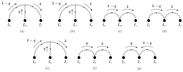
Figure 3: Feynman diagrams contributing to the in-in effective action. Diagrams (a) to (d) enter in the failed tail, whereas the memory is given by the sum of diagrams (e), (f) and (g).

4.1 Failed tail

The failed tail is given by the diagrams in Figs. 3(a) to 3(d). After various manipulations, including tensorial reduction and IBP relations, we find

$$S_{(\textrm{FT})}^{\textrm{(a)}\&\textrm{(c)}} =+\frac{1}{15}\frac{i\kappa^{4}}{64}\int\frac{{\mathrm{d}}\omega{\mathrm{d}}q_{0}}{(2\pi)^{2}}L_{+}^{kl}(q_{0})I_{-}^{ik}(-\omega)I_{+}^{li}(\omega-q_{0})\omega^{5}\mathcal{I}_{(\textrm{FT})+}(\omega)\,,$$ (4.1)

$$S_{(\textrm{FT})}^{\textrm{(b)}\&\textrm{(d)}} =-\frac{1}{15}\frac{i\kappa^{4}}{128}\int\frac{{\mathrm{d}}\omega{\mathrm{d}}q_{0}}{(2\pi)^{2}}L_{-}^{kl}(q_{0})I_{+}^{ik}(\omega-q_{0})I_{+}^{li}(-\omega)\omega^{5}\mathcal{I}_{(\textrm{FT})-}(\omega)\,,$$ (4.2)

where it is understood that, at this order, $L_{+}^{kl}(q_{0})=L_{+}^{kl}\delta\!\!\!{}^{-}(q_{0})$. For this reason, the final result is really just a function of one frequency $\omega$. The two relevant master integrals, $\mathcal{I}_{(\textrm{FT})\pm}(\omega)$, are straightforward to compute,

$$\mathcal{I}_{(\textrm{FT})\pm}(\omega)=\int_{{\boldsymbol{k}}}\frac{1}{(\omega\pm i0^{+})^{2}-{\boldsymbol{k}}^{2}}\int_{{\boldsymbol{q}}}\frac{1}{(\omega+i0^{+})^{2}-{\boldsymbol{q}}^{2}}=\mp\frac{\omega^{2}}{16\pi^{2}}+O(d-3)\,.$$ (4.3)

After Fourier transforming to coordinate space, we have

$$S_{(\textrm{FT})} =-\frac{G^{2}}{15}\int\!{\mathrm{d}}t\,L_{+}^{kl}I^{(4)}_{-,kj}I^{(3)}_{+,jl}+\frac{G^{2}}{30}\int\!{\mathrm{d}}t\,L_{-}^{kl}I^{(4)}_{+,kj}I^{(3)}_{+,jl}\,.$$ (4.4)

Notice that, unlike tail terms, e.g. Galley:2015kus , the failed-tail contribution is finite in $d=3$.The first term in (4.4) agrees with the result in Almeida:2023yia . On the other hand, the term proportional to $L^{ij}_{-}$ was not included. As we shall see in §4.4, this extra term is crucial to recover the flux of angular momentum derived in (3.25).

4.2 Memories

The memory contribution is given by adding Figs. 3(e), 3(f) and 3(g). While the computation of the last two diagrams is straightforward, the Feynman integral in 3(e) turns out to be subtle, depending on the following family of master integrals

$${\cal I}_{abc}\equiv\int_{{\boldsymbol{q}},{\boldsymbol{k}}}\frac{1}{[(\omega_{1}+i0^{+})^{2}-{\boldsymbol{q}}^{2}]^{a}[(\omega_{2}+i0^{+})^{2}-|{\boldsymbol{k}}+{\boldsymbol{q}}|^{2}]^{b}[(\omega_{3}+i0^{+})^{2}-{\boldsymbol{k}}^{2}]^{c}}\,,$$ (4.5)

such that

$$S_{\rm(M)}^{\rm(e)}=\kappa^{4} \int\frac{{\mathrm{d}}\omega_{1}{\mathrm{d}}\omega_{2}{\mathrm{d}}\omega_{3}}{(2\pi)^{3}}\delta\!\!\!{}^{-}(\omega_{1}+\omega_{2}-\omega_{3})I_{-}^{ij}(-\omega_{3})I_{+}^{jk}(\omega_{1})I_{+}^{ki}(\omega_{2})\bigg{[}c_{1}{\cal I}_{110}+c_{2}{\cal I}_{101}+c_{3}{\cal I}_{011}+c_{4}{\cal I}_{111}\bigg{]}\,,$$ (4.6)

where the $c_{i}$’s are functions of $\omega_{1,2,3}$. While the other diagrams in Figs. 3(f) and 3(g) only depend on the ${\cal I}_{110}$, ${\cal I}_{101}$ and ${\cal I}_{011}$ masters, which are straightforward to compute, i.e.

$${\cal I}_{110} =-\frac{\omega_{1}\omega_{2}}{16\pi^{2}}+{\cal O}(d-3)\,,\,\,{\cal I}_{101}=-\frac{\omega_{1}\omega_{3}}{16\pi^{2}}+{\cal O}(d-3)\,,\,\,{\cal I}_{011}=-\frac{\omega_{2}\omega_{3}}{16\pi^{2}}+{\cal O}(d-3)\,,$$ (4.7)

the expression in (4.6) depends also on ${\cal I}_{111}$, which a priori entails three different frequencies. Naively, due to the overall $\delta$-function, one would be tempted to replace $\omega_{1}+\omega_{2}-\omega_{3}=0$, in which case ${\cal I}_{111}$ reduces through IBP relations into a combination of the ones in (4.7). Furthermore, although divergent ($\propto 1/(d-3)$), the ${\cal I}_{111}$ enters through a term proportional to $(\omega_{1}+\omega_{2}-\omega_{3})^{2}$, dropping out of the final (finite) answer. This was the route ultimately taken in the derivations in Foffa:2019eeb ; Blumlein:2021txe ; Almeida:2022jrv . Even though this procedure correctly recovers the local-in-time part, it does not fully account for all the relevant terms. In particular, it fails to reproduce the correct nonlocal-in-time flux of angular momentum. That is because the master integral in ${\cal I}_{111}$ cannot be ignored, since it contributes in the limit in which all the frequencies go to zero ${\omega_{i}\to 0}$ yielding, as we shall see, a nonlocal-in-time boundary term. We discuss all the relevant memory corrections below.

4.2.1 Local-in-time

For the local-in-time part of the memory we follow the procedure in Blumlein:2021txe ; Almeida:2022jrv (but with the corrected Feynman rules), and ignore the contribution from ${\cal I}_{111}$. We find ($\omega_{2}\equiv\omega_{3}-\omega_{1}$),

$$S^{\textrm{(e)}}_{\rm loc\textrm{(M)}} =\frac{G^{2}}{35}\int\frac{{\mathrm{d}}\omega_{3}{\mathrm{d}}\omega_{1}}{(2\pi)^{2}}I_{-}^{ij}(-\omega_{3})I_{+}^{jk}(\omega_{1})I_{+}^{ki}(\omega_{2})\bigg{[}\omega_{1}^{2}\omega_{2}^{2}\left(\omega_{1}^{4}+10\omega_{1}^{3}\omega_{2}+25\omega_{1}^{2}\omega_{2}^{2}+10\omega_{1}\omega_{2}^{3}+\omega_{2}^{4}\right)$$

$$\qquad-2\omega_{3}^{2}\omega_{1}^{2}\left(\omega_{3}^{4}-10\omega_{3}^{3}\omega_{1}+25\omega_{3}^{2}\omega_{1}^{2}-10\omega_{3}\omega_{1}^{3}+\omega_{1}^{4}\right)\bigg{]}\,,$$ (4.8)

$$S^{\textrm{(f)\&(g)}}_{\textrm{(M)}} =-\frac{G^{2}}{5}\int\frac{{\mathrm{d}}\omega_{3}{\mathrm{d}}\omega_{1}}{(2\pi)^{2}}I_{-}^{ij}(-\omega_{3})I_{+}^{jk}(\omega_{1})I_{+}^{ki}(\omega_{2})\omega_{1}^{3}\left[2\omega_{3}^{5}-5\omega_{3}^{4}\omega_{1}+2\omega_{3}^{3}\omega_{1}^{2}\right.$$

$$\qquad+\left.\frac{\omega_{2}^{3}}{2}\big{(}2\omega_{1}^{2}+5\omega_{1}\omega_{2}+2\omega_{2}^{2}\big{)}\right]\,.$$ (4.9)

Up to total time derivatives, these can be rewritten as

$$S^{\textrm{(e)}}_{\rm loc\textrm{(M)}} =\frac{G^{2}}{5}\int{\mathrm{d}}t\left[I_{-,ij}I^{(4)}_{+,jk}I^{(4)}_{+,ki}-2I^{(4)}_{-,ij}I^{(4)}_{+,jk}I_{+,ki}+\frac{8}{7}I^{(2)}_{-,ij}I^{(3)}_{+,jk}I^{(3)}_{+,ki}-\frac{12}{7}I^{(3)}_{-,ij}I^{(3)}_{+,jk}I^{(2)}_{+,ki}\right]\,,$$ (4.10)

$$S^{\textrm{(f)\&(g)}}_{\textrm{(M)}} =\frac{G^{2}}{5}\int{\mathrm{d}}t\left[I^{(4)}_{-,ij}I^{(4)}_{+,jk}I_{+,ki}-\frac{1}{2}I_{-,ij}I^{(4)}_{+,jk}I^{(4)}_{+,ki}-I^{(2)}_{-,ij}I^{(3)}_{+,jk}I^{(3)}_{+,ki}+2I^{(3)}_{-,ij}I^{(3)}_{+,jk}I^{(2)}_{+,ki}\right]\,.$$ (4.11)

While the result in (4.10) agrees with the previous computations in Blumlein:2021txe ; Almeida:2022jrv , the result in (4.11) fails to match the double-bubble contribution(s). Putting both terms together, we finally arrive at

$$S_{\rm loc\textrm{(M)}}=\frac{G^{2}}{5}\int{\mathrm{d}}t\left[\frac{1}{2}I_{-,ij}I^{(4)}_{+,jk}I^{(4)}_{+,ki}-I^{(4)}_{-,ij}I^{(4)}_{+,jk}I_{+,ki}+\frac{1}{7}I^{(2)}_{-,ij}I^{(3)}_{+,jk}I^{(3)}_{+,ki}+\frac{2}{7}I^{(3)}_{-,ij}I^{(3)}_{+,jk}I^{(2)}_{+,ki}\right]\,.$$ (4.12)

4.2.2 Soft-frequency limit

In order to capture the soft-frequency limit (SFL) contribution to the memory diagram in 3(e), it is instructive to rederive the integrand in terms of the stress-energy tensor, prior to integrating over the $\bar{h}_{\pm}$ field(s), which can be split as (see also Almeida:2023yia for the case of tail terms)

$$\textrm{Fig}.\,\ref{Fig:Sinin}{\rm(e)} =\int\frac{{\mathrm{d}}\omega_{1}{\mathrm{d}}\omega_{2}{\mathrm{d}}\omega_{3}}{(2\pi)^{3}}\delta\!\!\!{}^{-}(\omega_{1}+\omega_{2}+\omega_{3})$$

$$\int_{{\boldsymbol{k}}}\bigg{[}\frac{-i\kappa}{2}\leavevmode\hbox to0pt{\vbox to0pt{\text{[drawing]}}}\bigg{]}^{\mu\nu}\frac{iP_{\mu\nu\rho\sigma}}{(\omega_{1}+\omega_{2}+i0^{+})^{2}-{\boldsymbol{k}}^{2}}\bigg{[}\frac{-i\kappa}{2}\leavevmode\hbox to0pt{\vbox to0pt{\text{[drawing]}}}\bigg{]}^{\rho\sigma}+{\rm perms.}\,, {\scriptstyle I_{+}(\omega_{1})} {\scriptstyle I_{+}(\omega_{2})} {\scriptstyle(\omega_{1}+\omega_{2}\text{,}{\boldsymbol{k}})} {\scriptstyle I_{-}(\omega_{3})} {\scriptstyle(\omega_{3}\text{,}{\boldsymbol{k}})} {\scriptstyle I_{+}(\omega_{1})} {\scriptstyle I_{+}(\omega_{2})} {\scriptstyle(\omega_{1}+\omega_{2}\text{,}{\boldsymbol{k}})} {\scriptstyle I_{-}(\omega_{3})} {\scriptstyle(\omega_{3}\text{,}{\boldsymbol{k}})}$$ (4.13)

where the permutations account for the various possible cuts of the would-be ${\cal I}_{111}$ (modulo the proper symmetry factors). Moreover, since the soft limit is dominated by three radiation modes, we can further consider the associated cut propagators to be on-shell, which greatly simplifies the computation. Let us start with the first term displayed in (4.2.2) and consider the limit $\omega_{1}+\omega_{2}\to 0$, for which we get

$$\bigg{[}\lim_{\omega_{1}+\omega_{2}\to 0}\leavevmode\hbox to0pt{\vbox to0pt{\text{[drawing]}}}\bigg{]}^{\mu\nu}=\frac{1}{\omega_{1}+\omega_{2}+i0^{+}}T^{\mu\nu}_{\textrm{SFL(M)}}(\omega_{1}+\omega_{2},{\boldsymbol{k}})\,. {\scriptstyle I_{+}(\omega_{1})} {\scriptstyle I_{+}(\omega_{2})} {\scriptstyle(\omega_{1}+\omega_{2}\text{,}{\boldsymbol{k}})} {\scriptstyle I_{+}(\omega_{1})} {\scriptstyle I_{+}(\omega_{2})} {\scriptstyle(\omega_{1}+\omega_{2}\text{,}{\boldsymbol{k}})}$$ (4.14)

such that,

$$\textrm{Fig}.\,\ref{Fig:Sinin}{\rm(e)}\bigg{|}_{\omega_{1}+\omega_{2}\to 0} =-i\frac{\kappa^{2}}{4}\int\frac{{\mathrm{d}}\omega_{1}{\mathrm{d}}\omega_{2}{\mathrm{d}}\omega_{3}}{(2\pi)^{3}}\delta\!\!\!{}^{-}(\omega_{1}+\omega_{2}+\omega_{3})\frac{1}{\omega_{1}+\omega_{2}+i0^{+}}$$

$$\times\int_{\boldsymbol{k}}T^{\mu\nu}_{+\textrm{SFL(M)}}(\omega_{1}+\omega_{2},{\boldsymbol{k}})\frac{P_{\mu\nu\rho\sigma}}{(-\omega_{3}+i0^{+})^{2}-{\boldsymbol{k}}^{2}}T_{-,(LO)}^{\rho\sigma}(\omega_{3},{\boldsymbol{k}})\,.$$ (4.15)

After tensorial reduction, and solving the integral over ${\boldsymbol{k}}$, we find

$$\textrm{Fig}.\,\ref{Fig:Sinin}{\rm(e)}\bigg{|}_{\omega_{1}+\omega_{2}\to 0}=i\frac{2G^{2}}{35}\int\frac{{\mathrm{d}}\omega_{1}{\mathrm{d}}\omega_{2}{\mathrm{d}}\omega_{3}}{(2\pi)^{3}}I_{+}^{ij}(\omega_{1})I_{+}^{jk}(\omega_{2})I_{-}^{ki}(\omega_{3})\frac{\omega_{3}^{3}\omega_{1}^{6}}{\omega_{1}+\omega_{2}+i0^{+}}\delta\!\!\!{}^{-}(\omega_{1}+\omega_{2}+\omega_{3})\,.$$ (4.16)

Hence, using the distributional identity in (3.32), and keeping only the nonlocal-in-time term, in which all the frequencies go to zero, we arrive at

$$\textrm{Fig}.\,\ref{Fig:Sinin}{\rm(e)}\bigg{|}_{\omega_{1}+\omega_{2}\to 0,\omega_{3}\to 0}=\frac{G^{2}}{35}\int\frac{{\mathrm{d}}\omega_{1}{\mathrm{d}}\omega_{2}{\mathrm{d}}\omega_{3}}{(2\pi)^{3}}\omega_{1}^{6}\omega_{3}^{3}\delta\!\!\!{}^{-}(\omega_{1}+\omega_{2})\delta\!\!\!{}^{-}(\omega_{1}+\omega_{2}+\omega_{3})I_{+}^{ij}(\omega_{1})I_{+}^{jk}(\omega_{2})I_{-}^{ki}(\omega_{3})\,.$$ (4.17)

The contribution from the other cuts involves the coupling of $T^{\mu\nu}_{+\rm(LO)}$ with $T^{\mu\nu}_{-\rm SFL(M)}$ instead. However, since the diagram turns out to be proportional to two terms (with retarded and advanced propagators) of opposite signs, we find that the latter vanishes in the soft-frequency limit. Hence, we arrive at the final result

$$S_{\rm nloc(M)}=-i\frac{G^{2}}{35}\bigg{[} \int\frac{{\mathrm{d}}\omega_{1}{\mathrm{d}}\omega_{3}}{(2\pi)^{2}}\delta\!\!\!{}^{-}(\omega_{3})\omega_{3}^{3}I_{-}^{ij}(\omega_{3})\omega_{1}^{6}I_{+}^{jk}(-\omega_{1})I_{+}^{ki}(\omega_{1})\bigg{]}\,,$$ (4.18)

proportional to $\omega^{3}\delta(\omega)I^{ij}(\omega)$. It is somewhat instructive to regroup some of the terms together, and rewrite the entire contribution from the soft-frequency limit as follows

$$S_{\textrm{SFL(M)}}=-\frac{2G^{2}}{35}\int\!\!{\mathrm{d}}t\bigg{[}I_{+}^{(6)ij}(t)I_{+}^{jk}(t)I_{-}^{(2)ki}(t)-\frac{{\mathrm{d}}}{{\mathrm{d}}t}\bigg{\{}I_{-}^{(2)ij}(t)\int{\mathrm{d}}\tau\vartheta(t-\tau)I_{+}^{(6)jk}(\tau)I_{+}^{ki}(\tau)\bigg{\}}\bigg{]}\,,$$ (4.19)

after absorbing the associated local-in-time contribution. Notice, as anticipated, the nonlocal-in-time part becomes a total time derivative, hence a boundary term in the action.

4.3 Radiation-reaction forces

The total in-in effective action, including radiative effects, takes the general form,

$$S[{\boldsymbol{x}}_{\pm}]=\int{\mathrm{d}}t\Big{(}\mathcal{L}+R_{\pm}\Big{)}\,,$$ (4.20)

where $\mathcal{L}$ is a conservative-like Lagrangian, including the kinetic and potential-only terms computed to 5PN order in Blumlein:2020pyo , as well as other conservative-like tail terms, e.g. Galley:2015kus ; Almeida:2021xwn . On the other hand, the $R_{\pm}$ part accounts for various radiation-reaction effects, starting with the leading (Burke-Thorne) radiation-reaction action Galley:2015kus

$$S_{\rm(RR)}=-\frac{G}{5}\int{\mathrm{d}}t\,I^{ij}_{-}(t)I^{ij(5)}_{+}(t)\,.$$ (4.21)

The equation of motion are then given by Galley:2009px

$$\frac{{\mathrm{d}}}{{\mathrm{d}}t}\frac{\partial\mathcal{L}}{\partial{\boldsymbol{v}}^{i}_{a}}-\frac{\partial\mathcal{L}}{\partial{\boldsymbol{x}}^{i}_{a}}=\bigg{[}\frac{\partial R_{\pm}}{\partial{\boldsymbol{x}}^{i}_{a,-}}-\frac{{\mathrm{d}}}{{\mathrm{d}}t}\frac{\partial R_{\pm}}{\partial{\boldsymbol{v}}^{i}_{a,-}}\bigg{]}\bigg{|}_{\textrm{PL}}\,,$$ (4.22)

where PL stands for “Physical Limit”, i.e., ${\boldsymbol{x}}_{a,+}\to{\boldsymbol{x}}_{a}$, ${\boldsymbol{x}}_{a,-}\to 0$.At this stage we treat the full failed-tail and memory contributions as part of the radiative sector, and discuss their conservative-like counterparts shortly. Since the nonlocal-in-time contribution in (4.19) depends on the value of $\ddot{I}_{-}^{ij}$ at the boundaries, it does not contribute to the (Lagrangian) mechanics of the system (see below). Hence, using (4.22) we obtain

$${\boldsymbol{a}}_{(\textrm{FT})} =\frac{G^{3}M^{3}\nu^{2}}{r^{4}}\bigg{[}\bigg{(}36v^{6}-288v^{4}({\boldsymbol{v}}\cdot{\boldsymbol{n}})^{2}+112v^{2}({\boldsymbol{v}}\cdot{\boldsymbol{n}})^{4}+252({\boldsymbol{v}}\cdot{\boldsymbol{n}})^{6}\bigg{)}{\boldsymbol{n}}$$

$$\qquad\qquad-\bigg{(}84v^{4}({\boldsymbol{v}}\cdot{\boldsymbol{n}})-588v^{2}({\boldsymbol{v}}\cdot{\boldsymbol{n}})^{3}+616({\boldsymbol{v}}\cdot{\boldsymbol{n}})^{5}\bigg{)}{\boldsymbol{v}}\bigg{]}$$

$$-\frac{4G^{4}M^{4}\nu^{2}}{5r^{5}}\bigg{[}\bigg{(}47v^{4}+163v^{2}({\boldsymbol{v}}\cdot{\boldsymbol{n}})^{2}-630({\boldsymbol{v}}\cdot{\boldsymbol{n}})^{4}\bigg{)}{\boldsymbol{n}}-\bigg{(}350v^{2}({\boldsymbol{v}}\cdot{\boldsymbol{n}})-770({\boldsymbol{v}}\cdot{\boldsymbol{n}})^{3}\bigg{)}{\boldsymbol{v}}\bigg{]}$$

$$+\frac{8G^{5}M^{5}\nu^{2}}{15r^{6}}\bigg{[}\bigg{(}11v^{2}+199({\boldsymbol{v}}\cdot{\boldsymbol{n}})^{2}\bigg{)}{\boldsymbol{n}}-210({\boldsymbol{v}}\cdot{\boldsymbol{n}}){\boldsymbol{v}}\bigg{]}\,,$$ (4.23)

$${\boldsymbol{a}}_{(\textrm{M})} =-\frac{2G^{3}M^{3}\nu^{2}}{35r^{4}}\bigg{[}\bigg{(}2484v^{6}-38325v^{4}({\boldsymbol{v}}\cdot{\boldsymbol{n}})^{2}+91770v^{2}({\boldsymbol{v}}\cdot{\boldsymbol{n}})^{4}-56385({\boldsymbol{v}}\cdot{\boldsymbol{n}})^{6}\bigg{)}{\boldsymbol{n}}$$

$$\qquad\qquad+\bigg{(}9633v^{4}({\boldsymbol{v}}\cdot{\boldsymbol{n}})-33870v^{2}({\boldsymbol{v}}\cdot{\boldsymbol{n}})^{3}+24885({\boldsymbol{v}}\cdot{\boldsymbol{n}})^{5}\bigg{)}{\boldsymbol{v}}\bigg{]}$$

$$+\frac{4G^{4}M^{4}\nu^{2}}{315r^{5}}\bigg{[}\bigg{(}13900v^{4}-95892v^{2}({\boldsymbol{v}}\cdot{\boldsymbol{n}})^{2}+76680({\boldsymbol{v}}\cdot{\boldsymbol{n}})^{4}\bigg{)}{\boldsymbol{n}}$$

$$\hskip 56.9055pt+\bigg{(}32163v^{2}({\boldsymbol{v}}\cdot{\boldsymbol{n}})-35955({\boldsymbol{v}}\cdot{\boldsymbol{n}})^{3}\bigg{)}{\boldsymbol{v}}\bigg{]}$$

$$-\frac{16G^{5}M^{5}\nu^{2}}{1260r^{6}}\bigg{[}\bigg{(}2028v^{2}+9421({\boldsymbol{v}}\cdot{\boldsymbol{n}})^{2}\bigg{)}{\boldsymbol{n}}-393({\boldsymbol{v}}\cdot{\boldsymbol{n}}){\boldsymbol{v}}\bigg{]}-\frac{824G^{6}M^{6}\nu^{2}}{63r^{7}}{\boldsymbol{n}}\,,$$ (4.24)

for the relative acceleration(s), ${\boldsymbol{a}}\equiv{\boldsymbol{a}}_{1}-{\boldsymbol{a}}_{2}$, with $M=m_{1}+m_{2}$, $\nu=\frac{m_{1}m_{2}}{M^{2}}$, ${\boldsymbol{r}}\equiv{\boldsymbol{x}}_{1}-{\boldsymbol{x}}_{2}$, ${\boldsymbol{v}}\equiv{\boldsymbol{v}}_{1}-{\boldsymbol{v}}_{2}$. Since these will be useful later on, we also quote the Burke-Thorne radiation-reaction force, both after inputing the Newtonian acceleration,

$${\boldsymbol{a}}_{\rm(N)}=-GM\frac{{\boldsymbol{r}}}{r^{3}}\,,$$ (4.25)

at linear order,

$${\boldsymbol{a}}_{\rm(RR)} =\frac{8G^{2}M^{2}\nu}{5r^{3}}\bigg{[}\bigg{(}18v^{2}-25({\boldsymbol{v}}\cdot{\boldsymbol{n}})^{2}\bigg{)}({\boldsymbol{v}}\cdot{\boldsymbol{n}}){\boldsymbol{n}}-\bigg{(}6v^{2}-15({\boldsymbol{v}}\cdot{\boldsymbol{n}})^{2}\bigg{)}{\boldsymbol{v}}\bigg{]}+$$

$$\hskip 56.9055pt+\frac{16G^{3}M^{3}\nu}{5r^{4}}\bigg{[}{\boldsymbol{v}}+\frac{{\boldsymbol{v}}\cdot{\boldsymbol{n}}}{3}{\boldsymbol{n}}\bigg{]}\,,$$ (4.26)

and at second order, after plugging it back onto itself,

$${\boldsymbol{a}}_{\rm(RR^{2})} =\frac{16G^{3}M^{3}\nu^{2}}{5r^{4}}\bigg{[}\bigg{(}168v^{6}-3465({\boldsymbol{v}}\cdot{\boldsymbol{n}})^{6}-2496v^{4}({\boldsymbol{v}}\cdot{\boldsymbol{n}})^{2}+5789v^{2}({\boldsymbol{v}}\cdot{\boldsymbol{n}})^{4}\bigg{)}{\boldsymbol{n}}$$ (4.27)

$$\hskip 56.9055pt+\bigg{(}738v^{4}+1715({\boldsymbol{v}}\cdot{\boldsymbol{n}})^{4}-2449v^{2}({\boldsymbol{v}}\cdot{\boldsymbol{n}})^{2}\bigg{)}({\boldsymbol{v}}\cdot{\boldsymbol{n}}){\boldsymbol{v}}\bigg{]}$$

$$-\frac{32G^{4}M^{4}\nu^{2}}{225r^{5}}\bigg{[}\bigg{(}3898v^{4}-28131v^{2}({\boldsymbol{v}}\cdot{\boldsymbol{n}})^{2}+22755({\boldsymbol{v}}\cdot{\boldsymbol{n}})^{4}\bigg{)}{\boldsymbol{n}}$$

$$\hskip 56.9055pt+6\bigg{(}1921v^{2}-1830({\boldsymbol{v}}\cdot{\boldsymbol{n}})^{2}\bigg{)}({\boldsymbol{v}}\cdot{\boldsymbol{n}}){\boldsymbol{v}}\bigg{]}$$

$$+\frac{64G^{5}M^{5}\nu^{2}}{225r^{6}}\bigg{[}\bigg{(}311v^{2}+689({\boldsymbol{v}}\cdot{\boldsymbol{n}})^{2}\bigg{)}{\boldsymbol{n}}-234({\boldsymbol{v}}\cdot{\boldsymbol{n}}){\boldsymbol{v}}\bigg{]}+\frac{1792G^{6}M^{6}\nu^{2}}{75r^{7}}{\boldsymbol{n}}\,.$$

4.4 Near-zone dissipation

We are now in position to check that the near-zone dynamics is consistent with the radiated energy and angular momentum computed from the metric perturbation at infinity. Because of the subtleties with the extra boundary term in the action, we split the discussion into local- and nonlocal-in-time terms.

4.4.1 Local-in-time

We start by constructing the energy and angular momentum of the two-body system through the (local-in-time) conservative part of the action,

$$M\equiv\sum_{a=1,2}{\boldsymbol{v}}_{a}\cdot\frac{\partial\mathcal{L}}{\partial{\boldsymbol{v}}_{a}}-\mathcal{L}\,,\qquad\frac{1}{2}L^{ij}\equiv\sum_{a=1,2}{\boldsymbol{x}}_{a}^{[i}\frac{\partial\mathcal{L}}{\partial{\boldsymbol{v}}_{a}^{j]}}\,,$$ (4.28)

such that the Euler-Lagrangian equations imply

$$\dot{M} =\sum_{a}{\boldsymbol{v}}_{a}^{\ell}\bigg{[}\frac{\partial R_{\pm}}{\partial{\boldsymbol{x}}^{\ell}_{a,-}}-\frac{{\mathrm{d}}}{{\mathrm{d}}t}\frac{\partial R_{\pm}}{\partial{\boldsymbol{v}}^{\ell}_{a,-}}\bigg{]}\bigg{|}_{\textrm{PL}}\,,$$ (4.29)

$$\dot{{\boldsymbol{L}}}_{i} =\sum_{a}\varepsilon_{ijk}{\boldsymbol{x}}_{a}^{j}\bigg{[}\frac{\partial R_{\pm}}{\partial{\boldsymbol{x}}^{k}_{a,-}}-\frac{{\mathrm{d}}}{{\mathrm{d}}t}\frac{\partial R_{\pm}}{\partial{\boldsymbol{v}}^{k}_{a,-}}\bigg{]}\bigg{|}_{\textrm{PL}}\,,$$ (4.30)

where we keep the full failed-tail and memory radiation-reaction forces on the right-hand-side of these equations. Performing various manipulations (see App. B) we find from the fail-tail in-in forces the (averaged) mass/energy loss

$$\langle\dot{M}\rangle_{\textrm{(FT)}}=-\frac{G^{2}}{15}\bigg{\langle}L_{kl}I^{(1)}_{ik}(t)I^{(7)}_{li}(t)\bigg{\rangle}+\frac{G^{2}}{30}\bigg{\langle}\dot{L}_{kl}I_{ik}(t)I^{(7)}_{li}(t)\bigg{\rangle}\,.$$ (4.31)

Since, at this order in the perturbative expansion we have $\dot{L}_{ij}=0+{\cal O}(G^{2})$, the second term can be ignored so that

$$\langle\dot{M}\rangle_{\textrm{(FT)}}=\frac{G^{2}}{15}\bigg{\langle}L_{kl}I^{(4)}_{ik}(t)I^{(4)}_{li}(t)\bigg{\rangle}+\left\langle\frac{{\mathrm{d}}}{{\mathrm{d}}t}(\cdots)\right\rangle=0+{\cal O}(\dot{L}_{ij})\,,$$ (4.32)

which is then consistent with (3.23). Following similar steps for the angular momentum loss,

$$\langle\dot{{\boldsymbol{L}}}_{n}\rangle_{\textrm{(FT)}}=-\frac{G^{2}}{15}\left\langle\varepsilon_{nij}I_{ik}\Big{(}L_{kl}I^{(7)}_{lj}+L_{jl}I^{(7)}_{kl}\Big{)}\right\rangle+\frac{G^{2}}{30}\left\langle\varepsilon_{nij}L_{ik}\Big{(}I_{jl}I^{(7)}_{kl}-I_{kl}I^{(7)}_{jl}\Big{)}\right\rangle\,,$$ (4.33)

and using that

$$\varepsilon_{nij}L_{kl}I_{ik}I^{(7)}_{lj}=\frac{1}{2}\varepsilon_{nij}L_{kl}\Big{(}I_{ik}I^{(7)}_{lj}+I_{lj}I^{(7)}_{ki}\Big{)}=0+\frac{{\mathrm{d}}}{{\mathrm{d}}t}(\cdots)+{\cal O}(\dot{L}_{ij})\,,$$ (4.34)

we are left with the second term, such that

$$\langle\dot{{\boldsymbol{L}}}_{n}\rangle_{\textrm{(FT)}}=\frac{G^{2}}{30}\varepsilon_{nij}\left\langle\Big{(}-3I^{(7)}_{kl}I_{ik}+I_{kl}I^{(7)}_{ik}\Big{)}L_{jl}\right\rangle=\frac{2G^{2}}{15}\varepsilon_{nij}\left\langle I^{(4)}_{kl}I^{(3)}_{ki}L_{jl}\right\rangle+{\cal O}(\dot{L}_{ij})\,,$$ (4.35)

which is also consistent with (3.25). Let us stress, as we mentioned before, that the consistency between results requires, crucially, the inclusion of the term proportional to $L_{-}^{ij}$ in (4.4), and its associated radiation-reaction force.

The computation of the radiated energy and angular momentum for the local-in-time part of the memory follows the same steps. The derivation of the mass/energy loss is straightforward, and we find

$$\langle\dot{M}\rangle_{\textrm{(M)}} =\frac{G^{2}}{5}\left\langle I^{(1)}_{ij}I^{(4)}_{jk}I^{(4)}_{ki}\right\rangle+\left\langle\frac{{\mathrm{d}}}{{\mathrm{d}}t}(\cdots)\right\rangle\,,$$ (4.36)

consistent with (3.24), whereas for the angular momentum loss, we arrive at

$$\langle\dot{{\boldsymbol{L}}}_{k}\rangle_{\textrm{loc(M)}} =-\frac{2G^{2}}{5}\varepsilon_{kij}\left\langle I^{(4)}_{ai}(t)I_{jb}(t)I^{(4)}_{ab}(t)\right\rangle\,,$$ (4.37)

that is also consistent with (3.34).

4.4.2 Boundary term

The contribution from the nonlocal-in-time part is somewhat subtle. First of all, since it is a total derivative, it does not partake in the near-zone equations of motion directly. However, it does affect the definition of the conserved charges. Following Galley:2009px ; Galley:2014wla , we can find the value of the linear and angular momentum, as well as the energy, by varying the (on-shell) nonlocal-in-time effective action (after integrating by parts)

$$S_{\rm nloc(M)}(T,{\boldsymbol{x}}_{a,\pm}(T))=-\frac{4G^{2}}{35}\sum_{a}m_{a}\left[\left({\boldsymbol{v}}^{i}_{a,-}(T){\boldsymbol{v}}^{j}_{a,+}(T)\right)_{\rm STF}\int_{-\infty}^{T}I_{+}^{(3)jk}(\tau)I^{(3)ik}_{+}(\tau){\mathrm{d}}\tau\right]\,,$$ (4.38)

with respect to the end points at $T\to+\infty$. Notice we have only kept the (nonvanishing) term proportional to $\ddot{I}^{ij}\sim\big{(}{\boldsymbol{v}}^{i}{\boldsymbol{v}}^{j}\big{)}_{\rm STF}$. The nonlocal-in-time contribution to the (canonical) angular momentum is then obtained from the variation

$${\boldsymbol{L}}^{\ell}_{\rm nloc(M)}(T)=\varepsilon^{\ell mn}\sum_{a}{\boldsymbol{x}}^{m}_{a,+}(T)\frac{\partial S_{\rm nloc(M)}}{\partial{\boldsymbol{x}}_{a,-}^{n}(T)}\bigg{|}_{\textrm{PL}}\,.$$ (4.39)

Hence, using that as $T\to+\infty$ the (local-in-time) evolution equations become ${\boldsymbol{x}}(T)\to{\boldsymbol{v}}(T)T$, such that ${\boldsymbol{v}}(T)={\boldsymbol{x}}(T)/T$, we find

$${\boldsymbol{L}}^{\ell}_{\rm nloc(M)}(T\to+\infty)=-\frac{4G^{2}}{35}\lim_{T\to+\infty}\varepsilon^{\ell mn}\left[I^{(2)mj}(T)\int_{-\infty}^{T}I^{(3)n\ell}(\tau)I^{(3)k\ell}(\tau){\mathrm{d}}\tau\right]\,,$$ (4.40)

such that the total change of angular momentum will coincide with the integral over the flux in (3.30). We can also perform similar steps for the other charges. For instance, for the energy, we can easily show that

$$\qquad\quad E_{\rm nloc(M)}(T\to+\infty)=-\lim_{T\to+\infty}\frac{\partial S_{\rm nloc(M)}}{\partial T}=$$ (4.41)

$$-8\lim_{T\to+\infty}\sum_{a}m_{a}\left\langle{\boldsymbol{v}}^{i}_{a}(T){\boldsymbol{a}}^{j}_{a}(T)\right\rangle_{\rm STF}\int_{-\infty}^{T}I_{+}^{(3)jk}(\tau)I^{(3)ik}_{+}(\tau){\mathrm{d}}\tau$$

$$-4\lim_{T\to+\infty}\sum_{a}m_{a}\left\langle{\boldsymbol{v}}^{i}_{a}(T){\boldsymbol{v}}^{j}_{a}(T)\right\rangle_{\rm STF}I_{+}^{(3)jk}(T)I^{(3)ik}_{+}(T){\mathrm{d}}\tau\to 0\,,$$

Similarly, the nonlocal-in-time contribution to the linear momentum vanishes at infinity. Notably, the angular momentum involves the product $|{\boldsymbol{r}}||{\boldsymbol{p}}|\simeq T/T$, which remains finite as we take $T\to+\infty$. Let us emphasize that the loss of (canonical) angular momentum is directly associated with Noether’s charge, i.e. ${\boldsymbol{r}}\times{\boldsymbol{p}}$, while the particle’s angular momentum, i.e. ${\boldsymbol{r}}\times{\boldsymbol{v}}$, is not affected by the nonlocal-in-time boundary term. We will explore the implications of the nonlocal-in-time memory effect in more detail elsewhere.

5 Conservative action

A conservative-like contribution (in the sense introduced in Galley:2009px ; Galley:2014wla ), can be obtained by using the in-out boundary conditions with Feynman propagators and retaining the real part of the answer Kalin:2022hph . This procedure was utilized in Bern:2021yeh ; Dlapa:2021vgp ; Dlapa:2022lmu ; Dlapa:2023hsl ; Dlapa:2024cje ; Driesse:2024xad and is also consistent with the TF approach at ${\cal O}(G^{4})$ Bini:2021gat . Hereditary terms, however, are not the end of the road and radiation-reaction-square effects can also introduce conservative-like corrections. This is, in fact, also the case of electromagnetic radiation, for which we provide in App. C an explicit derivation, in agreement in the overlap with the recent relativistic results obtained in Bern:2023ccb . The analogous contributions in gravity are due to nonlinear effects in the Burke-Thorne force Burke:1970dnm ; Galley:2009px , which we discuss below. In the next section we will incorporate all of the nonlinear gravitational effects to derive of the conservative part of the scattering angle at ${\cal O}(G^{4})$.

5.1 Feynman’s prescription

For the derivation of the in-out effective action we must introduce Feynman’s boundary conditions, using

$$i\Delta_{F}(\tau,{\boldsymbol{x}}=0) =-\int\frac{{\mathrm{d}}\omega}{2\pi}\int_{{\boldsymbol{k}}}\frac{e^{-i\omega\tau}}{\omega^{2}-{\boldsymbol{k}}^{2}+i0}=\frac{i}{4\pi}\int\frac{{\mathrm{d}}\omega}{2\pi}|\omega|e^{-i\omega\tau}=\frac{i}{4\pi^{2}}\partial_{\tau}\frac{\mathscr{P}}{\tau}\,,$$ (5.1)

instead of retarded propagators, where $\mathscr{P}$ stands for the Principal-Value distribution, also known as ‘Hilbert transform,’

$$\int\frac{{\mathrm{d}}\omega}{2\pi}(i\textrm{Sign}(\omega))e^{-i\omega\tau}=\frac{1}{\pi}\frac{\mathscr{P}}{\tau}\,.$$ (5.2)

For hereditary effects, as well as at second-order in the radiation reaction force, after IBP relations are implemented we will encounter products of (at most) two Feynman propagators. For the case of tail and failed-tail terms, the frequency of the radiation field is not modified by the interaction with the background geometry and we may simply replace the resulting factor of $|\omega|^{2}$ by $-(i\omega)^{2}$, and trade it for time derivatives. However, for memory contributions, new subtleties arise, since we will often find products of the sort, $|\omega_{1}||\omega_{2}|$, involving two different frequencies. For instance, even ignoring the subtle soft-frequency limits we discussed before, the conservative effective action will then include terms of the form (schematically)

$$S^{\rm cons}_{\rm(M)}\supset\int{\mathrm{d}}t_{1}\,\int{\mathrm{d}}t_{2}\frac{\mathscr{P}}{t_{1}-t_{2}}\int{\mathrm{d}}t_{3}\frac{\mathscr{P}}{t_{2}-t_{3}}\mathscr{M}_{1}(t_{1})\mathscr{M}_{2}(t_{2})\mathscr{M}_{3}(t_{3})\,,$$ (5.3)

where the $\mathscr{M}_{1,2,3}$ depend on derivatives the quadrupole moment, producing an effective action with a novel nonlocal-in-time dependence.

In order to deal with the above expression, we will evaluate the effective action perturbatively in Newton’s constant. First of all, we notice that whenever we have a contribution from $\mathscr{M}_{1(0)}(t_{1})$ or $\mathscr{M}_{3(0)}(t_{3})$, evaluated on an unperturbed solution at ${\cal O}(G^{0})$, the associated $\mathscr{P}$-integral vanishes. The situation is more subtle for the $\mathscr{M}_{2(0)}(t_{2})$ term, which shares the common $dt_{2}$ integral over the principal values. In that case, it is useful to invoke the Poincaré-Bertrand theorem, as a distributional identity Davies:1990fe ; Davies:1996gee ,

$$\int{\mathrm{d}}x\frac{\mathscr{P}}{t-x}\int{\mathrm{d}}y\frac{\mathscr{P}}{x-y}=\int{\mathrm{d}}y\int{\mathrm{d}}x\bigg{[}\frac{\mathscr{P}}{(t-x)(x-y)}-\pi^{2}\delta(t-x)\delta(x-y)\bigg{]}\,,$$ (5.4)

to exchange the order of integration, yielding

$$S^{\rm cons}_{\rm(M)}\supset =-\pi^{2}\int{\mathrm{d}}t\,\mathscr{M}_{1}(t)\mathscr{M}_{2(0)}(t)\mathscr{M}_{3}(t)\,,$$ (5.5)

after the integral over the double principal value now vanishes, reducing to a similar expression as tail-type terms.Following the above procedure at all orders in $G$, we can always separate conservative memory effects into local- and nonlocal-in-time terms. It is then straightforward to show that the latter only start to contribute at 5PM order, and therefore it will not affect the comparison with the 4PM results in Dlapa:2021vgp (see below). We will return to this issue in §7, and in more detail elsewhere.

5.2 Failed tail & Memories

The Feynman diagrams for the in-out computation are identical to the in-in version, except for symmetry factors and the replacement of retarded by Feynman propagators. Combining all the pieces, we have for the failed tail,

$$S^{\rm cons}_{\textrm{(FT)}}=+\frac{1}{15}\frac{i\kappa^{4}}{128}\int\frac{{\mathrm{d}}\omega{\mathrm{d}}q_{0}}{(2\pi)^{2}}\int_{{\boldsymbol{k}},{\boldsymbol{q}}}\frac{L^{kl}(q_{0})\omega^{5}I^{ik}(-\omega)I^{il}(\omega-q_{0})}{[\omega^{2}-{\boldsymbol{k}}^{2}+i0^{+}][(\omega-q_{0})^{2}-{\boldsymbol{q}}^{2}+i0^{+}]}\,.$$ (5.6)

Notice that the static nature of the total angular momentum sets $q_{0}\to 0$, such that the relevant Feynman integral becomes

$$\int_{{\boldsymbol{k}},{\boldsymbol{q}}}\frac{1}{[\omega^{2}-{\boldsymbol{k}}^{2}+i0^{+}][\omega^{2}-{\boldsymbol{q}}^{2}+i0^{+}]}=-\frac{\omega^{2}}{16\pi^{2}}\,,$$ (5.7)

with the same frequency on both propagators. Hence,

$$S^{\rm cons}_{\textrm{(FT)}}=-\frac{G^{2}}{30}\int{\mathrm{d}}t\,L^{kl}I^{(4)ik}I^{(3)il}\,,$$ (5.8)

which is in agreement with the previous derivations in Almeida:2023yia ; Henry:2023sdy .

Following similar steps, and ignoring the soft-frequency contribution, the derivation of the in-out memory integrand is straightforward, and we arrive at

$$S^{\rm cons}_{\rm(M)} =\frac{8G^{2}\pi^{2}}{35}\int\frac{{\mathrm{d}}\omega{\mathrm{d}}\omega_{1}}{(2\pi)^{2}}\int_{{\boldsymbol{q}},{\boldsymbol{k}}}\frac{f(\omega,\omega_{1})}{[\omega^{2}-{\boldsymbol{k}}^{2}+i0^{+}][\omega_{1}^{2}-{\boldsymbol{q}}^{2}+i0^{+}]}I^{ij}(\omega_{1})I^{jk}(\omega-\omega_{1})I^{ki}(-\omega)\,$$

$$=-\frac{G^{2}}{70}\int\frac{{\mathrm{d}}\omega{\mathrm{d}}\omega_{1}}{(2\pi)^{2}}|\omega||\omega_{1}|f(\omega,\omega_{1})I^{ij}(\omega_{1})I^{jk}(\omega-\omega_{1})I^{ki}(-\omega)\,,$$ (5.9)

where

$$f(\omega,\omega_{1})\equiv\omega\omega_{1}\left(2\omega^{4}-6\omega^{3}\omega_{1}+15\omega^{2}\omega_{1}^{2}-6\omega\omega_{1}^{3}+2\omega_{1}^{4}\right)\,.$$ (5.10)

and featuring, as we mentioned, the product of absolute values of two independent frequencies. At 4PM order, however, it is straightforward to show that one of the multipole moments must always be static. We then notice that whenever we take the unperturbed solution for $I_{(0)}^{ij}(\omega_{1})$, or $I_{(0)}^{ki}(\omega)$, the integral over the frequency vanishes. That is the case either due to high powers of the frequency or an integral that is odd under parity. (Notice the latter holds only because of the absolute value.) The surviving term is thus proportional to $I_{(0)}^{jk}(\omega-\omega_{1})\propto\delta^{(n)}(\omega-\omega_{1})$, with $n=0,1,2$, in which case the action becomes (as in (5.5)),

$$S^{{\rm cons}}_{G^{4}\rm(M)} =-\frac{G^{2}}{70}\int\frac{{\mathrm{d}}\omega{\mathrm{d}}\omega_{1}}{(2\pi)^{2}}\omega^{2}\omega_{1}^{2}\left(2\omega^{4}-6\omega^{3}\omega_{1}+15\omega^{2}\omega_{1}^{2}\right.$$ (5.11)

$$\left.\qquad\qquad-6\omega\omega_{1}^{3}+2\omega_{1}^{4}\right)I_{\rm(1)}^{ij}(\omega_{1})I_{(0)}^{jk}(\omega-\omega_{1})I_{(1)}^{ki}(-\omega)\,$$

$$=\frac{G^{2}}{5}\int{\mathrm{d}}t\bigg{(}\frac{1}{7}I^{(2)ij}I^{(3)jk}I^{(3)ik}-\frac{1}{2}I^{ij}I^{(4)jk}I^{(4)ik}\bigg{)}_{G^{2}}\,,$$

where $I_{\rm(1)}^{ij}\propto G^{1}$ is evaluated on the Newtonian solution, and we have rearranged the terms in the second line such that this is manifest. (Notice that the result in (5.11) differs from the one obtained by ignoring the absolute values in (5.9).) At the end of the day, conservative memory effects at ${\cal O}(G^{4})$ then resemble a (local-in-time) tail-type contribution with a (static) quadrupolar interaction, which is also consistent with the type of integrals appearing in the PM derivation Dlapa:2021vgp .

5.3 Radiation-reaction square

In order to incorporate the remaining radiation-reaction-square effects, we start by inserting the (imaginary) linear force onto itself, thus producing a conservative (real) part of the total radiative result. Similarly to what we find in the case of electromagnetism (see App. C), the conservative part arises from the following (real) effective action,

$$S^{\rm cons}_{\rm(RR^{2})}=\frac{i}{10\pi}\int{\mathrm{d}}t_{1}{\mathrm{d}}t_{2}I^{ij}(t_{1})\frac{\mathscr{P}}{t_{1}-t_{2}}I^{(5)ij}_{\rm(RR)}(t_{2})\,,$$ (5.12)

where

$$I^{(5)}_{ij\rm(RR)}(t_{2}) =i\frac{4G}{5\pi}L_{k\langle i}(t_{2})\int{\mathrm{d}}t_{3}\frac{\mathscr{P}}{t_{2}-t_{3}}I^{(7)}_{j\rangle k}(t_{3})+i\frac{16G}{5\pi}Q^{(1)}_{k\langle i}(t_{2})\int{\mathrm{d}}t_{3}\frac{\mathscr{P}}{t_{2}-t_{3}}I^{(7)}_{j\rangle k}(t_{3})$$

$$\quad+i\frac{20G}{5\pi}Q^{(2)}_{k\langle i}(t_{2})\int{\mathrm{d}}t_{3}\frac{\mathscr{P}}{t_{2}-t_{3}}I^{(6)}_{j\rangle k}(t_{3})+i\frac{8G}{5\pi}Q^{(3)}_{k\langle i}(t_{2})\int{\mathrm{d}}t_{3}\frac{\mathscr{P}}{t_{2}-t_{3}}I^{(5)}_{j\rangle k}(t_{3})$$

$$\quad+i\frac{4G}{5\pi}Q_{k\langle i}(t_{2})\int{\mathrm{d}}t_{3}\frac{\mathscr{P}}{t_{2}-t_{3}}I^{(8)}_{j\rangle k}(t_{3})\,,$$ (5.13)

after replacing $L^{ij}=2\sum_{a}m_{a}{\boldsymbol{x}}_{a}^{[i}{\boldsymbol{v}}_{a}^{j]}$ and we have introduced $Q^{ij}\equiv\sum_{a}m_{a}{\boldsymbol{x}}_{a}^{i}{\boldsymbol{x}}_{a}^{j}$ (which includes also the traces that are absent in $I^{ij}$). Hence, plugging it back into (5.12) and using the fact that $\dot{L}_{ij}=0$ at this order, we find

$$S^{\rm cons}_{(\textrm{RR}^{2})}=-\frac{2G^{2}}{25\pi^{2}} \int{\mathrm{d}}t_{1}{\mathrm{d}}t_{2}\frac{\mathscr{P}}{t_{1}-t_{2}}I_{ij}(t_{1})\bigg{\{}L_{k\langle i}(t_{2})\int{\mathrm{d}}t_{3}\frac{\mathscr{P}}{t_{2}-t_{3}}I^{(7)}_{j\rangle k}(t_{3})$$ (5.14)

$$+4Q^{(1)}_{k\langle i}(t_{2})\int{\mathrm{d}}t_{3}\frac{\mathscr{P}}{t_{2}-t_{3}}I^{(7)}_{j\rangle k}(t_{3})+5Q^{(2)}_{k\langle i}(t_{2})\int{\mathrm{d}}t_{3}\frac{\mathscr{P}}{t_{2}-t_{3}}I^{(6)}_{j\rangle k}(t_{3})$$

$$+2Q^{(3)}_{k\langle i}(t_{2})\int{\mathrm{d}}t_{3}\frac{\mathscr{P}}{t_{2}-t_{3}}I^{(5)}_{j\rangle k}(t_{3})+Q_{k\langle i}(t_{2})\int{\mathrm{d}}t_{3}\frac{\mathscr{P}}{t_{2}-t_{3}}I^{(8)}_{j\rangle k}(t_{3})\bigg{\}}\,.$$

In order to extract the ${\cal O}(G^{4})$ contribution, we rewrite the above expression in Fourier space and notice, as before, that only the the term proportional to $Q_{(0)}^{ij}(\omega-\omega_{1})$ survives, yielding

$$S^{\rm cons}_{G^{4}(\textrm{RR}^{2})} =\frac{2G^{2}}{25}\int\frac{{\mathrm{d}}\omega{\mathrm{d}}q_{0}}{(2\pi)^{2}}(-i\omega^{7})L^{ki}(q_{0})I^{kj}(-\omega)I^{ij}(\omega-q_{0})$$ (5.15)

$$+\frac{2G^{2}}{25}\int\frac{{\mathrm{d}}\omega{\mathrm{d}}\omega_{1}}{(2\pi)^{2}}\bigg{\{}\Big{(}2\omega_{1}^{3}\omega^{5}-\omega_{1}^{2}\omega^{6}\Big{)}I^{ij}(\omega_{1})Q_{(0)}^{ki}(\omega-\omega_{1})I^{jk}(-\omega)\bigg{\}}\,$$

$$=\frac{2G^{2}}{25}\int{\mathrm{d}}t\left(-L_{ki}I^{(4)}_{kj}I^{(3)}_{ji}+Q_{ki}I^{(4)}_{kj}I^{(4)}_{ij}+Q^{(2)}_{ki}I^{(3)}_{kj}I^{(3)}_{ij}\right)_{G^{2}}\,.$$

This action can now be used alongside the fail-tail and memory results to describe the conservative dynamics at 5PN/4PM order, and in particular to derive the conservative scattering angle as we show momentarily.

6 Scattering data at 5PN/4PM order

We are now in position to combine our results together with the other, potential-only plus tail-type, contributions to the (in-in) effective theory and compute the total (relative) scattering angle at 5PN order. We will focus in the overlap between the (even-in-velocity) hereditary plus radiation-reaction-square corrections and the 4PM results in Dlapa:2022lmu and Dlapa:2021vgp for the total and conservative part, respectively. We derive the corrections due to the failed-tail, memory, as well as radiation-reaction-square terms, by integrating their contribution to the relative impulse on the trajectories,

$$\Delta{\boldsymbol{p}}=M\nu\int{\mathrm{d}}t\bigg{(}{\boldsymbol{a}}_{(\textrm{N})}(t)+{\boldsymbol{a}}_{\textrm{(RR)}}(t)+{\boldsymbol{a}}_{\rm(RR^{2})}(t)+{\boldsymbol{a}}_{\textrm{(FT)}}(t)+{\boldsymbol{a}}_{\textrm{(M)}}(t)\bigg{)}\,,$$ (6.1)

to the desired 5PN/4PM order. We write the resulting relative angle in terms of a PM expansion,

$$\frac{\chi_{\rm rel}}{2}=\sum_{n}\chi_{b,\rm rel}^{(n)}(v_{\infty})\left(\frac{GM}{b}\right)^{n}=\sum_{n}\chi_{j,\rm rel}^{(n)}(v_{\infty})\frac{1}{j^{n}}\,,$$ (6.2)

where $b\equiv|{\boldsymbol{b}}|$, with ${\boldsymbol{b}}$ the impact parameter, $j=\frac{J}{GM\mu}$ the (reduced) angular momentum, and $v_{\infty}$ the (relative) velocity at infinity, such that $\chi_{j,\rm rel}^{(n)}=\left(\frac{v_{\infty}}{\Gamma}\right)^{n}\chi_{b,\rm rel}^{(n)}$, with $\Gamma\equiv\sqrt{1+2\nu(\gamma-1)}$ and $\gamma\equiv\sqrt{1+v_{\infty}^{2}}$. For reasons that will become clear momentarily, we will also introduce the variable Bini:2021gat

$$\tilde{\chi}_{j,\rm rel}^{(n,\nu^{2})}\equiv\Gamma^{n-1}\chi_{j,\rm rel}^{(n,\nu^{2})}\,,$$ (6.3)

retaining only the ${\cal O}(\nu^{2})$ part. To alleviate notation, we will also drop the ‘rel’ tag on the angle from now on.

6.1 Potential-only & Tails

The contribution from generic tail effects to the in-in effective action has been computed within the EFT approach in Almeida:2021xwn , yielding

$$S_{I_{2}\rm(T)} =\frac{2G^{2}M_{+}}{5}\int\frac{{\mathrm{d}}\omega}{2\pi}\omega^{6}I_{-}^{ij}(-\omega)I_{+}^{ij}(\omega)\left[-\frac{1}{d-3}+\frac{41}{30}+i\pi\,\textrm{sign}(\omega)-\log\left(\frac{\omega^{2}e^{\gamma_{\textrm{E}}}}{\pi\mu^{2}}\right)\right]\,,$$ (6.4)

$$S_{I_{3}\rm(T)} =\frac{2G^{2}M_{+}}{189}\int\frac{{\mathrm{d}}\omega}{2\pi}\omega^{8}I_{-}^{ijk}(-\omega)I_{+}^{ijk}(\omega)\left[-\frac{1}{d-3}+\frac{82}{35}+i\pi\,\textrm{sign}(\omega)-\log\left(\frac{\omega^{2}e^{\gamma_{\textrm{E}}}}{\pi\mu^{2}}\right)\right]\,,$$

$$S_{J_{2}\rm(T)} =\frac{32G^{2}M_{+}}{90}\int\frac{{\mathrm{d}}\omega}{2\pi}\omega^{6}J_{-}^{a|ij}(-\omega)J_{+}^{a|ij}(\omega)\left[-\frac{1}{d-3}+\frac{49}{20}+i\pi\,\textrm{sign}(\omega)-\log\left(\frac{\omega^{2}e^{\gamma_{\textrm{E}}}}{\pi\mu^{2}}\right)\right]\,,$$

for the terms that are relevant for our purposes here (see Galley:2015kus ; Almeida:2021xwn ; Amalberti:2023ohj for more details). As it is well known, the $1/(d-3)$ pole and factor of $\log\mu$ cancels out against the contribution from potential modes Galley:2015kus ; Porto:2017dgs ; Foffa:2019yfl ; Blumlein:2020pyo to 5PN order, yielding finite and ambiguity-free results.From the effective action we then obtain the equations and motion. For the conservative part, one can instead simply evaluate the conservative action (which follows ignoring the $i\pi\,\textrm{sign}(\omega)$ and dividing by a factor of two Galley:2015kus ) and taking a derivative with respect to the angular momentum. This was performed in Bini:2021gat using previous EFT results, obtaining

$$\tilde{\chi}_{j\rm(pot+T)}^{(4,\nu^{2})\rm cons} =-\frac{8919}{1400}\pi\nu^{2}v_{\infty}^{6}\,.$$ (6.5)

For the dissipative part, on the other hand, we must compute the impulse from the radiative force, involving the factors of $i\pi\,\textrm{sign}(\omega)$ in (6.4). As it is well known, these term reproduce the total radiated energy due to tail effects Galley:2015kus ; Bini:2021gat . Furthermore, their contribution(s) to the (relative) scattering angle may be also obtained by using linear-response theory. Following the analysis in Bini:2021gat , we find

$$\tilde{\chi}_{j\rm(T)}^{(4)\rm diss} =0\,.$$ (6.6)

The vanishing of the dissipative part of the tail term at ${\cal O}(G^{4})$ turns out to have important consequences regarding the origin of various different contributions to the near-zone dynamics.

6.2 Failed tail, Memories & RR²

We start with the fail-tail and memory contribution which follows via (6.1) evaluated on the deflected trajectories,

$${\boldsymbol{r}}(t)={\boldsymbol{r}}_{0}(t)+\delta_{\textrm{(FT)}}{\boldsymbol{r}}(t)+\delta_{\textrm{(M)}}{\boldsymbol{r}}(t)\,,$$ (6.7)

where ${\boldsymbol{r}}_{0}={\boldsymbol{b}}+{\boldsymbol{v}}_{\infty}t$, and the perturbed trajectories, $\delta_{\textrm{(FT)}}{\boldsymbol{r}}(t)$ and $\delta_{\textrm{(M)}}{\boldsymbol{r}}(t)$, satisfy

$$\delta_{(\textrm{X})}\ddot{{\boldsymbol{r}}}(t)={\boldsymbol{a}}_{\textrm{(X)}}(t)\,,\qquad\textrm{X}\in\{\textrm{FT, M}\}\,.$$ (6.8)

Since the additional nonlocal-in-time memory term does not contribute to the total impulse, we may ignore it in what follows.We find, for each, two contributions to the total impulse. Firstly, we have the hereditary radiation-reaction force evaluated up to the Newtonian deflection,

$$\Delta^{(\textrm{N})}{\boldsymbol{p}}_{(\textrm{FT})}=M\nu\int{\mathrm{d}}t\,{\boldsymbol{a}}_{\textrm{(FT)}}\Big{|}_{{\boldsymbol{r}}_{0}(t)+\delta_{(\textrm{N})}{\boldsymbol{r}}(t)}=-\frac{11}{16}\pi\frac{G^{4}M^{5}\nu^{3}}{b^{4}}v_{\infty}^{3}\frac{{\boldsymbol{b}}}{b}+{\cal O}(G^{5})\,,$$

$$\Delta^{(\textrm{N})}{\boldsymbol{p}}_{(\textrm{M})}=M\nu\int{\mathrm{d}}t\,{\boldsymbol{a}}_{\textrm{(M)}}\Big{|}_{{\boldsymbol{r}}_{0}(t)+\delta_{(\textrm{N})}{\boldsymbol{r}}(t)}=\frac{871}{2240}\pi\frac{G^{4}M^{5}\nu^{3}}{b^{4}}v_{\infty}^{3}\frac{{\boldsymbol{b}}}{b}+{\cal O}(G^{5})\,.$$ (6.9)

The second part is obtained by including $\delta_{\textrm{(X)}}{\boldsymbol{r}}(t)$ in the Newtonian acceleration,

$$\Delta^{(\textrm{FT})}{\boldsymbol{p}}_{(\textrm{N})}=M\nu\int{\mathrm{d}}t\,{\boldsymbol{a}}_{\textrm{(N)}}\Big{|}_{{\boldsymbol{r}}_{0}(t)+\delta_{(\textrm{N})}{\boldsymbol{r}}(t)+\delta_{(\textrm{FT})}{\boldsymbol{r}}(t)}=-\frac{35}{16}\pi\frac{G^{4}M^{5}\nu^{3}}{b^{4}}v_{\infty}^{3}\frac{{\boldsymbol{b}}}{b}+{\cal O}(G^{5})\,,$$

$$\Delta^{(\textrm{M})}{\boldsymbol{p}}_{(\textrm{N})}=M\nu\int{\mathrm{d}}t\,{\boldsymbol{a}}_{\textrm{(N)}}\Big{|}_{{\boldsymbol{r}}_{0}(t)+\delta_{(\textrm{N})}{\boldsymbol{r}}(t)+\delta_{(\textrm{M})}{\boldsymbol{r}}(t)}=\frac{7593}{2240}\pi\frac{G^{4}M^{5}\nu^{3}}{b^{4}}v_{\infty}^{3}\frac{{\boldsymbol{b}}}{b}+{\cal O}(G^{5})\,.$$ (6.10)

Combing all contributions we arrive at

$$\Delta^{\textrm{(N)}}{\boldsymbol{p}}_{(\textrm{FT})}+\Delta^{(\textrm{FT})}{\boldsymbol{p}}_{(\textrm{N})}=-\frac{23}{8}\pi\frac{G^{4}M^{5}\nu^{3}}{b^{4}}v_{\infty}^{3}\frac{{\boldsymbol{b}}}{b}+{\cal O}(G^{5})\,,$$ (6.11)

$$\Delta^{(\textrm{N})}{\boldsymbol{p}}_{(\textrm{M})}+\Delta^{(\textrm{M})}{\boldsymbol{p}}_{(\textrm{N})}=\frac{529}{140}\pi\frac{G^{4}M^{5}\nu^{3}}{b^{4}}v_{\infty}^{3}\frac{{\boldsymbol{b}}}{b}+{\cal O}(G^{5})\,.$$ (6.12)

For the remaining contribution at second order in the radiation-reaction force, we perform the same steps, but in this case we must evaluate (6.1) on trajectories obeying an equation as in (6.8) with $X\in\rm\{N,RR,RR^{2}\}$ terms given by the accelerations in (4.26) and (4.27). Using the same notation as before we find the following intermediate contributions,

$$\Delta^{\rm(N)}{\boldsymbol{p}}_{\rm(RR^{2})}=M\nu\int{\mathrm{d}}t\,{\boldsymbol{a}}_{\rm(RR^{2})}\Big{|}_{{\boldsymbol{r}}_{0}(t)+\delta_{(\textrm{N})}{\boldsymbol{r}}(t)}=\frac{3567}{200}\pi\frac{G^{4}M^{5}\nu^{3}}{b^{4}}v_{\infty}^{3}\frac{{\boldsymbol{b}}}{b}+{\cal O}(G^{5})\,,$$ (6.13)

$$\Delta^{\rm(RR)}{\boldsymbol{p}}_{\rm(RR)} =M\nu\int{\mathrm{d}}t\,{\boldsymbol{a}}_{\rm(RR)}\Big{|}_{{\boldsymbol{r}}_{0}(t)+\delta_{(\textrm{N})}{\boldsymbol{r}}(t)+\delta_{(\textrm{RR})}{\boldsymbol{r}}(t)}=-\frac{479}{25}\pi\frac{G^{4}M^{5}\nu^{3}}{b^{4}}v_{\infty}^{3}\frac{{\boldsymbol{b}}}{b}+{\cal O}(G^{5})\,,$$ (6.14)

$$\Delta^{(\textrm{RR}^{2})}{\boldsymbol{p}}_{(\textrm{N})} =M\nu\int{\mathrm{d}}t\,{\boldsymbol{a}}_{\textrm{(N)}}\Big{|}_{{\boldsymbol{r}}_{0}(t)+\delta_{(\textrm{N})}{\boldsymbol{r}}(t)+\delta_{(\textrm{RR})}{\boldsymbol{r}}(t)+\delta_{(\textrm{RR}^{2})}{\boldsymbol{r}}(t)}=-\frac{791}{40}\pi\frac{G^{4}M^{5}\nu^{3}}{b^{4}}v_{\infty}^{3}\frac{{\boldsymbol{b}}}{b}+{\cal O}(G^{5})\,,$$ (6.15)

which combines into

$$\Delta^{\rm(N)}{\boldsymbol{p}}_{\rm(RR^{2})}+\Delta^{\rm(RR)}{\boldsymbol{p}}_{\rm(RR)}+\Delta^{(\textrm{RR}^{2})}{\boldsymbol{p}}_{(\textrm{N})}=-\frac{211}{10}\pi\frac{G^{4}M^{5}\nu^{3}}{b^{4}}v_{\infty}^{3}\frac{{\boldsymbol{b}}}{b}+{\cal O}(G^{5})\,.$$ (6.16)

6.3 Total deflection angle

Adding up the results from nonlinear radiation-reaction effects we obtain the total impulse, from which we can derive the scattering angle, via

$$\chi=\arccos\left(\frac{{\boldsymbol{p}}_{-}\cdot{\boldsymbol{p}}_{+}}{|{\boldsymbol{p}}_{-}||{\boldsymbol{p}}_{+}|}\right)\,,$$ (6.17)

with the ${\boldsymbol{p}}_{\pm}$ the incoming and outgoing relative momenta, respectively. Using the standard convention that the deflection is positive along the $-\hat{\boldsymbol{b}}$ direction (as the leading order), the individual contributions coming from failed-tail, memory and (combined) radiation-reaction-square effects, are given by

$$\tilde{\chi}^{(4,\nu^{2})}_{j(\rm FT)} =\frac{23}{16}\pi\nu^{2}v_{\infty}^{6}\,,$$ (6.18)

$$\tilde{\chi}^{(4,\nu^{2})}_{j(\rm M)} =-\frac{529}{280}\pi\nu^{2}v_{\infty}^{6}\,,$$

$$\tilde{\chi}^{(4,\nu^{2})}_{j({\rm RR}^{2})} =\frac{211}{20}\pi\nu^{2}v_{\infty}^{6}\,,$$

respectively. Summing these results together with the total potential and tail terms in (6.5) (and (6.6)), we finally arrive at

$$\tilde{\chi}^{(4,\nu^{2})\rm tot}_{j(\rm even)} =\frac{1491}{400}\pi\nu^{2}v_{\infty}^{6}\,,$$ (6.19)

for the even-in-velocity ${\cal O}(G^{4})$ coefficient of the total (relative) scattering angle, entering at second order in the mass ratio. This result is in perfect agreement in the overlap with the value computed in Dlapa:2022lmu at 4PM order.

6.4 Conservative part

Using the expressions in (5.8), (5.11) and (5.15) for the hereditary and radiation-reaction-square contributions to the effective action, respectively, we can readily derive the associated correction to the conservative deflection angle at ${\cal O}(G^{4})$, by evaluating the (radial) action on the Newtonian trajectory to the given order in $G$, and taking a derivative with respect to the angular momentum (see App. C). We find

$$\tilde{\chi}^{(4,\nu^{2})\rm cons}_{j(\rm FT)} =\frac{69}{80}\pi\nu^{2}v_{\infty}^{6}\,,$$ (6.20)

$$\tilde{\chi}^{(4,\nu^{2})\rm cons}_{j(\rm M)} =-\frac{477}{560}\pi\nu^{2}v_{\infty}^{6}\,,$$

$$\tilde{\chi}^{(4,\nu^{2})\rm cons}_{j({\rm RR}^{2})} =\frac{159}{25}\pi\nu^{2}v_{\infty}^{6}\,,$$

which, together with (6.5), yields

$$\tilde{\chi}^{(4,\nu^{2})\rm cons}_{j\rm{(pot+T+FT+M+RR^{2})}}=\bigg{(}-\frac{8919}{1400}+\frac{69}{80}-\frac{477}{560}+\frac{159}{25}\bigg{)}\pi\nu^{2}v_{\infty}^{6}=0\,,$$ (6.21)

in perfect agreement in the overlap with the conservative 4PM result in Dlapa:2021vgp , as well as the value inferred from the TF formalism in Bini:2021gat , consistently with the expected (polynomial) mass-scaling of the scattering computation.

7 Conclusions & Outlook

In this paper we have computed the missing hereditary effects in the near-zone two-body (relative) dynamics, yielding the following result for the complete (in-in) effective action to 5PN order,

$$S^{\rm tot}_{\rm 5PN}=S_{\rm(pot)}+S_{\rm(RR)}+S_{\rm(T)}-\frac{G^{2}}{15}\int\!{\mathrm{d}}t\,L_{+}^{kl}I^{(4)}_{-,kj}I^{(3)}_{+,jl}+\frac{G^{2}}{30}\int\!{\mathrm{d}}t\,L_{-}^{kl}I^{(4)}_{+,kj}I^{(3)}_{+,jl}$$ (7.1)

$$+\frac{G^{2}}{5}\int{\mathrm{d}}t\left(\frac{1}{2}I_{-,ij}I^{(4)}_{+,jk}I^{(4)}_{+,ki}-I^{(4)}_{-,ij}I^{(4)}_{+,jk}I_{+,ki}+\frac{1}{7}I^{(2)}_{-,ij}I^{(3)}_{+,jk}I^{(3)}_{+,ki}+\frac{2}{7}I^{(3)}_{-,ij}I^{(3)}_{+,jk}I^{(2)}_{+,ki}\right)$$

$$-\frac{2G^{2}}{35}\int\!\!{\mathrm{d}}t\frac{{\mathrm{d}}}{{\mathrm{d}}t}\left\{I_{-}^{(2)ij}(t)\int{\mathrm{d}}\tau\vartheta(t-\tau)I_{+}^{(3)jk}(\tau)I_{+}^{(3)ki}(\tau)\right\}\,,$$

where $S_{\rm(pot)}$ are the potential-only contributions obtained in Blumlein:2020pyo , and the linear radiation-reaction, $S_{\rm(RR)}$, and tail terms, $S_{\rm(T)}$, are given in (4.21) and (6.4), respectively.

Our results differ from previous derivations in several notable ways. First of all, there is a crucial term (depending on $L^{ij}_{-}$) in the failed-tail contribution which was not included before. Secondly, due to the enforcing of diffemorphism invariance in the Feynman rules, the coefficients of the (local-in-time) memory contributions also differ with the values in Blumlein:2021txe ; Almeida:2022jrv . Finally, because of the nontrivial soft-frequency limit of the relevant Feynman integrals, we have uncovered a novel nonlocal-in-time (boundary) term. From the expression in (LABEL:eq:fin) we derived the equations of motions, and demonstrated the consistency between the near- and far-zone GW fluxes, paying particular attention to the connection between boundary terms and the flux of (canonical) angular momentum. From the equations of motion we computed the contribution to the total (even-in-velocity) relative scattering angle at ${\cal O}(G^{4})$, including the potential-only and (linear) radiation-reaction-square terms, finding complete agreement in the overlap with the state of the art in the PM expansion Dlapa:2022lmu .

We have also discussed the split into conservative and dissipative parts, following Feynman’s prescription. We have found several subtleties due to the introduction of $\mathscr{P}$-integrals. Moreover, we demonstrated the presence of radiation-reaction-square terms in the conservative sector. After adding all the relevant pieces, the conservative dynamics at 5PN/4PM may be obtained from the following effective action,

$$S^{\rm cons}_{\rm 5PN/4PM} =S_{\rm(pot)}+S^{\rm cons}_{\rm(T)}+\frac{G^{2}}{5}\int{\mathrm{d}}t\bigg{\{}-\frac{1}{6}\,L^{kl}I^{(4)ki}I^{(3)li}+$$ (7.2)

$$\frac{1}{7}I^{(2)ij}I^{(3)jk}I^{(3)ik}-\frac{1}{2}I^{ij}I^{(4)jk}I^{(4)ik}+$$

$$\frac{2}{5}\left(-L^{ki}I^{(4)kj}I^{(3)ij}+Q^{ki}I^{kj(4)}I^{(4)ij}+Q^{(2)ki}I^{(3)kj}I^{(3)ij}\right)\bigg{\}}\,,$$

expanded to ${\cal O}(G^{4})$, where $S^{\rm cons}_{\rm(T)}$ are the conservative parts of the tail-type terms Galley:2015kus ; Almeida:2021xwn , and the above expression incorporates the remaining failed-tail, memory, and radiation-reaction-square effects, respectively. Notice that the last line introduces terms that resemble the others, as well as dependence on traces that are absent from hereditary effects. From here we derived the conservative scattering angle, finding also perfect agreement with the PN-exact ${\cal O}(G^{4})$ value obtained in Dlapa:2021vgp , as well as the 5PN/4PM result inferred from the TF approach Bini:2021gat .As it was discussed in Dlapa:2024cje , upon subtracting nonlocal-in-time tail effects (from the $\log\omega^{2}$ in (6.4)), the resulting scattering angle may be analytically continued through the boundary-to-bound dictionary Kalin:2019rwq ; Kalin:2019inp ; Cho:2021arx to compute observables for generic bound orbits, or incorporated into a local-in-time Hamiltonian (see also Bini:2024tft ). Likewise, at higher orders in $G$, the expression in (7.2) will incorporate all of the “tail-like” 5PN contributions to the conservative sector, provided the multipole moments with $n\leq 2$ derivatives are kept unperturbed (setting the acceleration to zero). However, starting at 5PM, other conservative (Feynman) memory effects—depending on an integral over the principal value—will introduce nonlocal-in-time terms that are not captured by (7.2). We will return to a more in-depth discussion of the conservative sector and the connection to scattering elsewhere.

There are various other aspects of our calculation that have uncovered somewhat unexpected issues that deserve further study:

• Tails vs Memories

  As we discovered, the 4PM dissipative contribution, denoted as $\chi_{b,\rm rel}^{(4)\rm 2rad}$ in Dlapa:2022lmu , is entirely captured by failed-tail, memory, and radiation-reaction-square terms in the PN EFT approach. Indeed, the overall scaling with the mass already implied that this term had to originate from the product of three quadrupole moments (albeit one of them is static, as in tail-like interactions). The situation gets more interesting at higher orders in $G$. Starting at 5PM, regions with three radiation modes will contribute in relativistic scattering computations (such as tail-of-tail effects). Yet, after IBP reduction we find that (modulo soft-frequency limits) all of the leading memory effects reduce to master integrals with two radiation modes (not necessarily with the same frequency). This apparent dichotomy is remediated by noticing that the time derivatives in hereditary terms can themselves be evaluated on the (linear) radiation-reaction force. Moreover, the three-bubble diagram (as well as the tail of the memory) will also enter at ${\cal O}(G^{5})$, evaluated on the Newtonian solution. These considerations illustrate the intricate connections between the multipole expansion, the method of regions, and the various contributions from nonlinear interactions in both PM and PN effective theories.

• Conservative-like RR²

  Conservative effects entailed also terms at second order in the linear radiation-reaction force. At first sight, the Burke-Thorne force is purely dissipative, which is manifest in the fact that Feynman’s computation is purely imaginary, and so is the associated radiation-reacted trajectory. The conservative part of the force arises after incorporating the radiation-reaction acceleration onto itself. As in the case of electromagnetism, this was sufficient at ${\cal O}(G^{4})$. However, at higher orders, conservative-like contributions to the impulse may arise from iterations over the radiation-reacted trajectory itself. Yet, this cannot be inferred from the iteration over a real conservative force, which implies that one has to be careful when splitting conservative and dissipative radiation-reaction-square terms. In particular, to avoid double counting, not only we ought to isolate the conservative part of ${\boldsymbol{a}}_{\rm(RR^{2})}$, but in principle also the iterations over ${\boldsymbol{a}}_{\rm(RR)}$.

• Conservative (time) nonlocality

  As we have shown, despite Feynman’s prescription introducing new non-analyticities in the frequencies, the latter do not play a role in the derivation of conservative effects at ${\cal O}(G^{4})$, which may be obtained directly from the effective action in (7.2), having only the already known time nonlocality due to tail effects Galley:2015kus . However, starting at ${\cal O}(G^{5})$ Feynman’s prescription may incur in additional nonlocal-in-time (memory and radiation-reaction-square) effects, proportional to a $\mathscr{P}$-integral. Yet, since the total result derived from (LABEL:eq:fin) is local, any extra nonlocality will cancel out against a counterpart in the dissipative sector. This suggests that we can perform a splitting of the (relative) dynamics into local-in-time conservative and dissipative terms (for instance by constructing time-symmetric expressions in terms of retarded and advanced propagators). However, we cannot assume the former will always obey the same (polynomial) mass scaling inherited from Feynman’s computation, as in (6.21). This implies that we may not be able to simply compare PN and PM results beyond 4PM order, and only total values may be immune to different choices.

• Soft-frequency limit

  Another subtle issue is the soft-frequency limit of the Feynman integral involving the cubic coupling. Even though it does not affect the impulse, it does contribute to the flux of (canonical) angular momentum. This is not entirely surprising, since it is well known that the angular-momentum flux is sensitive to the waveform in the $\omega\to 0$ limit, see e.g. Manohar:2022dea ; DiVecchia:2022owy ; Riva:2023xxm . Moreover, we found that the soft-frequency contribution due to memory effects in (3.35) starts at ${\cal O}(G^{5})$, which is also consistent with the results in Bini:2021qvf ; Heissenberg:2024umh . However, there are two key aspects regarding the derivation of the near-zone action. Firstly, the need to avoid enforcing the energy/frequency conservation prior to performing the IBP decomposition; and secondly, the appearance of factors of $\tfrac{\omega^{3}}{\omega+i0}$ which cannot be naively simplified in the presence of a nontrivial analytic structure of the multipole moments. The soft-frequency-limit contribution enters as a boundary term, thus affecting the canonical momentum while the evolution equations for the position and velocities remain unaltered. This also suggests that the impact of the nonlocal-in-time angular-momentum flux on the evolution of the GW phase is more subtle than what we would have naively expected from the far-zone computation.

In addition to the above there are other directions worth of further exploration. As we discussed, we have concentrated on the relative near-zone dynamics. The issue with the relative part, for instance for the impulse, is that it does not capture (directly) the total radiated momentum Bini:2021gat . The latter, however, is the only type of GW flux from failed-tail, memory, and radiation-reaction-square effects that does not turn into a total time derivative after writing the result in terms of positions and velocities (modulo the nonlocal-in-time flux of canonical angular momentum). Hence, these effects are conservative from the point of view of the relative dynamics, since they may be reabsorbed into the left-hand-side of a balance-type equation. This implies, for instance, that the total (even-in-velocity) relative scattering angle due to nonlinear gravitational forces at 5PN order may be described in terms of a local-in-time Hamiltonian, albeit without the mass-polynomiality of the Feynman result, as we see already in (6.19). We will return to this issue in more detail in forthcoming work.

Finally, there is the connection with the more traditional Multipolar-Post-Minkowskian (MPM) formalism Blanchet:2013haa . Although we can show that (up to total time derivatives) the memory and failed-tail GW fluxes agree, as well as the explicit nonlocal-in-time contribution, the total value for the $h_{ij}^{\rm TT}$ one-point function obtained here does not (formally) agree with the one derived from the MPM formalism Arun:2009mc . Given the notorious differences between the EFT and MPM frameworks, this is somewhat expected. For starters, the couplings in the effective action do not include the traces of the multipole moments, while these are kept throughout the MPM approach. Furthermore, the EFT multipole moments are defined with respect to a locally-flat frame and matched with the (pseudo-)stress-energy tensor; whereas in the MPM formalism other coordinates and matching conditions are used. Yet, agreement has been found so far in all observable quantities, notably the recent rederivation in Amalberti:2024jaa of the total radiated power at 3PN order, first obtained in the MPM approach Blanchet:2013haa ; as well as the rederivation in Marchand:2017pir of the 4PN conservative tail effects, first obtained within the EFT approach Galley:2015kus . (Moreover, in the PM regime, the results in Bini:2021gat ; Bini:2022enm are consistent with the total values in Dlapa:2021vgp ; Dlapa:2022lmu , and recent MPM and amplitude-based approaches have produced matching results for the waveform in the overlapping realm of validity Bini:2024rsy ; Georgoudis:2024pdz ; Bini:2024ijq .) Hence, we expect that MPM derivations of the 5PN near-zone dynamics will ultimately also agree with the results reported here, which may help us elucidate the connection between the two formalisms.

Appendix A Background gauge & Ward identities

Throughout this paper we have emphasized the importance of the background-gauge fixing in (2.9) for diffeomorphism invariance and the validity of the Ward identities. However, for the computations we performed, the additional part of the Feynman rule due to the background-field gauge did not play a role. Needless to say, this will not be true in general. We show here an example where the background-field method is essential to guarantee that the associated $T^{\mu\nu}(x)$ satisfies the Ward identity.

Let us consider the diagrams in Fig. 4 responsible for the tail effects, where we included also the contributions which are needed for a nonstatic monopole term. Hence, we have a (Bondi) mass/energy coupling where the $M(\omega_{1})$ is not proportional to $\delta(\omega_{1})$ and include, for instance, corrections due to GW emission. In background gauge we have the gauge-fixing harmonic term

$$S_{\textrm{GF}}=\int{\mathrm{d}}^{4}x\sqrt{-\bar{g}}\bar{g}^{\mu\nu}\left[\bar{g}^{\alpha\beta}\bar{\nabla}_{\alpha}h_{\beta\mu}-\frac{\bar{g}^{\alpha\beta}}{2}\bar{\nabla}_{\mu}h_{\alpha\beta}\right]\left[\bar{g}^{\rho\sigma}\bar{\nabla}_{\rho}h_{\sigma\nu}-\frac{\bar{g}^{\rho\sigma}}{2}\bar{\nabla}_{\nu}h_{\rho\sigma}\right]\,,$$ (A.1)

which, after expanding the background metric (with $\xi$ just a placeholder)

$$\bar{g}_{\mu\nu}=\eta_{\mu\nu}+\xi\kappa\bar{h}_{\mu\nu}\,,$$ (A.2)

implies (schematically)

$$S_{\textrm{GF}}=\int{\mathrm{d}}^{4}x\bigg{\{}(\partial h)^{2}+\kappa\xi\bigg{[}\bar{h}(\partial h)^{2}+(\partial\bar{h})^{2}h+(\partial\bar{h})(\partial h)h\bigg{]}+\cdots\bigg{\}}\,,$$ (A.3)

modifying the cubic interaction for the (“quantum”) $h_{\mu\nu}$ field and the background $\bar{h}_{\mu\nu}$. Returning to the diagrams in Fig. 4, we find that Fig. 4(c) is manifestly zero, since it is always proportional to a scaleless integral which in dim. reg. vanishes. On the other hand, both Fig. 4(a) and Fig. 4(b) contribute and, after an IBP reduction, the result can be written as

$$T^{\mu\nu}_{+,\ref{Fig:Wtail}\textrm{(a)+(b)}}(k) =\kappa^{2}\int\frac{{\mathrm{d}}\omega_{1}}{2\pi}M_{+}(\omega)I_{+}^{\alpha\beta}(\omega-\omega_{1})\Big{[}\mathcal{N}^{(1)}_{\alpha\beta}{}^{\mu\nu}(\omega,\omega_{1},{\boldsymbol{k}},\xi)\mathcal{I}_{1,0}$$ (A.4)

$$\hskip 34.14322pt+\mathcal{N}^{(2)}_{\alpha\beta}{}^{\mu\nu}(\omega,\omega_{1},{\boldsymbol{k}},\xi)\mathcal{I}_{0,1}+\mathcal{N}^{(3)}_{\alpha\beta}{}^{\mu\nu}(\omega,\omega_{1},{\boldsymbol{k}},\xi)\mathcal{I}_{1,1}\Big{]}\,,$$

where we encounter the same master integrals we had before, i.e.

$$\mathcal{I}_{ab}\equiv\int_{{\boldsymbol{q}}}\frac{1}{\big{[}(\omega_{1}+i0^{+})^{2}-{\boldsymbol{q}}^{2}\big{]}^{a}\big{[}(\omega-\omega_{1}+i0^{+})^{2}-({\boldsymbol{k}}-{\boldsymbol{q}})^{2}\big{]}^{b}}\,.$$ (A.5)

Notice that all three tensorial structures $\mathcal{N}^{(n)}_{\alpha\beta}{}^{\mu\nu}(\omega,\omega_{1},{\boldsymbol{k}},\xi)$ depend on the gauge-fixing choice in (A.1) through the $\xi$ parameter. In order to verify the Ward identity we then compute

$$k_{\nu}T^{\mu\nu}_{+,{\rm Fig}.\ref{Fig:Wtail}\textrm{(a)(b)}}(k) =\kappa^{2}\int\frac{{\mathrm{d}}\omega_{1}}{2\pi}M_{+}(\omega)I_{+}^{\alpha\beta}(\omega-\omega_{1})\Big{[}k_{\nu}\mathcal{N}^{(1)}_{\alpha\beta}{}^{\mu\nu}(\omega,\omega_{1},{\boldsymbol{k}},\xi)\mathcal{I}_{1,0}$$

$$\hskip 34.14322pt+k_{\nu}\mathcal{N}^{(2)}_{\alpha\beta}{}^{\mu\nu}(\omega,\omega_{1},{\boldsymbol{k}},\xi)\mathcal{I}_{0,1}+k_{\nu}\mathcal{N}^{(3)}_{\alpha\beta}{}^{\mu\nu}(\omega,\omega_{1},{\boldsymbol{k}},\xi)\mathcal{I}_{1,1}\Big{]}$$

$$=\kappa^{2}(1-\xi)\int\frac{{\mathrm{d}}\omega_{1}}{2\pi}\omega_{1}M_{+}(\omega_{1})I_{+}^{\alpha\beta}(\omega-\omega_{1})\Big{[}\tilde{\mathcal{N}}^{(1)}_{\alpha\beta}{}^{\mu}(\omega,\omega_{1},{\boldsymbol{k}})\mathcal{I}_{1,0}$$

$$\hskip 34.14322pt+\tilde{\mathcal{N}}^{(2)}_{\alpha\beta}{}^{\mu}(\omega,\omega_{1},{\boldsymbol{k}})\mathcal{I}_{0,1}+\tilde{\mathcal{N}}^{(3)}_{\alpha\beta}{}^{\mu}(\omega,\omega_{1},{\boldsymbol{k}})\mathcal{I}_{1,1}\Big{]}\,,$$ (A.6)

where $\tilde{\mathcal{N}}^{(1)}_{\alpha\beta}{}^{\mu}(\omega,\omega_{1},{\boldsymbol{k}})$ is the resulting tensorial structure after contracting with $k^{\nu}$, and we have factored out the $\xi$ dependence already. First of all, we immediately notice that the Ward identity is automatically obeyed when $\dot{M}=0$, for which $\omega M(\omega)\propto\omega\delta(\omega)\to 0$. Secondly, for a nonstatic mass/energy coupling, the expression in (A.6) does not vanish unless we choose $\xi=1$. Namely, the background gauge-fixing action in (A.1). Finally, let us stress that in this scenario the diagram in Fig. 4(b) is crucial to guarantee the validity of the Ward identity.

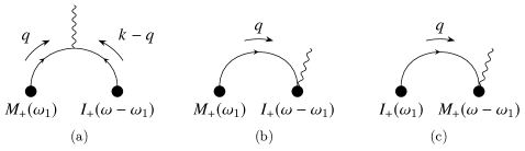
Figure 4: The Feynman diagrams needed for the computation of the tail contribution to $T_{+}^{\mu\nu}$. For simplicity we denote $k^{0}=\omega$ and $q^{0}=\omega_{1}$.

Appendix B Near-zone (local-in-time) GW fluxes

From the in-in computation, we will generally find the following form of the ‘dissipative’ part of the in-in effective action,

$$R_{\pm}=\sum_{\mathscr{M}}\mathscr{M}_{-}^{L}\mathscr{F}_{+}^{L}(\mathscr{M_{+}})\,,$$ (B.1)

where $\mathscr{M}_{-}^{L}$ is a generic multipole, $\mathscr{F}_{+}^{L}(\mathscr{M_{+}})$ is a function of the $\mathscr{M_{+}}$ multipoles, both contracted over $L$ indices. From here we obtain the energy and angular momentum losses from the near-zone dynamics (omitting the sum over particles for simplicity)

$$\dot{M} ={\boldsymbol{v}}\cdot\bigg{[}\frac{\partial\mathscr{M}_{-}^{L}}{\partial{\boldsymbol{x}}_{-}}\mathscr{F}_{+}^{L}(\mathscr{M_{+}})-\frac{{\mathrm{d}}}{{\mathrm{d}}t}\Bigg{(}\frac{\partial\mathscr{M}_{-}^{L}}{\partial{\boldsymbol{v}}_{-}}\mathscr{F}_{+}^{L}(\mathscr{M_{+}})\Bigg{)}\bigg{]}\bigg{|}_{\textrm{PL}}\,,$$ (B.2)

$$\dot{L}_{k} =\varepsilon_{kij}{\boldsymbol{x}}_{i}\bigg{[}\frac{\partial\mathscr{M}_{-}^{L}}{\partial{\boldsymbol{x}}^{j}_{-}}\mathscr{F}_{+}^{L}(\mathscr{M_{+}})-\frac{{\mathrm{d}}}{{\mathrm{d}}t}\Bigg{(}\frac{\partial\mathscr{M}_{-}^{L}}{\partial{\boldsymbol{v}}^{j}_{-}}\mathscr{F}_{+}^{L}(\mathscr{M_{+}})\Bigg{)}\bigg{]}\bigg{|}_{\textrm{PL}}\,.$$ (B.3)

Starting with (B.2), and upon time averaging over an orbit, we have Maia:2017gxn

$$\langle\dot{M}\rangle=\left\langle\bigg{[}{\boldsymbol{v}}\cdot\frac{\partial\mathscr{M}_{-}^{L}}{\partial{\boldsymbol{x}}_{-}}+\frac{{\mathrm{d}}{\boldsymbol{v}}}{{\mathrm{d}}t}\cdot\frac{\partial\mathscr{M}_{-}^{L}}{\partial{\boldsymbol{v}}_{-}}\bigg{]}\mathscr{F}_{+}^{L}(\mathscr{M_{+}})\right\rangle\bigg{|}_{\textrm{PL}}\,.$$ (B.4)

In order to evaluate the time derivatives, we use that

$$\frac{\partial\mathscr{M}_{-}^{L}}{\partial{\boldsymbol{x}}^{\ell}_{-}}\bigg{|}_{\textrm{PL}} =\bigg{(}\frac{\partial{\boldsymbol{x}}_{1}^{k}}{\partial x^{\ell}_{-}}\frac{\partial}{\partial{\boldsymbol{x}}_{1}^{k}}+\frac{\partial{\boldsymbol{x}}_{2}^{k}}{\partial{\boldsymbol{x}}^{\ell}_{-}}\frac{\partial}{\partial{\boldsymbol{x}}_{2}^{k}}\bigg{)}\Big{(}\mathscr{M}_{1}^{L}-\mathscr{M}_{2}^{L}\Big{)}\bigg{|}_{\textrm{PL}}$$

$$=\bigg{(}\frac{\delta^{k}{}_{\ell}}{2}\frac{\partial\mathscr{M}_{1}^{L}}{\partial{\boldsymbol{x}}_{1}^{k}}-\frac{(-\delta^{k}{}_{\ell})}{2}\frac{\partial\mathscr{M}_{2}^{L}}{\partial{\boldsymbol{x}}_{2}^{k}}\bigg{)}\bigg{|}_{\textrm{PL}}=\frac{\partial\mathscr{M}^{L}}{\partial{\boldsymbol{x}}^{\ell}}\,,$$ (B.5)

and similarly for the derivative with respect to the velocity. Hence, since the multipole moments do not depend explicitly on time (for a binary in isolation), we have

$$\frac{{\mathrm{d}}}{{\mathrm{d}}t}\mathscr{M}^{L}({\boldsymbol{x}}(t),{\boldsymbol{v}}(t))={\boldsymbol{v}}\cdot\frac{\partial\mathscr{M}^{L}}{\partial{\boldsymbol{x}}}+\frac{{\mathrm{d}}{\boldsymbol{v}}}{{\mathrm{d}}t}\cdot\frac{\partial\mathscr{M}^{L}}{\partial{\boldsymbol{v}}}\,,$$ (B.6)

such that

$$\langle\dot{M}\rangle=\left\langle\bigg{[}{\boldsymbol{v}}\cdot\frac{\partial\mathscr{M}^{L}}{\partial{\boldsymbol{x}}}+\frac{{\mathrm{d}}{\boldsymbol{v}}}{{\mathrm{d}}t}\cdot\frac{\partial\mathscr{M}^{L}}{\partial{\boldsymbol{v}}}\bigg{]}\mathscr{F}^{L}(\mathscr{M})\right\rangle=\left\langle\frac{{\mathrm{d}}\mathscr{M}^{L}}{{\mathrm{d}}t}\mathscr{F}^{L}(\mathscr{M})\right\rangle\,.$$ (B.7)

The computation of the angular-momentum flux is a bit trickier. Let us restrict the manipulations here local-in-time effects. We use the expression in (B.3) and, upon time-averaging, we get

$$\langle\dot{{\boldsymbol{L}}}_{k}\rangle=\varepsilon_{kij}\bigg{\langle}\bigg{[}{\boldsymbol{x}}_{i}\frac{\partial\mathscr{M}_{-}^{L}}{\partial{\boldsymbol{x}}^{j}_{-}}+{\boldsymbol{v}}_{i}\frac{\partial\mathscr{M}_{-}^{L}}{\partial{\boldsymbol{v}}^{j}_{-}}\bigg{]}\mathscr{F}_{+}^{L}(\mathscr{M_{+}})\bigg{\rangle}\bigg{|}_{\textrm{PL}}\,.$$ (B.8)

In what follows we particularize for our case at hand, namely $\mathscr{M}_{-}^{L}=\{L_{-}^{ij},I_{-}^{ij}\}$. Without loss of generality, the angular momentum and quadrupole may be decomposed as

$$L_{-}^{ij} =2f_{1}\big{(}{\boldsymbol{x}}_{-}^{[i}{\boldsymbol{v}}_{+}^{j]}+{\boldsymbol{x}}_{+}^{[i}{\boldsymbol{v}}_{-}^{j]}\big{)}$$ (B.9)

$$I_{-}^{ij} =\left(f_{2}\,{\boldsymbol{x}}_{-}^{(i}{\boldsymbol{x}}_{+}^{j)}+f_{3}\,{\boldsymbol{x}}_{-}^{(i}{\boldsymbol{v}}_{+}^{j)}+f_{4}\,{\boldsymbol{v}}_{-}^{(i}{\boldsymbol{x}}_{+}^{j)}+f_{5}\,{\boldsymbol{v}}_{-}^{(i}{\boldsymbol{v}}_{+}^{j)}\right)-{\rm traces}\,,$$ (B.10)

where the $f_{n}$’s, $n=1\cdots 5$, are only functions of the $+$ variables (with other contributions annihilated by the PL). For instance, at leading order we have

$$I_{-}^{ij}=\sum_{a}m_{a}\bigg{(}2{\boldsymbol{x}}_{a,-}^{(i}{\boldsymbol{x}}_{a,+}^{j)}-\frac{2}{3}\delta^{ij}{\boldsymbol{x}}_{a,-}\cdot{\boldsymbol{x}}_{a,+}\bigg{)}\,.$$ (B.11)

From the general form in the above expressions we find

$${\boldsymbol{x}}_{i}\frac{\partial L_{-}^{ab}}{\partial{\boldsymbol{x}}^{j}_{-}}+{\boldsymbol{v}}_{i}\frac{\partial L_{-}^{ab}}{\partial{\boldsymbol{v}}^{j}_{-}}\bigg{|}_{\textrm{PL}} =f_{1}\big{(}{\boldsymbol{x}}_{i}{\boldsymbol{v}}^{b}\delta_{j}{}^{a}+{\boldsymbol{x}}^{a}{\boldsymbol{v}}_{i}\delta_{j}{}^{b}-(a\leftrightarrow b)\big{)}=L_{i}{}^{b}\delta_{j}{}^{a}-L_{i}{}^{a}\delta_{j}{}^{b}\,$$ (B.12)

$${\boldsymbol{x}}_{i}\frac{\partial I_{-}^{ab}}{\partial{\boldsymbol{x}}^{j}_{-}}+{\boldsymbol{v}}_{i}\frac{\partial I_{-}^{ab}}{\partial{\boldsymbol{v}}^{j}_{-}}\bigg{|}_{\textrm{PL}} =2{\boldsymbol{x}}_{i}\big{(}f_{2}\,\delta_{j}{}^{(a}{\boldsymbol{x}}^{b)}+f_{3}\,\delta_{j}{}^{(a}{\boldsymbol{v}}^{b)}\big{)}+2{\boldsymbol{v}}_{i}\big{(}f_{4}\,\delta_{j}{}^{(a}{\boldsymbol{x}}^{b)}+f_{5}\,\delta_{j}{}^{(a}{\boldsymbol{v}}^{b)}\big{)}$$

$$=2I_{i}{}^{(a}\delta_{j}{}^{b)}+O\big{(}\delta_{i}{}^{(a}\delta_{j}{}^{b)}\big{)}\,,$$ (B.13)

where the last term represent the traces (that ultimately cancel out once contracted with antisymmetric terms). From here we arrive at the general structure for the flux of angular momentum

$$\langle\dot{{\boldsymbol{L}}}_{k}\rangle=\varepsilon_{kij}\left\langle I_{i\ell}\Big{(}\mathscr{F}_{\ell j}(\mathscr{M})+\mathscr{F}_{j\ell}(\mathscr{M})\Big{)}+L_{i\ell}\Big{(}\mathscr{F}_{j\ell}(\mathscr{M})-\mathscr{F}_{\ell j}(\mathscr{M})\Big{)}\right\rangle\,.$$ (B.14)

Appendix C Abraham-Lorentz conservative effects

The conservative relativistic scattering of two (nonspinning) charges in electrodynamics due to radiative effects was obtained in Bern:2023ccb , at fourth order in the coupling (see ancillary file in Bern:2023ccb ). Since (classical) electromagnetism is inherently a linear theory, the existence of such conservative-like terms can only be associated with contributions at second-order in the (linear) Abraham-(Dirac)-Lorentz force. We reproduce here this effect, at leading order in the PN expansion, from the point of view of the EFT approach Goldberger:2009qd ; Galley:2010es .

At leading order in the multipole expansion, and ignoring the gravitational field, the long-distance effective action for the two-body system takes the form

$$S_{\rm eff}=-\frac{1}{4}\int{\mathrm{d}}^{4}xF_{\mu\nu}F^{\mu\nu}-\sqrt{4\pi\alpha}(Q_{1}+Q_{2})\int{\mathrm{d}}t\,A^{\mu}V_{\mu}+\sqrt{4\pi\alpha}\int{\mathrm{d}}t\,{\boldsymbol{d}}\cdot{\boldsymbol{E}}+\cdots\,,$$ (C.1)

$$\alpha\equiv e^{2}/4\pi\,,\qquad F_{\mu\nu}=2\partial_{[\mu}A_{\nu]}\,,\qquad E_{i}=-F_{0i}$$ (C.2)

$$\quad V^{\mu}=\delta^{\mu}_{0}\,,\qquad{\boldsymbol{d}}(t)=Q_{1}{\boldsymbol{x}}_{1}(t)+Q_{2}{\boldsymbol{x}}_{2}(t)\,,$$

in the center-of-mass frame. We have only kept the coupling to the dipole, ${\boldsymbol{d}}$, which is the relevant term at leading PN order. In what follows we denote as $q_{a}\equiv Q_{a}/m_{a}$ ($a=1,2$) the charge/mass ratio.

In-in computation

We follow the same steps as in the gravitational case, yielding

$$iS[{\boldsymbol{x}}_{\pm}]=i(4\pi\alpha)\int\frac{{\mathrm{d}}\omega}{2\pi}\int_{{\boldsymbol{k}}}\bigg{[}k_{i}k_{j}d^{i}_{-}(-\omega)d_{+}^{j}(\omega)-\omega^{2}d^{i}_{-}(-\omega)d_{+}^{i}(\omega)\bigg{]}\frac{1}{(\omega+i0^{+})^{2}-{\boldsymbol{k}}^{2}}\,,$$ (C.3)

which reduces to

$$S[{\boldsymbol{x}}_{\pm}] =\frac{2\alpha}{3}\int\frac{{\mathrm{d}}\omega}{2\pi}(i\omega^{3})d^{i}_{-}(-\omega)d_{+}^{i}(\omega)=\frac{2\alpha}{3}\int{\mathrm{d}}t\,{\boldsymbol{d}}_{-}(t)\cdot{\boldsymbol{d}}^{(3)}_{+}(t)\,.$$ (C.4)

From the in-in action we get the radiation-reaction (Abraham-Lorentz) acceleration for each particle

$${\boldsymbol{a}}_{a\rm(RR)}=\frac{2\alpha}{3m_{a}}\frac{\partial{\boldsymbol{d}}_{-}(t)}{\partial{\boldsymbol{x}}_{a,-}(t)}\cdot{\boldsymbol{d}}^{(3)}_{+}(t)\bigg{|}_{\textrm{PL}}=\frac{2\alpha}{3}q_{a}{\boldsymbol{d}}^{(3)}(t)=\frac{2\alpha}{3}q_{a}\big{(}m_{1}q_{1}\dddot{{\boldsymbol{x}}}_{1}+m_{2}q_{2}\dddot{{\boldsymbol{x}}}_{2}\big{)}\,.$$ (C.5)

In order to obtain the leading order contribution, we replace the acceleration on the right-hand side of (C.5) by the Coulomb force, yielding the relative acceleration

$${\boldsymbol{a}}_{\rm(RR)} \equiv{\boldsymbol{a}}_{1\rm(RR)}-{\boldsymbol{a}}_{2\rm(RR)}=\frac{2}{3}\alpha^{2}M\nu\,q_{1}q_{2}(q_{1}-q_{2})^{2}\frac{{\mathrm{d}}}{{\mathrm{d}}t}\left(\frac{{\boldsymbol{r}}(t)}{r^{3}(t)}\right)\,.$$ (C.6a)

Since it is a total derivative, the contribution from this acceleration to the total impulse is clearly zero, regardless of the trajectory. That means that the only correction comes from the radiation-reaction deflected trajectory (or ‘iteration’ Kalin:2020mvi ) ${\boldsymbol{r}}(t)={\boldsymbol{b}}+{\boldsymbol{v}}_{\infty}t+\delta^{\rm(RR)}{\boldsymbol{r}}(t)$, which solves the equation

$$\frac{{\mathrm{d}}^{2}}{{\mathrm{d}}t^{2}}\delta^{(\textrm{RR})}{\boldsymbol{r}}(t)={\boldsymbol{a}}^{(\textrm{RR})}\,,$$ (C.7)

into the Coulomb force, yielding

$$\Delta^{(\textrm{RR})}{\boldsymbol{p}}_{1} =\frac{\alpha^{3}M^{4}}{b^{3}}\frac{q_{1}^{2}q_{2}^{2}(q_{1}-q_{2})^{2}\nu}{3v_{\infty}^{2}}\bigg{[}-4\frac{{\boldsymbol{b}}}{b}-\pi\frac{{\boldsymbol{v}}_{\infty}}{v_{\infty}}\bigg{]}\,,$$ (C.8a)

$$\Delta^{(\textrm{RR})}{\boldsymbol{p}}_{2} =m_{2}\int{\mathrm{d}}t{\boldsymbol{a}}^{C,(\textrm{RR},1)}_{2}(t)=\frac{\alpha^{3}M^{4}}{b^{3}}\frac{q_{1}^{2}q_{2}^{2}(q_{1}-q_{2})^{2}\nu}{3v_{\infty}^{2}}\bigg{[}4\frac{{\boldsymbol{b}}}{b}+\pi\frac{{\boldsymbol{v}}_{\infty}}{v_{\infty}}\bigg{]}\,,$$ (C.8b)

where, as in the main text, $({\boldsymbol{b}},{\boldsymbol{v}}_{\infty})$ are the impact parameter and relative velocity at infinity, respectively. This agrees with the nonrelativistic expansion of the result in Kalin:2022hph .

The acceleration at second order in the radiation-reaction (RR²) can be obtained by plugging back the radiation-reaction acceleration onto the right-hand side of the force,

$${\boldsymbol{a}}_{a\rm(RR^{2})} =\frac{4}{9}\alpha^{2}q_{a}\big{(}m_{1}q_{1}^{2}+m_{2}q_{2}^{2}\big{)}\frac{{\mathrm{d}}}{{\mathrm{d}}t}\bigg{[}m_{1}q_{1}\dddot{{\boldsymbol{x}}}_{1}+m_{2}q_{2}\dddot{{\boldsymbol{x}}}_{2}\bigg{]}\,$$ (C.9)

$$=\frac{4}{9}\alpha^{3}M^{2}\nu q_{a}\big{(}m_{1}q_{1}^{2}+m_{2}q_{2}^{2}\big{)}q_{1}q_{2}(q_{1}-q_{2})\frac{{\mathrm{d}}^{2}}{{\mathrm{d}}t^{2}}\frac{{\boldsymbol{r}}(t)}{r^{3}(t)}\,,$$

where in the last equality we inputed the Coulomb acceleration. Upon evaluating the time derivatives, we find

$${\boldsymbol{a}}_{a\rm(RR^{2})} =\frac{4}{9}\alpha^{3}M^{2}\nu q_{a}\big{(}m_{1}q_{1}^{2}+m_{2}q_{2}^{2}\big{)}q_{1}q_{2}(q_{1}-q_{2})$$ (C.10)

$$\times\bigg{[}\bigg{(}15\frac{{\boldsymbol{v}}\cdot{\boldsymbol{r}}}{r^{7}}-3\frac{v^{2}}{r^{5}}\bigg{)}{\boldsymbol{r}}-6\frac{({\boldsymbol{r}}\cdot{\boldsymbol{v}})}{r^{5}}{\boldsymbol{v}}-2\alpha mq_{1}q_{2}\frac{{\boldsymbol{r}}}{r^{6}}\bigg{]}\,.$$

such that

$${\boldsymbol{a}}_{\rm(RR^{2})} =\frac{4}{9}\alpha^{3}M^{2}\nu\big{(}m_{1}q_{1}^{2}+m_{2}q_{2}^{2}\big{)}q_{1}q_{2}(q_{1}-q_{2})^{2}$$ (C.11)

$$\times\bigg{[}\bigg{(}15\frac{{\boldsymbol{v}}\cdot{\boldsymbol{r}}}{r^{7}}-3\frac{v^{2}}{r^{5}}\bigg{)}{\boldsymbol{r}}-6\frac{({\boldsymbol{r}}\cdot{\boldsymbol{v}})}{r^{5}}{\boldsymbol{v}}-2\alpha mq_{1}q_{2}\frac{{\boldsymbol{r}}}{r^{6}}\bigg{]}\,,$$

for the relative acceleration, where the $\alpha^{4}$ term arises from the inclusion, once again, of the Coulomb force. Because of the structure of the radiation-reaction-square force, it is straightforward to show that

$$\int{\mathrm{d}}t{\boldsymbol{a}}_{a}^{(\textrm{RR}^{2})}\sim\bigg{[}\frac{{\mathrm{d}}}{{\mathrm{d}}t}\frac{{\boldsymbol{r}}(t)}{r^{3}(t)}\bigg{]}\bigg{|}^{\infty}_{-\infty}=0\,.$$ (C.12)

Since this integral vanishes, the nontrivial contribution the total impulse comes from evaluating the Coulomb acceleration on the trajectory deflected by the force in (C.11) to the desired order. We find

$$\Delta^{(\textrm{RR}^{2})}{\boldsymbol{p}}_{1}=-\pi\frac{\alpha^{4}M^{4}\nu^{2}}{b^{4}}\big{(}m_{1}q_{1}^{2}+m_{2}q_{2}^{2}\big{)}q_{1}^{2}q_{2}^{2}(q_{1}-q_{2})^{2}\frac{1}{3v_{\infty}}\frac{{\boldsymbol{b}}}{b}\,.$$ (C.13)

We discover $\Delta^{(\textrm{RR}^{2})}{\boldsymbol{p}}_{1}=-\Delta^{(\textrm{RR}^{2})}{\boldsymbol{p}}_{2}$, such that the contribution to the scattering angle becomes (using the same convention for a positive angle along the $-\hat{\boldsymbol{b}}$ direction)

$$\chi^{\rm tot}_{(\textrm{RR}^{2})}=\frac{|\Delta^{(\textrm{RR}^{2})}{\boldsymbol{p}}_{1}|}{M\nu v_{\infty}}=\pi\frac{\alpha^{4}M^{3}\nu}{3b^{4}v_{\infty}^{2}}\big{(}m_{1}q_{1}^{2}+m_{2}q_{2}^{2}\big{)}q_{1}^{2}q_{2}^{2}(q_{1}-q_{2})^{2}\,,$$ (C.14)

which, amusingly, also agrees at leading PN order with the conservative result in Bern:2023ccb . As we demonstrate next, this is expected due to the nature of the radiation-reaction-square force, and will be recovered as well from the in-out (Feynman) computation, as we demonstrate momentarily.

RR² force is conservative

Before proceeding, let us demonstrate that the radiation-reaction-square force in (C.10), to the order we are concerned about, is conservative. We already found the conservation of momentum. Let us look now at the loss of energy of each body, say particle 1,

$$\dot{E}_{1}\equiv m_{1}{\boldsymbol{v}}_{1}\cdot{\boldsymbol{a}}_{1(\textrm{RR}^{2})}=Am_{1}q_{1}\dot{{\boldsymbol{x}}}_{1}\cdot\frac{{\mathrm{d}}}{{\mathrm{d}}t}\bigg{[}m_{1}q_{1}\dddot{{\boldsymbol{x}}}_{1}+m_{2}q_{2}\dddot{{\boldsymbol{x}}}_{2}\bigg{]}\,,$$ (C.15)

where, in order to simplify notation, we introduced $A\equiv(4/9)\alpha^{2}\big{(}m_{1}q_{1}^{2}+m_{2}q_{2}^{2}\big{)}$. After performing the following manipulations

$$\dot{{\boldsymbol{x}}}_{1}\cdot\frac{{\mathrm{d}}}{{\mathrm{d}}t}\dddot{{\boldsymbol{x}}}_{1} =-\ddot{{\boldsymbol{x}}}_{1}\cdot\dddot{{\boldsymbol{x}}}_{1}+\frac{{\mathrm{d}}}{{\mathrm{d}}t}(\cdots)=-\frac{1}{2}\frac{{\mathrm{d}}}{{\mathrm{d}}t}\Big{(}\ddot{{\boldsymbol{x}}}_{1}^{2}+\cdots\Big{)}\,,$$ (C.16)

$$\dot{{\boldsymbol{x}}}_{1}\cdot\frac{{\mathrm{d}}}{{\mathrm{d}}t}\dddot{{\boldsymbol{x}}}_{2} =-\ddot{{\boldsymbol{x}}}_{1}\cdot\dddot{{\boldsymbol{x}}}_{2}+\frac{{\mathrm{d}}}{{\mathrm{d}}t}(\cdots)\,.$$ (C.17)

we find, up to total time derivatives,

$$\dot{E}_{1}=-Am_{1}m_{2}q_{1}q_{2}\,\ddot{{\boldsymbol{x}}}_{1}\cdot\dddot{{\boldsymbol{x}}}_{2}+\frac{{\mathrm{d}}}{{\mathrm{d}}t}(\cdots)\,.$$ (C.18)

and similarly,

$$\dot{E}_{2}=-Am_{2}m_{1}q_{1}q_{2}\ddot{{\boldsymbol{x}}}_{2}\cdot\dddot{{\boldsymbol{x}}}_{1}+\frac{{\mathrm{d}}}{{\mathrm{d}}t}(\cdots)\,.$$ (C.19)

so that

$$\dot{E}_{1}+\dot{E}_{2} =-Am_{2}q_{2}m_{1}q_{1}\Big{(}\ddot{{\boldsymbol{x}}}_{1}\cdot\dddot{{\boldsymbol{x}}}_{2}+\ddot{{\boldsymbol{x}}}_{2}\cdot\dddot{{\boldsymbol{x}}}_{1}\Big{)}+\frac{{\mathrm{d}}}{{\mathrm{d}}t}(\cdots)$$

$$=-Am_{2}q_{2}m_{1}q_{1}\frac{{\mathrm{d}}}{{\mathrm{d}}t}\Big{(}\ddot{{\boldsymbol{x}}}_{1}\cdot\ddot{{\boldsymbol{x}}}_{2}+\cdots\Big{)}=\frac{{\mathrm{d}}}{{\mathrm{d}}t}(\cdots)\,,$$ (C.20)

becomes a total derivative, which can then be moved to the left-hand side to define a new conserved quantity. Similar steps can be perform for the angular momentum. In that case we have

$$\dot{\boldsymbol{L}}^{i}_{1} =m_{1}\epsilon^{ijk}{\boldsymbol{x}}_{1}^{j}{\boldsymbol{a}}^{k}_{1(\rm RR^{2})}=Am_{1}q_{1}\epsilon^{ijk}{\boldsymbol{x}}_{1}^{j}\frac{{\mathrm{d}}}{{\mathrm{d}}t}\bigg{[}m_{1}q_{1}\dddot{{\boldsymbol{x}}}^{k}_{1}+m_{2}q_{2}\dddot{{\boldsymbol{x}}}^{k}_{2}\bigg{]}\,,$$ (C.21)

and using the identities,

$${\boldsymbol{x}}_{1}^{j}\frac{{\mathrm{d}}}{{\mathrm{d}}t}\dddot{{\boldsymbol{x}}}^{k}_{1} =-\dot{{\boldsymbol{x}}}_{1}^{j}\dddot{{\boldsymbol{x}}}^{k}_{1}+\frac{{\mathrm{d}}}{{\mathrm{d}}t}(\cdots)=\ddot{{\boldsymbol{x}}}_{1}^{j}\ddot{{\boldsymbol{x}}}^{k}_{1}+\frac{{\mathrm{d}}}{{\mathrm{d}}t}(\cdots)\,.$$ (C.22)

$${\boldsymbol{x}}_{1}^{j}\frac{{\mathrm{d}}}{{\mathrm{d}}t}\dddot{{\boldsymbol{x}}}^{k}_{2} =-\dot{{\boldsymbol{x}}}_{1}^{j}\dddot{x}^{k}_{2}+\frac{{\mathrm{d}}}{{\mathrm{d}}t}(\cdots)=\ddot{{\boldsymbol{x}}}_{1}^{j}\ddot{{\boldsymbol{x}}}^{k}_{2}+\frac{{\mathrm{d}}}{{\mathrm{d}}t}(\cdots)\,,$$ (C.23)

the only nontrivial contribution becomes

$$\dot{\boldsymbol{L}}^{i}_{1}=Am_{1}q_{1}m_{2}q_{2}\epsilon^{ijk}\ddot{{\boldsymbol{x}}}_{1}^{j}\ddot{{\boldsymbol{x}}}^{k}_{2}+\frac{{\mathrm{d}}}{{\mathrm{d}}t}(\cdots)\,.$$ (C.24)

and likewise for particle 2,

$$\dot{\boldsymbol{L}}^{i}_{2}=Am_{2}q_{2}m_{1}q_{1}\epsilon^{ijk}\ddot{{\boldsymbol{x}}}_{2}^{j}\ddot{{\boldsymbol{x}}}^{k}_{1}+\frac{{\mathrm{d}}}{{\mathrm{d}}t}(\cdots)\,,$$ (C.25)

such that, for the total loss of angular momentum we find,

$$\dot{\boldsymbol{L}}^{i}_{1}+\dot{\boldsymbol{L}}_{2}^{i}=Am_{2}m_{1}q_{2}q_{1}\epsilon^{ijk}\Big{(}\ddot{{\boldsymbol{x}}}_{1}^{j}\ddot{{\boldsymbol{x}}}^{k}_{2}+\ddot{{\boldsymbol{x}}}_{2}^{j}\ddot{{\boldsymbol{x}}}^{k}_{1}\Big{)}+\frac{{\mathrm{d}}}{{\mathrm{d}}t}(\cdots)=\frac{{\mathrm{d}}}{{\mathrm{d}}t}(\cdots)\,,$$ (C.26)

which, once again, becomes a total derivative.

In-out computation

We show now how to derive the conservative-like contribution to the scattering angle using the in-out approach. The effective action is obtained by integrating out the electromagnetic field. Following similar steps as before, we find

$$S^{\rm cons}_{\textrm{(RR)}} =-\frac{1}{3}(4\pi\alpha)\int\frac{{\mathrm{d}}\omega}{2\pi}\omega^{2}d^{i}(-\omega)d^{i}(\omega)\int_{{\boldsymbol{k}}}\frac{1}{(\omega+i0^{+})^{2}-{\boldsymbol{k}}^{2}}$$ (C.27)

$$=\frac{1}{3}\alpha\int\frac{{\mathrm{d}}\omega}{2\pi}(i\omega^{3})\textrm{Sign}(\omega)d^{i}(-\omega)d^{i}(\omega)=-i\frac{\alpha}{3\pi}\int{\mathrm{d}}t_{1}{\mathrm{d}}t_{2}\frac{\mathscr{P}}{t_{1}-t_{2}}{\boldsymbol{d}}(t_{1})\cdot{\boldsymbol{d}}^{(3)}(t_{2})\,,$$

The overall factor of $1/2$ difference with respect to the in-in result in (C.4) is due to the symmetry of the diagram, and in the last step we used (5.1). The reader will immediately notice that, provided the time derivatives of the dipole term are real functions of time (as expected from Coulomb-like interactions) the real part of the above in-out effective action vanishes, which is consistent with the fact that there is no conservative contribution at leading order in the radiation-reaction force. (The imaginary part, on the other hand, directly leads to the well-known dipole emission formula: $P\sim{\boldsymbol{d}}^{(2)}\cdot{\boldsymbol{d}}^{(2)}$, as expected from the optical theorem Porto:2016pyg .) We can, nonetheless, obtain an acceleration using the generalized Euler-Lagrangian equations Galley:2014wla ,

$${\boldsymbol{F}}_{a}=\frac{\partial\mathcal{L}}{\partial{\boldsymbol{x}}_{a}(t)}-\frac{{\mathrm{d}}}{{\mathrm{d}}t}\frac{\partial\mathcal{L}}{\partial\dot{{\boldsymbol{x}}}_{a}(t)}+\frac{{\mathrm{d}}^{2}}{{\mathrm{d}}t^{2}}\frac{\partial\mathcal{L}}{\partial\ddot{{\boldsymbol{x}}}_{a}(t)}-\frac{{\mathrm{d}}^{3}}{{\mathrm{d}}t^{3}}\frac{\partial\mathcal{L}}{\partial\dddot{{\boldsymbol{x}}}_{a}(t)}+\cdots\,,$$ (C.28)

and we get

$${\boldsymbol{F}}^{\rm cons}_{\rm(RR)a} =-\frac{i\alpha}{3\pi}Q_{a}\int{\mathrm{d}}t_{1}{\mathrm{d}}t_{1}\bigg{[}\delta(t-t_{1})\frac{\mathscr{P}}{t_{1}-t_{2}}{\boldsymbol{d}}^{(3)}(t_{2})-{\boldsymbol{d}}(t_{1})\frac{{\mathrm{d}}^{3}}{{\mathrm{d}}t^{3}}\bigg{(}\frac{\mathscr{P}}{t_{1}-t_{2}}\delta(t-t_{2})\bigg{)}\bigg{]}\,$$ (C.29)

$$=-\frac{2i\alpha}{3\pi}Q_{a}\int{\mathrm{d}}t^{\prime}\frac{\mathscr{P}}{t-t^{\prime}}{\boldsymbol{d}}^{(3)}(t^{\prime})=-\frac{2i\alpha}{3\pi}m_{a}q_{a}\int{\mathrm{d}}t^{\prime}\frac{\mathscr{P}}{t-t^{\prime}}\big{(}m_{1}q_{1}\dddot{{\boldsymbol{x}}}_{1}(t^{\prime})+m_{2}q_{2}\dddot{{\boldsymbol{x}}}_{2}(t^{\prime})\big{)}\,.$$

The fact that the leading radiation-reaction force is imaginary is a consequence of the fact that radiative effects dissipative energy at leading order, and therefore, from the decomposition of the retarded Green’s function into a Feynman term plus a cut Kalin:2022hph , only the latter contributes. However, that is no longer the case at second order, as we demonstrate in what follows.

To obtain the radiation-reaction-square effects, we replace the second derivatives in (C.29) with the very same acceleration, yielding

$${\boldsymbol{a}}^{\rm cons}_{{\rm(RR^{2})}a} =-\frac{4\alpha^{2}}{9\pi^{2}}q_{a}\int{\mathrm{d}}t^{\prime}\frac{\mathscr{P}}{t-t^{\prime}}\bigg{[}m_{1}q_{1}^{2}\frac{{\mathrm{d}}}{{\mathrm{d}}t^{\prime}}\int{\mathrm{d}}t^{\prime\prime}\frac{\mathscr{P}}{t^{\prime}-t^{\prime\prime}}\bigg{(}m_{1}q_{1}\dddot{{\boldsymbol{x}}}_{1}(t^{\prime\prime})+m_{2}q_{2}\dddot{{\boldsymbol{x}}}_{2}(t^{\prime\prime})\bigg{)}$$

$$\hskip 85.35826pt+m_{2}q_{2}^{2}\frac{{\mathrm{d}}}{{\mathrm{d}}t^{\prime}}\int{\mathrm{d}}t^{\prime\prime}\frac{\mathscr{P}}{t^{\prime}-t^{\prime\prime}}\bigg{(}m_{1}q_{1}\dddot{{\boldsymbol{x}}}_{1}(t^{\prime\prime})+m_{2}q_{2}\dddot{{\boldsymbol{x}}}_{2}(t^{\prime\prime})\bigg{)}\bigg{]}$$

$$=-\frac{4\alpha^{2}}{9\pi^{2}}q_{a}(m_{1}q_{1}^{2}+m_{2}q_{2}^{2})\int{\mathrm{d}}t^{\prime}\frac{\mathscr{P}}{t-t^{\prime}}\int{\mathrm{d}}t^{\prime\prime}\frac{\mathscr{P}}{t^{\prime}-t^{\prime\prime}}\bigg{(}m_{1}q_{1}{\boldsymbol{x}}^{(4)}_{1}(t^{\prime\prime})+m_{2}q_{2}{\boldsymbol{x}}^{(4)}_{2}(t^{\prime\prime})\bigg{)}\,.$$ (C.30)

We invoke again the Poincaré-Bertrand theorem Davies:1990fe ; Davies:1996gee (see (5.4)) and exchange the order of integration, yielding

$${\boldsymbol{a}}^{\rm cons}_{{\rm(RR^{2})}a} =-\frac{4\alpha^{2}}{9\pi^{2}}q_{a}(m_{1}q_{1}^{2}+m_{2}q_{2}^{2})\int{\mathrm{d}}t^{\prime\prime}\big{(}m_{1}q_{1}{\boldsymbol{x}}^{(4)}_{1}(t^{\prime\prime})+m_{2}q_{2}{\boldsymbol{x}}^{(4)}_{2}(t^{\prime\prime})\big{)}\int{\mathrm{d}}t^{\prime}\frac{\mathscr{P}}{(t-t^{\prime})(t^{\prime}-t^{\prime\prime})}$$

$$+\frac{4\alpha^{2}}{9}q_{a}(m_{1}q_{1}^{2}+m_{2}q_{2}^{2})\big{(}m_{1}q_{1}{\boldsymbol{x}}^{(4)}_{1}(t)+m_{2}q_{2}{\boldsymbol{x}}^{(4)}_{2}(t)\big{)}$$

$$=\frac{4\alpha^{2}}{9}q_{a}(m_{1}q_{1}^{2}+m_{2}q_{2}^{2})\big{(}m_{1}q_{1}{\boldsymbol{x}}^{(4)}_{1}(t)+m_{2}q_{2}{\boldsymbol{x}}^{(4)}_{2}(t)\big{)}\,,\par$$ (C.31)

where in the last equality we used the fact that Davies:1990fe ; Davies:1996gee

$$\int{\mathrm{d}}t\frac{\mathscr{P}}{(t-t^{\prime})(t^{\prime}-t^{\prime\prime})}=0\,.$$ (C.32)

We are thus left with the exact same acceleration in (C.9) from the in-in approach, which implies that the contributions from the reactive terms all vanish at this order. Following the same steps as before, we get the same value for the scattering angle, consistently with the relativistic result in Bern:2023ccb .

Radial action

It is instructive to derive the contribution from radiation-reaction-square effects also directly at the level of the (radial) action. This can be done replacing the second derivative in (C.27) with the acceleration in (C.29), together with (C.32), yielding

$$S_{(\textrm{RR}^{2})}^{\rm cons} =-\frac{2\alpha^{2}}{9\pi^{2}}\big{(}m_{1}q_{1}^{2}+m_{2}q_{2}^{2}\big{)}\int{\mathrm{d}}t_{1}{\boldsymbol{d}}(t_{1})\cdot\int{\mathrm{d}}t_{2}\frac{\mathscr{P}}{t_{1}-t_{2}}\int{\mathrm{d}}t_{3}\frac{\mathscr{P}}{t_{2}-t_{3}}{\boldsymbol{d}}_{\rm(RR)}^{(4)}(t_{3})$$

$$=\frac{2\alpha^{2}}{9}\big{(}m_{1}q_{1}^{2}+m_{2}q_{2}^{2}\big{)}\int{\mathrm{d}}t\,{\boldsymbol{d}}(t)\cdot{\boldsymbol{d}}_{\rm(RR)}^{(4)}(t)\,,$$ (C.33)

where

$${\boldsymbol{d}}_{\rm(RR)}^{(4)}(t)=\alpha M^{2}\nu q_{1}q_{2}(q_{1}-q_{2})\frac{{\mathrm{d}}^{2}}{{\mathrm{d}}t^{2}}\left(\frac{{\boldsymbol{r}}(t)}{r^{3}(t)}\right)\,,$$ (C.34)

such that

$$S_{(\textrm{RR}^{2})}^{\rm cons}=\frac{2\alpha^{3}}{9}M^{2}\nu\big{(}m_{1}q_{1}^{2}+m_{2}q_{2}^{2}\big{)}q_{1}q_{2}(q_{1}-q_{2})\int{\mathrm{d}}t\,{\boldsymbol{d}}(t)\cdot\frac{{\mathrm{d}}^{2}}{{\mathrm{d}}t^{2}}\left(\frac{{\boldsymbol{r}}(t)}{r^{3}(t)}\right)\,.$$ (C.35)

From here we can relate the conservative action, evaluated on the (leading) Coulomb trajectory, to the scattering angle via (see e.g. Bini:2021gat )

$$\chi^{\rm cons}_{\rm(RR^{2})}=-\frac{\partial}{\partial J}S_{(\textrm{RR}^{2})}^{\rm cons}\,,$$ (C.36)

with $J=M\nu v_{\infty}b$ the total angular momentum. Upon inputing the solution for the trajectory, we arrive at

$$S_{(\textrm{RR}^{2})}^{\rm cons}=\pi\frac{\alpha^{4}M^{4}\nu^{2}}{9b^{3}v_{\infty}}\big{(}m_{1}q_{1}^{2}+m_{2}q_{2}^{2}\big{)}q_{1}^{2}q_{2}^{2}(q_{1}-q_{2})^{2}\,,$$ (C.37)

from which we find

$$\chi^{\rm cons}_{\rm(RR^{2})}=\pi\frac{\alpha^{4}M^{3}\nu}{3b^{4}v_{\infty}^{2}}\big{(}m_{1}q_{1}^{2}+m_{2}q_{2}^{2}\big{)}q_{1}^{2}q_{2}^{2}(q_{1}-q_{2})^{2}\,,$$ (C.38)

in agreement with (C.14), which implies as before that $\chi^{\rm tot}_{\rm(RR^{2})}=\chi^{\rm cons}_{\rm(RR^{2})}$ at this order.

References

• (1) KAGRA, VIRGO, LIGO Scientific collaboration, GWTC-3: Compact Binary Coalescences Observed by LIGO and Virgo during the Second Part of the Third Observing Run, Phys. Rev. X 13 (2023) 041039 [2111.03606].
• (2) LISA collaboration, Laser Interferometer Space Antenna, 1702.00786.
• (3) M. Punturo et al., The Einstein Telescope: A third-generation gravitational wave observatory, Class. Quant. Grav. 27 (2010) 194002.
• (4) D. Reitze et al., Cosmic Explorer: The U.S. Contribution to Gravitational-Wave Astronomy beyond LIGO, Bull. Am. Astron. Soc. 51 (2019) 035 [1907.04833].
• (5) A. Buonanno and B. S. Sathyaprakash, Sources of Gravitational Waves: Theory and Observations. 10, 2014. 1410.7832.
• (6) R. A. Porto, The Music of the Spheres: The Dawn of Gravitational Wave Science, 1703.06440.
• (7) R. Alves Batista et al., EuCAPT White Paper: Opportunities and Challenges for Theoretical Astroparticle Physics in the Next Decade, 2110.10074.
• (8) S. Bernitt et al., Fundamental Physics in the Gravitational-Wave Era, Nucl. Phys. News 32 (2022) 16.
• (9) L. Blanchet, Gravitational Radiation from Post-Newtonian Sources and Inspiralling Compact Binaries, Living Rev. Rel. 17 (2014) 2 [1310.1528].
• (10) G. Schäfer and P. Jaranowski, Hamiltonian formulation of general relativity and post-Newtonian dynamics of compact binaries, Living Rev. Rel. 21 (2018) 7 [1805.07240].
• (11) L. Barack and A. Pound, Self-force and radiation reaction in general relativity, Rept. Prog. Phys. 82 (2019) 016904 [1805.10385].
• (12) W. D. Goldberger and I. Z. Rothstein, An Effective field theory of gravity for extended objects, Phys. Rev. D 73 (2006) 104029 [hep-th/0409156].
• (13) R. A. Porto, Post-Newtonian corrections to the motion of spinning bodies in NRGR, Phys. Rev. D 73 (2006) 104031 [gr-qc/0511061].
• (14) W. D. Goldberger and A. Ross, Gravitational radiative corrections from effective field theory, Phys. Rev. D 81 (2010) 124015 [0912.4254].
• (15) C. R. Galley and M. Tiglio, Radiation reaction and gravitational waves in the effective field theory approach, Phys. Rev. D 79 (2009) 124027 [0903.1122].
• (16) C. R. Galley, D. Tsang and L. C. Stein, The principle of stationary nonconservative action for classical mechanics and field theories, 1412.3082.
• (17) R. A. Porto, The effective field theorist’s approach to gravitational dynamics, Phys. Rept. 633 (2016) 1 [1601.04914].
• (18) G. Kälin and R. A. Porto, From Boundary Data to Bound States, JHEP 01 (2020) 072 [1910.03008].
• (19) G. Kälin and R. A. Porto, From boundary data to bound states. Part II. Scattering angle to dynamical invariants (with twist), JHEP 02 (2020) 120 [1911.09130].
• (20) G. Kälin and R. A. Porto, Post-Minkowskian Effective Field Theory for Conservative Binary Dynamics, JHEP 11 (2020) 106 [2006.01184].
• (21) G. Mogull, J. Plefka and J. Steinhoff, Classical black hole scattering from a worldline quantum field theory, JHEP 02 (2021) 048 [2010.02865].
• (22) S. Mougiakakos, M. M. Riva and F. Vernizzi, Gravitational Bremsstrahlung in the post-Minkowskian effective field theory, Phys. Rev. D 104 (2021) 024041 [2102.08339].
• (23) C. Dlapa, G. Kälin, Z. Liu and R. A. Porto, Dynamics of binary systems to fourth Post-Minkowskian order from the effective field theory approach, Phys. Lett. B 831 (2022) 137203 [2106.08276].
• (24) C. Dlapa, G. Kälin, Z. Liu and R. A. Porto, Conservative Dynamics of Binary Systems at Fourth Post-Minkowskian Order in the Large-Eccentricity Expansion, Phys. Rev. Lett. 128 (2022) 161104 [2112.11296].
• (25) G. Cho, G. Kälin and R. A. Porto, From boundary data to bound states. Part III. Radiative effects, JHEP 04 (2022) 154 [2112.03976].
• (26) G. Cho, R. A. Porto and Z. Yang, Gravitational radiation from inspiralling compact objects: Spin effects to the fourth post-Newtonian order, Phys. Rev. D 106 (2022) L101501 [2201.05138].
• (27) G. Kälin, J. Neef and R. A. Porto, Radiation-reaction in the Effective Field Theory approach to Post-Minkowskian dynamics, JHEP 01 (2023) 140 [2207.00580].
• (28) C. Dlapa, G. Kälin, Z. Liu, J. Neef and R. A. Porto, Radiation Reaction and Gravitational Waves at Fourth Post-Minkowskian Order, Phys. Rev. Lett. 130 (2023) 101401 [2210.05541].
• (29) G. U. Jakobsen, G. Mogull, J. Plefka and B. Sauer, All things retarded: radiation-reaction in worldline quantum field theory, JHEP 10 (2022) 128 [2207.00569].
• (30) W. D. Goldberger, Effective field theories of gravity and compact binary dynamics: A Snowmass 2021 whitepaper, in Snowmass 2021, 6, 2022, 2206.14249.
• (31) C. Dlapa, G. Kälin, Z. Liu and R. A. Porto, Bootstrapping the relativistic two-body problem, JHEP 08 (2023) 109 [2304.01275].
• (32) C. Dlapa, G. Kälin, Z. Liu and R. A. Porto, Local in Time Conservative Binary Dynamics at Fourth Post-Minkowskian Order, Phys. Rev. Lett. 132 (2024) 221401 [2403.04853].
• (33) L. Amalberti, Z. Yang and R. A. Porto, Gravitational radiation from inspiralling compact binaries to N3LO in the effective field theory approach, Phys. Rev. D 110 (2024) 044046 [2406.03457].
• (34) D. Neill and I. Z. Rothstein, Classical Space-Times from the S Matrix, Nucl. Phys. B 877 (2013) 177 [1304.7263].
• (35) N. E. J. Bjerrum-Bohr, P. H. Damgaard, G. Festuccia, L. Planté and P. Vanhove, General Relativity from Scattering Amplitudes, Phys. Rev. Lett. 121 (2018) 171601 [1806.04920].
• (36) C. Cheung, I. Z. Rothstein and M. P. Solon, From Scattering Amplitudes to Classical Potentials in the Post-Minkowskian Expansion, Phys. Rev. Lett. 121 (2018) 251101 [1808.02489].
• (37) Z. Bern, C. Cheung, R. Roiban, C.-H. Shen, M. P. Solon and M. Zeng, Black Hole Binary Dynamics from the Double Copy and Effective Theory, JHEP 10 (2019) 206 [1908.01493].
• (38) A. Brandhuber, G. Chen, G. Travaglini and C. Wen, Classical gravitational scattering from a gauge-invariant double copy, JHEP 10 (2021) 118 [2108.04216].
• (39) Z. Bern, J. Parra-Martinez, R. Roiban, M. S. Ruf, C.-H. Shen, M. P. Solon et al., Scattering Amplitudes, the Tail Effect, and Conservative Binary Dynamics at O(G4), Phys. Rev. Lett. 128 (2022) 161103 [2112.10750].
• (40) P. Di Vecchia, C. Heissenberg, R. Russo and G. Veneziano, The gravitational eikonal: From particle, string and brane collisions to black-hole encounters, Phys. Rept. 1083 (2024) 1 [2306.16488].
• (41) M. Campanelli, C. O. Lousto, P. Marronetti and Y. Zlochower, Accurate evolutions of orbiting black-hole binaries without excision, Phys. Rev. Lett. 96 (2006) 111101 [gr-qc/0511048].
• (42) F. Pretorius, Evolution of binary black hole spacetimes, Phys. Rev. Lett. 95 (2005) 121101 [gr-qc/0507014].
• (43) L. Blanchet and T. Damour, Hereditary effects in gravitational radiation, Phys. Rev. D 46 (1992) 4304.
• (44) L. Blanchet, Quadrupole-quadrupole gravitational waves, Class. Quant. Grav. 15 (1998) 89 [gr-qc/9710037].
• (45) L. Blanchet, G. Faye, Q. Henry, F. Larrouturou and D. Trestini, Gravitational-Wave Phasing of Quasicircular Compact Binary Systems to the Fourth-and-a-Half Post-Newtonian Order, Phys. Rev. Lett. 131 (2023) 121402 [2304.11185].
• (46) T. Damour, P. Jaranowski and G. Schäfer, Nonlocal-in-time action for the fourth post-Newtonian conservative dynamics of two-body systems, Phys. Rev. D 89 (2014) 064058 [1401.4548].
• (47) C. R. Galley, A. K. Leibovich, R. A. Porto and A. Ross, Tail effect in gravitational radiation reaction: Time nonlocality and renormalization group evolution, Phys. Rev. D 93 (2016) 124010 [1511.07379].
• (48) L. Bernard, L. Blanchet, A. Bohé, G. Faye and S. Marsat, Fokker action of nonspinning compact binaries at the fourth post-Newtonian approximation, Phys. Rev. D 93 (2016) 084037 [1512.02876].
• (49) T. Marchand, L. Bernard, L. Blanchet and G. Faye, Ambiguity-Free Completion of the Equations of Motion of Compact Binary Systems at the Fourth Post-Newtonian Order, Phys. Rev. D 97 (2018) 044023 [1707.09289].
• (50) S. Foffa and R. Sturani, Conservative dynamics of binary systems to fourth Post-Newtonian order in the EFT approach I: Regularized Lagrangian, Phys. Rev. D 100 (2019) 024047 [1903.05113].
• (51) S. Foffa, R. A. Porto, I. Rothstein and R. Sturani, Conservative dynamics of binary systems to fourth Post-Newtonian order in the EFT approach II: Renormalized Lagrangian, Phys. Rev. D 100 (2019) 024048 [1903.05118].
• (52) R. A. Porto and I. Z. Rothstein, Apparent ambiguities in the post-Newtonian expansion for binary systems, Phys. Rev. D 96 (2017) 024062 [1703.06433].
• (53) T. Damour, P. Jaranowski and G. Schäfer, Conservative dynamics of two-body systems at the fourth post-Newtonian approximation of general relativity, Phys. Rev. D 93 (2016) 084014 [1601.01283].
• (54) R. A. Porto, Lamb shift and the gravitational binding energy for binary black holes, Phys. Rev. D 96 (2017) 024063 [1703.06434].
• (55) S. Foffa and R. Sturani, Hereditary terms at next-to-leading order in two-body gravitational dynamics, Phys. Rev. D 101 (2020) 064033 [1907.02869].
• (56) Q. Henry, G. Faye and L. Blanchet, The current-type quadrupole moment and gravitational-wave mode ($\ell$, m) = (2, 1) of compact binary systems at the third post-Newtonian order, Class. Quant. Grav. 38 (2021) 185004 [2105.10876].
• (57) L. Amalberti, F. Larrouturou and Z. Yang, Multipole expansion at the level of the action in d-dimensions, Phys. Rev. D 109 (2024) 104027 [2312.02868].
• (58) G. L. Almeida, S. Foffa and R. Sturani, Tail contributions to gravitational conservative dynamics, Phys. Rev. D 104 (2021) 124075 [2110.14146].
• (59) J. Blümlein, A. Maier, P. Marquard and G. Schäfer, The fifth-order post-Newtonian Hamiltonian dynamics of two-body systems from an effective field theory approach, Nucl. Phys. B 983 (2022) 115900 [2110.13822].
• (60) D. Bini, T. Damour and A. Geralico, Radiative contributions to gravitational scattering, Phys. Rev. D 104 (2021) 084031 [2107.08896].
• (61) M. Driesse, G. U. Jakobsen, G. Mogull, J. Plefka, B. Sauer and J. Usovitsch, Conservative Black Hole Scattering at Fifth Post-Minkowskian and First Self-Force Order, 2403.07781.
• (62) J. Blümlein, A. Maier, P. Marquard and G. Schäfer, The fifth-order post-Newtonian Hamiltonian dynamics of two-body systems from an effective field theory approach: potential contributions, Nucl. Phys. B 965 (2021) 115352 [2010.13672].
• (63) G. L. Almeida, S. Foffa and R. Sturani, Gravitational radiation contributions to the two-body scattering angle, Phys. Rev. D 107 (2023) 024020 [2209.11594].
• (64) G. L. Almeida, A. Müller, S. Foffa and R. Sturani, Conservative binary dynamics from gravitational tail emission processes, Phys. Rev. D 108 (2023) 124010 [2307.05327].
• (65) L. V. Keldysh, Diagram technique for nonequilibrium processes, Zh. Eksp. Teor. Fiz. 47 (1964) 1515.
• (66) E. Calzetta and B. L. Hu, Nonequilibrium Quantum Fields: Closed Time Path Effective Action, Wigner Function and Boltzmann Equation, Phys. Rev. D 37 (1988) 2878.
• (67) C. R. Galley, A. K. Leibovich and I. Z. Rothstein, Finite size corrections to the radiation reaction force in classical electrodynamics, Phys. Rev. Lett. 105 (2010) 094802 [1005.2617].
• (68) C. R. Galley and A. K. Leibovich, Radiation reaction at 3.5 post-Newtonian order in effective field theory, Phys. Rev. D 86 (2012) 044029 [1205.3842].
• (69) W. D. Goldberger, A. Ross and I. Z. Rothstein, Black hole mass dynamics and renormalization group evolution, Phys. Rev. D 89 (2014) 124033 [1211.6095].
• (70) C. R. Galley and R. A. Porto, Gravitational self-force in the ultra-relativistic limit: the ”large-$N$” expansion, JHEP 11 (2013) 096 [1302.4486].
• (71) N. T. Maia, C. R. Galley, A. K. Leibovich and R. A. Porto, Radiation reaction for spinning bodies in effective field theory II: Spin-spin effects, Phys. Rev. D 96 (2017) 084065 [1705.07938].
• (72) N. T. Maia, C. R. Galley, A. K. Leibovich and R. A. Porto, Radiation reaction for spinning bodies in effective field theory I: Spin-orbit effects, Phys. Rev. D 96 (2017) 084064 [1705.07934].
• (73) W. D. Goldberger, J. Li and I. Z. Rothstein, Non-conservative effects on spinning black holes from world-line effective field theory, JHEP 06 (2021) 053 [2012.14869].
• (74) W. D. Goldberger and I. Z. Rothstein, Horizon radiation reaction forces, JHEP 10 (2020) 026 [2007.00731].
• (75) A. K. Leibovich, B. A. Pardo and Z. Yang, Radiation reaction for nonspinning bodies at 4.5PN in the effective field theory approach, Phys. Rev. D 108 (2023) 024017 [2302.11016].
• (76) K. G. Arun, L. Blanchet, B. R. Iyer and S. Sinha, Third post-Newtonian angular momentum flux and the secular evolution of orbital elements for inspiralling compact binaries in quasi-elliptical orbits, Phys. Rev. D 80 (2009) 124018 [0908.3854].
• (77) Q. Henry and F. Larrouturou, Conservative tail and failed-tail effects at the fifth post-Newtonian order, Phys. Rev. D 108 (2023) 084048 [2307.05860].
• (78) Z. Bern, E. Herrmann, R. Roiban, M. S. Ruf, A. V. Smirnov, V. A. Smirnov et al., Conservative binary dynamics at order $O(\alpha^{5})$ in electrodynamics, 2305.08981.
• (79) W. L. Burke and K. S. Thorne, Gravitational Radiation Damping, in Relativity Conference in the Midwest, pp. 209–228, 1970, DOI.
• (80) W. D. Goldberger and I. Z. Rothstein, Dissipative effects in the worldline approach to black hole dynamics, Phys. Rev. D 73 (2006) 104030 [hep-th/0511133].
• (81) B. S. DeWitt, Quantum Theory of Gravity. 2. The Manifestly Covariant Theory, Phys. Rev. 162 (1967) 1195.
• (82) G. ’t Hooft and M. J. G. Veltman, One loop divergencies in the theory of gravitation, Ann. Inst. H. Poincare Phys. Theor. A 20 (1974) 69.
• (83) L. F. Abbott, The Background Field Method Beyond One Loop, Nucl. Phys. B 185 (1981) 189.
• (84) M. Maggiore, Gravitational Waves. Vol. 1: Theory and Experiments. Oxford University Press, 2007, 10.1093/acprof:oso/9780198570745.001.0001.
• (85) D. Bini and A. Geralico, Higher-order tail contributions to the energy and angular momentum fluxes in a two-body scattering process, Phys. Rev. D 104 (2021) 104020 [2108.05445].
• (86) K. T. R. Davies, G. D. White and R. W. Davies, Dispersion relations for causal Green’s functions: Derivations using the Poincare-Bertrand theorem and its generalizations, J. Math. Phys. 31 (1990) 1356.
• (87) K. t. r. Davies, M. l. Glasser, V. Protopopescu and F. Tabakin, THE MATHEMATICS OF PRINCIPAL VALUE INTEGRALS AND APPLICATIONS TO NUCLEAR PHYSICS, TRANSPORT THEORY, AND CONDENSED MATTER PHYSICS, Math. Models Methods Appl. Sci. 06 (1996) 833.
• (88) D. Bini and T. Damour, Fourth Post-Minkowskian Local-in-Time Conservative Dynamics of Binary Systems, 2406.04878.
• (89) D. Bini, T. Damour and A. Geralico, Radiated momentum and radiation reaction in gravitational two-body scattering including time-asymmetric effects, Phys. Rev. D 107 (2023) 024012 [2210.07165].
• (90) A. V. Manohar, A. K. Ridgway and C.-H. Shen, Radiated Angular Momentum and Dissipative Effects in Classical Scattering, Phys. Rev. Lett. 129 (2022) 121601 [2203.04283].
• (91) P. Di Vecchia, C. Heissenberg and R. Russo, Angular momentum of zero-frequency gravitons, JHEP 08 (2022) 172 [2203.11915].
• (92) M. M. Riva, F. Vernizzi and L. K. Wong, Angular momentum balance in gravitational two-body scattering: Flux, memory, and supertranslation invariance, Phys. Rev. D 108 (2023) 104052 [2302.09065].
• (93) C. Heissenberg and R. Russo, Revisiting gravitational angular momentum and mass dipole losses in the eikonal framework, 6, 2024, 2406.03937.
• (94) D. Bini, T. Damour, S. De Angelis, A. Geralico, A. Herderschee, R. Roiban et al., Gravitational waveforms: A tale of two formalisms, Phys. Rev. D 109 (2024) 125008 [2402.06604].
• (95) A. Georgoudis, C. Heissenberg and R. Russo, Post-Newtonian multipoles from the next-to-leading post-Minkowskian gravitational waveform, Phys. Rev. D 109 (2024) 106020 [2402.06361].
• (96) D. Bini, T. Damour and A. Geralico, Gravitational Bremsstrahlung Waveform at the fourth Post-Minkowskian order and the second Post-Newtonian level, 2407.02076.
• (97) Alan Müller and Riccardo Sturani. Private Communication.