Asymptotic Preserving Linearly Implicit Additive IMEX-RK Finite Volume Schemes for Low Mach Number Isentropic Euler Equations

Abstract

We consider the compressible Euler equations of gas dynamics with isentropic equation of state. In the low Mach number regime i.e. when the fluid velocity is very very small in comparison to the sound speed in the medium, the solution of the compressible system converges to the solution of its incompressible counter part. Standard numerical schemes fail to respect this transition property and hence are plagued with inaccuracies as well as instabilities. In this paper we introduce an extra flux term to the momentum flux. This extra term is brought to fore by looking at the incompressibility constraints of the asymptotic limit system. This extra flux term enables us to get a suitable flux splitting, so that an additive IMEX-RK scheme could be applied. Using an elliptic reformulation the scheme boils down to just solving a linear elliptic problem for the density and then explicit updates for the momentum. The IMEX schemes developed are shown to be formally asymptotically consistent with the low Mach number limit of the Euler equations. A second order space time fully discrete scheme is obtained in the finite volume framework using a combination of Rusanov flux for the explicit part and simple central differences for the implicit part. Numerical results are reported which elucidate the theoretical assertions regarding the scheme and its robustness.

[2010] Primary 35L45, 35L60, 35L65, 35L67; Secondary 65M06, 65M08

1 Introduction

The compressible Euler equations of gas dynamics serve as a staple for fluid dynamics models. Therefore, they attracts a lot of attention for development of numerical schemes. They have been as relevant today as they ever were in the history, owing to their ability to express multiple flow regimes and, inability of numerical schemes to capture all at once. The compressible Euler equations are typically studied, from the perspective of numerical schemes for two distinct and complementary fluid regimes, namely

• compressible regime: where the reference sound speed of the medium is of the same order as of the speed of the fluid under consideration; and

• weakly compressible or incompressible (low Mach) regime: where the sound speed is of orders of magnitude more than that of the velocity of the fluid under consideration.

In this paper it is the low Mach number regime for which we endeavour to design and analyse a class of numerical schemes. Typically the Euler equations once subjected to appropriate non-dimensionalisation via appropriate scaling parameters reveals a singular perturbation parameter many a times denoted by $\varepsilon$ which is a scaled Mach number [2, 9]. Strictly speaking the incompressible limit or regime is only achieved at the limit of $\varepsilon\to 0$. But, in practice $\varepsilon$ values in the vicinity of $\mathcal{O}(10^{-1})$ or $\mathcal{O}(10^{-2})$ signify the weakly compressible regime and values smaller than that are considered for flows which are more or less incompressible.

Standard explicit schemes find it a hard task to maintain stability requirements when summoned for weakly incompressible flows, let alone incompressible flow. This is because of dire CFL stability restriction which enforces that the time steps are $\mathcal{O}(\varepsilon)$. Resulting to a practically almost non evolving scheme in the incompressible regime. Having said this solving the stability issue doesn’t still render a good numerical scheme. The numerical schemes also suffer from inaccuracies in the incompressible regime. The inaccuracy of the numerical solution, and inability of the numerical method to respect the transitional behaviour of the equations are mainly due to the loss of information in the passage from continuous to discrete level. We refer the reader to [10, 12, 17] and the references therein for a detailed account of the above-mentioned anomalies.

The convergence of solutions of the compressible Euler equations to those of the incompressible Euler equations in the limit of zero Mach number, and the associated challenges in numerical approximation is an active area of research. The asymptotic preserving (AP) framework provides a robust framework to address these issues. An AP scheme has two main characteristic features, exactly aiming to remedy the above noted challenges associated with the numerical approximation of plasma flows, which are:

• its stability requirements are independent of the multiscale or a singular parameter;

• in the limit of the singular parameter, the numerical scheme transforms itself to a scheme for the limit system.

The notion of AP schemes was initially introduced by Jin [14] for kinetic transport equations; see also [8, 15] for a comprehensive review of this subject. The procedure takes into account the transitional behaviour of the governing equations of the problem, and its stability requirements are independent of the singular perturbation parameter. Hence, an AP scheme for the compressible Euler equations automatically transforms to an incompressible solver when the Mach number goes to zero. As discussed in [8], semi-implicit time-stepping techniques provide a systematic approach to derive AP schemes; see, e.g. [4, 7, 9, 18, 20], for some semi-implicit AP schemes for the Euler or shallow water equations.

The literature for AP schemes for Euler equations in the low Mach regime is quite abundant; see [2, 6, 11] and the references therein for a detailed exposure. To the best of out knowledge the pursuit to find an additive implicit explicit (IMEX) scheme [19] which is linearly implicit is still going on. Typically the pressure term in the momentum is considered to be implicit in an additive IMEX scheme for the Euler equation. And this pressure term is non-linearly dependent on density. This lead to a semi-implicit scheme which is still non-linear needing for employment of a Newton solve. In [6] the authors have developed IMEX scheme which are linearly implicit, but are not additively split. This is primarily the problem that we have focused on in this paper.

The rest of this paper is organised as follows. In Section 2, we present the governing equations i.e. the Euler equations of gas dynamics with which are appropriately non-dimensionalised leading to a singular perturbation problem with a singular parameter $\varepsilon$, the scaled Mach number. Further, we present a formal derivation of the incompressible limit system. This analysis helps us later to choose an appropriate term which is added to the momentum flux [9, 2].In Section 3, we introduce an additional flux term which enables us to realise an appropriate flux splitting to propose a first order time-semi discrete numerical scheme. The first order scheme is analysed and shown to be asymptotically consistent with the incompressible limit system.Section 4 is devoted to higher extension of the first order scheme, which is obtained by the application of additive IMEX-RK scheme [3, 19]. The space discretisation technique is presented in Section 5, which is based on the finite volume framework. In Section 6 some numerical case studies are carried out to test and display the high-order accuracy, AP property and the performance of the IMEX-RK schemes schemes. Finally, the paper is closed in Section 7 with some conclusions and future plans for further extension of the schemes to more general equation of states.

2 Euler Equations Scaled With Low Mach Regime References

Consider the scaled non-dimensionalised Euler equations.

(1) $$\partial_{t}\rho+\nabla\cdot\mbox{\boldmath$q$}=0$$

(2) $$\partial_{t}\mbox{\boldmath$q$}+\nabla\cdot\left(\frac{\mbox{\boldmath$q$}\otimes\mbox{\boldmath$q$}}{\rho}\right)+\frac{\mathrm{\nabla}p}{\varepsilon^{2}}=0,$$

where $\rho(t,\mbox{\boldmath$x$})\in\mathbb{R}$ is the density, $\mbox{\boldmath$q$}(t,\mbox{\boldmath$x$})=\rho\mbox{\boldmath$u$}\in\mathbb{R}^{d}$, $d=1,2,3$ is the momentum and $p(t,\mbox{\boldmath$x$})=p(\rho)\in\mathbb{R}$ is the pressure. To close the system we assume either the system is isentropic or isothermal in nature, via a density pressure power law:

(3) $$p(\rho)=\rho^{\gamma},\qquad\mbox{where}\ \gamma=1\ \mbox{for isothermal,}\ \mbox{and}\ \gamma>1\ \mbox{for isentropic gases}.$$

In the above system $\varepsilon$ is a singular perturbation parameter which is the scaled Mach number i.e.

(4) $$\varepsilon=\mbox{Ma}:=\frac{u_{\mbox{ref}}}{p_{\mbox{ref}}\ \rho_{\mbox{ref}}}.$$

To formally derive the singular limits of the scaled isentropic Euler equation system (1)-(2) we assume that all the dependent variables i.e. $\rho,\mbox{\boldmath$q$},p$ assume the following multiscale ansatz:

(5) $$f(t,x)=f_{(0)}(t,x)+\varepsilon f_{(1)}(t,x)+\varepsilon^{2}f_{(2)}(t,x)$$

2.1 Zero Mach Number Limit $\varepsilon\to 0$

In order to obtain the zero Mach number limit of the Euler equations (1)-(2) in the limit of $\varepsilon\to 0$ we plugin the ansatz (5) in the above scaled euler equation system for all the dependent variables and equate like powers of $\varepsilon$ . The $\mathcal{O}(\varepsilon^{-2})$ terms in the momentum equations (2) give:

(6) $$\nabla p_{(0)}=0,$$

and then using the equation of state (EOS) (3) we get:

(7) $$\nabla\rho_{(0)}=0,$$

or the leading order density $\rho_{(0)}$ is spatially constant. Similarly, considering $\mathcal{O}(\varepsilon^{-1})$ terms in the momentum balance equations (1) we get that the first-order density $\rho_{(1)}$ is also spatially constant. Therefore the density can be considered to have the following expansion:

(8) $$\rho(t,x)=\rho_{(0)}(t)+\varepsilon^{2}\rho_{(2)}(t,x).$$

Now considering the $\mathcal{O}(\varepsilon^{0})$ terms in the mass conservation equation (1) and integrating over a spatial domain $\Omega$, leads us to:

(9) $$\frac{d}{dt}\int_{\Omega}\rho_{(0)}dx=\int_{\Omega}\nabla\cdot(\rho_{(0)}u_{(0)})dx=\int_{\partial\Omega}(\rho_{(0)}u_{(0)})\cdot\nu\ d\sigma.$$

Assuming periodic or no-flux boundary condition would lead to the right hand side integral of the above equation to vanish, yielding the independence of $\rho_{(0)}$ from the temporal variable $t$. Using the fact that $\rho_{(0)}$ is constant in (9) would give the incompressibility i.e. the divergence free condition for the velocity $u_{(0)}$ as:

(10) $$\nabla\cdot u_{(0)}=0.$$

Finally, considering the $\mathcal{O}(\varepsilon^{0})$ terms of the momentum equation (2), coupling it with the divergence condition (10) we get the zero Mach number limit system as:

(11) $$\partial_{t}u_{(0)}+\nabla\cdot\left(u_{(0)}\otimes u_{(0)}\right)+\nabla p_{(2)} =0,$$

(12) $$\nabla\cdot u_{(0)} =0.$$

Here the unknowns are the zeroth order velocity $u_{(0)}$ and the second order pressure $p_{(2)}$. To be precise, $p_{(2)}$ is scaled by the constant $\rho_{(0)}$ in the above system. The above set of equations are nothing but the standard incompressible Euler system for the unknowns $u_{(0)}$ and $p_{(2)}$.

Remark 2.1.

The incompressible limit system (11)-(12) is of mixed hyperbolic-elliptic in nature, and it doesn’t support acoustic waves. The second order pressure $P_{(2)}$ survives as the incompressible pressure and it plays the role of a Lagrange multiplier to enforce the divergence-free constraint (12). By taking the divergence of (11), we get the following reformulated zero Mach number incompressible limit system:

(13) $$\partial_{t}u_{(0)}+\nabla\cdot\left(u_{(0)}\otimes u_{(0)}\right)+\nabla p_{(2)}=0,$$

(14) $$\Delta p_{(2)}=-\nabla^{2}:\left(u_{(0)}\otimes u_{(0)}\right).$$

For smooth solutions the zero Mach number limit system (11)-(12) and the reformulated zero Mach number limit system (13)-(14) are equivalent.

Remark 2.2.

As $\rho_{(2)}$ features no where in the limit system one can ignore it completely to conclude that for the zero Mach number scaling doesn’t admit any perturbation in density.

3 Time Discretisation

In this section we present the design and analysis of first-order time semi-discrete Runge-Kutta (RK) schemes for the Euler equation (1)-(2). This first-order scheme is formally analysed to illustrate its AP property.

Based on the analysis of the Euler equations (1)-(2) presented in the previous section we introduce the following definition of a well-prepared data.

Definition 3.1.

A tuple $(\rho,\mbox{\boldmath$q$})$ of solutions to the compressible Euler equation system (1)-(2) is said to be well-prepared if the following decompositions hold:

(15) $$\rho =\rho_{(0)}+\varepsilon^{2}\rho_{(2)}$$

(16) $$u =\mbox{\boldmath$u$}_{(0)}+\varepsilon\mbox{\boldmath$u$}_{(1)},$$

where:

$$\nabla\rho_{(0)}=0\qquad\mbox{and}\qquad\nabla\cdot u_{(0)}=0.$$

3.1 Equilibrium Addition

The asymptotic analysis presented in the previous section shows that the obtaining the formal incompressibility condition hinges on a very fundamental constraint, which is

(17) $$\nabla\rho_{(0)}=0.$$

And this is true for the density of the incompressible system as well. As a consequence we want to somehow be able to preserve this state of density. As a resort we add and subtract the gradient of the density scaled by $1/\varepsilon^{2}$, to the momentum equation (2) to obtain the following:

(18) $$\partial_{t}\mbox{\boldmath$q$}+\nabla\cdot\left(\frac{\mbox{\boldmath$q$}\otimes\mbox{\boldmath$q$}}{\rho}\right)+\frac{\mathrm{\nabla}(p-\rho)}{\varepsilon^{2}}+\frac{\mathrm{\nabla}\rho}{\varepsilon^{2}}=0,$$

Note that the above equation is equivalent to the original momentum equation (2). Now, we propose a first order scheme for the Euler equations (1) and (18).

3.2 First Order Time Semi-discrete Scheme

To obtain a first-order accurate semi-implicit time discretisation the mass flux is treated implicitly and the momentum flux, which is now a combination of the constraint $\mathrm{\nabla}\rho=0$ is treated partly implicit and partly explicit.

Definition 3.2.

The first-order time semi-discrete scheme updates the solution $(\rho^{n},q^{n})$ at time $t^{n}$ to $(\rho^{n+1},q^{n+1})$ at time $t^{n+1}$ via the following semi-implicit updates:

(19) $$\frac{\rho^{n+1}-\rho^{n}}{\Delta t}+\nabla\cdot\mbox{\boldmath$q$}^{n+1}=0$$

(20) $$\frac{\mbox{\boldmath$q$}^{n+1}-\mbox{\boldmath$q$}^{n}}{\Delta t}+\nabla\cdot\left(\frac{\mbox{\boldmath$q$}^{n}\otimes\mbox{\boldmath$q$}^{n}}{\rho^{n}}\right)+\frac{\nabla(p^{n}-\rho^{n})}{\varepsilon^{2}}+\frac{\mathrm{\nabla}\rho^{n+1}}{\varepsilon^{2}}=0,$$

We follow the approach of [9] to obtain a reformulation of the above scheme. It is the reformulation instead which is implemented. To this end we rewrite the momentum update (20) as follows:

(21) $$\mbox{\boldmath$q$}^{n+1}=\hat{\mbox{\boldmath$q$}}^{n+1}-\Delta t\frac{\mathrm{\nabla}\rho^{n+1}}{\varepsilon^{2}},$$

where $\hat{\mbox{\boldmath$q$}}^{n+1}$ is the part that can be explicitly updated i.e.

(22) $$\hat{\mbox{\boldmath$q$}}^{n+1}:=\mbox{\boldmath$q$}^{n}-\Delta t\nabla\cdot\left(\frac{\mbox{\boldmath$q$}^{n}\otimes\mbox{\boldmath$q$}^{n}}{\rho^{n}}\right)-\Delta t\frac{\nabla(p^{n}-\rho^{n})}{\varepsilon^{2}}.$$

Now substituting for $\mbox{\boldmath$q$}^{n+1}$ from (21) in the mass update (19) we get the following elliptic problem for $\rho^{n+1}$:

$$\rho^{n+1}=\rho^{n}-\Delta t\nabla\cdot(\hat{\mbox{\boldmath$q$}}^{n+1}-\Delta t\frac{\mathrm{\nabla}\rho^{n+1}}{\varepsilon^{2}}).$$

Definition 3.3.

The first-order reformulated time semi-discrete scheme updates the solution $(\rho^{n},\mbox{\boldmath$q$}^{n})$ at time $t^{n}$ to $(\rho^{n+1},\mbox{\boldmath$q$}^{n+1})$ at time $t^{n+1}$ by first evaluating $\hat{\mbox{\boldmath$q$}}^{n+1}$ via (22) and then $\rho^{n+1}$ is obtained as a solution of the following linear elliptic problem:

(23) $$-\frac{\Delta t^{2}}{\varepsilon^{2}}\Delta\rho^{n+1}+\rho^{n+1}=\rho^{n}-\Delta t\nabla\cdot\hat{\mbox{\boldmath$q$}}^{n+1}.$$

and then $\mbox{\boldmath$q$}^{n+1}$ is obtained as an explicit update via:

(24) $$\mbox{\boldmath$q$}^{n+1}=\hat{\mbox{\boldmath$q$}}^{n+1}-\Delta t\frac{\nabla\rho^{n+1}}{\varepsilon^{2}},$$

where $\hat{\mbox{\boldmath$q$}}^{n+1}$ contains the terms which can be explicitly evaluated.

Remark 3.4.

Note that the reformulated first-order time semi-discrete scheme is computationally twice as efficient as the first-order semi-discrete scheme in Defintion 3.2. As there is only one elliptic problem, that to for the density variable $\rho^{n+1}$ that has to be solved in case of Defintion 3.3. Where as in the other case depending on the number of spatial dimension the inversion matrix will be larger and larger.

Proposition 3.5.

The first-order time semi-discrete scheme in Definition 3.2 and the reformulated first-order time semi-discrete scheme in Definition 3.3, are equivalent.

Remark 3.6.

As both the above presented schemes are equivalent it is the reformulated time semi discrete scheme in Definition 3.3 which is the one which is used for implementation owing to its computational efficiency.

Proposition 3.7.

Suppose that the data at time $t^{n}$ are well-prepared i.e. $(\rho^{n},\mbox{\boldmath$u$}^{n})$ admit the decomposition in Definition 3.1. Then if the solution $(\rho^{n+1},\mbox{\boldmath$u$}^{n+1})$ defined by the scheme in Definition 3.3 admits the multiscale decomposition (15)-(16), then it is well-prepared as well. Further, the semi-discrete scheme in Definition 3.3 reduces to a consistent discretisation of the low Mach incompressible limit system, in other words the scheme is asymptotically consistent.

Proof 3.8.

To start with note that $(\rho^{n+1},u^{n+1})$ are assumed to admit the following ansatz:

(25) $$\rho^{n+1} =\rho^{n+1}_{(0)}+\varepsilon^{2}\rho^{n+1}_{(2)}$$

$$\mbox{\boldmath$u$}^{n+1} =\mbox{\boldmath$u$}^{n+1}_{(0)}+\varepsilon\mbox{\boldmath$u$}^{n+1}_{(1)}$$

Plugging in the above in (20) and considering the $\mathcal{O}(\varepsilon^{-2})$ terms yield:

(26) $$\mathrm{\nabla}(p_{(0)}^{n}-\rho_{(0)}^{n})-\nabla\rho^{n+1}_{(0)}=0$$

as the data is assumed to be well-prepared at time $t^{n}$, we have $\mathrm{\nabla}(p_{(0)}-\rho_{(0)})=0$. Therefore, the above equation implies:

(27) $$\mathrm{\nabla}\rho^{n+1}_{(0)}=0$$

Now integrating the $\mathcal{O}(\varepsilon^{0})$ terms of the mass update (19) over a domain $\Omega$ and upon the imposition of appropriate boundary conditions gives us :

(28) $$\rho_{(0)}^{n+1}=\rho_{(0)}^{n}=\mbox{const}.$$

Again using the above in the mass update (19) would yield the divergence condition for the velocity i.e.

(29) $$\nabla\cdot\mbox{\boldmath$u$}^{n+1}=0.$$

Lastly, looking at the $\mathcal{O}(\varepsilon^{0})$ terms of the momentum update (20) gives:

(30) $$\frac{\mbox{\boldmath$u$}^{n+1}_{(0)}-\mbox{\boldmath$u$}^{n}_{(0)}}{\Delta t}+\nabla\cdot(\mbox{\boldmath$u$}_{(0)}\otimes\mbox{\boldmath$u$}_{(0)})++\frac{\mathrm{\nabla}(p_{(2)}^{n}-\rho_{(2)}^{n})}{\rho_{(0)}^{n}}+\frac{\nabla\rho^{n+1}_{(2)}}{\rho_{(0)}^{n}}=0,$$

which is a consistent discretisation of the limit equation (11) with $p_{(2)}^{n+1}$ identified as $p_{(2)}^{n}-\rho_{(2)}^{n}+\rho_{(2)}^{n+1}$.

4 Higher Order Extension of Time Discretisation

The time discretisation strategy introduced in the previous section splits the new momentum flux. All the non-linear flux terms are treated explicitly and implicitness is associated only with a linear flux. The splitting under consideration for the first order discretisation is additive in nature. Therefore it is well suited to extend the time discretisation using the addtive IMEX-RK strategy from [3, 19].

4.1 IMEX-RK Time Discretisation

IMEX-RK schemes provide a robust and efficient framework to design AP schemes for singular perturbation problems. In this work, we only consider a subclass of the IMEX-RK schemes, namely diagonally implicit or (DIRK) schemes. An $s$-stage IMEX-RK scheme is characterised by the two $s\times s$ lower triangular matrices $\tilde{A}=(\tilde{a}_{i,j})$, and $A=(a_{i,j})$, the coefficients $\tilde{c}=(\tilde{c}_{1},\tilde{c}_{2},\ldots,\tilde{c}_{s})$ and $c=(c_{1},c_{2},\ldots,c_{s})$, and the weights $\tilde{\omega}=(\tilde{\omega}_{1},\tilde{\omega}_{2},\ldots,\tilde{\omega}_{s})$ and $\omega=(\omega_{1},\omega_{2},\ldots,\omega_{s})$. Here, the entries of $\tilde{A}$ and $A$ satisfy the conditions $\tilde{a}_{i,j}=0$ for $j\geq i$, and $a_{i,j}=0$ for $j>i$. Let us consider the following stiff system of ODEs in an additive form:

(31) $$y^{\prime}=f(t,y)+\frac{1}{\varepsilon}g(t,y),$$

where $0<\varepsilon\ll 1$ is called the stiffness parameter. The functions $f$ and $g$ are known as, respectively, the non-stiff part and the stiff part of the system (31); see, e.g. [13], for a comprehensive treatment of such systems.

Let $y^{n}$ be a numerical solution of (31) at time $t^{n}$ and let $\Delta t$ denote a fixed timestep. An $s$-stage IMEX-RK scheme, cf., e.g. [3, 19], updates $y^{n}$ to $y^{n+1}$ through $s$ intermediate stages:

(32) $$Y_{i} =y^{n}+\Delta t\sum\limits_{j=1}^{i-1}\tilde{a}_{i,j}f(t^{n}+\tilde{c}_{j}\Delta t,Y_{j})+\Delta t\sum\limits_{j=1}^{s}a_{i,j}\frac{1}{\varepsilon}g(t^{n}+c_{j}\Delta t,Y_{j}),\ 1\leq i\leq s,$$

(33) $$y^{n+1} =y^{n}+\Delta t\sum\limits_{i=1}^{s}\tilde{\omega}_{i}f(t^{n}+\tilde{c}_{i}\Delta t,Y_{i})+\Delta t\sum\limits_{i=1}^{s}\omega_{i}\frac{1}{\varepsilon}g(t^{n}+c_{i}\Delta t,Y_{i}).$$

The above IMEX-RK scheme (32)-(33) can be symbolically represented by the double Butcher tableau:

$\tilde{c}^{T}$	$\tilde{A}$
	$\tilde{\omega}^{T}$

$c^{T}$	$A$
	$\omega^{T}$

Figure 1: Double Butcher tableau of an IMEX-RK scheme.

The coefficients $\tilde{c}_{i}$ and $c_{i}$ and the weights $\tilde{\omega}_{i}$ and $\omega_{i}$ are fixed by the order conditions; see [19] for details. In order to further simplify the analysis of the schemes presented in this paper, we restrict ourselves only to two types of DIRK schemes, namely the type-A and type-CK schemes which are defined below; see [16] for details.

Definition 4.1.

An IMEX-RK scheme is said to be of

• type-A, if the matrix $A$ is invertible;

• type-CK, if the matrix $A\in\mathbb{R}^{s\times s},\ s\geq 2$, can be written as

  $$A=\begin{pmatrix}0&0\\ \alpha&A_{s-1}\end{pmatrix},$$

  where $\alpha\in\mathbb{R}^{s-1}$ and $A_{s-1}\in\mathbb{R}^{s-1\times s-1}$ is invertible.

4.2 Higher Order Time Discretisation for the Euler Equations

Definition 4.2.

An $s$-stage IMEX-RK schemes for the Euler equations (1)-(2) updates the solution $(\rho^{n},\mbox{\boldmath$q$}^{n})$ at time $t^{n}$ to $(\rho^{n+1},\mbox{\boldmath$q$}^{n+1})$ at time $t^{n+1}$ via the following $s$ intermediate stages:

(34) $$\rho^{k} =\rho^{n}-\Delta t\sum_{\ell=1}^{k}a_{k,\ell}\nabla\cdot\mbox{\boldmath$q$}^{\ell}$$

(35) $$\mbox{\boldmath$q$}^{k} =\mbox{\boldmath$q$}^{n}-\Delta t\sum_{\ell=1}^{k-1}\tilde{a}_{k,\ell}\left(\nabla\cdot\left(\frac{\mbox{\boldmath$q$}^{\ell}\otimes\mbox{\boldmath$q$}^{\ell}}{\rho^{\ell}}\right)+\mathrm{\nabla}(p^{\ell}-\rho^{\ell})\right)-\Delta t\sum_{\ell=1}^{k}a_{k,\ell}\mathrm{\nabla}\rho^{\ell},$$

where $k=1,\ldots,s$. As we choose only stiffly accurate schemes the final update is the same as the update at the last ($s^{th}$) stage i.e. the numerical solution at time $t^{n+1}$ is given by:

(36) $$(\rho^{n+1},\mbox{\boldmath$q$}^{n+1})=(\rho^{s},\mbox{\boldmath$q$}^{s})$$

As was done for the first order time semi-discrete scheme here also we derive a reformulation based on [9], which is equivalent to the scheme presented above. To this end we write the mass (34) and momentum (35) updates as follows:

(37) $$\rho^{k} =\hat{\rho}^{n}-\Delta ta_{k,k}\nabla\cdot\mbox{\boldmath$q$}^{k}$$

(38) $$\mbox{\boldmath$q$}^{k} =\hat{\mbox{\boldmath$q$}}^{k}-\Delta ta_{k,k}\mathrm{\nabla}\rho^{k},$$

where $\hat{\rho}^{k}$ and $\hat{\mbox{\boldmath$q$}}^{k}$ are respectively the part of the mass and momentum updates which can be evaluated fully explicitly at the $k^{th}$ stage,i.e.

(39) $$\hat{\rho}^{k} :=\rho^{n}-\Delta t\sum_{\ell=1}^{k-1}a_{k,\ell}\nabla\cdot\mbox{\boldmath$q$}^{\ell}$$

(40) $$\hat{\mbox{\boldmath$q$}}^{k} :=\mbox{\boldmath$q$}^{n}-\Delta t\sum_{\ell=1}^{k-1}\tilde{a}_{k,\ell}\left(\nabla\cdot\left(\frac{\mbox{\boldmath$q$}^{\ell}\otimes\mbox{\boldmath$q$}^{\ell}}{\rho^{\ell}}\right)+\mathrm{\nabla}(p^{\ell}-\rho^{\ell})\right)-\Delta t\sum_{\ell=1}^{k-1}a_{k,\ell}\mathrm{\nabla}\rho^{\ell}$$

Now, having recast both the mass and momentum updates we use (38) to substitute for $\mbox{\boldmath$q$}^{k}$ in the recasted mass update (37) to get the following elliptic problem for $\rho^{k}$:

(41) $$-\frac{\Delta t^{2}a_{k,k}^{2}}{\varepsilon^{2}}\Delta\rho^{k}+\rho^{k}=\hat{\rho}^{k}-\Delta t\hat{\mbox{\boldmath$q$}}^{k}$$

Definition 4.3.

The $s$-stage reformulated IMEX-RK time semi-discrete scheme for the Euler equations (1)-(2) updates the solution $(\rho^{n},u^{n})$ via $s$ intermediate stages , where the $k^{th}$ stage is given by:

• The explicit part of mass and momentum $\hat{\rho}^{k}$ and $\hat{\mbox{\boldmath$q$}}^{k}$ are first updated via (39) and (40), respectively.

• Solve the elliptic problem (41) for $\rho^{k}$.

• Finally, update $\mbox{\boldmath$q$}^{k}$ using the $\rho^{k}$ obtained in the previous step via (38).

Proposition 4.4.

The high-order time semi-discrete scheme in Definition 4.2 and the reformulated high-order time semi-discrete scheme in Definition 4.3, are equivalent.

Remark 4.5.

As both the above presented schemes are equivalent it is the reformulated time semi discrete scheme in Definition 4.3 which is the one which is used for implementation owing to its computational efficiency.

Proposition 4.6.

Suppose that the data at time $t^{n}$ are well-prepared i.e. $(\rho^{n},\mbox{\boldmath$u$}^{n})$ admit the decomposition in Definition 3.1. Then if the solution $(\rho^{n+1},\mbox{\boldmath$u$}^{n+1})$ defined by the scheme in Definition 4.3 admits the multiscale decomposition (15)-(16), then it is well-prepared as well. Further, the semi-discrete scheme in Definition 4.3 reduces to a consistent discretisation of the low Mach incompressible limit system, in other words the higher order IMEX-RK scheme is asymptotically consistent.

5 Space-Time Fully Discrete Finite Volume IMEX-RK Schemes

In this section the reformulated high-order time discretisation will be coupled with an appropriate space discretisation strategy to obtain a fully discrete implementable numerical scheme. To this end, a second order fully discrete scheme in the finite volume framework is obtained by a combination of Rusanov flux for the explicit fluxes and a second order central differencing for implicit fluxes.

To make the presentation of the fully discrete scheme very compact let us introduced thethe vector $i=(i_{1},i_{2},i_{3})$ where each $i_{m}$ for $m=1,2,3$ represent $x_{m}$ the space direction. We further introduce the following finite difference and averaging operators: e.g. in the $x_{m}$-direction

(42) $$\delta_{x_{m}}w_{i}=w_{i+\frac{1}{2}e_{m}}-w_{i-\frac{1}{2}e_{m}},\quad\mu_{x_{m}}w_{i}=\frac{w_{i+\frac{1}{2}e_{m}}+w_{i-\frac{1}{2}e_{m}}}{2},$$

for any grid function $w_{i}$. We denote the explicit momentum flux by $F$ where each of its $m^{th}$component is given by

(43) $$F_{m}(U)=\frac{q_{m}}{\rho}q+(p-\rho)e_{m}$$

Definition 5.1.

The $k^{th}$ stage of the $s$-stage fully discrete IMEX scheme for the Euler equation system is defined as follows. The explicit variables are computed first as:

(44) $$\hat{\rho}^{k}_{i} =\rho^{n}_{i}-\sum_{l=1}^{k-1}a_{k,l}\sum_{m=1}^{3}\nu_{m}\delta_{x_{m}}\mathcal{G}_{m,i}^{l},$$

(45) $$\hat{q}^{k}_{i} =q^{n}_{i}-\sum_{l=1}^{k-1}\tilde{a}_{k,l}\sum_{m=1}^{3}\nu_{m}\delta_{x_{m}}\mathcal{F}_{m,i}^{l}+\sum_{l=1}^{k-1}a_{k,l}\sum_{m=1}^{3}\nu_{m}\delta_{x_{m}}\mu_{x_{m}}\rho_{i}^{l}e_{m}$$

Following, the above update $\rho^{k}_{i}$ is updated by solving the following elliptic problem:

(46) $$\sum_{m=1}^{3}\frac{\delta_{x_{m}}}{\Delta x_{m}}\left(\frac{\delta_{x_{m}}}{\Delta x_{m}}\rho^{k}_{i}\right)+\rho^{k}_{i}=\hat{\rho}_{i}^{k}-a_{k,k}\sum_{m=1}^{3}\nu_{m}\delta_{x_{m}}\hat{q}_{m,i}^{k},$$

Followed by the explicit evaluations,

(47) $$q^{k}_{m,i}=\hat{q}^{k}_{m,i}-\Delta ta_{i,i}\nu_{m}\delta_{x_{m}}\rho_{i}^{k},\quad m=1,2\mbox{ and }3$$

Here, the repeated index $m$ takes values in $\{1,2,3\}$, $\nu_{m}:=\frac{\Delta t}{\Delta x_{m}}$ denote the mesh ratios and the vector $(\mathcal{G}_{m})$ is an approximation of the mass flux $q$, $\mathcal{F}_{m}$ is an approximation of the $m^{th}$ element of the flux $F$ in (43) and the are defined as:

(48) $$\mathcal{G}^{l}_{m,i+\frac{1}{2}e_{m}} =\frac{1}{2}(q^{l}_{m,i+e_{m}}+q^{l}_{m,i})$$

$$\mathcal{F}^{l}_{m,i+\frac{1}{2}e_{m}} =\frac{1}{2}\left(F_{m}(U^{l,+}_{i+\frac{1}{2}e_{m}})+F_{m}(U^{l,-}_{i+\frac{1}{2}e_{m}})\right)-\frac{\alpha_{m,i+\frac{1}{2}e_{m}}}{2}\left(q_{m,i+\frac{1}{2}e_{m}}^{k,+}-q_{m,i+\frac{1}{2}e_{m}}^{k,-}\right)$$

Here, for any conservative variable $w$, we have denoted by $w^{\pm}_{i+\frac{1}{2}e_{m}}$, the interpolated states obtained using the piecewise linear reconstructions. The wave-speeds are computed as, e.g. in the $x_{1}$-direction

(49) $$\alpha_{1,i+\frac{1}{2}e_{1}}:=2\max\left(\left|\frac{q_{1,i+\frac{1}{2}e_{1}}^{k,-}}{\rho_{i+\frac{1}{2}e_{1}}^{k,-}}\right|,\left|\frac{q_{1,i+\frac{1}{2}e_{1}}^{k,+}}{\rho_{i+\frac{1}{2}e_{1}}^{k,+}}\right|\right).$$

The momentum flux $F$ is approximated by a Rusanov-type flux, and the the mass flux is approximated using simple central differences. Hence, the eigenvalues of the Jacobians of the part of the flux which is approximated by Rusanov-type flux can be obtained as $\lambda_{m,1}=0,\lambda_{m,2}=\lambda_{m,3}=\frac{q_{m}}{\rho}$ and $\lambda_{m,4}=2\frac{q_{m}}{\rho}$ and the CFL condition is given by the timestep restriction on $\Delta t$ at time $t^{n}$:

(50) $$\Delta t\max_{i}\max_{m}\left(\frac{\left|\lambda_{m,3}\left(U_{i}^{n}\right)\right|}{\Delta x_{m}},\frac{\left|\lambda_{m,4}\left(U_{i}^{n}\right)\right|}{\Delta x_{m}}\right)=\nu,$$

where $\nu<1$ is the given CFL number.

6 Numerical Results

This section is devoted to test the proposed scheme numerically. The numerical experiments are aimed towards demonstrating the following claimed properties of the scheme:

1. uniform second order convergence in the asymptotic regime;

2. uniform stability of the scheme with respect to the Mach number $\varepsilon$;

3. convergence towards asymptotic solution (asymptotic consistency).

0	0	0	0	0
$1/3$	0	0	0	0
1	1	0	0	0
1	$1/2$	0	$1/2$	0
	$1/2$	0	$1/2$	0

$1/2$	$1/2$	0	0	0
$2/3$	$1/6$	$1/2$	0	0
$1/2$	$-1/2$	$1/2$	$1/2$	0
$1$	$3/2$	$-3/2$	$1/2$	$1/2$
	$3/2$	$-3/2$	$1/2$	$1/2$

0	0	0	0	0
0	0	0	0	0
1	0	1	0	0
1	0	$1/2$	$1/2$	0
0	0	$1/2$	$1/2$	0

$\gamma$	$\gamma$	0	0	0
0	$-\gamma$	$\gamma$	0	0
$1$	0	$1-\gamma$	$\gamma$	0
$1$	0	$1/2$	$1/2-\gamma$	$\gamma$
	0	$1/2$	$1/2-\gamma$	$\gamma$

Figure 2: Double Butcher tableaux of type-A Additive IMEX schemes. Top: DP1-A(2, 4, 2)and Bottom: DP2-A(2, 4, 2).

6.1 Experimental Order of Convergence

A travelling vortex problem was considered in [5] for the Euler equations with adiabatic equation of state. It was appropriated for the isentropic Euler equations in [2]. Here, we consider a small modification of the same problem. The initial conditions are stated as:

$$\rho(0,\mbox{\boldmath$x$}) =1.0+\left(\frac{\Gamma\eta}{\omega}\right)^{2}\left(k(\omega r)-k(\pi)\right)\chi_{\omega r\leq\pi},$$

$$u_{1}(0,\mbox{\boldmath$x$}) =0.6+\Gamma(1+\cos(\omega r))(0.5-x_{2})\chi_{\omega r\leq\pi},$$

$$u_{2}(0,\mbox{\boldmath$x$}) =\Gamma(1+\cos(\omega r))(x_{1}-0.5)\chi_{\omega r\leq\pi},$$

where $r=\lVert\mbox{\boldmath$x$}-(0.5,0.5)\rVert$, $\Gamma=1.5$, $\omega=4\pi$, and $k(r)=2\cos r+2r\sin r+\frac{1}{8}\cos(2r)+\frac{1}{4}r\sin(2r)+\frac{3}{4}r^{2}$. Here, $\Gamma$ is a parameter known as the vortex intensity, $r$ denotes the distance from the core of the vortex, and $\omega$ is an angular wave frequency specifying the width of the vortex. The Mach number $\varepsilon$ is controlled by adjusting the value of $\eta$ via the relation $\varepsilon={0.6\eta}/{\sqrt{110}}$.

The above problem admits an exact solution $(\rho,u_{1},u_{2})(t,x_{1},x_{2})=(\rho,u_{1},u_{2})(0,x_{1}-0.6t,x_{2})$. The computational domain $\Omega=[0,1]\times[0,1]$ is successively divided to $20\times 20$, $40\times 40$, up to $160\times 160$ square mesh cells. All the four boundaries are set to be periodic. The computations are performed up to a time $T=0.1$ using the second order DP2-A1(2,4,2) (Figure 2) scheme. The CFL number is set as $0.45$. The EOC computed in $L^{2}$ norms using the above exact solution, for $\varepsilon$ ranging in $\{10^{-5},\ldots,10^{-2}\}$, are given in Tables 1-4. The tables clearly show uniform second order convergence of the scheme with respect to $\varepsilon$.

$N$	$L^{2}$ error in $u_{1}$	EOC	$L^{2}$ error in $u_{2}$	EOC
20	2.460e-03		5.738e-03
40	6.425e-04	1.9370	1.423e-03	2.0112
80	1.843e-04	1.8008	3.672e-04	1.9545
160	5.674e-05	1.7003	1.016e-04	1.8534

Table 1: $L^{2}$ errors in $u_{1}$, $u_{2}$, and EOC for Problem 6.1 corresponding to $\varepsilon=10^{-2}$.

$N$	$L^{2}$ error in $u_{1}$	EOC	$L^{2}$ error in $u_{2}$	EOC
20	2.460e-03		5.740e-03
40	6.423e-04	1.9375	1.424e-03	2.0107
80	1.838e-04	1.8047	3.670e-04	1.9563
160	5.563e-05	1.7244	1.010e-04	1.8607

Table 2: $L^{2}$ errors in $u_{1}$, $u_{2}$, and EOC for Problem 6.1 corresponding to $\varepsilon=10^{-3}$.

$N$	$L^{2}$ error in $u_{1}$	EOC	$L^{2}$ error in $u_{2}$	EOC
20	2.460e-03		5.740e-03
40	6.425e-04	1.9373	1.424e-03	2.0106
80	1.839e-04	1.8047	3.670e-04	1.9562
160	5.553e-05	1.7276	1.009e-04	1.8617

Table 3: $L^{2}$ errors in $u_{1}$, $u_{2}$, and EOC for Problem 6.1 corresponding to $\varepsilon=10^{-4}$.

$N$	$L^{2}$ error in $u_{1}$	EOC	$L^{2}$ error in $u_{2}$	EOC
20	2.475e-03		5.743e-03
40	6.452e-04	1.9398	1.424e-03	2.0111
80	1.843e-04	1.8077	3.671e-04	1.9565
160	5.558e-05	1.7291	1.009e-04	1.8620

Table 4: $L^{2}$ errors in $u_{1}$, $u_{2}$, and EOC for Problem 6.1 corresponding to $\varepsilon=10^{-5}$.

6.2 Stationary Vortex

We consider a stationary vortex problem as considered in [1]. The vortex problem serves as a bench mark to evaluate the capabilities of a numerical scheme to perform in the low Mach number flow regimes. In order to asses these properties the Mach number, the energy dissipation and vorticity of flow are parameters which are brought into consideration.

The problem is setup in a square domain $[0,1]\times[0,1]$ and the isentropic parameter $\gamma=2$. Vortex is centered at $(0.5,0.5)$ and the intial condition reads:

(51) $$\rho(0,x,y) =1+\frac{\varepsilon^{2}}{2}\int_{0}^{r}\frac{u_{\theta}^{2}(s)}{s}\ ds$$

$$u(0,x,y) =u_{\theta}(r)(y-0.5)/r$$

$$v(0,x,y) =-u_{\theta}(r)(x-0.5)/r,$$

where $r$ is radius given by $r=\sqrt{(x-0.5)^{2}+(y-0.5)^{2}}$ and $u_{\theta}$ is defined as:

$$u_{\theta}(r)=\begin{cases}a_{1}r,\qquad&\mbox{if }r\leq r_{1}\\ a_{2}+a_{3}r,\qquad&\mbox{if }r_{1}<r\leq r_{2}\\ 0,\qquad&\mbox{otherwise.}\end{cases}$$

The parameters $r_{1}$ and $r_{2}$ are the inner and the outer wall radii and equal to $0.2$ and $0.4$ respectively. $\bar{a},a_{1},a_{2}$ and $a_{3}$ are constants where $\bar{a}=0.1$ and:

$$a_{1}=\frac{\bar{a}}{r_{1}},\qquad a_{2}=-\frac{\bar{ar_{2}}}{r_{1}-r_{2}},\qquad a_{3}=\frac{\bar{a}}{r_{1}-r_{2}}$$

The boundary conditions are considered to be periodic along each of the axes. The vortex is allowed to evolve till a final time $T=1.0$ for $\varepsilon$ ranging from $10^{-1}$ to $10^{-6}$. Figure 3 shows the initial Mach number $(M=\sqrt{(u^{2}+v^{2})/(\gamma p/\rho)})$ plot for the stationary vortex, which is independent of $\varepsilon$. Figure 4 shows the Mach profile for the flows with different values of $\varepsilon$. This shows that the flow maintains its stationarity with respect to the Mach profile, independent of $\varepsilon$.

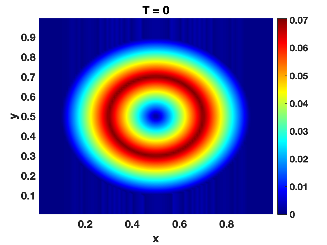
Figure 3: Pcolor plots of the initial Mach number profile for the vortex problem

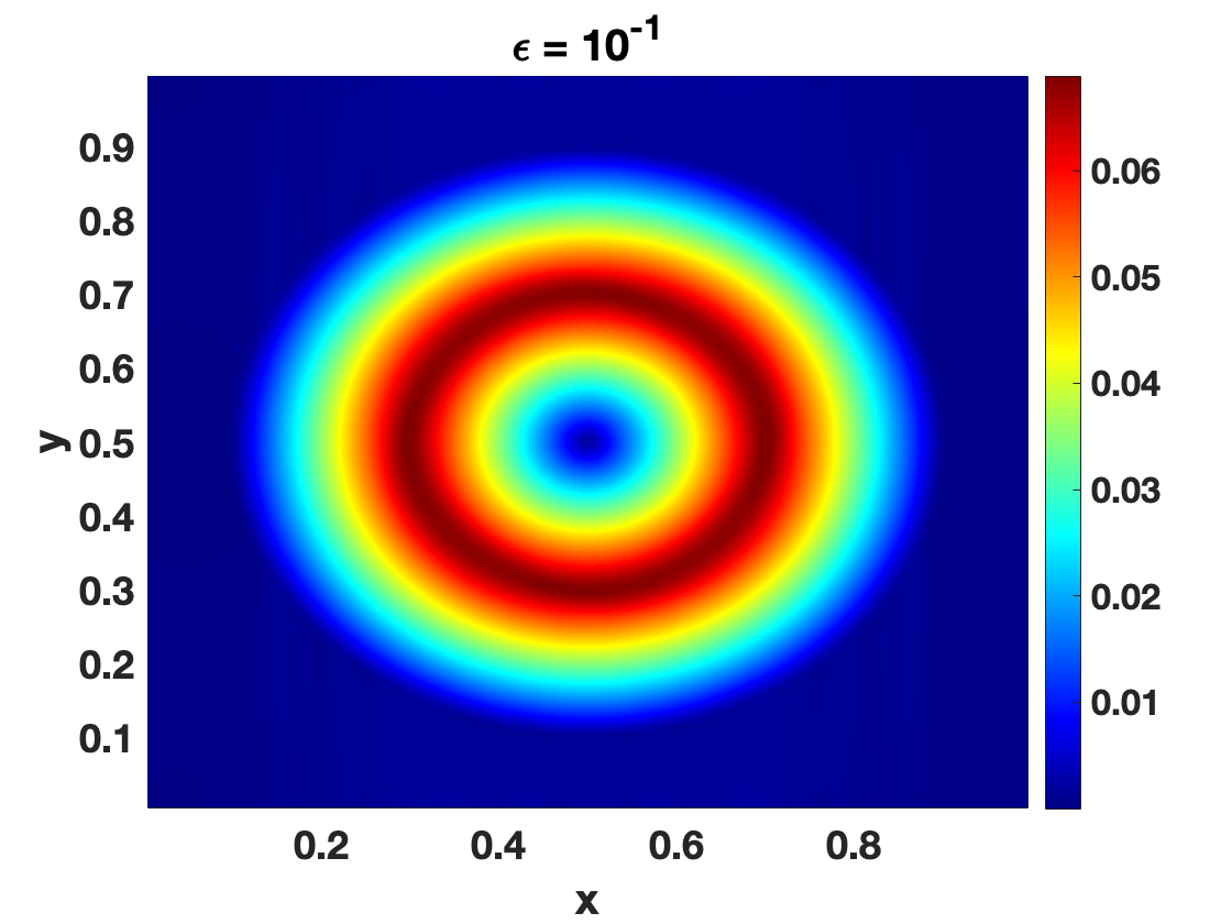
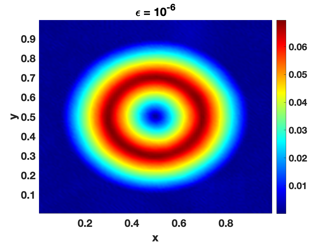
Figure 4: Pcolor plots of the Mach number profile for the vortex problem at time $t=1.0$ for $\varepsilon\in\{10^{-1},10^{-2},\ldots,10^{-6}\}$

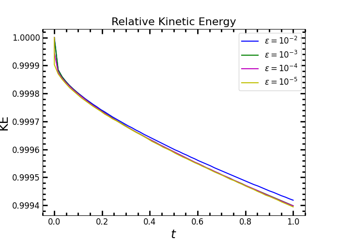
Figure 5: Relative Kinetic energy dissipation plot for the vortex problem

Figure 5 shows the kinetic energy dissipation plots for varied values of $\varepsilon$. We observe that the dissipation is independent of $\varepsilon$. Moreover, the numerical is capable to maintain almost a constant kinetic energy as the dissipation is of the order of $\mathcal{O}(10^{-4})$, which quite minuscule.

7 Conclusions

In this paper we have presented a novel additive IMEX-RK scheme for the low Mach regime of Euler equations with isentropic pressure law. The scheme hinges on a splitting of the momentum flux which is realised by adding and subtracting the constant density incompressibility constraint from the momentum flux. The scheme is linearly implicit. The time semi-discrete scheme is shown to be AP. A space time fully discrete finite volume which based on a combination of Rusanov fluxes and central differencing is implemented. The results of the numerical case studies show the uniform accuracy of the newly developed scheme with respect to the Mach number $\varepsilon$.

References

- [1] K. R. Arun and M. Kar, An energy stable well-balanced scheme for the barotropic euler system with gravity under the anelastic scaling, (2024), https://arxiv.org/abs/2405.00559, https://arxiv.org/abs/2405.00559.
- [2] K. R. Arun and S. Samantaray, Asymptotic preserving low Mach number accurate IMEX finite volume schemes for the isentropic Euler equations, J. Sci. Comput., 82 (2020), pp. Art. 35, 32, https://doi.org/10.1007/s10915-020-01138-8, https://doi.org/10.1007/s10915-020-01138-8.
- [3] U. M. Ascher, S. J. Ruuth, and R. J. Spiteri, Implicit-explicit Runge-Kutta methods for time-dependent partial differential equations, Appl. Numer. Math., 25 (1997), pp. 151–167, https://doi.org/10.1016/S0168-9274(97)00056-1, http://dx.doi.org/10.1016/S0168-9274(97)00056-1. Special issue on time integration (Amsterdam, 1996).
- [4] G. Bispen, K. R. Arun, M. Lukáčová-Medvid’ová, and S. Noelle, IMEX large time step finite volume methods for low Froude number shallow water flows, Commun. Comput. Phys., 16 (2014), pp. 307–347, https://doi.org/10.4208/cicp.040413.160114a, https://doi.org/10.4208/cicp.040413.160114a.
- [5] G. Bispen, M. Lukáčová-Medviďová, and L. Yelash, Asymptotic preserving IMEX finite volume schemes for low Mach number Euler equations with gravitation, J. Comput. Phys., 335 (2017), pp. 222–248, https://doi.org/10.1016/j.jcp.2017.01.020, https://doi.org/10.1016/j.jcp.2017.01.020.
- [6] S. Boscarino, J.-M. Qiu, G. Russo, and T. Xiong, A high order semi-implicit IMEX WENO scheme for the all-Mach isentropic Euler system, J. Comput. Phys., 392 (2019), pp. 594–618, https://doi.org/10.1016/j.jcp.2019.04.057, https://doi.org/10.1016/j.jcp.2019.04.057.
- [7] F. Cordier, P. Degond, and A. Kumbaro, An asymptotic-preserving all-speed scheme for the Euler and Navier-Stokes equations, J. Comput. Phys., 231 (2012), pp. 5685–5704, https://doi.org/10.1016/j.jcp.2012.04.025, http://www.sciencedirect.com/science/article/pii/S0021999112002069.
- [8] P. Degond, Asymptotic-preserving schemes for fluid models of plasmas, in Numerical models for fusion, vol. 39/40 of Panor. Synthèses, Soc. Math. France, Paris, 2013, pp. 1–90.
- [9] P. Degond and M. Tang, All speed scheme for the low Mach number limit of the isentropic Euler equations, Commun. Comput. Phys., 10 (2011), pp. 1–31.
- [10] S. Dellacherie, Analysis of Godunov type schemes applied to the compressible Euler system at low Mach number, J. Comput. Phys., 229 (2010), pp. 978–1016, https://doi.org/10.1016/j.jcp.2009.09.044, http://dx.doi.org/10.1016/j.jcp.2009.09.044.
- [11] G. Dimarco, R. Loubère, and M.-H. Vignal, Study of a new asymptotic preserving scheme for the Euler system in the low Mach number limit, SIAM J. Sci. Comput., 39 (2017), pp. A2099–A2128, https://doi.org/10.1137/16M1069274, https://doi.org/10.1137/16M1069274.
- [12] H. Guillard and C. Viozat, On the behaviour of upwind schemes in the low Mach number limit, Comput. & Fluids, 28 (1999), pp. 63–86, https://doi.org/10.1016/S0045-7930(98)00017-6, http://dx.doi.org/10.1016/S0045-7930(98)00017-6.
- [13] E. Hairer and G. Wanner, Solving ordinary differential equations. II, vol. 14 of Springer Series in Computational Mathematics, Springer-Verlag, Berlin, second ed., 1996, https://doi.org/10.1007/978-3-642-05221-7, https://doi.org/10.1007/978-3-642-05221-7. Stiff and differential-algebraic problems.
- [14] S. Jin, Efficient asymptotic-preserving (AP) schemes for some multiscale kinetic equations, SIAM J. Sci. Comput., 21 (1999), pp. 441–454, https://doi.org/10.1137/S1064827598334599, http://epubs.siam.org/doi/abs/10.1137/S1064827598334599, https://arxiv.org/abs/http://epubs.siam.org/doi/pdf/10.1137/S1064827598334599.
- [15] S. Jin, Asymptotic preserving (AP) schemes for multiscale kinetic and hyperbolic equations: a review, Riv. Math. Univ. Parma (N.S.), 3 (2012), pp. 177–216.
- [16] C. A. Kennedy and M. H. Carpenter, Additive Runge-Kutta schemes for convection-diffusion-reaction equations, Appl. Numer. Math., 44 (2003), pp. 139–181, https://doi.org/10.1016/S0168-9274(02)00138-1, https://doi.org/10.1016/S0168-9274(02)00138-1.
- [17] R. Klein, Semi-implicit extension of a Godunov-type scheme based on low Mach number asymptotics. I. One-dimensional flow, J. Comput. Phys., 121 (1995), pp. 213–237, https://doi.org/10.1016/S0021-9991(95)90034-9, http://dx.doi.org/10.1016/S0021-9991(95)90034-9.
- [18] S. Noelle, G. Bispen, K. R. Arun, M. Lukáčová-Medviďová, and C.-D. Munz, A weakly asymptotic preserving low Mach number scheme for the Euler equations of gas dynamics, SIAM J. Sci. Comput., 36 (2014), pp. B989–B1024, https://doi.org/10.1137/120895627, https://doi.org/10.1137/120895627.
- [19] L. Pareschi and G. Russo, Implicit-explicit Runge-Kutta schemes for stiff systems of differential equations, in Recent trends in numerical analysis, vol. 3 of Adv. Theory Comput. Math., Nova Sci. Publ., Huntington, NY, 2001, pp. 269–288.
- [20] H. Zakerzadeh and S. Noelle, A note on the stability of implicit-explicit flux-splittings for stiff systems of hyperbolic conservation laws, Commun. Math. Sci., 16 (2018), pp. 1–15, https://doi.org/10.4310/CMS.2018.v16.n1.a1, https://doi.org/10.4310/CMS.2018.v16.n1.a1.