Measuring the speed of light with cosmological observations: current constraints and forecasts

Abstract

We measure the speed of light with current observations, such as Type Ia Supernova, galaxy ages, radial BAO mode, as well as simulations of future redshift surveys and gravitational waves as standard sirens. By means of a Gaussian Process reconstruction, we find that the precision of such measurements can be improved from roughly 6% to 1.5-2%, in light of these forthcoming observations. This result demonstrates that we will be able to perform a cosmological measurement of a fundamental physical constant with unprecedented precision, which will help us underpinning if its value is truly consistent with local measurements, as predicted by the standard model of Cosmology.

I Introduction

Since the late 1990s, the Standard Cosmological Model (SCM) has been described by the flat $\Lambda$CDM model Riess ; Perlmutter , which states that the Universe is dominated by cold dark matter as the responsible for structure formation and galaxy dynamics, and by the cosmological constant $\Lambda$ as the responsible for the accelerated expansion of the Universe at late times. The framework of the SCM provides a series of successful predictions, such as recent observations of the Cosmic Microwave Background (CMB) Aghanim , luminosity distances of Type Ia Supernovae (SNe) SCOLNIC , as well as galaxy clustering and weak lensing Alam ; Asgari ; Abbott ; Secco , which validate the SCM as the model that best describes the observed data with great precision.

However, we can mention some unresolved problems in relation to the SCM, such as problems of primordial singularity and cosmic coincidence. We also have tensions in measurements of some cosmological parameters, e.g. the tension of $\sim 5\sigma$ between the Hubble Constant $H_{0}$ measured in the late- and early-time Universe with SNe and CMB, respectively, being one of most evident at the current moment DiValentino – see also Perivolaropoulos for a broad review on cosmological tensions. Recently, the first data release of the DESI telescope showed that there could be an evolution of the dark energy equation of state, thus hinting at a possible breakdown of the cosmological constant paradigm DESI . In such a scenario, it is necessary to propose and test alternative models, besides revisiting the SCM fundamentals, since further evidence for departures of the SCM predictions would suggest new physics at play, and require a complete reformulation of its panorama. The validity of two fundamental pillars of the SCM, namely the Cosmological Principle and General Relativity as a theory of gravity on large scales, have been confirmed in recent works, although some results may affirm the opposite Perivolaropoulos .

A possible route to propose alternative models to the SCM consists on studying the variability of the fundamental constants of nature, as discussed in Dirac ; Uzan1 ; Uzan2 ; Martins . Experiments with this purpose have been carried out for centuries on Earth and in the Solar System to measure the values of fundamental constants, obtaining zero results for their variations and with supreme precision in their measurements. However, cosmological tests of the consistency of fundamental constants are very scarce and less precise, due to the difficulty in obtaining cosmological data at high redshifts that would make their achievements possible. At this point, it is crucial to take care when leveraging such models, as they can trigger additional problems in the physical laws under which these physical constants were constructed. For example, models that assume a variable speed of light (VSL) must reproduce the success of the Special Theory of Relativity in explaining at least thermodynamics and electromagnetism. Some of these models meet these requirements and can provide viable solutions to SCM problems Moffat1 ; Barrow1 ; Albrecht ; Barrow2 ; Barrow3 ; Clayton1 ; Avelino ; Clayton2 ; Bassett ; Magueijo1 ; Clayton3 ; Magueijo2 ; Ellis1 ; Ellis2 ; Magueijo3 ; Cruz1 ; Moffat2 ; Franzmann ; Cruz2 ; Costa ; Gupta ; Lee1 .

Driven by this reason, some recent studies searched for possible evidence of VSL model, and carried out speed of light measurements with cosmological observations, mostly obtaining null evidence for the former, and results in good concordance with the measurements in local laboratories for the latter Balcerzak1 ; Zhang1 ; Balcerzak2 ; Zhang2 ; SALZANO ; VSalzano ; Cai ; Balcerzak3 ; SCao1 ; Dabrowski ; Salzano1 ; Guedes ; ZouDeng ; Huerta ; SCao2 ; Wang ; AAlbert ; Pan ; Mendonca ; GC ; Lee6 ; Mukherjee1 ; Liu ; Lee7 ; Cuzinatto ; Zhang . For instance, in GC , the authors used data from the Pantheon SNe compilation, besides measurements of the Hubble parameter obtained through the differential ages galaxies and the radial mode of baryon acoustic oscillations (BAO), to measure the speed of light by means of the methodology proposed by VSalzano . These analyses were done using Gaussian Processes, i.e., a non-parametric reconstruction method – thus, no cosmological model is assumed a prori – resulting in measurements of $\simeq 5\%$ precision at $z=1.4-1.6$. Although these results agree within $2\sigma$ confidence level with typical speed of light measurements here on Earth, we should note that the availability of cosmological data at such redshift range is quite limited. Hence, the precision of those tests are inevitably affected by this fact, not to mention that some of the cosmological data could be biased towards the SCM scenario.

Hence, considering the caveats of the SCM, as previously discussed, and considering the importance of performing cosmological measurements of the fundamental constants in this context, we forecast the precision of speed of light measurements that can be reached by future cosmological observations. We produce simulations of the Hubble parameter measurements expected from upcoming redshift surveys, as well as luminosity distance measurements that are expected from future observations of gravitational wave (GW) events, by means of the standard siren method. Although the speed of the GW event GW170817 was precisely measured as being the same as the speed of light, which confirms the predictions of general relativity theory Flanagan , here we pursue a different approach to measure the speed of light from GW, as carried out in VSalzano ; GC , given the advent of the standard siren measurements that upcoming GW experiments shall provide. Our main goal is to assess the precision that those speed of light measurements can be improved, when compared to current constraints.

The paper is organized as follows: in section 2, we describe the theoretical framework, followed by section 3, in which we present the data and simulations, section 4 presents our results. Finally, section 5 is dedicated to discussion and concluding observations.

II Theoretical Framework

In order to obtain a cosmological measurement of the speed of light, we adopt the method proposed by SALZANO . This method consists of assuming a flat Universe described by the Friedmann-Lemaître-Robertson-Walker (FLRW) metric, so that the angular diameter distance is given by by the equation

$$D_{A}(z)=\frac{1}{(1+z)}\int_{0}^{z}\frac{cdz}{H(z)}\,,$$ (1)

where $c=c(z)$ is the speed of light – here, written as a function of redshift for the sake of convenience – and $H(z)$ is the Hubble parameter that gives the expansion rate of the Universe at a given redshift $z$.

Thus, deriving Eq. (1) with respect to redshift, we have

$$\frac{\partial}{\partial z}[(1+z)D_{A}(z)]=\frac{c(z)}{H(z)}\,,$$ (2)

so we can write $c(z)$ as

$$c(z)=H(z)[(1+z)D^{\prime}_{A}(z)+D_{A}(z)]\,,$$ (3)

where $D^{\prime}_{A}(z)$ denotes the first derivative of the angular diameter distance in relation to redshift. Also, we can obtain the uncertainties through an error propagation, given as follows,

$$\sigma^{2}_{c(z)}=H^{\prime}(z)[(1+z)D_{A}^{\prime}(z)+D_{A}(z)]\sigma^{2}_{H(z)}+H(z)[(1+z)D_{A}^{\prime\prime}(z)+D_{A}(z)]\sigma^{2}_{D_{A}^{\prime}(z)}+$$ (4)

$$+H(z)[(1+z)D_{A}^{\prime}(z)]\sigma^{2}_{D_{A(z)}}\,.$$

In the SCM scenario, $D_{A}(z)$ is expected to reach its maximum value at around $z\sim 1.4-1.6$, depending on the cosmological parameters of the model, for instance, the matter density parameter and the Hubble Constant. Therefore, when we take the first derivative of the angular diameter distance at this maximum redshift ($z_{m}$), its value will be zero (i.e. $D_{A}^{\prime}(z_{m})=0$). So, at such redshift, Eq. (3) can be rewritten as

$$c(z_{m})=D_{A}(z_{m})H(z_{m})\,,$$ (5)

once more, we can obtain the uncertainties through an error propagation given as follows,

$$\sigma^{2}_{c(z_{m})}=\left(H(z)\sigma_{D_{A}(z)}\right)^{2}+\left(D_{A}(z)\sigma_{H(z)}\right)^{2}\,.$$ (6)

Therefore, we can arrive at an expression for the speed of light at such a redshift that depends only on the angular diameter distance and the Hubble parameter, allowing us to measure it with higher precision because it does not depend on their respective derivatives, which suffer from smearing effect – and thus much larger uncertainties. It is worthful to notice that because there is a degeneracy between a variable speed of light and cosmic curvature, we note that this method is only valid for flat FLRW models VSalzano ; Dabrowski . Still, recent measurements of the curvature of the Universe are in excellent agreement with a flat Universe, so we can safely make this assumption Aghanim ; SCOLNIC ; Alam ; Asgari ; Abbott ; Secco ; DESI .

III Data and simulations

We use 1701 luminosity distance measurements of Type Ia Supernovae (SNe) from the Pantheon+ and SH0ES compilation, and 48 Hubble parameter measurements $H(z)$ obtained through differential galaxy ages and the radial mode of baryon acoustic oscillations (BAO) MAGANA ; MORESCO , as our current cosmological data-sets. In addition, we produce simulations of future cosmological observations, such as 1000 luminosity distance measurements from gravitational wave events (GW) as standard sirens, as expected by experiments such as LIGO LIGO and Einstein Telescope (ET) ET , along with 30 $H(z)$ measurements that are expected for the new generation of redshift surveys, as the case of J-PAS J-PAS1 , detailed as follow:

III.1 Type Ia Supernovae

The latest SN compilation, namely the Pantheon+SH0ES data-set PantheonPlus1 (see also PantheonPlus2 ; SH0ES ), provides 1701 light curve measurements of 1550 SN objects in the redshift interval $0.001<z<2.26$. Hence, we have 1701 measurements of SN apparent magnitudes, $m_{B}$, which can be combined with the determination of the SN absolute magnitude given by SCOLNIC

$$M_{B}=-19.25\pm 0.03\,.$$ (7)

We can obtain the luminosity distances through

$$D_{L}(z)=10^{\frac{m_{B}(z)-M_{B}-25}{5}}\,.$$ (8)

Then we can convert the luminosity distances into angular diameter distances by means of the cosmic distance duality relation (CDDR), which reads

$$D_{A}(z)=D_{L}(z)(1+z)^{-2}\,.$$ (9)

This relationship is valid for all models based on Riemannian geometry, being independent of Einstein’s field equations, the FLRW metric, or the nature of dark matter and dark energy. The violation of the CDDR would only occur in the case of geometry non-Riemannian, the presence of a source of cosmic opacity in the Universe, or variations in fundamental physics, such as the Equivalence Principle and the fine structure constant. Nonetheless, recent works showed that the CDDR is validated through a variety of cosmological observations and approaches, as in Goncalves ; Mukherjee2 ; Bora ; Renzi ; Tonghua .

III.2 Gravitational Waves

In order to obtain the simulated data sets of gravitational waves, we assume that the sources of the events are mergers of Neutron Stars-Black Hole (NS-BH) or Neutron Stars-Neutron Stars (NS-NS) binaries. They obey a redshift distribution given by

$$P(z)\propto\frac{4\pi D_{c}^{2}R(z)}{H(z)(1+z)},$$ (10)

where $d_{c}$ is the comoving distance and $H(z)$ is the Hubble parameter WZhao . Both quantities are defined from a fiducial cosmology by assuming a flat $\Lambda$CDM model with $H^{\rm fid}_{0}=73.30\pm 1.04\,\mathrm{km\,s}^{-1}\,\mathrm{Mpc}^{-1}$, $\Omega^{\rm fid}_{\rm m}=0.334\pm 0.018$ and $\Omega^{\rm fid}_{\Lambda}=1-\Omega_{\rm m}$, consistent with the Pantheon+SH0ES best-fit PantheonPlus1 .

The factor $R(z)$ describes the evolution of the star formation rate CCutler and it has a specific functional form for each gravitational wave source given by

$$R(z)=\begin{cases}1+2z\text{,}&z\leq 1\\ \frac{3}{4}(5-z)\text{,}&1<z<5\\ 0\text{,}&z\geq 5\end{cases}$$ (11)

From the probability distribution for each gravitational source we randomly pick 1000 points in the redshift range $0<z<2.36$. We then obtain the luminosity distance ($D_{L}$) at those redshift with the fiducial model, and we perform a Monte Carlo simulation by assuming a gaussian distribution centered on these fiducial $D_{L}$. The standard deviation ($\sigma_{D_{L}}$) is related with an instrumental error ($\sigma_{D_{L}^{inst}}$) that can be obtained via a Fisher Matrix analysis and combined with an additional error from weak lensing ($\sigma_{D_{L}^{WL}}$) JFZhang ,

$$\sigma_{D_{L}}=\sqrt{\left(\sigma_{D_{L}^{inst}}\right)^{2}+\left(\sigma_{D_{L}^{WL}}\right)^{2}}=\sqrt{\left(\frac{2D_{L}}{\rho}\right)^{2}+\left(0.05zD_{L}\right)^{2}}.$$ (12)

The parameter $\rho$ represents the signal-to-noise ratio of the detection (SNR) and is directly related to the amplitude of the gravitational wave ($A$), the interferometer antenna pattern ($F$), and the power spectrum density ($PSD$) JFZhang .

We simulate the data from two interferometer configurations, with its specific $F$ and $PSD$. The first configuration is defined by assuming a perpendicular interferometer (as the LIGO collaboration), in this case we have the antenna pattern given by

$$F^{2}=\frac{1}{4}(1+cos^{2}(\theta))^{2}cos^{2}(2\phi)+cos^{2}(\theta)sen^{2}(2\phi),$$ (13)

with the angles $\theta$ and $\phi$ varying in the range $[0,\frac{1}{2}\pi]$ BSchutz . Moreover, the Power Spectrum Density is given by

$$\frac{S_{h}(x)}{S_{0}}=(4.49x)^{-56}+0.16x^{-4.52}+0.52+0.32x^{2},$$ (14)

with $S_{0}/Hz^{-1}=9.0\times 10^{-46}$, $f_{s}/Hz=40$ and $f_{0}/Hz=150$ BSathyaprakash .

The second interferometer configuration has a triangular pattern (as the Einstein Telescope). Besides the difference in angles, it also has a difference in sensitivity. In this case the antenna pattern is given by

$$F^{2}=\frac{9}{256}\left(35+28cos(2\theta)+cos(4\theta)\right),$$ (15)

with the angles $\theta$ varying between [0,$\pi$] WZhao . Its Power Spectrum Density is given by

$$Sh(f)=S_{0}\left[x^{p_{1}}+a_{1}x^{p_{2}}+a_{2}\frac{1+b_{1}x+b_{2}x^{2}+b_{3}x^{3}+b_{4}x^{4}+b_{5}x^{5}+b_{6}x^{6}}{1+c_{1}x+c_{2}x^{2}+c_{3}x^{3}+c_{4}x^{4}}\right]$$ (16)

where $x=f/f_{0}$ with $f_{0}=200Hz$ and $S_{0}=1.449\times 10^{-52}Hz^{-1}$. The other parameters are as follows: $p_{1}=-4.05$, $p_{2}=-0.69$, $a_{1}=185.62$, $a_{2}=232.56$, $b_{1}=31.18$, $b_{2}=-64.72$, $b_{3}=52.24$, $b_{4}=-42.16$, $b_{5}=10.17$, $b_{6}=11.53$, $c_{1}=13.58$, $c_{2}=-36.46$, $c_{3}=18.56$, $c_{4}=27.43$ WZhao .

The amplitude of the wave is needed to calculate the SNR, and it is given by WZhao

$$A^{2}=\frac{4}{D_{L}^{2}}\left(\frac{5\pi}{96}\right)\pi^{-\frac{7}{3}}\left(M_{c}G(1+z)\right)^{\frac{5}{3}},$$ (17)

the $M_{c}$ stands for the chirp mass of the gravitational wave, which depends on the masses of the two merging objects, whether neutron stars (NS) or black holes (BH). The formula for the chirp mass is given by

$$M_{c}=\mu^{\frac{3}{5}}M^{\frac{2}{5}}=\frac{(m_{1}m_{2})^{\frac{3}{5}}}{(m_{1}+m_{2})^{\frac{1}{5}}}$$ (18)

we define the components masses of the binary system $m_{1}$ and $m_{2}$, then $M=m_{1}+m_{2}$ as the total mass and $\mu=(m_{1}m_{2})/{M}$ as the reduced mass MMaggiore . The mass ranges for each component are $[1,3]M_{\odot}$ for neutron stars and $[5,35]M_{\odot}$ for black holes, with both obeying the respective probability density functions PLandry ; WFarr .

III.3 Hubble Parameter

As for our sample of $H(z)$, we adopt a compilation of 30 measurements obtained from differential galaxy ages, and 18 measurements from the radial BAO mode. This data-set is hereafter named CC, as they are commonly referred in the literature as cosmic chronometers. Instead of using the actual observational measurements, we replace them by a realization of the flat $\Lambda$CDM model, i.e., $H^{\rm obs}(z)\rightarrow\mathcal{N}(H^{\rm fid}(z),\sigma_{H^{\rm obs}(z)})$, so that the Hubble parameter follows the Friedmann equation

$$\left[\frac{H^{\rm fid}(z)}{H^{\rm fid}_{0}}\right]^{2}=\Omega^{\rm fid}_{\rm m}(1+z)^{3}+\Omega^{\rm fid}_{\Lambda}\,,$$ (19)

and again, we assume a fiducial flat $\Lambda$CDM model consistent with the Pantheon+SH0ES best-fit as Section II.B PantheonPlus1 . By the same token, we simulate future $H(z)$ measurements expected from ongoing redshift surveys, like J-PAS. We produce 30 data points from a realization of the $\Lambda$CDM fiducial model, as done for the observational CC data-set, but assuming that the $H(z)$ uncertainties should follow the values shown in Fig. 15 of J-PAS2 for a J-PAS 8500 degree² configuration. Also, we assume that these data points should follow a redshift distribution $P(z)$ in the interval $0.3<z<2.5$, as given by Wang20 ; Bengaly23

$$P(z;\;k,\theta)=z^{k-1}\frac{e^{-z/\theta}}{\theta^{k}\Gamma(k)}\;,$$ (20)

where we fix $\theta$ and $k$ to their respective best fits to the real data, i.e., $\theta_{\rm bf}=0.647$ and $k=1.048$.

IV Results

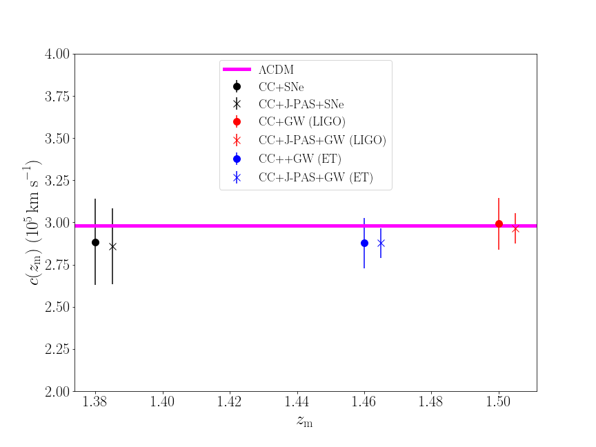
Figure 1: Upper panel: $c(z_{m})$ measurements, as a function of $z_{m}$, obtained assuming the Squared Exponential GP kernel from the following combination of data-sets: CC+SNe (black circle), CC+GW from LIGO (red circle), CC+GW from ET (blue circle). The combination of the same data-sets with the $H(z)$ from J-PAS are denoted by black, red and blue stars, respectively. Lower panel: Same as left panel, but rather assuming the Matérn(7/2) kernel. The uncertainties in all cases correspond to the $2\sigma$ CL, and the magenta horizontal line represent the value predicted by the $\Lambda$CDM scenario.

In order to obtain $c(z_{m})$ and its respective uncertainty, as in Eq. 5 and 6, respectively, we need to carry out an interpolation across the redshift range that is covered by those data-sets. So, we follow the approach of GC , and reconstruct $\{D_{\text{A}}(z)$, $H(z)\}$, as well as their respective derivatives $\{D^{\prime}_{\text{A}}(z)$, $H^{\prime}(z)\}$, from those datasets using a non-parametric approach – namely the Gaussian Processes (GP) method, as in the GAPP package MSeikel . We assume two kernels to perform these reconstructions, i.e., Squared Exponential (hereafter SqExp) and Matérn(7/2) (hereafter Mat72), for $n=250$ bins within the redshift range $0.01<z<2.5$, in which we optimize the GP hyperparameters in both cases. So we can obtain $z_{m}$ at the point where the reconstructions yield $D^{\prime}_{A}\simeq 0$, and then calculate $c(z_{m})$ and $\sigma_{c(z_{m})}$ according to Eqs. (5) and (6). More details on the reconstructions obtained for each case are shown in the Appendix.

Table 1: Results for the $c(z_{\rm m})$ measurements assuming the Squared Exponential GP kernel. The first column displays the combination of data-sets, the second column shows the reconstructed $z_{\rm m}$ value, the third column provides the $c(z_{\rm m})$ measurements and their uncertainties in $1\sigma$ CL, in units of $10^{5}\,\mathrm{km\,s}^{-1}$, and the fourth column gives their relative uncertainty, in percent.

data-sets (CC+)	$z_{\rm m}$	$c(z_{\rm m})\pm\sigma_{c(z_{\rm m})}$	uncertainty (%)
+SNe (Pantheon+SH0ES)	$1.77$	$3.319\pm 0.210$	$6.25$
+GW (LIGO)	$1.64$	$3.217\pm 0.067$	$2.08$
+GW (ET)	$1.63$	$3.140\pm 0.066$	$2.10$
data-sets (CC+JPAS+)	$z_{\rm m}$	$c(z_{\rm m})\pm\sigma_{c(z_{\rm m})}$	uncertainty (%)
+SNe (Pantheon+SH0ES)	$1.77$	$3.293\pm 0.203$	$6.16$
+GW (LIGO)	$1.64$	$3.190\pm 0.044$	$1.38$
+GW (ET)	$1.63$	$3.114\pm 0.043$	$1.38$

Table 2: Same as Table 1, but rather assuming the Matérn(7/2) kernel.

data-sets (CC+)	$z_{\rm m}$	$c(z_{\rm m})\pm\sigma_{c(z_{\rm m})}$	uncertainty (%)
+SNe (Pantheon+SH0ES)	$1.38$	$2.884\pm 0.128$	$4.45$
+GW (LIGO)	$1.50$	$2.992\pm 0.077$	$2.59$
+GW (ET)	$1.46$	$2.877\pm 0.074$	$2.58$
data-sets (CC+JPAS+)	$z_{\rm m}$	$c(z_{\rm m})\pm\sigma_{c(z_{\rm m})}$	uncertainty (%)
+SNe (Pantheon+SH0ES)	$1.38$	$2.859\pm 0.112$	$3.91$
+GW (LIGO)	$1.50$	$2.965\pm 0.045$	$1.52$
+GW (ET)	$1.46$	$2.851\pm 0.043$	$1.51$

Figure 1 displays all these results in black (CC+SNe), blue (CC+GW from LIGO), and red (CC+GW from ET) circles, whereas the crosses of the same color code represent the combination of the corresponding data-sets with the J-PAS simulations, albeit at a $2\sigma$ CL uncertainty for the sake of enhancing visualization. The difference between the left and the right panel is the GP kernel under assumption – the left panel shows the results obtained from the SqExp kernel reconstructions, while the right panel displays the Mat72 case. The horizontal line represents the locally measured $c$, i.e., $c=2.998\times 10^{5}\,\mathrm{km\,s}^{-1}$. So we can clearly see that our results are in agreement with this local value, and they are consistent with each other, with the results obtained from Mat72 being slightly more compatible with the local measurements.

In tables 1 and 2, we present the results obtained from the GP reconstructions assuming, respectively, the SqExp and Mat72 kernels. We can see in the top of both tables that the combination of current CC+SNe data provides a measurement of $c(z_{\text{m}})$ with a precision of $\sim 6.2\%$ (SqExp), and $\sim 4.5\%$ (Mat72), whereas combining CC with GW simulations from ET and LIGO, the precision is slightly improved – $\sim 2\%$ (SqExp), and $\sim 2.5\%$ (Mat72). Also, we note that the results obtained by LIGO and ET are totally consistent with each other, to a sub-percent level. When we include the simulated J-PAS $H(z)$ measurements to the CC data-set, and combine it with the SN and GW data, as shown in the bottom of both tables, we find that the precision of the $c(z_{\text{m}})$ measurement is only mildly improved in the former case, but significantly improved for the latter, reaching $\sim 1.4\%$ (SqExp), and $\sim 1.5\%$ (Mat72).

These results demonstrate that future observational data have the capability of improving the measurements of the speed of light to a few percent level, and therefore we will be able determine with much higher precision whether its value actually agrees with the measurements carried out in local laboratories, as predicted from the standard cosmological model, or whether there is any hint at new physics if found otherwise.

V Conclusions

Performing cosmological measurements of the fundamental physical constants is of great importance, as any statistically significant departure from local measurements would immediately require a reformulation of the standard cosmological model. In this work, we measure the speed of light $c$ with Hubble parameter and angular diameter distance measurements from current data-sets, as obtained from a compilation of galaxy ages and radial baryon acoustic oscillations for the former, and Type Ia Supernova distances from Pantheon+SH0ES for the latter. We do so by performing a Gaussian Process reconstruction of such quantities, in order to avoid the assumption of a cosmological model. Then, we forecast the precision of such a measurement by simulating the same kind of data from upcoming galaxy redshift surveys, such as J-PAS, and from standard sirens from gravitational wave experiments, as in the cases of LIGO and the Einstein Telescope.

We obtained a significant improvement between the current and future constraints, reducing our uncertainties from $4-6\%$ to about $2-2.5\%$ when the gravitational wave simulations are considered, and to nearly $1.5\%$ when the simulated J-PAS measurements are taken into account as well, at redshifts around $1.4<z<1.8$. We noted that these figures hold regardless of the assumption on the reconstruction kernel, the number of bins for each reconstruction etc.

Our result show the capability of the upcoming generation of cosmological observations in terms of carrying out a powerful test of fundamental physics, as we found that such a combination of data-sets, along with the statistical approach herein deployed, will be able to provide a percent-level precision measurement of the speed of light at cosmological scales. Therefore, we will be able to verify if the speed of light at high redshift ranges – which corresponds to a Universe age of around $3.2-4.0$ Gyr – is actually consistent with local measurements with unprecedented precision, which will help determining the validity (or departure) of the standard model of Cosmology.

Acknowledgments: We thank to Jailson S. Alcaniz for valuable discussions. JS acknowleges financial support from Coordenação de Aperfeiçoamento de Pessoal de Nível Superior (CAPES). CB acknowledges financial support from Fundação à Pesquisa do Estado do Rio de Janeiro (FAPERJ) - Postdoc Recente Nota 10 (PDR10) fellowship. JM acknowledges financial support from Conselho Nacional de Desenvolvimento Científico e Tecnológico (CNPQ) - Undergraduate research fellowship. RSG thanks financial support from the Fundação de Amparo à Pesquisa do Estado do Rio de Janeiro (FAPERJ) grant SEI-260003/005977/2024 - APQ1.

Appendix A Gaussian Process Reconstructions

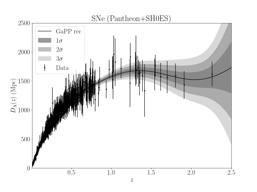
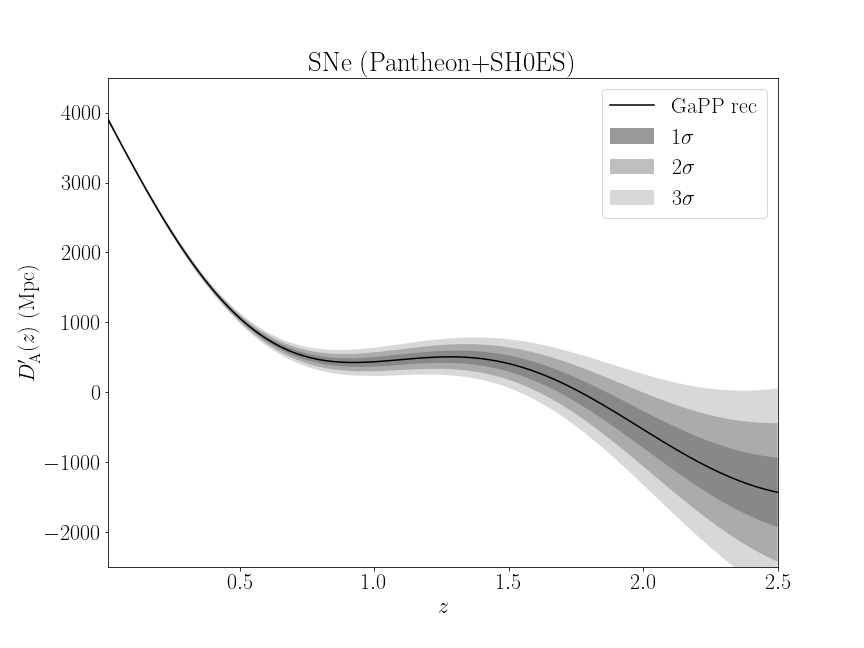
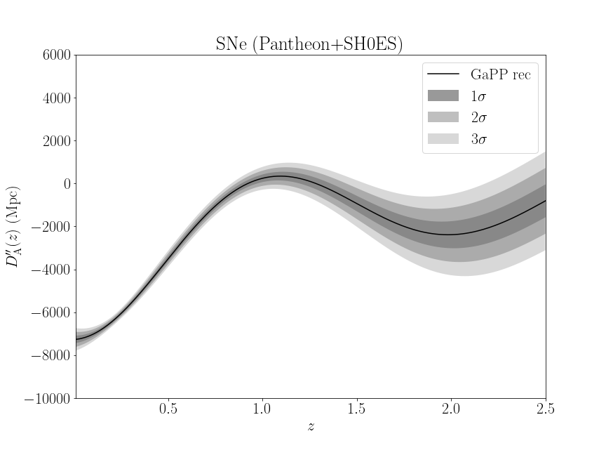
Figure 2: The top left panel shows the Gaussian Process reconstruction of the angular diameter distance, $D_{A}(z)$, as obtained by Eqs. (7) to (1), using the Pantheon+SH0ES Type Ia Supernova compilation. The top right panel displays the reconstruction of the first order derivative, $D_{A}^{\prime}(z)$, whereas the bottom central panel depicts the reconstruction of the second order derivative, $D_{A}^{\prime\prime}(z)$, still obtained from the same observational sample. The black dots with error bars in the $D_{A}(z)$ plot represent the observational data, and the gray curves denote the $1$, $2$, and $3\sigma$ confidence level of the reconstructions, respectively from the darker to the lighter shade. All reconstructions were performed assuming the Squared Exponential kernel.

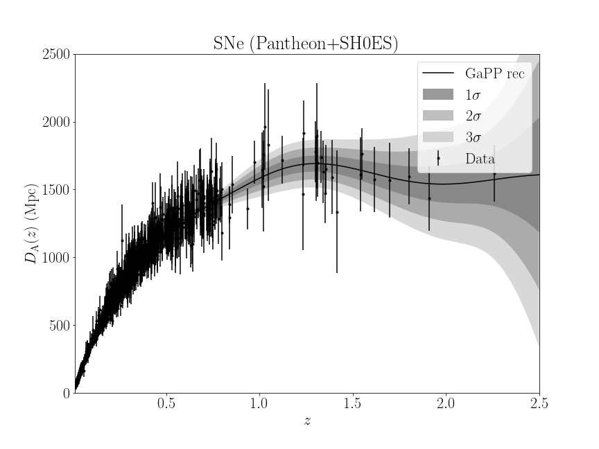
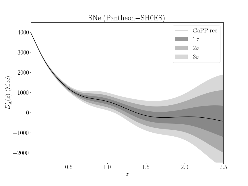
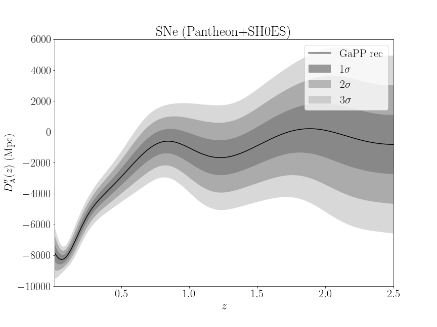
Figure 3: Same as Fig. 2, but assuming the Matérn(7/2) Gaussian Process kernel instead.

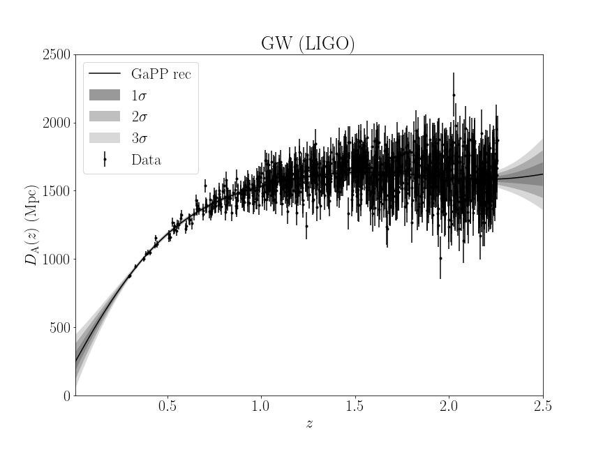
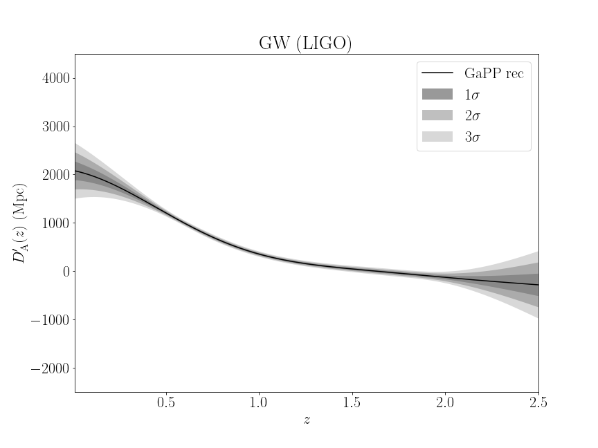
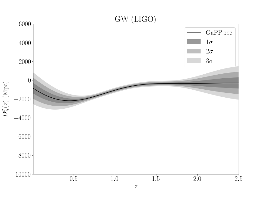
Figure 4: Same as Fig. 2, but valid for the simulated gravitational wave data-set assuming the LIGO interferometer specifications.

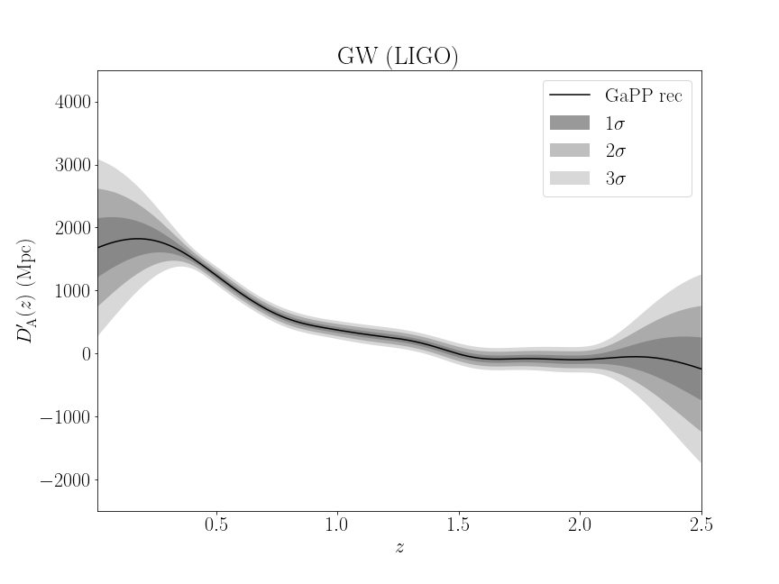
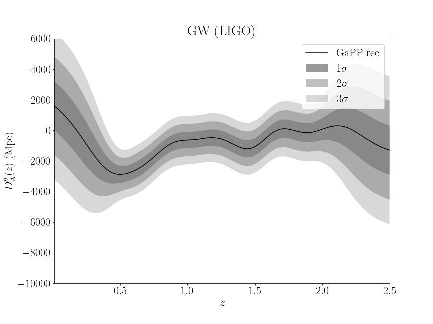
Figure 5: Same as Fig. 4, but assuming the Matérn(7/2) Gaussian Process kernel instead.

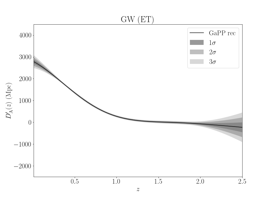
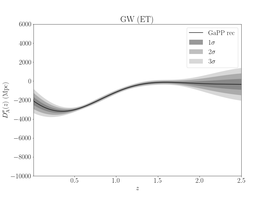
Figure 6: Same as Fig. 4, but valid for the simulated gravitational wave data-set assuming the Einstein Telescope specifications.

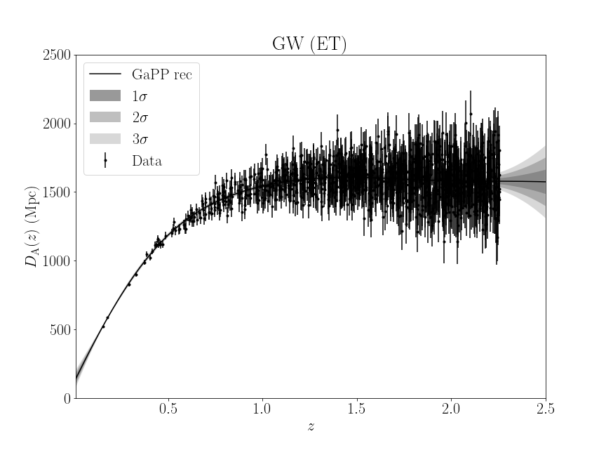
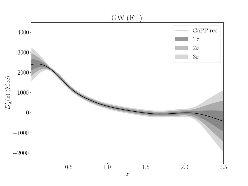
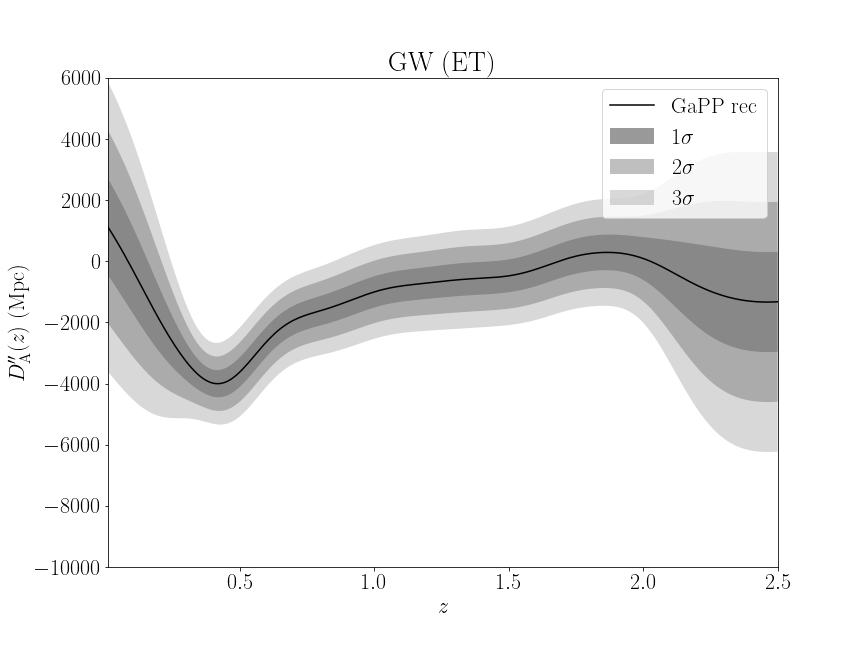
Figure 7: Same as Fig. 6, but assuming the Matérn(7/2) Gaussian Process kernel instead.

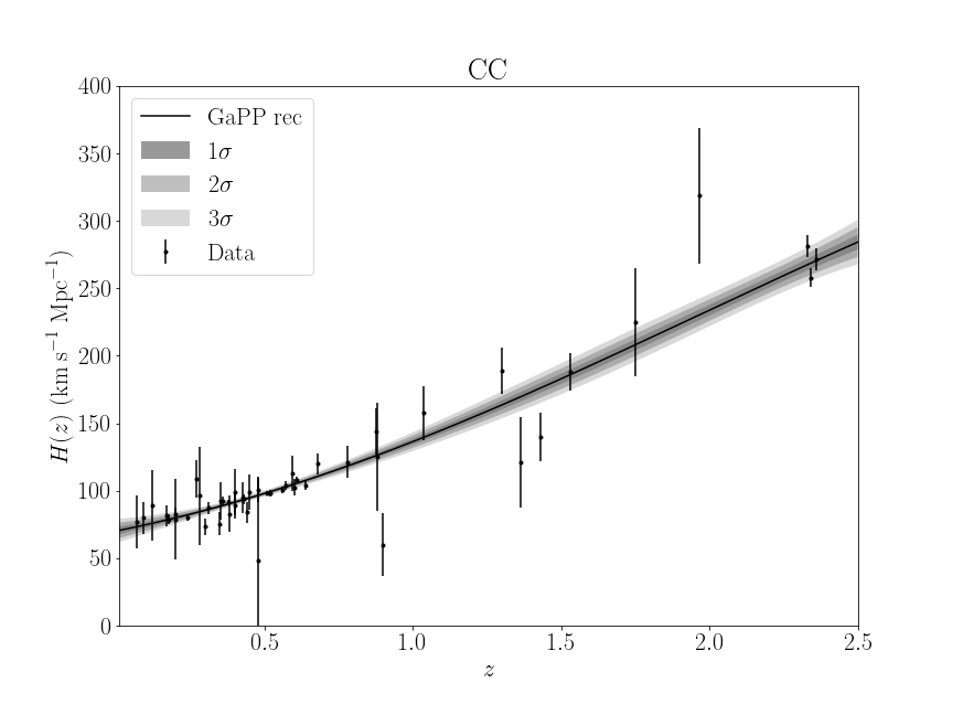
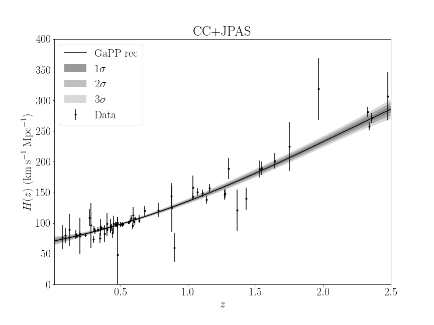
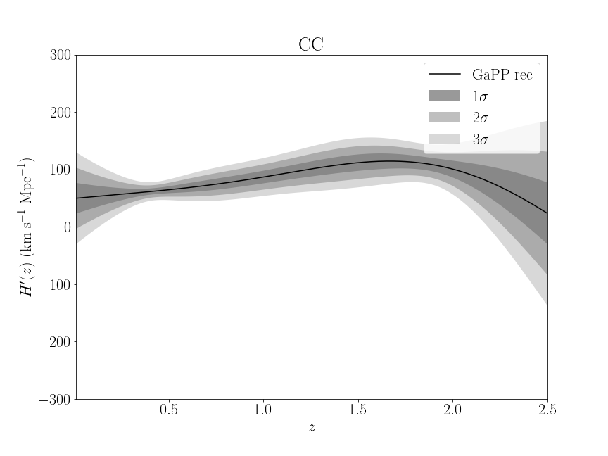
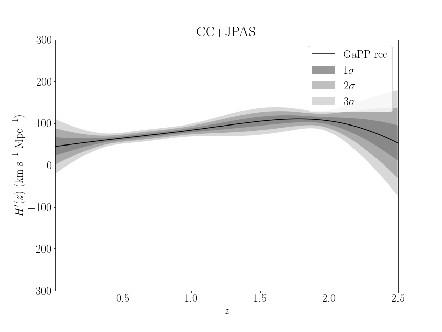
Figure 8: Top left panel: The reconstruction of the Hubble parameter, $H(z)$, obtained from the cosmic chronometer data-set. The black dots depict the data points with their respective uncertainties. Top right panel: Similar to the former, but rather for the cosmic chronometer combined with simulated J-PAS simulated data-set. Bottom left panel: The first derivative of the Hubble parameter, $H^{\prime}(z)$, from the cosmic chronometer sample alone. Bottom right panel: Similar to the previous plot, but for the cosmic chronometer with J-PAS combination. As in the previous plots, the gray curves denote the $1$, $2$, and $3\sigma$ confidence level of the reconstructions, respectively from the darker to the lighter shade. All results were obtained assuming the Squared Exponential kernel.

Figure 9: Similar to Fig. 8, but assuming the Matérn(7/2) Gaussian Process kernel instead.

References

- (1) A. G. Riess et al. [Supernova Search Team], “Observational evidence from supernovae for an accelerating universe and a cosmological constant,” Astron. J. 116 (1998), 1009-1038 [arXiv:astro-ph/9805201 [astro-ph]].
- (2) S. Perlmutter et al. [Supernova Cosmology Project], “Measurements of and from 42 High Redshift Supernovae,” Astrophys. J. 517 (1999), 565-586 [arXiv:astro-ph/9812133 [astro-ph]].
- (3) N. Aghanim et al. [Planck], “Planck 2018 results. VI. Cosmological parameters,” Astron. Astrophys. 641 (2020), A6 [erratum: Astron. Astrophys. 652 (2021), C4] [arXiv:1807.06209 [astro-ph.CO]].
- (4) D. M. Scolnic et al. [Pan-STARRS1], “The Complete Light-curve Sample of Spectroscopically Confirmed SNe Ia from Pan-STARRS1 and Cosmological Constraints from the Combined Pantheon Sample,” Astrophys. J. 859 (2018) no.2, 101 [arXiv:1710.00845 [astro-ph.CO]]
- (5) S. Alam et al. [eBOSS], “Completed SDSS-IV extended Baryon Oscillation Spectroscopic Survey: Cosmological implications from two decades of spectroscopic surveys at the Apache Point Observatory,” Phys. Rev. D 103 (2021) no.8, 083533 [arXiv:2007.08991 [astro-ph.CO]].
- (6) C. Heymans, T. Tröster, M. Asgari, C. Blake, H. Hildebrandt, B. Joachimi, K. Kuijken, C. A. Lin, A. G. Sánchez and J. L. van den Busch, et al. “KiDS-1000 Cosmology: Multi-probe weak gravitational lensing and spectroscopic galaxy clustering constraints,” Astron. Astrophys. 646 (2021), A140 [arXiv:2007.15632 [astro-ph.CO]].
- (7) T. M. C. Abbott et al. [DES], “Dark Energy Survey Year 3 results: Cosmological constraints from galaxy clustering and weak lensing,” Phys. Rev. D 105 (2022) no.2, 023520 [arXiv:2105.13549 [astro-ph.CO]].
- (8) L. F. Secco et al. [DES], “Dark Energy Survey Year 3 results: Cosmology from cosmic shear and robustness to modeling uncertainty,” Phys. Rev. D 105 (2022) no.2, 023515 [arXiv:2105.13544 [astro-ph.CO]].
- (9) E. Di Valentino, O. Mena, S. Pan, L. Visinelli, W. Yang, A. Melchiorri, D. F. Mota, A. G. Riess and J. Silk, “In the realm of the Hubble tension—a review of solutions,” Class. Quant. Grav. 38 (2021) no.15, 153001 [arXiv:2103.01183 [astro-ph.CO]].
- (10) L. Perivolaropoulos and F. Skara, “Challenges for CDM: An update,” New Astron. Rev. 95 (2022), 101659 [arXiv:2105.05208 [astro-ph.CO]].
- (11) A. G. Adame et al. [DESI], “DESI 2024 VI: Cosmological Constraints from the Measurements of Baryon Acoustic Oscillations,” [arXiv:2404.03002 [astro-ph.CO]].
- (12) P. A. M. Dirac, “The Cosmological constants,” Nature 139 (1937), 323
- (13) J. P. Uzan, “The Fundamental Constants and Their Variation: Observational Status and Theoretical Motivations,” Rev. Mod. Phys. 75 (2003), 403 [arXiv:hep-ph/0205340 [hep-ph]].
- (14) J. P. Uzan, “Varying Constants, Gravitation and Cosmology,” Living Rev. Rel. 14 (2011), 2 [arXiv:1009.5514 [astro-ph.CO]].
- (15) C. J. A. P. Martins, “The status of varying constants: a review of the physics, searches and implications,” [arXiv:1709.02923 [astro-ph.CO]].
- (16) J. W. Moffat, “Superluminary universe: A Possible solution to the initial value problem in cosmology,” Int. J. Mod. Phys. D 2 (1993), 351-366 [arXiv:gr-qc/9211020 [gr-qc]].
- (17) J. D. Barrow, “Cosmologies with varying light speed,” [arXiv:astro-ph/9811022 [astro-ph]].
- (18) A. Albrecht and J. Magueijo, “A Time varying speed of light as a solution to cosmological puzzles,” Phys. Rev. D 59 (1999), 043516 [arXiv:astro-ph/9811018 [astro-ph]].
- (19) J. D. Barrow and J. Magueijo, “Solutions to the quasi-flatness and quasilambda problems,” Phys. Lett. B 447 (1999), 246 [arXiv:astro-ph/9811073 [astro-ph]].
- (20) J. D. Barrow and J. Magueijo, “Solving the flatness and quasiflatness problems in Brans-Dicke cosmologies with a varying light speed,” Class. Quant. Grav. 16 (1999), 1435-1454 [arXiv:astro-ph/9901049 [astro-ph]].
- (21) M. A. Clayton and J. W. Moffat, “Dynamical mechanism for varying light velocity as a solution to cosmological problems,” Phys. Lett. B 460 (1999), 263-270 [arXiv:astro-ph/9812481 [astro-ph]].
- (22) P. P. Avelino and C. J. A. P. Martins, “Does a varying speed of light solve the cosmological problems?,” Phys. Lett. B 459 (1999), 468-472 [arXiv:astro-ph/9906117 [astro-ph]].
- (23) M. A. Clayton and J. W. Moffat, “Scalar tensor gravity theory for dynamical light velocity,” Phys. Lett. B 477 (2000), 269-275 [arXiv:gr-qc/9910112 [gr-qc]].
- (24) B. A. Bassett, S. Liberati, C. Molina-Paris and M. Visser, “Geometrodynamics of variable speed of light cosmologies,” Phys. Rev. D 62 (2000), 103518 [arXiv:astro-ph/0001441 [astro-ph]].
- (25) J. Magueijo, “Covariant and locally Lorentz invariant varying speed of light theories,” Phys. Rev. D 62 (2000), 103521 [arXiv:gr-qc/0007036 [gr-qc]].
- (26) M. A. Clayton and J. W. Moffat, “Vector field mediated models of dynamical light velocity,” Int. J. Mod. Phys. D 11 (2002), 187-206 [arXiv:gr-qc/0003070 [gr-qc]].
- (27) J. Magueijo, “New varying speed of light theories,” Rept. Prog. Phys. 66 (2003), 2025 [arXiv:astro-ph/0305457 [astro-ph]].
- (28) G. F. R. Ellis and J. P. Uzan, “‘c’ is the speed of light, isn’t it?,” Am. J. Phys. 73 (2005), 240-247 [arXiv:gr-qc/0305099 [gr-qc]].
- (29) G. F. R. Ellis, “Note on Varying Speed of Light Cosmologies,” Gen. Rel. Grav. 39 (2007), 511-520 [arXiv:astro-ph/0703751 [astro-ph]].
- (30) J. Magueijo and J. W. Moffat, “Comments on ’Note on varying speed of light theories’,” Gen. Rel. Grav. 40 (2008), 1797-1806 [arXiv:0705.4507 [gr-qc]].
- (31) C. N. Cruz and A. C. A. d. Faria, “Variation of the speed of light with temperature of the expanding universe,” Phys. Rev. D 86 (2012), 027703 [arXiv:1205.2298 [gr-qc]].
- (32) J. W. Moffat, “Variable Speed of Light Cosmology, Primordial Fluctuations and Gravitational Waves,” Eur. Phys. J. C 76 (2016) no.3, 130 [arXiv:1404.5567 [astro-ph.CO]].
- (33) G. Franzmann, “Varying fundamental constants: a full covariant approach and cosmological applications,” [arXiv:1704.07368 [gr-qc]].
- (34) C. N. Cruz and F. A. da Silva, “Variation of the speed of light and a minimum speed in the scenario of an inflationary universe with accelerated expansion,” Phys. Dark Univ. 22 (2018), 127-136 [arXiv:2009.05397 [physics.gen-ph]].
- (35) R. Costa, R. R. Cuzinatto, E. M. G. Ferreira and G. Franzmann, “Covariant c-flation: a variational approach,” Int. J. Mod. Phys. D 28 (2019) no.09, 1950119 [arXiv:1705.03461 [gr-qc]].
- (36) R. P. Gupta, “Cosmology with relativistically varying physical constants,” Mon. Not. Roy. Astron. Soc. 498 (2020) no.3, 4481-4491 [arXiv:2009.08878 [astro-ph.CO]].
- (37) S. Lee, “The minimally extended Varying Speed of Light (meVSL),” JCAP 08 (2021), 054 [arXiv:2011.09274 [astro-ph.CO]].
- (38) A. Balcerzak and M. P. Dabrowski, “Redshift drift in varying speed of light cosmology,” Phys. Lett. B 728 (2014), 15-18 [arXiv:1310.7231 [astro-ph.CO]].
- (39) P. Zhang and X. Meng, “SNe data analysis in variable speed of light cosmologies without cosmological constant,” Mod. Phys. Lett. A 29 (2014), 1450103 [arXiv:1404.7693 [astro-ph.CO]].
- (40) A. Balcerzak and M. P. Dabrowski, “A statefinder luminosity distance formula in varying speed of light cosmology,” JCAP 06 (2014), 035 [arXiv:1406.0150 [astro-ph.CO]].
- (41) J. Z. Qi, M. J. Zhang and W. B. Liu, “Observational constraint on the varying speed of light theory,” Phys. Rev. D 90 (2014) no.6, 063526 [arXiv:1407.1265 [gr-qc]].
- (42) V. Salzano, M. P. Dabrowski and R. Lazkoz, “Measuring the speed of light with Baryon Acoustic Oscillations,” Phys. Rev. Lett. 114 (2015) no.10, 101304 [arXiv:1412.5653 [astro-ph.CO]].
- (43) V. Salzano, M. P. Dabrowski and R. Lazkoz, “Probing the constancy of the speed of light with future galaxy survey: The case of SKA and Euclid,” Phys. Rev. D 93 (2016) no.6, 063521 [arXiv:1511.04732 [astro-ph.CO]].
- (44) R. G. Cai, Z. K. Guo and T. Yang, “Dodging the cosmic curvature to probe the constancy of the speed of light,” JCAP 08 (2016), 016 [arXiv:1601.05497 [astro-ph.CO]].
- (45) A. Balcerzak, M. P. Dabrowski and V. Salzano, “Modelling spatial variations of the speed of light,” Annalen Phys. 529 (2017) no.9, 1600409 [arXiv:1604.07655 [astro-ph.CO]].
- (46) S. Cao, M. Biesiada, J. Jackson, X. Zheng, Y. Zhao and Z. H. Zhu, “Measuring the speed of light with ultra-compact radio quasars,” JCAP 02 (2017), 012 [arXiv:1609.08748 [astro-ph.CO]].
- (47) V. Salzano and M. P. Dabrowski, “Statistical hierarchy of varying speed of light cosmologies,” Astrophys. J. 851 (2017) no.2, 97 [arXiv:1612.06367 [astro-ph.CO]].
- (48) V. Salzano, “How to Reconstruct a Varying Speed of Light Signal from Baryon Acoustic Oscillations Surveys,” Universe 3 (2017) no.2, 35
- (49) R. Guedes Lang, H. Martínez-Huerta and V. de Souza, “Limits on the Lorentz Invariance Violation from UHECR astrophysics,” Astrophys. J. 853 (2018) no.1, 23 [arXiv:1701.04865 [astro-ph.HE]].
- (50) X. B. Zou, H. K. Deng, Z. Y. Yin and H. Wei, “Model-Independent Constraints on Lorentz Invariance Violation via the Cosmographic Approach,” Phys. Lett. B 776 (2018), 284-294 [arXiv:1707.06367 [gr-qc]].
- (51) H. Martínez-Huerta [HAWC], “Potential constrains on Lorentz invariance violation from the HAWC TeV gamma-rays,” PoS ICRC2017 (2018), 868 [arXiv:1708.03384 [astro-ph.HE]].
- (52) S. Cao, J. Qi, M. Biesiada, X. Zheng, T. Xu and Z. H. Zhu, “Testing the Speed of Light over Cosmological Distances: The Combination of Strongly Lensed and Unlensed Type Ia Supernovae,” Astrophys. J. 867 (2018) no.1, 50 [arXiv:1810.01287 [astro-ph.CO]].
- (53) D. Wang, H. Zhang, J. Zheng, Y. Wang and G. B. Zhao, “A model independent constraint on the temporal evolution of the speed of light,” D. D. Wang, D. Wang, H. Y. Zhang, H. Zhang, J. Zheng, Y. Wang and G. B. Zhao, “Reconstructing the temporal evolution of the speed of light in a flat FRW Universe,” Res. Astron. Astrophys. 19 (2019) no.10, 152 [arXiv:1904.04041 [astro-ph.CO]].
- (54) A. Albert et al. [HAWC], “Constraints on Lorentz Invariance Violation from HAWC Observations of Gamma Rays above 100 TeV,” Phys. Rev. Lett. 124 (2020) no.13, 131101 [arXiv:1911.08070 [astro-ph.HE]].
- (55) Y. Pan, J. Qi, S. Cao, T. Liu, Y. Liu, S. Geng, Y. Lian and Z. H. Zhu, “Model-independent constraints on Lorentz invariance violation: implication from updated Gamma-ray burst observations,” Astrophys. J. 890 (2020), 169 [arXiv:2001.08451 [astro-ph.CO]].
- (56) I. E. C. R. Mendonça, K. Bora, R. F. L. Holanda, S. Desai and S. H. Pereira, “A search for the variation of speed of light using galaxy cluster gas mass fraction measurements,” JCAP 11 (2021), 034 [arXiv:2109.14512 [astro-ph.CO]].
- (57) G. Rodrigues and C. Bengaly, “A model-independent test of speed of light variability with cosmological observations,” JCAP 07 (2022) no.07, 029 [arXiv:2112.01963 [astro-ph.CO]].
- (58) S. Lee, “Constraining minimally extended varying speed of light by cosmological chronometers,” Mon. Not. Roy. Astron. Soc. 522 (2023) no.3, 3248-3255 [arXiv:2301.06947 [astro-ph.CO]].
- (59) P. Mukherjee, G. Rodrigues and C. Bengaly, “Examining the validity of the minimal varying speed of light model through cosmological observations: Relaxing the null curvature constraint,” Phys. Dark Univ. 43 (2024), 101380 [arXiv:2302.00867 [astro-ph.CO]].
- (60) Y. Liu, S. Cao, M. Biesiada, Y. Lian, X. Liu and Y. Zhang, “Measuring the Speed of Light with Updated Hubble Diagram of High-redshift Standard Candles,” Astrophys. J. 949 (2023) no.2, 57 [arXiv:2303.14674 [astro-ph.CO]].
- (61) S. Lee, “Constraint on the minimally extended varying speed of light using time dilations in Type Ia supernovae,” Mon. Not. Roy. Astron. Soc. 524 (2023) no.3, 4019-4023 [arXiv:2302.09735 [astro-ph.CO]].
- (62) R. R. Cuzinatto, C. A. M. de Melo and J. C. S. Neves, “Shadows of black holes at cosmological distances in the co-varying physical couplings framework,” Mon. Not. Roy. Astron. Soc. 526 (2023) no.3, 3987-3993 [arXiv:2305.11118 [gr-qc]].
- (63) C. Y. Zhang, W. Hong, Y. C. Wang and T. J. Zhang, “A Stochastic Approach to Reconstructing the Speed of Light in Cosmology,” [arXiv:2409.03248 [astro-ph.CO]].
- (64) E. E. Flanagan and S. A. Hughes, “The Basics of gravitational wave theory,” New J. Phys. 7 (2005), 204 [arXiv:gr-qc/0501041 [gr-qc]].
- (65) J. Magana, M. H. Amante, M. A. Garcia-Aspeitia and V. Motta, “The Cardassian expansion revisited: constraints from updated Hubble parameter measurements and type Ia supernova data,” Mon. Not. Roy. Astron. Soc. 476 (2018) no.1, 1036-1049 [arXiv:1706.09848 [astro-ph.CO]].
- (66) M. Moresco, L. Amati, L. Amendola, S. Birrer, J. P. Blakeslee, M. Cantiello, A. Cimatti, J. Darling, M. Della Valle and M. Fishbach, et al. “Unveiling the Universe with emerging cosmological probes,” Living Rev. Rel. 25 (2022) no.1, 6 [arXiv:2201.07241 [astro-ph.CO]].
- (67) R. Abbott et al. [LIGO Scientific and VIRGO], “GWTC-2.1: Deep extended catalog of compact binary coalescences observed by LIGO and Virgo during the first half of the third observing run,” Phys. Rev. D 109 (2024) no.2, 022001 [arXiv:2108.01045 [gr-qc]]..
- (68) M. Branchesi, M. Maggiore, D. Alonso, C. Badger, B. Banerjee, F. Beirnaert, E. Belgacem, S. Bhagwat, G. Boileau and S. Borhanian, et al. “Science with the Einstein Telescope: a comparison of different designs,” JCAP 07 (2023), 068 [arXiv:2303.15923 [gr-qc]].
- (69) N. Benitez et al. [J-PAS], “J-PAS: The Javalambre-Physics of the Accelerated Universe Astrophysical Survey,” [arXiv:1403.5237 [astro-ph.CO]].
- (70) D. Brout, D. Scolnic, B. Popovic, A. G. Riess, J. Zuntz, R. Kessler, A. Carr, T. M. Davis, S. Hinton and D. Jones, et al. “The Pantheon+ Analysis: Cosmological Constraints,” Astrophys. J. 938 (2022) no.2, 110 [arXiv:2202.04077 [astro-ph.CO]].
- (71) D. Scolnic, D. Brout, A. Carr, A. G. Riess, T. M. Davis, A. Dwomoh, D. O. Jones, N. Ali, P. Charvu and R. Chen, et al. “The Pantheon+ Analysis: The Full Data Set and Light-curve Release,” Astrophys. J. 938 (2022) no.2, 113 [arXiv:2112.03863 [astro-ph.CO]].
- (72) A. G. Riess, W. Yuan, L. M. Macri, D. Scolnic, D. Brout, S. Casertano, D. O. Jones, Y. Murakami, L. Breuval and T. G. Brink, et al. “A Comprehensive Measurement of the Local Value of the Hubble Constant with km s-1 Mpc-1 Uncertainty from the Hubble Space Telescope and the SH0ES Team,” Astrophys. J. Lett. 934 (2022) no.1, L7 [arXiv:2112.04510 [astro-ph.CO]].
- (73) R. S. Gonçalves, S. Landau, J. S. Alcaniz and R. F. L. Holanda, “Variation in the fine-structure constant and the distance-duality relation,” JCAP 06 (2020), 036 [arXiv:1907.02118 [astro-ph.CO]].
- (74) P. Mukherjee and A. Mukherjee, “Assessment of the cosmic distance duality relation using Gaussian process,” Mon. Not. Roy. Astron. Soc. 504 (2021) no.3, 3938-3946 [arXiv:2104.06066 [astro-ph.CO]].
- (75) K. Bora and S. Desai, “A test of cosmic distance duality relation using SPT-SZ galaxy clusters, Type Ia supernovae, and cosmic chronometers,” JCAP 06 (2021), 052 [arXiv:2104.00974 [astro-ph.CO]].
- (76) F. Renzi, N. B. Hogg and W. Giarè, “The resilience of the Etherington–Hubble relation,” Mon. Not. Roy. Astron. Soc. 513 (2022) no.3, 4004-4014 [arXiv:2112.05701 [astro-ph.CO]].
- (77) L. Tonghua, C. Shuo, M. Shuai, L. Yuting, Z. Chenfa and W. Jieci, “What are recent observations telling us in light of improved tests of distance duality relation?,” Phys. Lett. B 838 (2023), 137687 [arXiv:2301.02997 [astro-ph.CO]].
- (78) W. Zhao, C. Van Den Broeck, D. Baskaran and T. G. F. Li, “Determination of Dark Energy by the Einstein Telescope: Comparing with CMB, BAO and SNIa Observations,” Phys. Rev. D 83 (2011), 023005 [arXiv:1009.0206 [astro-ph.CO]].
- (79) C. Cutler and D. E. Holz, “Ultra-high precision cosmology from gravitational waves,” Phys. Rev. D 80 (2009), 104009 [arXiv:0906.3752 [astro-ph.CO]].
- (80) J. F. Zhang, M. Zhang, S. J. Jin, J. Z. Qi and X. Zhang, “Cosmological parameter estimation with future gravitational wave standard siren observation from the Einstein Telescope,” JCAP 09 (2019), 068 [arXiv:1907.03238 [astro-ph.CO]].
- (81) B. F. Schutz, “Networks of gravitational wave detectors and three figures of merit,” Class. Quant. Grav. 28 (2011), 125023 [arXiv:1102.5421 [astro-ph.IM]].
- (82) B. S. Sathyaprakash and B. F. Schutz, “Physics, Astrophysics and Cosmology with Gravitational Waves,” Living Rev. Rel. 12 (2009), 2 doi:10.12942/lrr-2009-2 [arXiv:0903.0338 [gr-qc]].
- (83) M. Maggiore, “Gravitational waves,” Oxford University Press (2008).
- (84) P. Landry and J. S. Read, “The Mass Distribution of Neutron Stars in Gravitational-wave Binaries,” Astrophys. J. Lett. 921 (2021) no.2, L25 [arXiv:2107.04559 [astro-ph.HE]].
- (85) W. M. Farr, N. Sravan, A. Cantrell, L. Kreidberg, C. D. Bailyn, I. Mandel and V. Kalogera, “The Mass Distribution of Stellar-Mass Black Holes,” Astrophys. J. 741 (2011), 103 [arXiv:1011.1459 [astro-ph.GA]]
- (86) M. Aparicio Resco, A. L. Maroto, J. S. Alcaniz, L. R. Abramo, C. Hernández-Monteagudo, N. Benítez, S. Carneiro, A. J. Cenarro, D. Cristóbal-Hornillos and R. A. Dupke, et al. “J-PAS: forecasts on dark energy and modified gravity theories,” Mon. Not. Roy. Astron. Soc. 493 (2020) no.3, 3616-3631 [arXiv:1910.02694 [astro-ph.CO]].
- (87) G. J. Wang, X. J. Ma, S. Y. Li and J. Q. Xia, “Reconstructing Functions and Estimating Parameters with Artificial Neural Networks: A Test with a Hubble Parameter and SNe Ia,” Astrophys. J. Suppl. 246, no.1, 13 (2020) [arXiv:1910.03636 [astro-ph.CO]].
- (88) C. Bengaly, M. A. Dantas, L. Casarini and J. Alcaniz, “Measuring the Hubble constant with cosmic chronometers: a machine learning approach,” Eur. Phys. J. C 83 (2023) no.6, 548 [arXiv:2209.09017 [astro-ph.CO]].
- (89) M. Seikel, C. Clarkson and M. Smith, “Reconstruction of dark energy and expansion dynamics using Gaussian processes,” JCAP 06 (2012), 036 [arXiv:1204.2832 [astro-ph.CO]].