Spectrum of Schrödinger operators on subcovering graphs

Abstract.

We consider discrete Schrödinger operators with periodic potentials on periodic graphs. Their spectra consist of a finite number of bands. By ”rolling up” a periodic graph along some appropriate directions we obtain periodic graphs of smaller dimensions called subcovering graphs. For example, rolling up a planar hexagonal lattice along different directions will lead to nanotubes with various chiralities. We show that the subcovering graph is asymptotically isospectral to the original periodic graph as the length of the ”chiral” (roll up) vectors tends to infinity and get asymptotics of the band edges of the Schrödinger operator on the subcovering graph. We also obtain a criterion for the subcovering graph to be just isospectral to the original periodic graph. By isospectrality of periodic graphs we mean that the spectra of the Schrödinger operators on the graphs consist of the same number of bands and the corresponding bands coincide as sets.

1. Introduction

Schrödinger operators on graphs have a lot of applications in physics, chemistry and engineering. In solid-state physics, the tight-binding model is a commonly used approach to the calculation of electronic band structure of solids [AM76]. The material is modeled by a discrete graph with vertices at the location of atoms in solid and with edges indicating chemical bonding of atoms.

In this paper we consider discrete Schrödinger operators with periodic potentials on arbitrary periodic graphs. Their spectra consist of a finite number of segments called bands. The $n$-th band is the range of a band function $\lambda_{n}(k)$ describing the dependence of electron energy on the multidimensional parameter $k$ called quasimomentum which takes its values in the Brillouin zone $(-\pi,\pi]^{d}$, where $d$ is the dimension of the periodic graph (i.e., the rank of its period lattice). The multi-valued function $k\mapsto\{\lambda_{n}(k)\}$ is called the dispersion relation. By ”rolling up” a periodic graph in some appropriate directions we obtain periodic graphs of smaller dimensions called subcovering graphs. The aim of this paper is to describe connections between spectra of the Schrödinger operators on a periodic graph and its subcoverings.

This paper was partly motivated by the nice article [KP07] describing simple connections between spectra of Schrödinger operators on graphene and nanotubes. Graphene is a single 2D layer of graphite forming a hexagonal lattice. The hexagonal lattice is invariant under translations by vectors $\mathfrak{a}_{1}$ and $\mathfrak{a}_{2}$, see Fig. 1a. A carbon nanotube is a hexagonal lattice ”rolled up” into a cylinder. In carbon nanotubes, the graphene sheet is ”rolled up” in such a way that a so-called chiral vector $\mathfrak{t}=t_{1}\mathfrak{a}_{1}+t_{2}\mathfrak{a}_{2}$, where $t:=(t_{1},t_{2})\in{\mathbb{Z}}^{2}$, becomes the circumference of the tube, see Fig. 1b,c. In [KP07], applying a simple restriction procedure to the dispersion relation for the Schrödinger operator on the graphene lattice, the authors described the spectra of the Schrödinger operators on any carbon nanotube: zigzag ($t=(n,0)$), armchair ($t=(n,n)$) or chiral. In particular, they showed that the spectra of the Schrödinger operators on a nanotube and graphene coincide as sets if and only if $t_{1}-t_{2}$ is divisible by 3, and these spectra are asymptotically close as the length of the chiral vector $\mathfrak{t}$ tends to infinity. The similar approach was used in [D15] to derive spectral properties of graphyne nanotubes from the dispersion relation of the graphyne lattice.

Each periodic graph is a subcovering of some higher dimensional periodic graphs and, in particular, of a so-called maximal abelian covering graph (see Chapter 6 in [S13]). Sometimes, due to the presence of some symmetries, it is easier to describe the spectrum of the operators on such higher dimensional periodic graphs than on their subcoverings. For example, there are some known results about spectral properties of operators on the maximal abelian covering graphs. In [HN09, HS99, HS04] the maximal abelian coverings on which the spectra of Laplacians have no gaps and the maximal abelian coverings with no eigenvalues (degenerate bands) were described. A more general class of periodic graphs with the minimal number of links between copies of the fundamental domain (”one crossing edge per generator”) was considered in [BCCM22]. In particular, this class of periodic graphs includes all maximal abelian coverings and their ”pendant” and ”spider” decorations (see, e.g., [K05]). In [BCCM22] it was shown that any local extremum of a band function of the discrete Schrödinger operators on such graphs is in fact its global extremum if the dimension $d$ of the graph is at most three, or (in any dimension) if the critical point is a symmetry point of the Brillouin zone from the set $\{0,\pi\}^{d}$. For the discussion of the question why the band edges for periodic operators are often (but not always!) attained at the symmetry points of the Brillouin zone see also [HKSW07].

Studying connections between spectra of operators on a periodic graph and its subcovering graphs allows one to derive some spectral properties of subcoverings from the spectrum of the operator on the original higher dimensional periodic graph (for example, on the corresponding maximal abelian covering graph or periodic graph with ”one crossing edge per generator”) which might be determined more easily.

We describe our main results.

$\bullet$ We formulate a criterion for the subcovering graph to be isospectral to the original periodic graph. By isospectrality of periodic graphs we mean that the spectra of the Schrödinger operators on the graphs consist of the same number of bands and the corresponding bands coincide as sets.

$\bullet$ We show that subcovering graphs are asymptotically isospectral to their original periodic graphs as the length of the chiral (roll up) vectors tends to infinity, and obtain asymptotics of the band edges for the Schrödinger operator on the subcovering graph.

The proof is based on the restriction procedure applied to the dispersion relation for the Schrödinger operator on the original periodic graph which was used in [KP07] for the hexagonal lattice.

We also mention the recent paper [S24], where a specific case of subcovering graphs was studied and the notion of asymptotic isospectrality for periodic graphs was introduced. Namely, in [S24] the author considered perturbations of a periodic graph by adding edges in a periodic way (without changing the vertex set) and showed that if the added edges are long enough, then the perturbed graph is asymptotically isospectral to some periodic graph of a higher dimension but without long edges (called a limit graph). This limit graph is actually an infinite-fold covering graph over the perturbed one.

Note that, due to the band structure of the spectrum of the Schrödinger operators on periodic graphs, there are some notions of isospectrality for periodic graphs: Floquet isospectrality, Fermi isospectrality, isospectrality for the periodic problem (see Section 2.5 for the definitions and references).

1.1. Discrete Schrödinger operators on periodic graphs.

Let ${\mathcal{G}}=({\mathcal{V}},{\mathcal{E}})$ be a connected infinite graph, possibly having loops and multiple edges and embedded into ${\mathbb{R}}^{d}$. Here ${\mathcal{V}}$ is the set of its vertices and ${\mathcal{E}}$ is the set of its (unoriented) edges. An edge from ${\mathcal{E}}$ between vertices $u,v\in{\mathcal{V}}$ will be denoted as the (unordered) pair $\{u,v\}$ and said to be incident to the vertices $u$ and $v$.

Let $\Gamma$ be a lattice of rank $d$ in ${\mathbb{R}}^{d}$ with a basis $\{\mathfrak{a}_{1},\ldots,\mathfrak{a}_{d}\}$, i.e.,

$$\Gamma=\Big{\{}\mathfrak{a}\in{\mathbb{R}}^{d}:\mathfrak{a}=\sum_{s=1}^{d}n_{s}\mathfrak{a}_{s},\;(n_{s})_{s=1}^{d}\in{\mathbb{Z}}^{d}\Big{\}},$$

and let

$$\Omega=\Big{\{}{\bf x}\in{\mathbb{R}}^{d}:{\bf x}=\sum_{s=1}^{d}x_{s}\mathfrak{a}_{s},\;(x_{s})_{s=1}^{d}\in[0,1)^{d}\Big{\}}$$

be the fundamental cell of the lattice $\Gamma$. We define the equivalence relation on ${\mathbb{R}}^{d}$:

$${\bf x}\equiv{\bf y}\;(\mod\Gamma)\quad\Leftrightarrow\quad{\bf x}-{\bf y}\in\Gamma\qquad\forall\,{\bf x},{\bf y}\in{\mathbb{R}}^{d}.$$

We consider locally finite $\Gamma$-periodic graphs ${\mathcal{G}}$, i.e., graphs satisfying the following conditions:

• ${\mathcal{G}}={\mathcal{G}}+\mathfrak{a}$ for any $\mathfrak{a}\in\Gamma$, i.e., ${\mathcal{G}}$ is invariant under translation by any vector $\mathfrak{a}\in\Gamma$;

• the quotient graph ${\mathcal{G}}_{*}={\mathcal{G}}/\Gamma$ is finite.

The basis vectors $\mathfrak{a}_{1},\ldots,\mathfrak{a}_{d}$ of the lattice $\Gamma$ are called the periods of ${\mathcal{G}}$. We also call the quotient graph ${\mathcal{G}}_{*}={\mathcal{G}}/\Gamma$ the fundamental graph of the periodic graph ${\mathcal{G}}$. The fundamental graph ${\mathcal{G}}_{*}=({\mathcal{V}}_{*},{\mathcal{E}}_{*})$ has the vertex set ${\mathcal{V}}_{*}={\mathcal{V}}/\Gamma$ and the edge set ${\mathcal{E}}_{*}={\mathcal{E}}/\Gamma$ which are finite.

Remark 1.1.

A periodic graph ${\mathcal{G}}$ could be defined as an abstract infinite graph equipped with an action of a finitely generated free abelian group (a lattice) $\Gamma$ (see, e.g., Chapter 4 in [BK13]). The embedding of ${\mathcal{G}}$ into ${\mathbb{R}}^{d}$ is just a simple geometric model (realization) of periodic graphs.

Let $\ell^{2}({\mathcal{V}})$ be the Hilbert space of all square summable functions $f:{\mathcal{V}}\to{\mathbb{C}}$ equipped with the norm

$$\|f\|^{2}_{\ell^{2}({\mathcal{V}})}=\sum_{v\in{\mathcal{V}}}|f(v)|^{2}<\infty.$$

We consider the Schrödinger operator $H$ acting on $\ell^{2}({\mathcal{V}})$ and given by

$$H=\Delta+Q,$$ (1.1)

where $\Delta$ is the discrete Laplacian having the form

$$(\Delta f)(v)=\sum_{\{v,u\}\in{\mathcal{E}}}\big{(}f(v)-f(u)\big{)},\qquad f\in\ell^{2}({\mathcal{V}}),\qquad v\in{\mathcal{V}},$$ (1.2)

and $Q$ is a real $\Gamma$-periodic potential, i.e., it satisfies

$$(Qf)(v)=Q(v)f(v),\qquad Q(v+\mathfrak{a})=Q(v),\qquad\forall\,(v,\mathfrak{a})\in{\mathcal{V}}\times\Gamma.$$

The sum in (1.2) is taken over all edges $\{v,u\}\in{\mathcal{E}}$ incident to the vertex $v$. It is known that the Schrödinger operator $H$ is a bounded self-adjoint operator on $\ell^{2}({\mathcal{V}})$ (see, e.g., [SS92]).

To describe the spectrum of the Schrödinger operator $H$ on periodic graphs one can use the standard Floquet-Bloch theory (see, e.g., [RS78] or for the graph case [BK13], Chapter 4). We introduce a family of spaces $\ell^{2}_{k}$ depending on the parameter $k\in{\mathcal{B}}$ called quasimomentum, where ${\mathcal{B}}=(-\pi,\pi]^{d}$ is the Brillouin zone. For each fixed $k$ the space $\ell^{2}_{k}$ consists of all functions $f:{\mathcal{V}}\to{\mathbb{C}}$ satisfying the Floquet-Bloch condition

$$f(v+t_{1}\mathfrak{a}_{1}+\ldots+t_{d}\mathfrak{a}_{d})=e^{i\langle t,k\rangle}f(v),\qquad\forall\,v\in{\mathcal{V}},\qquad\forall\,t=(t_{1},\ldots,t_{d})\in{\mathbb{Z}}^{d},$$ (1.3)

where $\langle\cdot,\cdot\rangle$ denotes the standard inner product in ${\mathbb{R}}^{d}$. Such a function $f$ is uniquely determined by its values at the vertices of the periodic graph from the fundamental cell $\Omega$, and thus $\ell^{2}_{k}$ is naturally isomorphic to $\ell^{2}({\mathcal{V}}_{*})$, where ${\mathcal{V}}_{*}$ is the set of the fundamental graph vertices. We define the Floquet operator as follows

$$H(k):\ell^{2}({\mathcal{V}}_{*})\to\ell^{2}({\mathcal{V}}_{*})\quad\textrm{is the restriction of $H$ to $\ell^{2}_{k}$.}$$ (1.4)

Remark 1.2.

The Floquet operator $H(0)$ is just the Schrödinger operator defined by (1.1), (1.2) on the fundamental graph ${\mathcal{G}}_{*}=({\mathcal{V}}_{*},{\mathcal{E}}_{*})$.

The Floquet-Bloch theory provides the direct integral expansion

$$H=\int^{\oplus}_{{\mathcal{B}}}H(k)\,dk,\qquad{\mathcal{B}}=(-\pi,\pi]^{d},$$ (1.5)

which, in particularly, yields

$$\sigma(H)=\bigcup_{k\in{\mathcal{B}}}\sigma\big{(}H(k)\big{)}.$$

Each Floquet operator $H(k)$ is self-adjoint and has $\nu=\#{\mathcal{V}}_{*}$ real eigenvalues

$$\lambda_{1}(k)\leqslant\lambda_{2}(k)\leqslant\ldots\leqslant\lambda_{\nu}(k),\qquad k\in{\mathcal{B}},$$

labeled in non-decreasing order counting multiplicities. Here $\#M$ denotes the number of elements in a set $M$. The multi-valued function $k\mapsto\{\lambda_{j}(k)\}_{j=1}^{\nu}$ is called the dispersion relation for the Schrödinger operator $H$. Each band function $\lambda_{j}(\cdot)$ is a continuous and piecewise real analytic function on the torus ${\mathbb{R}}^{d}/2\pi{\mathbb{Z}}^{d}$ and creates the spectral band $\sigma_{j}(H)$ given by

$$\begin{array}[]{l}\sigma_{j}(H)=[\lambda_{j}^{-},\lambda_{j}^{+}]=\lambda_{j}({\mathcal{B}}),\qquad j\in{\mathbb{N}}_{\nu},\qquad{\mathbb{N}}_{\nu}=\{1,\ldots,\nu\},\\[8.0pt] \displaystyle\textrm{where}\qquad\lambda_{j}^{-}=\min_{k\in{\mathcal{B}}}\lambda_{j}(k),\qquad\lambda_{j}^{+}=\max_{k\in{\mathcal{B}}}\lambda_{j}(k).\end{array}$$ (1.6)

Some of $\lambda_{j}(\cdot)$ may be constant, i.e., $\lambda_{j}(\cdot)=\Lambda=\mathop{\mathrm{const}}\nolimits$, on some subset of ${\mathcal{B}}$ of positive Lebesgue measure. In this case the Schrödinger operator $H$ on ${\mathcal{G}}$ has the eigenvalue $\Lambda$ of infinite multiplicity. We call $\Lambda$ a flat band. Thus, the spectrum of the Schrödinger operator $H$ on a periodic graph ${\mathcal{G}}$ has the form

$$\sigma(H)=\bigcup_{k\in{\mathcal{B}}}\sigma\big{(}H(k)\big{)}=\bigcup_{j=1}^{\nu}\sigma_{j}(H)=\sigma_{ac}(H)\cup\sigma_{fb}(H),$$

where $\sigma_{ac}(H)$ is the absolutely continuous spectrum, which is a union of non-degenerate bands from (1.6), and $\sigma_{fb}(H)$ is the set of all flat bands.

Remark 1.3.

i) It is known (see, e.g., Theorem 2.1.ii in [KS19]) that the first spectral band $\sigma_{1}(H)=[\lambda_{1}^{-},\lambda_{1}^{+}]$ is never a flat band and its lower point $\lambda_{1}^{-}=\lambda_{1}(0)$.

ii) The band functions $\lambda_{j}(\cdot)$, $j\in{\mathbb{N}}_{\nu}$, are even, i.e.,

$$\lambda_{j}(-k)=\lambda_{j}(k),\qquad\forall\,k\in{\mathcal{B}},$$

see, e.g., Lemma 2.9.i in [KKR17].

1.2. Subcovering graphs

Let $\Gamma$ be a lattice of rank $d\geqslant 2$ in ${\mathbb{R}}^{d}$ with a basis $\{\mathfrak{a}_{1},\ldots,\mathfrak{a}_{d}\}$, and let $\Gamma_{\mathfrak{t}}$ be a sublattice of $\Gamma$ with a basis $\mathfrak{t}:=\{\mathfrak{t}_{1},\ldots,\mathfrak{t}_{d_{o}}\}\subset\Gamma$, where $d_{o}<d$.

We consider a subcovering graph ${\mathcal{G}}_{\mathfrak{t}}$ of a $\Gamma$-periodic graph ${\mathcal{G}}$ obtained as the quotient of ${\mathcal{G}}$ with respect to the sublattice $\Gamma_{\mathfrak{t}}$, i.e.,

$${\mathcal{G}}_{\mathfrak{t}}={\mathcal{G}}/\Gamma_{\mathfrak{t}}.$$

The subcovering graph ${\mathcal{G}}_{\mathfrak{t}}$ is obtained from the periodic graph ${\mathcal{G}}$ by the identification of points ${\bf x},{\bf y}\in{\mathcal{G}}$ such that ${\bf x}-{\bf y}$ belongs to the lattice $\Gamma_{\mathfrak{t}}$. The subcovering ${\mathcal{G}}_{\mathfrak{t}}$ is naturally embedded into the cylinder ${\mathbb{R}}^{d}/\Gamma_{\mathfrak{t}}$. Following the terminology for nanotubes, we will call the vectors $\mathfrak{t}_{1},\ldots,\mathfrak{t}_{d_{o}}$ the chiral vectors of the subcovering ${\mathcal{G}}_{\mathfrak{t}}$.

Figure 1. a) The hexagonal lattice ${\bf G}$; the vectors $\mathfrak{a}_{1},\mathfrak{a}_{2}$ (marked in blue color) are the periods of ${\bf G}$; the fundamental cell $\Omega$ is spanned by the vectors $\mathfrak{a}_{1}$ and $\mathfrak{a}_{2}$. b) The nanotube ${\bf G}_{\mathfrak{t}}$ with the red chiral vector $\mathfrak{t}=2\mathfrak{a}_{1}+\mathfrak{a}_{2}$. The dashed lines have to be identified. c) The zigzag nanotube ${\bf G}_{\mathfrak{t}}$ with $\mathfrak{t}=2\mathfrak{a}_{1}$. d) The fundamental graph ${\bf G}_{*}$ of the hexagonal lattice ${\bf G}$ and any nanotube ${\bf G}_{\mathfrak{t}}$ with a primitive chiral vector $\mathfrak{t}$. e) The fundamental graph $\widetilde{\bf G}_{*}$ of the nanotube ${\bf G}_{\mathfrak{t}}$ with the non-primitive vector $\mathfrak{t}=2\mathfrak{a}_{1}$.

Example 1.4 (Nanotubes).

The hexagonal lattice ${\bf G}$ is a $\Gamma$-periodic graph, where $\Gamma\subset{\mathbb{R}}^{2}$ is the lattice with the basis $\mathfrak{a}_{1},\mathfrak{a}_{2}$, see Fig. 1a. For non-zero vectors $\mathfrak{t}\in\Gamma$ the subcoverings ${\bf G}_{\mathfrak{t}}={\bf G}/{\mathbb{Z}}\mathfrak{t}$ of the hexagonal lattice ${\bf G}$ are known as nanotubes. For example, the nanotube ${\bf G}_{\mathfrak{t}}$ with the chiral vector $\mathfrak{t}=2\mathfrak{a}_{1}+\mathfrak{a}_{2}$ is shown in Fig. 1b. The so-called zigzag nanotube ${\bf G}_{\mathfrak{t}}$, $\mathfrak{t}=2\mathfrak{a}_{1}$, is presented in Fig. 1c.

Figure 2. a) The cubic lattice ${\mathbb{L}}^{3}$; the blue vectors $\mathfrak{a}_{1},\mathfrak{a}_{2},\mathfrak{a}_{3}$ are the periods of ${\mathbb{L}}^{3}$; the fundamental cell $\Omega=[0,1)^{3}$ is shaded. The chiral vectors $\mathfrak{t}_{1}$ and $\mathfrak{t}_{2}$ are marked in red color. b) The subcovering ${\mathbb{L}}^{3}_{\mathfrak{t}_{1}}$ of ${\mathbb{L}}^{3}$ with the chiral vector $\mathfrak{t}_{1}=\mathfrak{a}_{1}+\mathfrak{a}_{2}-\mathfrak{a}_{3}$ (the triangular lattice). c) The subcovering ${\mathbb{L}}^{3}_{\mathfrak{t}}$ of ${\mathbb{L}}^{3}$ with $\mathfrak{t}=\{\mathfrak{t}_{1},\mathfrak{t}_{2}\}$, where the chiral vectors $\mathfrak{t}_{1}=\mathfrak{a}_{1}+\mathfrak{a}_{2}-\mathfrak{a}_{3}$ and $\mathfrak{t}_{2}=2\mathfrak{a}_{1}+\mathfrak{a}_{2}$. d) The fundamental graph ${\mathbb{L}}^{3}_{*}$ of the cubic lattice ${\mathbb{L}}^{3}$ and any its subcovering ${\mathbb{L}}^{3}_{\mathfrak{t}}$ with a primitive set $\mathfrak{t}$ of chiral vectors.

Example 1.5.

The cubic lattice ${\mathbb{L}}^{3}$ is a ${\mathbb{Z}}^{3}$-periodic graph, see Fig. 2a. Let $\{\mathfrak{a}_{1},\mathfrak{a}_{2},\mathfrak{a}_{3}\}$ be the standard basis of ${\mathbb{Z}}^{3}$. The subcovering ${\mathbb{L}}^{3}_{\mathfrak{t}_{1}}={\mathbb{L}}^{3}/{\mathbb{Z}}\mathfrak{t}_{1}$ of the cubic lattice ${\mathbb{L}}^{3}$ with the chiral vector $\mathfrak{t}_{1}=\mathfrak{a}_{1}+\mathfrak{a}_{2}-\mathfrak{a}_{3}$ is the triangular lattice, Fig. 2b. Let ${\mathbb{Z}}^{3}_{\mathfrak{t}}$ be the sublattice of ${\mathbb{Z}}^{3}$ with the basis $\mathfrak{t}:=\{\mathfrak{t}_{1},\mathfrak{t}_{2}\}$, where $\mathfrak{t}_{1}=\mathfrak{a}_{1}+\mathfrak{a}_{2}-\mathfrak{a}_{3}$ and $\mathfrak{t}_{2}=2\mathfrak{a}_{1}+\mathfrak{a}_{2}$. Then the subcovering ${\mathbb{L}}^{3}_{\mathfrak{t}}={\mathbb{L}}^{3}/{\mathbb{Z}}^{3}_{\mathfrak{t}}$ of the cubic lattice ${\mathbb{L}}^{3}$ is the ${\mathbb{Z}}$-periodic graph shown in Fig. 2c. Note that this ${\mathbb{Z}}$-periodic graph can also be considered as the subcovering of the triangular lattice (which is a ${\mathbb{Z}}^{2}$-periodic graph) with the chiral vector $\mathfrak{t}_{2}$.

Figure 3. a) The diamond lattice ${\mathcal{G}}$ is obtained by stacking together infinitely many copies of the hexagonal lattice ${\bf G}$ along the height axis. The copies are connected in a periodic way by edges between white vertices in a lower copy and black vertices in the upper one. The blue vectors $\mathfrak{a}_{1},\mathfrak{a}_{2},\mathfrak{a}_{3}$ are the periods of ${\mathcal{G}}$. b) The subcovering ${\mathcal{G}}_{\mathfrak{t}}$ of ${\mathcal{G}}$ with the red chiral vector $\mathfrak{t}=\mathfrak{a}_{1}+\mathfrak{a}_{2}-\mathfrak{a}_{3}$. c) The subcovering ${\mathcal{G}}_{\mathfrak{t}}$ of ${\mathcal{G}}$ with $\mathfrak{t}=\{\mathfrak{t}_{1},\mathfrak{t}_{2}\}$, where the chiral vectors $\mathfrak{t}_{1}=\mathfrak{a}_{1}-\mathfrak{a}_{3}$ and $\mathfrak{t}_{2}=\mathfrak{a}_{2}-\mathfrak{a}_{3}$ (marked in green color). d) The fundamental graph ${\mathcal{G}}_{*}$ of the diamond lattice ${\mathcal{G}}$ and any its subcovering ${\mathcal{G}}_{\mathfrak{t}}$ with a primitive set $\mathfrak{t}$ of chiral vectors.

Example 1.6.

The diamond lattice ${\mathcal{G}}$ shown in Fig. 3a is a $\Gamma$-periodic graph, where $\Gamma\subset{\mathbb{R}}^{3}$ is the lattice with the basis $\mathfrak{a}_{1},\mathfrak{a}_{2},\mathfrak{a}_{3}$. The subcovering ${\mathcal{G}}_{\mathfrak{t}}={\mathcal{G}}/{\mathbb{Z}}\mathfrak{t}$ of the diamond lattice ${\mathcal{G}}$ with the chiral vector $\mathfrak{t}=\mathfrak{a}_{1}+\mathfrak{a}_{2}-\mathfrak{a}_{3}$ is shown in Fig. 3b. Note that this subcovering of ${\mathcal{G}}$ is isomorphic to the square lattice. Let $\Gamma_{\mathfrak{t}}$ be the sublattice of $\Gamma$ with the basis $\mathfrak{t}:=\{\mathfrak{t}_{1},\mathfrak{t}_{2}\}$, where $\mathfrak{t}_{1}=\mathfrak{a}_{1}-\mathfrak{a}_{3}$ and $\mathfrak{t}_{2}=\mathfrak{a}_{2}-\mathfrak{a}_{3}$. Then the subcovering ${\mathcal{G}}_{\mathfrak{t}}={\mathcal{G}}/\Gamma_{\mathfrak{t}}$ of the diamond lattice ${\mathcal{G}}$ is the periodic graph shown in Fig. 3c.

Remark 1.7.

A specific class of subcovering graphs was studied in [S24]. Namely, in [S24] the author dealt with perturbations of a periodic graph by adding edges in a periodic way (without changing the vertex set). This perturbed periodic graph can be considered as a subcovering of a higher dimensional periodic graph obtained by stacking together infinitely many copies of the unperturbed one and connecting them by edges in an appropriate periodic way. For example, the square lattice perturbed by adding an edge $\{v,v+\mathfrak{a}_{1}+\mathfrak{a}_{2}\}$ at each vertex $v$ (i.e., the triangular lattice), see Fig. 2b, is a subcovering of the cubic lattice (Fig. 2a). The cubic lattice is obtained by stacking together infinitely many copies of the square lattice and connecting them by edges $\{v,v+\mathfrak{a}_{3}\}$, $\forall\,v\in{\mathbb{Z}}^{3}$. The hexagonal lattice perturbed by adding edges between the white and black vertices as shown in Fig. 3b is a subcovering of the diamond lattice. The diamond lattice is obtained by stacking together infinitely many copies of the hexagonal lattice and connecting them by edges as shown in Fig. 3a.

1.3. Spectra of Schrödinger operators on subcovering graphs

In order to describe the spectrum of the Schrödinger operators on subcovering graphs we follow the approach which was used in [KP07] for nanotubes.

Denote by $H_{\mathfrak{t}}=\Delta_{\mathfrak{t}}+Q$ the Schrödinger operator on the subcovering ${\mathcal{G}}_{\mathfrak{t}}={\mathcal{G}}/\Gamma_{\mathfrak{t}}$ with the potential $Q$ induced by the $\Gamma$-periodic potential $Q$ on the original periodic graph ${\mathcal{G}}$ (we use the same notation $Q$ for the induced potential). One can think of $H_{\mathfrak{t}}$ as of the Schrödinger operator $H=\Delta+Q$ on ${\mathcal{G}}=({\mathcal{V}},{\mathcal{E}})$ acting on functions $f:{\mathcal{V}}\to{\mathbb{C}}$ that are periodic with respect to the sublattice $\Gamma_{\mathfrak{t}}\subset\Gamma$.

Recall that the Floquet-Bloch theory provides the direct integral expansion (1.5) for the Schrödinger operator $H$ on the original periodic graph ${\mathcal{G}}$. Since each function on ${\mathcal{G}}_{\mathfrak{t}}$ lifts to a $\Gamma_{\mathfrak{t}}$-periodic function $f$ on ${\mathcal{G}}$, using (1.3), we obtain

$$f(v+\mathfrak{t}_{s})=e^{i\langle t_{s},k\rangle}f(v)=f(v),\qquad\forall\,v\in{\mathcal{V}},\qquad\forall\,s\in{\mathbb{N}}_{d_{o}},$$ (1.7)

where $\mathfrak{t}_{1},\ldots,\mathfrak{t}_{d_{o}}$, $d_{o}<d$, are the chiral vectors of the subcovering ${\mathcal{G}}_{\mathfrak{t}}$,

$$\mathfrak{t}_{s}=t_{s1}\mathfrak{a}_{1}+\ldots+t_{sd}\mathfrak{a}_{d},\qquad t_{s}:=(t_{s1},\ldots,t_{sd})\in{\mathbb{Z}}^{d}.$$ (1.8)

Let ${\mathcal{T}}$ be the $d_{o}\times d$ matrix given by

$${\mathcal{T}}=\left(\begin{array}[]{ccc}t_{11}&\ldots&t_{1d}\\ \ldots&\ldots&\ldots\\ t_{d_{o}1}&\ldots&t_{d_{o}d}\\ \end{array}\right).$$ (1.9)

The coordinate vectors $t_{s}\in{\mathbb{Z}}^{d}$ of $\mathfrak{t}_{s}\in\Gamma$ with respect to the basis $\mathfrak{a}_{1},\ldots,\mathfrak{a}_{d}$ of the lattice $\Gamma$ will be called the chiral indices of the subcovering ${\mathcal{G}}_{\mathfrak{t}}$, and the matrix ${\mathcal{T}}$ whose rows are the chiral indices $t_{s}$, $s\in{\mathbb{N}}_{d_{o}}$, will be called the chiral matrix of ${\mathcal{G}}_{\mathfrak{t}}$.

From (1.7) it follows that ${\mathcal{T}}k\in 2\pi{\mathbb{Z}}^{d_{o}}$. Then for the Schrödinger operator $H_{\mathfrak{t}}$ on the subcovering ${\mathcal{G}}_{\mathfrak{t}}$ we have the direct integral decomposition

$$H_{\mathfrak{t}}=\int^{\oplus}_{{\mathcal{B}}_{\mathfrak{t}}}H(k)\,dk,$$

where $H(k)$ is the Floquet operator for the original periodic graph ${\mathcal{G}}$ defined by (1.4), and ${\mathcal{B}}_{\mathfrak{t}}$ is the following subset of the Brillouin zone ${\mathcal{B}}=(-\pi,\pi]^{d}$ for ${\mathcal{G}}$:

$${\mathcal{B}}_{\mathfrak{t}}=\big{\{}k\in(-\pi,\pi]^{d}:{\mathcal{T}}k\in 2\pi{\mathbb{Z}}^{d_{o}}\big{\}}.$$ (1.10)

This yields that the spectrum of $H_{\mathfrak{t}}$ is given by

$$\sigma(H_{\mathfrak{t}})=\bigcup_{k\in{\mathcal{B}}_{\mathfrak{t}}}\sigma\big{(}H(k)\big{)},$$ (1.11)

and the dispersion relation for $H_{\mathfrak{t}}$ is the restriction of the dispersion relation for $H$ to ${\mathcal{B}}_{\mathfrak{t}}$.

From (1.11) it is clear that for any subcovering ${\mathcal{G}}_{\mathfrak{t}}$ of a periodic graph ${\mathcal{G}}$,

$$\sigma(H_{\mathfrak{t}})\subseteq\sigma(H).$$ (1.12)

In particular, if $\gamma$ is a gap of $H$, then the interval $\gamma$ is contained in a gap of $H_{\mathfrak{t}}$. Moreover, if $\Lambda$ is a flat band of $H$, then $\Lambda$ is also a flat band of $H_{\mathfrak{t}}$. But during the restriction of the dispersion relation for $H$ to ${\mathcal{B}}_{\mathfrak{t}}$ new gaps might open and new flat bands might appear for $H_{\mathfrak{t}}$.

The paper is organized as follows. In Section 2 we formulate our main results:

$\bullet$ we show that the spectra of the Schrödinger operators $H$ on a periodic graph ${\mathcal{G}}$ and $H_{\mathfrak{t}}$ on any its subcovering ${\mathcal{G}}_{\mathfrak{t}}$ with a primitive set $\mathfrak{t}$ of chiral vectors (i.e., a set $\mathfrak{t}$ which can be completed to a basis of the lattice $\Gamma$) consist of the same number of spectral bands, and the corresponding band edges are asymptotically close to each other as the chiral vectors are long enough (Proposition 2.2);

$\bullet$ we formulate a criterion for the subcovering ${\mathcal{G}}_{\mathfrak{t}}$ to be not only asymptotically isospectral but just isospectral to the original periodic graph ${\mathcal{G}}$ (Proposition 2.4 and Corollary 2.5);

$\bullet$ we obtain asymptotics of the band edges of the Schrödinger operator $H_{\mathfrak{t}}$ on the subcovering ${\mathcal{G}}_{\mathfrak{t}}$ as the length of all chiral vectors from the primitive set $\mathfrak{t}$ tends to infinity (Theorem 2.6).

We illustrate the obtained results by some examples of periodic graphs and their subcoverings with asymptotically close spectra. In particular, we describe all subcoverings of the $d$-dimensional lattice, the hexagonal lattice and the diamond lattice which are isospectral to the original periodic graphs (Examples 2.8, 2.10 and 2.12, respectively).

In Section 3 we prove our main results. The proofs are based on the connection between the dispersion relations for the Schrödinger operators $H$ on a periodic graph ${\mathcal{G}}$ and $H_{\mathfrak{t}}$ on its subcovering ${\mathcal{G}}_{\mathfrak{t}}$. In the proof we also use the crucial fact that the periodic graph ${\mathcal{G}}$ and its subcovering ${\mathcal{G}}_{\mathfrak{t}}$ with a primitive set $\mathfrak{t}$ of chiral vectors have the same fundamental graph. Section 4 is devoted to examples of periodic graphs and their asymptotically isospectral and just isospectral subcoverings.

2. Main results

2.1. Primitive sets in a lattice

Let $\Gamma$ be a lattice in ${\mathbb{R}}^{d}$ with a basis $\{\mathfrak{a}_{1},\ldots,\mathfrak{a}_{d}\}$. A set $\mathfrak{t}=\{\mathfrak{t}_{1},\ldots,\mathfrak{t}_{d_{o}}\}\subset\Gamma$, where $d_{o}<d$, is said to be primitive if $\mathfrak{t}$ is a basis for the lattice $\Gamma\cap\mathop{\mathrm{span}}\nolimits(\mathfrak{t})$ or, equivalently, if $\mathfrak{t}$ can be completed to a basis of $\Gamma$. Here $\mathop{\mathrm{span}}\nolimits(\mathfrak{t})$ is the set of all linear combinations of the vectors from $\mathfrak{t}$ with real coefficients. When $d_{o}=1$, the single vector $\mathfrak{t}_{1}$ in $\mathfrak{t}$ is called a primitive vector. In this case we will often omit the subscript 1 in $\mathfrak{t}_{1}$ and just denote this single vector by $\mathfrak{t}$.

There is a useful characterization of primitive sets. Let ${\mathcal{T}}$ be the $d_{o}\times d$ matrix whose rows are the coordinates of $\mathfrak{t}_{1},\ldots,\mathfrak{t}_{d_{o}}$ with respect to the basis $\mathfrak{a}_{1},\ldots,\mathfrak{a}_{d}$. It is known, see, e.g., [C97], that $\{\mathfrak{t}_{1},\ldots,\mathfrak{t}_{d_{o}}\}$ is a primitive set for the lattice $\Gamma$ if and only if the greatest common divisor of all the $d_{o}$-th order minors of the matrix ${\mathcal{T}}$ is one. In particular, a vector $\mathfrak{t}=t_{1}\mathfrak{a}_{1}+\ldots+t_{d}\mathfrak{a}_{d}$ of the lattice $\Gamma$ is primitive if and only if its components $t_{1},\ldots,t_{d}$ (with respect to the basis $\mathfrak{a}_{1},\ldots,\mathfrak{a}_{d}$ of $\Gamma$) are coprime integers, i.e., $\mathfrak{t}$ is not an integral multiple of other lattice vectors (other than $\pm\mathfrak{t}$). This characterization of primitive sets is independent of the choice of the basis of the lattice $\Gamma$, i.e., if the rows of the matrix ${\mathcal{T}}$ form a primitive set and $U$ is a $d\times d$ unimodular matrix (which relates different bases of the same lattice), then the rows of the matrix ${\mathcal{T}}U$ also form a primitive set.

Remark 2.1.

i) Primitive vectors of a lattice are also called visible, since only they can be seen from the origin of the lattice. Non-primitive lattice points are hidden from view by other lattice points lying in the line of sight.

ii) Each vector in a primitive set of a lattice $\Gamma$ is a primitive vector. But not every set of primitive vectors in $\Gamma$ is a primitive set. For example, $\mathfrak{t}_{1}=(1,1,0)$ and $\mathfrak{t}_{2}=(1,-1,0)$ are primitive vectors of the lattice ${\mathbb{Z}}^{3}$, but $\{\mathfrak{t}_{1},\mathfrak{t}_{2}\}$ is not a primitive set for ${\mathbb{Z}}^{3}$. Indeed, $\mathop{\mathrm{span}}\nolimits(\mathfrak{t}_{1},\mathfrak{t}_{2})={\mathbb{R}}^{2}\times\{0\}$, so

$${\mathbb{Z}}^{3}\cap\mathop{\mathrm{span}}\nolimits(\mathfrak{t}_{1},\mathfrak{t}_{2})={\mathbb{Z}}^{2}\times\{0\}.$$

But $\{\mathfrak{t}_{1},\mathfrak{t}_{2}\}$ is not a basis for the lattice ${\mathbb{Z}}^{2}\times\{0\}$ (for example, the vector $(1,0,0)\in{\mathbb{Z}}^{2}\times\{0\}$ does not belong to the lattice with the basis $\{\mathfrak{t}_{1},\mathfrak{t}_{2}\}$).

2.2. Asymptotically isospectral subcoverings

Let ${\mathcal{G}}$ be a $\Gamma$-periodic graph with the fundamental graph ${\mathcal{G}}_{*}={\mathcal{G}}/\Gamma$, where $\Gamma$ is a lattice of rank $d$. From now on we will consider only subcoverings ${\mathcal{G}}_{\mathfrak{t}}$ of ${\mathcal{G}}$ with primitive sets $\mathfrak{t}\subset\Gamma$ of chiral vectors $\mathfrak{t}_{1},\ldots,\mathfrak{t}_{d_{o}}$, $d_{o}<d$. Any primitive set $\mathfrak{t}=\{\mathfrak{t}_{1},\ldots,\mathfrak{t}_{d_{o}}\}$ of $\Gamma$ can be extended to a basis

$$\{\mathfrak{t}_{1},\ldots,\mathfrak{t}_{d_{o}},\mathfrak{t}_{d_{o}+1},\ldots,\mathfrak{t}_{d}\}$$

of the lattice $\Gamma$. Let
$\bullet$ $\Gamma_{\mathfrak{t}}$ be the sublattice of $\Gamma$ with the basis $\{\mathfrak{t}_{1},\ldots,\mathfrak{t}_{d_{o}}\}$, and
$\bullet$ $\Gamma_{o}$ be the sublattice of $\Gamma$ with the basis $\{\mathfrak{t}_{d_{o}+1},\ldots,\mathfrak{t}_{d}\}$.
Then the subcovering ${\mathcal{G}}_{\mathfrak{t}}={\mathcal{G}}/\Gamma_{\mathfrak{t}}$ is a $\Gamma_{o}$-periodic graph with the fundamental graph

$${\mathcal{G}}_{\mathfrak{t}}/\Gamma_{o}=({\mathcal{G}}/\Gamma_{\mathfrak{t}})/\Gamma_{o}={\mathcal{G}}/\Gamma={\mathcal{G}}_{*}.$$ (2.1)

Thus, the periodic graph ${\mathcal{G}}$ and any its subcovering ${\mathcal{G}}_{\mathfrak{t}}$ with a primitive set $\mathfrak{t}$ have the same fundamental graph ${\mathcal{G}}_{*}=({\mathcal{V}}_{*},{\mathcal{E}}_{*})$, and, consequently, the spectra of the Schrödinger operators $H=\Delta+Q$ on ${\mathcal{G}}$ and $H_{\mathfrak{t}}=\Delta_{\mathfrak{t}}+Q$ on ${\mathcal{G}}_{\mathfrak{t}}$ consist of the same number $\nu:=\#{\mathcal{V}}_{*}$ of bands.

Recall that the chiral matrix ${\mathcal{T}}$ of the subcovering ${\mathcal{G}}_{\mathfrak{t}}$ is defined by (1.8), (1.9). Denote by $\tau$ the smallest eigenvalue of $({\mathcal{T}}{\mathcal{T}}^{\top})^{1/2}$, where ${\mathcal{T}}^{\top}$ is the transpose of ${\mathcal{T}}$. Note that, since $\mathfrak{t}_{1},\ldots,\mathfrak{t}_{d_{o}}$ are linearly independent, the matrix ${\mathcal{T}}{\mathcal{T}}^{\top}$ is positive definite.

We show that the Schrödinger operators $H$ and $H_{\mathfrak{t}}$ have asymptotically close spectra as $\tau\to\infty$.

Proposition 2.2.

Let ${\mathcal{G}}$ be a $\Gamma$-periodic graph, and $\mathfrak{t}=\{\mathfrak{t}_{1},\ldots,\mathfrak{t}_{d_{o}}\}$ be a primitive set of the lattice $\Gamma$. Then the spectrum of the Schrödinger operator $H_{\mathfrak{t}}=\Delta_{\mathfrak{t}}+Q$ on the subcovering ${\mathcal{G}}_{\mathfrak{t}}$ has the form

$$\begin{array}[]{l}\displaystyle\sigma(H_{\mathfrak{t}})=\bigcup_{j=1}^{\nu}\sigma_{j}(H_{\mathfrak{t}}),\qquad\sigma_{j}(H_{\mathfrak{t}})=\lambda_{j}({\mathcal{B}}_{\mathfrak{t}})=\big{[}\lambda_{j}^{-}(\mathfrak{t}),\lambda_{j}^{+}(\mathfrak{t})\big{]},\qquad\nu=\#{\mathcal{V}}_{*},\\ \displaystyle\lambda_{j}^{-}(\mathfrak{t})=\min_{k\in{\mathcal{B}}_{\mathfrak{t}}}\lambda_{j}(k)\geqslant\min_{k\in{\mathcal{B}}}\lambda_{j}(k)=:\lambda_{j}^{-},\\[10.0pt] \displaystyle\lambda_{j}^{+}(\mathfrak{t})=\max_{k\in{\mathcal{B}}_{\mathfrak{t}}}\lambda_{j}(k)\leqslant\max_{k\in{\mathcal{B}}}\lambda_{j}(k)=:\lambda_{j}^{+},\end{array}$$ (2.2)

where $\lambda_{j}(\cdot)$ are the band functions of the Schrödinger operator $H=\Delta+Q$ on the periodic graph ${\mathcal{G}}$, and ${\mathcal{B}}_{\mathfrak{t}}\subset{\mathcal{B}}=(-\pi,\pi]^{d}$ is defined by (1.10). Moreover,

$$\lim\limits_{\tau\to\infty}\lambda_{j}^{-}(\mathfrak{t})=\lambda_{j}^{-},\qquad\lim\limits_{\tau\to\infty}\lambda_{j}^{+}(\mathfrak{t})=\lambda_{j}^{+},\qquad\forall\,j\in{\mathbb{N}}_{\nu},$$ (2.3)

where $\tau$ is the smallest eigenvalue of $({\mathcal{T}}{\mathcal{T}}^{\top})^{1/2}$, and ${\mathcal{T}}$ is the chiral matrix of ${\mathcal{G}}_{\mathfrak{t}}$ defined by (1.8), (1.9).

Remark 2.3.

i) The condition $\tau\to\infty$ implies, in particular, that the Euclidean norm $|t_{s}|$ of each chiral index $t_{s}\in{\mathbb{Z}}^{d}$, see (1.8), is large enough. Indeed, the diagonal entries of the matrix ${\mathcal{T}}{\mathcal{T}}^{\top}$ are $|t_{1}|^{2},\ldots,|t_{d_{o}}|^{2}$. Then the smallest eigenvalue $\tau^{2}$ of ${\mathcal{T}}{\mathcal{T}}^{\top}$ satisfies

$$\tau^{2}\leqslant\min\big{\{}|t_{1}|^{2},\ldots,|t_{d_{o}}|^{2}\big{\}},$$

see, e.g., Theorem 4.3.15 in [HJ85]. This yields that $|t_{s}|\to\infty$, $s\in{\mathbb{N}}_{d_{o}}$, as $\tau\to\infty$. Note that if $d_{o}=1$, then $\tau=|t_{1}|$.

ii) Proposition 2.2 shows that the spectral bands

$$\sigma_{j}(H)=\big{[}\lambda_{j}^{-},\lambda_{j}^{+}\big{]}\qquad\textrm{and}\qquad\sigma_{j}(H_{\mathfrak{t}})=\big{[}\lambda_{j}^{-}(\mathfrak{t}),\lambda_{j}^{+}(\mathfrak{t})\big{]},\qquad j\in{\mathbb{N}}_{\nu},\qquad\nu=\#{\mathcal{V}}_{*},$$

of the Schrödinger operators $H$ on a periodic graph ${\mathcal{G}}$ and $H_{\mathfrak{t}}$ on its subcovering ${\mathcal{G}}_{\mathfrak{t}}$ with a primitive set $\mathfrak{t}$ satisfy $\sigma_{j}(H_{\mathfrak{t}})\subseteq\sigma_{j}(H)$. Due to (2.3), the band edges $\lambda_{j}^{\pm}(\mathfrak{t})$ of $H_{\mathfrak{t}}$ are asymptotically close to the corresponding band edges $\lambda_{j}^{\pm}$ of $H$ as $\tau\to\infty$. Then we say that ${\mathcal{G}}_{\mathfrak{t}}$ is asymptotically isospectral to ${\mathcal{G}}$.

iii) If the set $\mathfrak{t}\subset\Gamma$ is not primitive, then Proposition 2.2 is not true any more. For example, if $d_{o}=1$ and the single chiral vector $\mathfrak{t}=p\mathfrak{t}_{o}$ for some primitive $\mathfrak{t}_{o}\in\Gamma$ and integer $p\geqslant 2$, then the fundamental graph of the subcovering ${\mathcal{G}}_{\mathfrak{t}}$ has $p\nu$ vertices, and, consequently, the spectrum of the Schrödinger operator $H_{\mathfrak{t}}$ on ${\mathcal{G}}_{\mathfrak{t}}$ consists of $p\nu$ spectral bands, see Example 4.2. Note that ${\mathcal{G}}_{\mathfrak{t}_{o}}$ is a $p$-fold subcovering of ${\mathcal{G}}_{p\mathfrak{t}_{o}}$, which yields that $\sigma(H_{\mathfrak{t}_{o}})\subseteq\sigma(H_{p\mathfrak{t}_{o}})$, see, e.g., [A95].

Now we formulate a simple criterion for the subcovering ${\mathcal{G}}_{\mathfrak{t}}$ to be isospectral to the original periodic graph ${\mathcal{G}}$. Denote by $K_{j}^{\pm}$ the level sets corresponding to the band edges $\lambda_{j}^{\pm}$ of the Schrödinger operator $H$ on ${\mathcal{G}}$, i.e.,

$$K_{j}^{\pm}=\big{\{}k\in(-\pi,\pi]^{d}:\lambda_{j}(k)=\lambda_{j}^{\pm}\big{\}},\qquad j\in{\mathbb{N}}_{\nu},\qquad\nu=\#{\mathcal{V}}_{*},$$ (2.4)

where $\lambda_{j}(\cdot)$ are the band functions of $H$.

Proposition 2.4.

Let $\mathfrak{t}=\{\mathfrak{t}_{1},\ldots,\mathfrak{t}_{d_{o}}\}$ be a primitive set of the lattice $\Gamma$, and $j\in{\mathbb{N}}_{\nu}$. Then the band edge $\lambda_{j}^{\pm}(\mathfrak{t})$ of the Schrödinger operator $H_{\mathfrak{t}}$ on the subcovering ${\mathcal{G}}_{\mathfrak{t}}$ coincides with the corresponding band edge $\lambda_{j}^{\pm}$ of the Schrödinger operator $H$ on the original $\Gamma$-periodic graph ${\mathcal{G}}$, i.e., $\lambda_{j}^{\pm}(\mathfrak{t})=\lambda_{j}^{\pm}$, if and only if

$${\mathcal{T}}k_{o}\in 2\pi{\mathbb{Z}}^{d_{o}}$$ (2.5)

for some $k_{o}\in K_{j}^{\pm}$, where $K_{j}^{\pm}$ are given by (2.4) and ${\mathcal{T}}$ is the chiral matrix of ${\mathcal{G}}_{\mathfrak{t}}$ defined by (1.8), (1.9). In particular,

i) If $0\in K_{j}^{\pm}$, then $\lambda_{j}^{\pm}(\mathfrak{t})=\lambda_{j}^{\pm}$.

ii) If $(\pi,\ldots,\pi)\in K_{j}^{\pm}$ and the sum of the entries in each row of ${\mathcal{T}}$ is even, then $\lambda_{j}^{\pm}(\mathfrak{t})=\lambda_{j}^{\pm}$.

The following criterion of isospectrality is a direct consequence of Proposition 2.4.

Corollary 2.5.

Let $\mathfrak{t}=\{\mathfrak{t}_{1},\ldots,\mathfrak{t}_{d_{o}}\}$ be a primitive set of the lattice $\Gamma$. Then a $\Gamma$-periodic graph ${\mathcal{G}}$ is isospectral to its subcovering ${\mathcal{G}}_{\mathfrak{t}}$, i.e., $\sigma(H)=\sigma(H_{\mathfrak{t}})$, if and only if for each $j\in{\mathbb{N}}_{\nu}$ the condition (2.5) holds for some $k^{-}\in K_{j}^{-}$ and for some $k^{+}\in K_{j}^{+}$, where $K_{j}^{\pm}$ are given by (2.4).

2.3. Asymptotics of the band edges.

In this subsection we present asymptotics of the band edges $\lambda_{j}^{\pm}(\mathfrak{t})$ of the Schrödinger operator $H_{\mathfrak{t}}$ on the subcovering ${\mathcal{G}}_{\mathfrak{t}}$ as all chiral vectors $\mathfrak{t}_{1},\ldots,\mathfrak{t}_{d_{o}}$ from the set $\mathfrak{t}$ are long enough.

From now on we impose the following assumptions on a band function $\lambda_{j}(\cdot)$ of the Schrödinger operator $H$ on the periodic graph ${\mathcal{G}}$:

Assumption A

A1 The band function $\lambda_{j}(\cdot)$ of $H$ has a non-degenerate minimum $\lambda_{j}^{-}$ (maximum $\lambda_{j}^{+}$) at some point $k_{o}\in{\mathcal{B}}=(-\pi,\pi]^{d}$, and this extremum $\lambda_{j}^{\pm}$ is attained by the single band function $\lambda_{j}(\cdot)$.

A2 $k_{o}$ is the only (up to evenness) minimum (maximum) point of $\lambda_{j}(\cdot)$ in ${\mathcal{B}}$, see Remark 1.3.ii.

Theorem 2.6.

Let $\mathfrak{t}=\{\mathfrak{t}_{1},\ldots,\mathfrak{t}_{d_{o}}\}$ be a primitive set of the lattice $\Gamma$, and let for some $j\in{\mathbb{N}}_{\nu}$ the band function $\lambda_{j}(\cdot)$ of the Schrödinger operator $H$ on a $\Gamma$-periodic graph ${\mathcal{G}}$ satisfy the Assumption A. Then the lower band edge $\lambda_{j}^{-}(\mathfrak{t})$ (the upper band edge $\lambda_{j}^{+}(\mathfrak{t})$) of the Schrödinger operator $H_{\mathfrak{t}}$ on the subcovering ${\mathcal{G}}_{\mathfrak{t}}$ of ${\mathcal{G}}$ has the following asymptotics

$$\begin{array}[]{l}\lambda_{j}^{\pm}(\mathfrak{t})=\lambda_{j}^{\pm}\mp\frac{1}{2}\,\big{|}({\mathcal{T}}{\bf H}^{-1}{\mathcal{T}}^{\top})^{-1/2}{\bf x}_{o}\big{|}^{2}+g(\mathfrak{t}),\qquad\textrm{where}\\[8.0pt] {\bf H}=\mp\mathrm{Hess}\,\lambda_{j}(k_{o}),\qquad{\bf x}_{o}=({\mathcal{T}}k_{o}\mod 2\pi{\mathbb{Z}}^{d_{o}})\in(-\pi,\pi]^{d_{o}},\\[8.0pt] g(\mathfrak{t})=O\big{(}\frac{1}{\tau^{3}}\big{)},\qquad\textrm{as}\qquad\tau\to\infty.\end{array}$$ (2.6)

Here $\mathrm{Hess}\,\lambda_{j}(k_{o})$ is the Hessian of $\lambda_{j}$ at $k_{o}$, ${\mathcal{T}}$ is the chiral matrix of ${\mathcal{G}}_{\mathfrak{t}}$ defined by (1.8), (1.9), and $\tau$ is the smallest eigenvalue of $({\mathcal{T}}{\mathcal{T}}^{\top})^{1/2}$; $|\cdot|$ denotes the Euclidean norm of a vector.

In particular, if $d_{o}=1$, i.e., the set $\mathfrak{t}$ consists of a single primitive vector with a chiral index $t\in{\mathbb{Z}}^{d}$, then

$$\begin{array}[]{l}\displaystyle\lambda_{j}^{\pm}(\mathfrak{t})=\lambda_{j}^{\pm}\mp\frac{1}{2}\cdot\frac{|x_{o}|^{2}}{|{\bf H}^{-1/2}\,t|^{2}}+g(\mathfrak{t}),\qquad\textrm{where}\\[12.0pt] x_{o}=(\langle t,k_{o}\rangle\mod 2\pi)\in(-\pi,\pi],\\[8.0pt] g(\mathfrak{t})=\textstyle O\big{(}\frac{1}{\tau^{3}}\big{)},\qquad\textrm{as}\qquad\tau=|t|\to\infty.\end{array}$$ (2.7)

Moreover, if all components of $k_{o}$ are equal to either 0 or $\pi$, then $g(\mathfrak{t})=O\big{(}\frac{1}{\tau^{4}}\big{)}$ in (2.6) and (2.7).

Remark 2.7.

i) Note that the second term in the asymptotics (2.6) is equal to zero if and only if ${\mathcal{T}}k_{o}\in 2\pi{\mathbb{Z}}^{d_{o}}$. This agrees with Proposition 2.4 (see the condition (2.5)).

ii) The asymptotics (2.6) can be carried over to the case when the band edge $\lambda_{j}^{\pm}$ occurs at finitely many quasimomenta $k_{o}\in{\mathcal{B}}$ (instead of assuming the condition A2) by taking minimum (maximum) among the asymptotics coming from all these non-degenerate isolated extrema.

iii) For a particular case when $d_{o}=1$ and the single chiral index has the specific form $t=(t_{1},\ldots,t_{d-1},-1)\in{\mathbb{Z}}^{d}$, i.e., $t_{d}=-1$, the statements of Proposition 2.4, Corollary 2.5 and Theorem 2.6 were obtained in [S24], see also Remark 1.7.

iv) Assumption A1 is often used to establish many important properties of periodic operators such as electron’s effective masses [AM76], Green’s function asymptotics [KKR17, K18] and other issues. Although in the continuous case it is commonly believed that the band edges are non-degenerate for ”generic” potentials, in discrete settings there are known counterexamples [FK18, BK20], as well as various positive results in some cases [DKS20].

2.4. Examples.

In this section we illustrate the obtained results by some simple examples of periodic graphs and their asymptotically isospectral and just isospectral subcoverings. The proofs of the examples are based on Proposition 2.4 and Theorem 2.6 and given in Section 4.

First we consider the hexagonal lattice ${\bf G}$ which is a $\Gamma$-periodic graph, where $\Gamma\subset{\mathbb{R}}^{2}$ is the lattice with the basis $\mathfrak{a}_{1},\mathfrak{a}_{2}$, see Fig. 1a. The fundamental graph ${\bf G}_{*}$ of ${\bf G}$ consists of two vertices $v_{1}$ and $v_{2}$ and three multiple edges connecting these vertices, see Fig. 1d. Let $H=\Delta+Q$ be the Schrödinger operator on ${\bf G}$ with a $\Gamma$-periodic potential $Q$. Without loss of generality (add a constant to $Q$ if necessary) we may assume that the potential $Q$ is given by

$$Q(v_{1})=-Q(v_{2})=:q>0.$$ (2.8)

Then the spectrum of $H$ has the form

$$\sigma(H)=\big{[}3-\sqrt{9+q^{2}}\,,3-q\big{]}\cup\big{[}3+q,3+\sqrt{9+q^{2}}\,\big{]},$$

see Lemma 4.1. We describe the spectrum of the Schrödinger operator $H_{\mathfrak{t}}=\Delta_{\mathfrak{t}}+Q$ on subcoverings (nanotubes) ${\bf G}_{\mathfrak{t}}$ of the hexagonal lattice ${\bf G}$.

Example 2.8.

Let ${\bf G}_{\mathfrak{t}}$ be a nanotube with a primitive chiral vector $\mathfrak{t}=t_{1}\mathfrak{a}_{2}+t_{2}\mathfrak{a}_{2}\in\Gamma$. Then the spectrum $\sigma(H_{\mathfrak{t}})$ of the Schrödinger operator $H_{\mathfrak{t}}=\Delta_{\mathfrak{t}}+Q$ on ${\bf G}_{\mathfrak{t}}$ with the periodic potential $Q$ defined by (2.8) has the form

$$\sigma(H_{\mathfrak{t}})=\big{[}3-\sqrt{9+q^{2}}\,,3-q-\varepsilon(\mathfrak{t})\big{]}\cup\big{[}3+q+\varepsilon(\mathfrak{t}),3+\sqrt{9+q^{2}}\,\big{]}.$$ (2.9)

i) If $t_{1}-t_{2}\in 3{\mathbb{Z}}$, then $\varepsilon(\mathfrak{t})=0$.

ii) If $t_{1}-t_{2}\notin 3{\mathbb{Z}}$, then

$$\varepsilon(\mathfrak{t})=\frac{\pi^{2}}{6q(t_{1}^{2}+t_{1}t_{2}+t_{2}^{2})}+\textstyle O\big{(}\frac{1}{|t|^{3}}\big{)},\quad\textrm{as}\quad|t|\to\infty,\qquad t=(t_{1},t_{2})\in{\mathbb{Z}}^{2}.$$

Remark 2.9.

i) For any primitive $\mathfrak{t}\in\Gamma$, the nanotube ${\bf G}_{\mathfrak{t}}$ is asymptotically isospectral to the hexagonal lattice ${\bf G}$ as $|t|\to\infty$. If $t_{1}-t_{2}\in 3{\mathbb{Z}}$, then the Schrödinger operators $H$ on ${\bf G}$ and $H_{\mathfrak{t}}$ on ${\bf G}_{\mathfrak{t}}$ have the same spectrum, i.e., ${\bf G}$ and ${\bf G}_{\mathfrak{t}}$ are just isospectral. If $\mathfrak{t}$ is not primitive, i.e., $\mathfrak{t}=p\mathfrak{t}_{o}$ for some primitive $\mathfrak{t}_{o}\in\Gamma$ and integer $p\geqslant 2$, then the spectrum of the Schrödinger operator $H_{\mathfrak{t}}$ on ${\bf G}_{\mathfrak{t}}$ consists of $2p$ spectral bands, some of which may be degenerate (see also Remark 2.3.iii and Example 4.2).

ii) For any primitive $\mathfrak{t}\in\Gamma$, the spectrum of the Schrödinger operator $H_{\mathfrak{t}}$ on the nanotube ${\bf G}_{\mathfrak{t}}$ is symmetric with respect to the point 3 and has a gap of length $2(q+\varepsilon(\mathfrak{t}))>0$.

iii) The spectra of discrete (and differential) Schrödinger operators on nanotubes with any chiral vector $\mathfrak{t}$ (including non-primitive ones) were studied in [KP07]. Zig-zag ($t=(n,0)$) and armchair ($t=(n,n)$) nanotubes in magnetic and electric fields were considered in [KK10].

As the second example we consider the $d$-dimensional lattice ${\mathbb{L}}^{d}$, for $d=3$ see Fig. 2a. The lattice ${\mathbb{L}}^{d}$ is a ${\mathbb{Z}}^{d}$-periodic graph. The spectrum of the Laplacian $\Delta$ on ${\mathbb{L}}^{d}$ has the form $\sigma(\Delta)=[0,4d]$. We describe the Laplacian spectrum on the subcovering ${\mathbb{L}}^{d}_{\mathfrak{t}}$ of the lattice ${\mathbb{L}}^{d}$ with a primitive set $\mathfrak{t}$ of chiral vectors $\mathfrak{t}_{1},\ldots,\mathfrak{t}_{d_{o}}\in{\mathbb{Z}}^{d}$, $d_{o}<d$ (for $d=3$, $d_{o}=1$ and $\mathfrak{t}_{1}=(1,1,-1)$ see Fig. 2b; for $d=3$, $d_{o}=2$ and $\mathfrak{t}_{1}=(1,1,-1)$, $\mathfrak{t}_{2}=(2,1,0)$ see Fig. 2c).

Example 2.10.

Let $\mathfrak{t}=\{\mathfrak{t}_{1},\ldots,\mathfrak{t}_{d_{o}}\}\subset{\mathbb{Z}}^{d}$ be a primitive set of vectors

$$\mathfrak{t}_{s}=(t_{s1},\ldots,t_{sd})\in{\mathbb{Z}}^{d},\qquad s\in{\mathbb{N}}_{d_{o}},\qquad d_{o}<d,$$

and let ${\mathbb{L}}^{d}_{\mathfrak{t}}$ be the corresponding subcovering of the $d$-dimensional lattice ${\mathbb{L}}^{d}$. Then the spectrum $\sigma(\Delta_{\mathfrak{t}})$ of the Laplacian $\Delta_{\mathfrak{t}}$ on ${\mathbb{L}}^{d}_{\mathfrak{t}}$ is given by

$$\sigma(\Delta_{\mathfrak{t}})=[0,\lambda_{1}^{+}(\mathfrak{t})].$$ (2.10)

i) If $\varrho_{s}:=t_{s1}+\ldots+t_{sd}$ is even for all $s\in{\mathbb{N}}_{d_{o}}$, then $\lambda_{1}^{+}(\mathfrak{t})=4d$.

ii) If $\varrho_{s}$ is odd for some $s\in{\mathbb{N}}_{d_{o}}$, then

$$\begin{array}[]{l}\lambda_{1}^{+}(\mathfrak{t})=4d-\pi^{2}\big{|}({\mathcal{T}}{\mathcal{T}}^{\top})^{-1/2}\varrho\big{|}^{2}+O\big{(}\frac{1}{\tau^{4}}\big{)},\quad\textrm{as}\quad\tau\to\infty,\\[6.0pt] \textrm{where}\qquad 0\neq\varrho=\big{(}(\varrho_{1},\ldots,\varrho_{d_{o}})\mod 2{\mathbb{Z}}^{d_{o}}\big{)}\in\{0,1\}^{d_{o}},\end{array}$$ (2.11)

${\mathcal{T}}$ is the chiral matrix of ${\mathbb{L}}^{d}_{\mathfrak{t}}$ defined by (1.9), and $\tau$ is the smallest eigenvalue of $({\mathcal{T}}{\mathcal{T}}^{\top})^{1/2}$. In particular, if $d_{o}=1$, then

$$\textstyle\lambda_{1}^{+}(\mathfrak{t})=4d-\frac{\pi^{2}}{\tau^{2}}+O\big{(}\frac{1}{\tau^{4}}\big{)},\qquad\textrm{as}\qquad\tau=|\mathfrak{t}_{1}|\to\infty.$$ (2.12)

Remark 2.11.

i) For any primitive set $\mathfrak{t}\subset{\mathbb{Z}}^{d}$, the $d$-dimensional lattice ${\mathbb{L}}^{d}$ and its subcovering ${\mathbb{L}}^{d}_{\mathfrak{t}}$ are asymptotically isospectral as $\tau\to\infty$. If $\varrho_{s}$ is even for all $s\in{\mathbb{N}}_{d_{o}}$, then $\lambda_{1}^{+}(\mathfrak{t})$ does not depend on $\mathfrak{t}$ and the Laplacians on ${\mathbb{L}}^{d}$ and ${\mathbb{L}}^{d}_{\mathfrak{t}}$ have the same spectrum $[0,4d]$, i.e., ${\mathbb{L}}^{d}$ and ${\mathbb{L}}^{d}_{\mathfrak{t}}$ are just isospectral.

ii) The triangular lattice shown in Fig. 2b is the subcovering ${\mathbb{L}}^{3}_{\mathfrak{t}_{1}}$ of the cubic lattice ${\mathbb{L}}^{3}$ with the chiral vector $\mathfrak{t}_{1}=(1,1,-1)$. It is well known that the spectrum of the Laplacian $\Delta_{\mathfrak{t}_{1}}$ on the triangular lattice has the form $\sigma(\Delta_{\mathfrak{t}_{1}})=[0,9]$. On the other hand, since $\mathfrak{t}_{1}$ is primitive and the sum of its components is odd, then, due to Example 2.10, we have $\sigma(\Delta_{\mathfrak{t}_{1}})=[0,\lambda_{1}^{+}(\mathfrak{t}_{1})]$, and the asymptotics (2.12) (which is very rude in this case) yields

$$\textstyle\lambda_{1}^{+}(\mathfrak{t}_{1})\approx 4\cdot 3-\frac{\pi^{2}}{|\mathfrak{t}_{1}|^{2}}\approx 8{.}71.$$

iii) To demonstrate the asymptotics (2.11) we consider the subcovering ${\mathbb{L}}^{3}_{\mathfrak{t}}$ of the cubic lattice ${\mathbb{L}}^{3}$ with the primitive set $\mathfrak{t}$ of the chiral vectors $\mathfrak{t}_{1}=(1,5,-1)$ and $\mathfrak{t}_{2}=(4,1,0)$. Since the sum of the components of $\mathfrak{t}_{1}$ ($\mathfrak{t}_{2}$) is odd, then, due to Example 2.10, we have $\sigma(\Delta_{\mathfrak{t}})=[0,\lambda_{1}^{+}(\mathfrak{t})]$, and

$$\lambda_{1}^{+}(\mathfrak{t})\approx 4\cdot 3-\pi^{2}\big{|}({\mathcal{T}}{\mathcal{T}}^{\top})^{-1/2}\varrho\big{|}^{2},\quad\textrm{where}\quad{\mathcal{T}}=\left(\begin{array}[]{ccr}1&5&-1\\ 4&1&0\end{array}\right),\quad\varrho=\left(\begin{array}[]{c}1\\ 1\end{array}\right).$$

After some simple calculations we obtain

$$\textstyle\lambda_{1}^{+}(\mathfrak{t})\approx 12-\frac{13}{189}\,\pi^{2}\approx 11{.}32,$$

that agrees well with the spectrum $\sigma(\Delta_{\mathfrak{t}})=[0,11.34]$ calculated numerically. Note that the smallest eigenvalue of the matrix $({\mathcal{T}}{\mathcal{T}}^{\top})^{1/2}$ is $\tau\approx 3{.}42$.

Finally, we consider the diamond lattice ${\mathcal{G}}$ which is a $\Gamma$-periodic graph, where $\Gamma\subset{\mathbb{R}}^{3}$ is the lattice with the basis $\mathfrak{a}_{1},\mathfrak{a}_{2},\mathfrak{a}_{3}$, see Fig. 3a. The fundamental graph ${\mathcal{G}}_{*}$ of ${\mathcal{G}}$ consists of two vertices $v_{1}$ and $v_{2}$ and four multiple edges connecting these vertices, see Fig. 3d. Let $H=\Delta+Q$ be the Schrödinger operator on ${\mathcal{G}}$ with a $\Gamma$-periodic potential $Q$. Without loss of generality we may assume that the potential $Q$ is defined by

$$Q(v_{1})=-Q(v_{2})=:q>0.$$ (2.13)

Then the spectrum of $H$ has the form

$$\sigma(H)=\big{[}4-\sqrt{16+q^{2}}\,,4-q\big{]}\cup\big{[}4+q,4+\sqrt{16+q^{2}}\,\big{]},$$ (2.14)

see Lemma 4.4. We describe all subcoverings ${\mathcal{G}}_{\mathfrak{t}}$ of the diamond lattice ${\mathcal{G}}$ isospectral to ${\mathcal{G}}$ (as well as to each other).

Example 2.12.

Let ${\mathcal{G}}_{\mathfrak{t}}$ be a subcovering of the diamond lattice ${\mathcal{G}}$ with a primitive set $\mathfrak{t}\subset\Gamma$ of chiral vectors. Then ${\mathcal{G}}_{\mathfrak{t}}$ is isospectral to ${\mathcal{G}}$, i.e., $\sigma(H_{\mathfrak{t}})=\sigma(H)$ if and only if

$\bullet$ $\mathfrak{t}$ consists of a single primitive vector of the lattice $\Gamma$, or

$\bullet$ $\mathfrak{t}=\{\mathfrak{t}_{1},\mathfrak{t}_{2}\}$, where $\mathfrak{t}_{s}=t_{s1}\mathfrak{a}_{1}+t_{s2}\mathfrak{a}_{2}+t_{s3}\mathfrak{a}_{3}$, $s=1,2$, such that for some $i,j=1,2,3$, $i\neq j$, the sum $t_{si}+t_{sj}$ is even for each $s=1,2$.
Here $H_{\mathfrak{t}}=\Delta_{\mathfrak{t}}+Q$ is the Schrödinger operator on ${\mathcal{G}}_{\mathfrak{t}}$ with the periodic potential $Q$ defined by (2.13), and $\sigma(H)$ is given by (2.14).

Remark 2.13.

i) The subcovering ${\mathcal{G}}_{\mathfrak{t}}$ of the diamond lattice ${\mathcal{G}}$ with the primitive chiral vector $\mathfrak{t}=\mathfrak{a}_{1}+\mathfrak{a}_{2}-\mathfrak{a}_{3}$ shown in Fig. 3b is isospectral to ${\mathcal{G}}$.

ii) If for a primitive set $\mathfrak{t}=\{\mathfrak{t}_{1},\mathfrak{t}_{2}\}$ the condition of Example 2.12 does not hold, i.e., there are no $i,j=1,2,3$, $i\neq j$, such that the sum $t_{si}+t_{sj}$ is even for each $s=1,2$, then the spectrum of the Schrödinger operator $H_{\mathfrak{t}}$ on the subcovering ${\mathcal{G}}_{\mathfrak{t}}$ of the diamond lattice has the form

$$\sigma(H_{\mathfrak{t}})=\big{[}4-\sqrt{16+q^{2}}\,,4-q-\varepsilon(\mathfrak{t})\,\big{]}\cup\big{[}4+q+\varepsilon(\mathfrak{t})\,,4+\sqrt{16+q^{2}}\,\big{]},$$ (2.15)

where $\varepsilon(\mathfrak{t})>0$ and $\varepsilon(\mathfrak{t})\to 0$ as $\tau\to\infty$. Recall that $\tau$ is the smallest eigenvalue of $({\mathcal{T}}{\mathcal{T}}^{\top})^{1/2}$, and ${\mathcal{T}}$ is the chiral matrix of ${\mathcal{G}}_{\mathfrak{t}}$ defined by (1.9). For example, if $\mathfrak{t}_{1}=\mathfrak{a}_{1}-\mathfrak{a}_{3}$ and $\mathfrak{t}_{2}=\mathfrak{a}_{2}-\mathfrak{a}_{3}$, then the spectrum of $H_{\mathfrak{t}}$ on the subcovering ${\mathcal{G}}_{\mathfrak{t}}$ with the primitive set $\mathfrak{t}=\{\mathfrak{t}_{1},\mathfrak{t}_{2}\}$ shown in Fig. 3c is given by (2.15), where $\varepsilon(\mathfrak{t})=\sqrt{4+q^{2}}-q$.

2.5. Notions of isospectrality for periodic graphs

There are some notions of isospectrality for periodic graphs. Let $H_{1}=\Delta+Q_{1}$ and $H_{2}=\Delta+Q_{2}$ be two Schrödinger operators with periodic potentials $Q_{1}$ and $Q_{2}$ on a periodic graph ${\mathcal{G}}$.

$\bullet$ $H_{1}$ and $H_{2}$ are Floquet isospectral if

$$\sigma(H_{1}(k))=\sigma(H_{2}(k))\qquad\textrm{for any}\qquad k\in{\mathcal{B}}=(-\pi,\pi]^{d},$$

where $H_{s}(k)$, $s=1,2$, are the corresponding Floquet operators, see (1.4).

$\bullet$ $H_{1}$ and $H_{2}$ are Fermi isospectral if

$$F_{\lambda}(H_{1})=F_{\lambda}(H_{2})\qquad\textrm{for some}\qquad\lambda\in{\mathbb{R}},$$

where the Fermi surface $F_{\lambda}(H_{s})=\{k\in{\mathcal{B}}:\lambda\in\sigma(H_{s}(k))\}$, $s=1,2$.

$\bullet$ $H_{1}$ and $H_{2}$ are periodic isospectral if $\sigma(H_{1}(0))=\sigma(H_{2}(0))$, i.e., $H_{1}$ and $H_{2}$ have the same periodic spectrum.

Floquet isospectrality is the strongest one: if $H_{1}$ and $H_{2}$ are Floquet isospectral, then $H_{1}$ and $H_{2}$ are Fermi isospectral, periodic isospectral and just isospectral, i.e., $\sigma(H_{1})=\sigma(H_{2})$. The problem of Floquet isospectrality for the discrete Schrödinger operators on the lattice ${\mathbb{Z}}^{d}$ was studied in [GKT93, K89, L23]. Fermi isospectrality on ${\mathbb{Z}}^{d}$ was discussed in [L24].

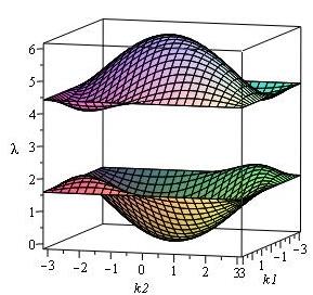
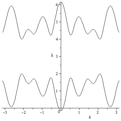
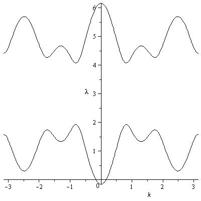
Figure 4. Left: the graphs of the band functions (the dispersion relation) of the Schrödinger operator $H_{{\bf G}}$ (when $q=1$) on the hexagonal lattice ${\bf G}$. Center and right: the graphs of the band functions of the Schrödinger operators $H_{{\bf G}_{\mathfrak{t}}}$ and $H_{{\bf G}_{\mathfrak{t}_{1}}}$ on the nanotubes ${\bf G}_{\mathfrak{t}}$ and ${\bf G}_{\mathfrak{t}_{1}}$ with the chiral vectors $\mathfrak{t}=5\mathfrak{a}_{1}+2\mathfrak{a}_{2}$ (center) and $\mathfrak{t}_{1}=2\mathfrak{a}_{1}+3\mathfrak{a}_{2}$ (right). The ranges of the corresponding band functions of $H_{{\bf G}}$ and $H_{{\bf G}_{\mathfrak{t}}}$ (left and center) coincide. The ranges of the corresponding band functions of $H_{{\bf G}}$ and $H_{{\bf G}_{\mathfrak{t}_{1}}}$ (left and right) are close to each other but do not coincide.

Isospectrality of periodic graphs in the sense of coinciding their spectra as sets does not imply Floquet and even Fermi isospectrality, since it only means that the ranges of the corresponding band functions are the same, but the band functions themselves may even depend on the quasimomenta of distinct dimensions. For example, the hexagonal lattice ${\bf G}$ and the nanotube ${\bf G}_{\mathfrak{t}}$ with a primitive chiral vector $\mathfrak{t}=t_{1}\mathfrak{a}_{1}+t_{2}\mathfrak{a}_{2}$, $t_{1}-t_{2}\in 3{\mathbb{Z}}$, are isospectral ($\mathfrak{a}_{1},\mathfrak{a}_{2}$ are the periods of the hexagonal lattice), see Example 2.8. The graphs of the band functions (the dispersion relations) of the Schrödinger operators $H_{\bf G}$ on ${\bf G}$ and $H_{{\bf G}_{\mathfrak{t}}}$ on ${\bf G}_{\mathfrak{t}}$ with $\mathfrak{t}=5\mathfrak{a}_{1}+2\mathfrak{a}_{2}$ are plotted in Fig. 4 (when $q=1$). The band functions of $H_{\bf G}$ (left) depend on the two-dimensional quasimomentum $k=(k_{1},k_{2})$. The band functions of $H_{{\bf G}_{\mathfrak{t}}}$ (center) are functions of the one-dimensional quasimomentum $k$. But the ranges of these band functions are the same.

Remark 2.14.

i) For each primitive set $\mathfrak{t}\subset\Gamma$ the periodic graph ${\mathcal{G}}$ and its subcovering ${\mathcal{G}}_{\mathfrak{t}}$ have the same periodic spectrum (i.e., they are also periodic isospectral). Indeed, the Floquet operators $H(0)$ and $H_{\mathfrak{t}}(0)$ are the Schrödinger operators with the same potential $Q$ on the same fundamental graph ${\mathcal{G}}_{*}$ of ${\mathcal{G}}$ and ${\mathcal{G}}_{\mathfrak{t}}$ (see Remark 1.2 and the identity (2.1)).

ii) Notion of asymptotic isospectrality for Schrödinger operators on periodic graphs was introduced in [S24] when studying the behavior of the spectrum of the Schrödinger operators on periodic graphs under perturbations of graphs by adding edges (between existing vertices) in a periodic way.

3. Proof of the main results

3.1. A particular choice of the Brillouin zone.

Let ${\mathcal{G}}\subset{\mathbb{R}}^{d}$ be a $\Gamma$-periodic graph, where $\Gamma\subset{\mathbb{R}}^{d}$ is the lattice with the basis $\{\mathfrak{a}_{1},\ldots,\mathfrak{a}_{d}\}$. Recall that the band functions $\lambda_{j}(k)$ of the Schrödinger operator $H$ on ${\mathcal{G}}$ are $2\pi{\mathbb{Z}}^{d}$-periodic in $k\in{\mathbb{R}}^{d}$. In order to prove our main results we need a particular choice of the Brillouin zone for ${\mathcal{G}}$ instead of ${\mathcal{B}}=(-\pi,\pi]^{d}$. By a Brillouin zone we understand any choice of the fundamental domain of the lattice $2\pi{\mathbb{Z}}^{d}$ in the momentum space.

Let ${\mathcal{G}}_{\mathfrak{t}}$ be a subcovering of ${\mathcal{G}}$ with a primitive set $\mathfrak{t}=\{\mathfrak{t}_{1},\ldots,\mathfrak{t}_{d_{o}}\}$, $d_{o}<d$, of the lattice $\Gamma$. This primitive set $\mathfrak{t}$ can be extended to a basis

$$\{\mathfrak{t}_{1},\ldots,\mathfrak{t}_{d_{o}},\mathfrak{t}_{d_{o}+1},\ldots,\mathfrak{t}_{d}\}$$ (3.1)

of $\Gamma$. The two bases of the same lattice $\Gamma$ are related by the $d\times d$ unimodular matrix $\widetilde{\mathcal{T}}$ (i.e., the integer matrix with the determinant $\pm 1$) given by

$$\widetilde{\mathcal{T}}=(t_{ij})_{i,j=1}^{d},\quad\textrm{where}\quad\mathfrak{t}_{i}=\sum\limits_{j=1}^{d}t_{ij}\mathfrak{a}_{j},\qquad t_{ij}\in{\mathbb{Z}},\qquad\mathop{\mathrm{det}}\nolimits\widetilde{\mathcal{T}}=\pm 1.$$ (3.2)

The rows of $\widetilde{\mathcal{T}}$ are the coordinates of $\mathfrak{t}_{s}\in\Gamma$, $s\in{\mathbb{N}}_{d}$, with respect to the basis $\{\mathfrak{a}_{1},\ldots,\mathfrak{a}_{d}\}$. Note that the first $d_{o}$ rows of $\widetilde{\mathcal{T}}$ form the chiral matrix ${\mathcal{T}}$ of the subcovering ${\mathcal{G}}_{\mathfrak{t}}$, see (1.8), (1.9). This change of the basis of the lattice $\Gamma$ determines the linear change in the quasimomentum $k$:

$$\kappa=\widetilde{\mathcal{T}}k,\qquad k\in{\mathbb{R}}^{d},$$

and the new Brillouin zone $\widetilde{\mathcal{B}}$ for ${\mathcal{G}}$ given by

$$\widetilde{\mathcal{B}}=\big{\{}k\in{\mathbb{R}}^{d}:\widetilde{\mathcal{T}}k\in(-\pi,\pi]^{d}\big{\}}.$$ (3.3)

To describe the spectrum of the Schrödinger operator $H_{\mathfrak{t}}$ on the subcovering ${\mathcal{G}}_{\mathfrak{t}}$ of the periodic graph ${\mathcal{G}}$ we need to define the ranges of the band functions $\lambda_{j}(k)$ of the Schrödinger operator $H$ on ${\mathcal{G}}$ restricted to the set ${\mathcal{B}}_{\mathfrak{t}}$ given by

$${\mathcal{B}}_{\mathfrak{t}}=\big{\{}k\in(-\pi,\pi]^{d}:{\mathcal{T}}k\in 2\pi{\mathbb{Z}}^{d_{o}}\big{\}},$$ (3.4)

where ${\mathcal{T}}$ is the chiral matrix of the subcovering ${\mathcal{G}}_{\mathfrak{t}}$, see Section 1.3.

Lemma 3.1.

The ranges of the band functions $\lambda_{j}(k)$ of the Schrödinger operator $H$ on the periodic graph ${\mathcal{G}}$, restricted to the set ${\mathcal{B}}_{\mathfrak{t}}$ defined by (3.4), have the form

$$\begin{array}[]{l}\displaystyle\lambda_{j}({\mathcal{B}}_{\mathfrak{t}})=\lambda_{j}(\widetilde{\mathcal{B}}_{\mathfrak{t}})=\big{[}\lambda_{j}^{-}(\mathfrak{t}),\lambda_{j}^{+}(\mathfrak{t})\big{]},\qquad j\in{\mathbb{N}}_{\nu},\qquad\textrm{where}\\[6.0pt] \displaystyle\lambda_{j}^{-}(\mathfrak{t})=\min_{k\in\widetilde{\mathcal{B}}_{\mathfrak{t}}}\lambda_{j}(k)=\min_{k\in{\mathcal{B}}_{\mathfrak{t}}}\lambda_{j}(k),\qquad\lambda_{j}^{+}(\mathfrak{t})=\max_{k\in\widetilde{\mathcal{B}}_{\mathfrak{t}}}\lambda_{j}(k)=\max_{k\in{\mathcal{B}}_{\mathfrak{t}}}\lambda_{j}(k),\end{array}$$ (3.5)

and the subset $\widetilde{\mathcal{B}}_{\mathfrak{t}}$ of the new Brillouin zone $\widetilde{\mathcal{B}}$, see (3.3), is given by

$$\widetilde{\mathcal{B}}_{\mathfrak{t}}=\big{\{}k\in\widetilde{\mathcal{B}}:{\mathcal{T}}k=0\big{\}}.$$ (3.6)

Proof. The band functions $\lambda_{j}(k)$ are $2\pi{\mathbb{Z}}^{d}$-periodic in $k\in{\mathbb{R}}^{d}$. Taking into account that the set ${\mathcal{S}}_{\mathfrak{t}}:=\{k\in{\mathbb{R}}^{d}:{\mathcal{T}}k\in 2\pi{\mathbb{Z}}^{d_{o}}\}$ is $2\pi{\mathbb{Z}}^{d}$-invariant, we obtain

$$\lambda_{j}({\mathcal{B}}_{\mathfrak{t}})=\lambda_{j}({\mathcal{S}}_{\mathfrak{t}})=\lambda_{j}({\mathcal{S}}_{\mathfrak{t}}\cap\widetilde{\mathcal{B}})=\lambda_{j}(\widetilde{\mathcal{B}}_{\mathfrak{t}}).$$

The set $\widetilde{\mathcal{B}}_{\mathfrak{t}}$ is connected, since its image under the linear isomorphism $\widetilde{\mathcal{T}}$ defined by (3.2) is the connected set $\{0\}^{d_{o}}\times(-\pi,\pi]^{d-d_{o}}$. Then, using that $\lambda_{j}(k)$ are continuous, we get

$$\lambda_{j}(\widetilde{\mathcal{B}}_{\mathfrak{t}})=\big{[}\lambda_{j}^{-}(\mathfrak{t}),\lambda_{j}^{+}(\mathfrak{t})\big{]},\qquad j\in{\mathbb{N}}_{\nu},$$

where $\lambda_{j}^{\pm}(\mathfrak{t})$ are given in (3.5). $\Box$

The following example illustrates Lemma 3.1.

Figure 5. Two choices of the Brillouin zone in terms of the quasimomenta $k=(k_{1},k_{2})\in(-\pi,\pi]^{2}$ (the square ${\mathcal{B}}$ bounded by dashed lines) and $\kappa=\widetilde{\mathcal{T}}k$, $\kappa=(\kappa_{1},\kappa_{2})\in(-\pi,\pi]^{2}$ (the shaded parallelogram $\widetilde{\mathcal{B}}$). The lines $L_{n}$ (marked in red color) are given by the equations $t_{1}k_{1}+t_{2}k_{2}=2\pi n$, $n\in{\mathbb{Z}}$, when $(t_{1},t_{2})=(2,3)$. The lines $L_{0},L_{\pm 1},L_{\pm 2}$ intersect the square Brillouin zone ${\mathcal{B}}$. The line $L_{0}$ (which coincides with the axis $\kappa_{2}$) is the single line among $L_{n}$ that enters the shaded Brillouin zone $\widetilde{\mathcal{B}}$.

Example 3.2.

We consider the hexagonal lattice ${\bf G}$, which is a $\Gamma$-periodic graph, where $\Gamma\subset{\mathbb{R}}^{2}$ is the lattice with the basis $\{\mathfrak{a}_{1},\mathfrak{a}_{2}\}$, see Fig. 1a. Let ${\bf G}_{\mathfrak{t}_{1}}$ be the subcovering of ${\bf G}$ (the nanotube) with the primitive chiral vector $\mathfrak{t}_{1}=2\mathfrak{a}_{1}+3\mathfrak{a}_{2}$. The primitive vector $\mathfrak{t}_{1}$ can be completed to the basis $\{\mathfrak{t}_{1},\mathfrak{t}_{2}\}$ of $\Gamma$ by the vector $\mathfrak{t}_{2}=\mathfrak{a}_{1}+2\mathfrak{a}_{2}$. Thus, the matrix $\widetilde{\mathcal{T}}$ defined by (3.2) has the form

$$\widetilde{\mathcal{T}}=\left(\begin{array}[]{cc}2&3\\ 1&2\end{array}\right),\qquad\mathop{\mathrm{det}}\nolimits\widetilde{\mathcal{T}}=1.$$

In Fig. 5 we show two choices of the Brillouin zone for the hexagonal lattice ${\bf G}$:
$\bullet$ the square ${\mathcal{B}}$ (bounded by dashed lines) drawn in terms of the quasimomentum $k=(k_{1},k_{2})\in(-\pi,\pi]^{2}$, and
$\bullet$ the parallelogram $\widetilde{\mathcal{B}}$ (shaded in the figure) drawn in terms of the quasimomentum $\kappa=\widetilde{\mathcal{T}}k$, $\kappa=(\kappa_{1},\kappa_{2})\in(-\pi,\pi]^{2}$.
The lines $L_{n}$ shown in the figure are given by the equations $t_{1}k_{1}+t_{2}k_{2}=2\pi n$, $n\in{\mathbb{Z}}$, where $(t_{1},t_{2})=(2,3)$ is the chiral index of the nanotube ${\bf G}_{\mathfrak{t}_{1}}$. The set ${\mathcal{B}}_{\mathfrak{t}_{1}}$ defined by (3.4) consists of the five segments of the lines $L_{0},L_{\pm 1},L_{\pm 2}$ inside the square Brillouin zone ${\mathcal{B}}$. The set $\widetilde{\mathcal{B}}_{\mathfrak{t}_{1}}$ defined by (3.6) consists of only the part of the line $L_{0}$ inside the Brillouin zone $\widetilde{\mathcal{B}}$. The line $L_{0}$ coincides with the axis $\kappa_{2}$.

The dispersion relation for the Schrödinger operator $H_{\bf G}=\Delta_{\bf G}+Q$ on ${\bf G}$ with a $\Gamma$-periodic potential $Q$ defined by (2.8) is plotted in Fig. 4 (left), when $q=1$. The Brillouin zone is parameterized by the quasimomentum $k$. The band functions of the Schrödinger operator $H_{{\bf G}_{\mathfrak{t}_{1}}}$ on the nanotube ${\bf G}_{\mathfrak{t}_{1}}$ are the restrictions of the dispersion relation for $H_{\bf G}$ to the segment of the line $L_{0}$ given by the equation $2k_{1}+3k_{2}=0$ (or, $\kappa_{1}=0$, in terms of $\kappa$) inside the Brillouin zone $\widetilde{\mathcal{B}}$, see Fig. 4 (right).

Remark 3.3.

In fact, the set $\widetilde{\mathcal{B}}_{\mathfrak{t}}$ given by (3.6) is a natural choice of the Brillouin zone for the subcovering ${\mathcal{G}}_{\mathfrak{t}}$ which is a $\Gamma_{o}$-periodic graph, where $\Gamma_{o}$ is the sublattice of $\Gamma$ of rank $d-d_{o}$ with the basis $\{\mathfrak{t}_{d_{o}+1},\ldots,\mathfrak{t}_{d}\}$, see (3.1).

3.2. Asymptotically isospectral graphs.

In the proofs of our main results we will use the following known statement, see, e.g., p.421 in [HJ85].

Proposition 3.4.

For a system of linear equations $Ay=b$, where $A$ is a real $m\times n$ matrix and $b\in{\mathbb{R}}^{m}$, $y\in{\mathbb{R}}^{n}$, the solution $\hat{y}$ of minimum Euclidean norm $|\hat{y}|$ is given by

$$\hat{y}=A^{+}b,$$

where $A^{+}$ is the Moore-Penrose pseudo-inverse of a matrix $A$. If the matrix $A$ has full row rank (i.e., $AA^{\top}$ is invertible), then

$$A^{+}=A^{\top}(AA^{\top})^{-1},$$

where $A^{\top}$ is the transpose of $A$, and

$$|\hat{y}|=|A^{+}b|=\big{|}(AA^{\top})^{-1/2}b\big{|}.$$

We prove Propositions 2.2 and 2.4 about asymptotic isospectrality and just isospectrality of periodic graphs and their subcoverings.

Proof of Proposition 2.2. Due to (1.11), the spectrum of the Schrödinger operator $H_{\mathfrak{t}}$ on the subcovering ${\mathcal{G}}_{\mathfrak{t}}$ is given by

$$\sigma(H_{\mathfrak{t}})=\bigcup_{k\in{\mathcal{B}}_{\mathfrak{t}}}\sigma\big{(}H(k)\big{)}=\bigcup_{k\in{\mathcal{B}}_{\mathfrak{t}}}\bigcup_{j=1}^{\nu}\lambda_{j}(k)=\bigcup_{j=1}^{\nu}\lambda_{j}({\mathcal{B}}_{\mathfrak{t}}),$$ (3.7)

where $\lambda_{j}(k)$ are the band functions of the Schrödinger operator $H$ on the periodic graph ${\mathcal{G}}$, and the set ${\mathcal{B}}_{\mathfrak{t}}\subset{\mathcal{B}}:=(-\pi,\pi]^{d}$ is defined by (1.10). Combining (3.7) and (3.5), we obtain that the spectrum of $H_{\mathfrak{t}}$ has the form (2.2), where the last two inequalities follow from the inclusion ${\mathcal{B}}_{\mathfrak{t}}\subset{\mathcal{B}}$.

Now we prove the identities (2.3). Let $j\in{\mathbb{N}}_{\nu}$. We prove (2.3) for $\lambda_{j}^{-}(\mathfrak{t})$. The proof for $\lambda_{j}^{+}(\mathfrak{t})$ is similar. Due to $2\pi{\mathbb{Z}}^{d}$-periodicity of the band function $\lambda_{j}(k)$, we have

$$\lambda_{j}^{-}:=\min_{k\in{\mathcal{B}}}\lambda_{j}(k)=\min_{k\in{\mathbb{R}}^{d}}\lambda_{j}(k)=\lambda_{j}(k_{o})$$

for some $k_{o}\in\widetilde{\mathcal{B}}$, where the new Brillouin zone $\widetilde{\mathcal{B}}$ is defined by (3.3). Let $\hat{k}$ be the point in the set

$$L_{0}=\{k\in{\mathbb{R}}^{d}:{\mathcal{T}}k=0\}$$

that is closest to the point $k_{o}$, i.e.,

$$\min\limits_{k\in L_{0}}|k-k_{o}|=|\hat{k}-k_{o}|.$$

Then $\hat{k}-k_{o}$ is the solution of the system of linear equations ${\mathcal{T}}(k-k_{o})=-{\mathcal{T}}k_{o}$ with minimum Euclidean norm $|\hat{k}-k_{o}|$. Due to Proposition 3.4, this solution has the form

$$\hat{k}-k_{o}=-{\mathcal{T}}^{+}\,{\bf x}_{o},\qquad\textrm{where}\qquad{\bf x}_{o}={\mathcal{T}}k_{o},$$

and

$$|\hat{k}-k_{o}|=\big{|}({\mathcal{T}}{\mathcal{T}}^{\top})^{-1/2}{\bf x}_{o}\big{|}.$$ (3.8)

Since $k_{o}\in\widetilde{\mathcal{B}}$, we get ${\bf x}_{o}={\mathcal{T}}k_{o}\in(-\pi,\pi]^{d_{o}}$, see (3.3). Then from (3.8) we obtain

$$\textstyle|\hat{k}-k_{o}|\leqslant\frac{\pi\sqrt{d_{o}}}{\tau}=O\big{(}\frac{1}{\tau}\big{)},$$ (3.9)

where $\tau$ is the smallest eigenvalue of $({\mathcal{T}}{\mathcal{T}}^{\top})^{1/2}$. Using the first inequality in (2.2) and $2\pi{\mathbb{Z}}^{d}$-periodicity of the band function $\lambda_{j}(k)$, we have

$$\lambda_{j}^{-}\leqslant\lambda_{j}^{-}(\mathfrak{t})=\min_{k\in{\mathcal{B}}_{\mathfrak{t}}}\lambda_{j}(k)=\min_{k\in{\mathcal{S}}_{\mathfrak{t}}}\lambda_{j}(k)\leqslant\lambda_{j}(\hat{k}),$$

since $\hat{k}\in L_{0}\subset{\mathcal{S}}_{\mathfrak{t}}:=\{k\in{\mathbb{R}}^{d}:{\mathcal{T}}k\in 2\pi{\mathbb{Z}}^{d_{o}}\}$. This, (3.9) and continuity of the band function $\lambda_{j}(\cdot)$ yield

$$\lambda_{j}^{-}\leqslant\lim_{\tau\to\infty}\lambda_{j}^{-}(\mathfrak{t})\leqslant\lim_{\tau\to\infty}\lambda_{j}(\hat{k})=\lambda_{j}(k_{o})=\lambda_{j}^{-}.$$

Thus, $\lim\limits_{\tau\to\infty}\lambda_{j}^{-}(\mathfrak{t})=\lambda_{j}^{-}$.  $\Box$

Proof of Proposition 2.4. We prove this proposition for the band edge $\lambda_{j}^{-}(\mathfrak{t})$. The proof for $\lambda_{j}^{+}(\mathfrak{t})$ is similar. Let the condition (2.5) be fulfilled for some $k_{o}\in K_{j}^{-}$. Then $k_{o}\in{\mathcal{B}}_{\mathfrak{t}}$ (see (1.10)) and,

$$\lambda_{j}^{-}(\mathfrak{t})=\min_{k\in{\mathcal{B}}_{\mathfrak{t}}}\lambda_{j}(k)\leqslant\lambda_{j}(k_{o})=\lambda_{j}^{-}.$$

This and the first inequality in (2.2) yield $\lambda_{j}^{-}(\mathfrak{t})=\lambda_{j}^{-}$.

Conversely, let $\lambda_{j}^{-}(\mathfrak{t})=\lambda_{j}^{-}$. Then for some $k_{o}\in{\mathcal{B}}_{\mathfrak{t}}$ we have

$$\lambda_{j}^{-}(\mathfrak{t})=\min_{k\in{\mathcal{B}}_{\mathfrak{t}}}\lambda_{j}(k)=\lambda_{j}(k_{o})=\lambda_{j}^{-}.$$

Thus, $k_{o}\in K_{j}^{-}$ and $k_{o}$ satisfies the condition (2.5) (since $k_{o}\in{\mathcal{B}}_{\mathfrak{t}}$).

i) Let $0\in K_{j}^{-}$. For $k_{o}=0$ the condition (2.5) holds. Then $\lambda_{j}^{-}(\mathfrak{t})=\lambda_{j}^{-}$.

ii) Let $k_{o}:=(\pi,\ldots,\pi)\in K_{j}^{-}$ and the sum of the entries in each row of ${\mathcal{T}}$ be even. Then the condition (2.5) holds, and $\lambda_{j}^{-}(\mathfrak{t})=\lambda_{j}^{-}$.  $\Box$

3.3. Asymptotics of the band edges.

We prove Theorem 2.6 about asymptotics of the band edges $\lambda_{j}^{\pm}(\mathfrak{t})$ of the Schrödinger operator $H_{\mathfrak{t}}$ on the subcovering ${\mathcal{G}}_{\mathfrak{t}}$ as all chiral vectors from the primitive set $\mathfrak{t}$ are long enough.

Proof of Theorem 2.6. We prove (2.6) for $\lambda_{j}^{-}(\mathfrak{t})$. The proof for $\lambda_{j}^{+}(\mathfrak{t})$ is similar. Due to (3.5) and $2\pi{\mathbb{Z}}^{d}$-periodicity of the band function $\lambda_{j}(k)$, we have

$$\lambda_{j}^{-}(\mathfrak{t})=\min_{k\in\widetilde{\mathcal{B}}_{\mathfrak{t}}}\lambda_{j}(k)=\min_{k\in L_{0}}\lambda_{j}(k),$$ (3.10)

where $\widetilde{\mathcal{B}}_{\mathfrak{t}}$ is given by (3.6) and $L_{0}=\big{\{}k\in{\mathbb{R}}^{d}:{\mathcal{T}}k=0\big{\}}$. Thus, in order to get the band edge $\lambda^{-}_{j}(\mathfrak{t})$ we need to find the minimum of $\lambda_{j}(k)$ with the constraint ${\mathcal{T}}k=0$, where ${\mathcal{T}}$ is the chiral matrix of the subcovering ${\mathcal{G}}_{\mathfrak{t}}$ defined by by (1.8), (1.9).

Let $\tilde{k}_{o}$ be the point from the new Brillouin zone $\widetilde{\mathcal{B}}$, see (3.3), such that $\tilde{k}_{o}\equiv k_{o}\,(\mod 2\pi{\mathbb{Z}}^{d})$. Due to $2\pi{\mathbb{Z}}^{d}$-periodicity, the function $\lambda_{j}(k)$ has the non-degenerate minimum $\lambda_{j}^{-}$ at the point $\tilde{k}_{o}$ and also satisfies the assumption A at this point $\tilde{k}_{o}\in\widetilde{\mathcal{B}}$. The Taylor expansion of the function $\lambda_{j}(k)$ about the point $\tilde{k}_{o}$ is given by

$$\begin{array}[]{l}\textstyle\lambda_{j}(k)=\lambda_{j}^{-}+\frac{1}{2}\langle k-\tilde{k}_{o},{\bf H}(k-\tilde{k}_{o})\rangle+g_{1}(k-\tilde{k}_{o}),\qquad\textrm{where}\\[6.0pt] {\bf H}=\mathrm{Hess}\,\lambda_{j}(\tilde{k}_{o})=\mathrm{Hess}\,\lambda_{j}(k_{o}),\\[6.0pt] \lambda_{j}^{-}=\lambda_{j}(\tilde{k}_{o})=\lambda_{j}(k_{o}),\qquad g_{1}(k-\tilde{k}_{o})=O\big{(}|k-\tilde{k}_{o}|^{3}\big{)}.\end{array}$$ (3.11)

We make the non-degenerate change of variables $k\mapsto y$, where

$$y={\bf H}^{1/2}(k-\tilde{k}_{o}),$$

and ${\bf H}^{1/2}$ is the positive definite square root of the positive definite Hessian ${\bf H}$. In the new variable $y$ the expansion (3.11) and the constraint ${\mathcal{T}}k=0$ have the form

$$\textstyle\lambda_{j}\big{(}k(y)\big{)}=\lambda_{j}^{-}+\frac{1}{2}|y|^{2}+g_{2}(y),\qquad g_{2}(y)=g_{1}({\bf H}^{-1/2}y)=O\big{(}|y|^{3}\big{)},$$ (3.12)

$$\textstyle{\mathcal{T}}({\bf H}^{-1/2}y+\tilde{k}_{o})=0.$$ (3.13)

Among all solutions of the system (3.13) we need to find the solution $\hat{y}$ with minimum Euclidean norm $|\hat{y}|$. The $d_{o}\times d$ matrix ${\mathcal{T}}{\bf H}^{-1/2}$ has full row rank. Thus, due to Proposition 3.4, the solution $\hat{y}$ of the system of the linear equations (3.13) with minimum $|\hat{y}|$ has the form

$$\hat{y}=-({\mathcal{T}}{\bf H}^{-1/2})^{+}\,{\bf x}_{o},\qquad{\bf x}_{o}={\mathcal{T}}\tilde{k}_{o},$$

and

$$|\hat{y}|^{2}=\big{|}\big{(}{\mathcal{T}}{\bf H}^{-1/2}({\mathcal{T}}{\bf H}^{-1/2})^{\top}\big{)}^{-1/2}{\bf x}_{o}\big{|}^{2}=\big{|}({\mathcal{T}}{\bf H}^{-1}{\mathcal{T}}^{\top})^{-1/2}{\bf x}_{o}\big{|}^{2}.$$ (3.14)

We note that

$\bullet$ ${\mathcal{T}}\tilde{k}_{o}\in(-\pi,\pi]^{d_{o}}$, since $\tilde{k}_{o}\in\widetilde{\mathcal{B}}$ (see (3.3)), and

$\bullet$ ${\mathcal{T}}\tilde{k}_{o}\equiv{\mathcal{T}}k_{o}\,(\mod 2\pi{\mathbb{Z}}^{d_{o}})$, since $\tilde{k}_{o}\equiv k_{o}\,(\mod 2\pi{\mathbb{Z}}^{d})$ and ${\mathcal{T}}$ is a $d_{o}\times d$ integer matrix.

The identity (3.14) yields

$$|\hat{y}|^{2}\leqslant\lambda_{\max}\big{(}({\mathcal{T}}{\bf H}^{-1}{\mathcal{T}}^{\top})^{-1}\big{)}\cdot|{\bf x}_{o}|^{2}=\frac{|{\bf x}_{o}|^{2}}{\lambda_{\min}({\mathcal{T}}{\bf H}^{-1}{\mathcal{T}}^{\top})}\,,$$ (3.15)

where $\lambda_{\min}(A)$ and $\lambda_{\max}(A)$ denote, respectively, the smallest and largest eigenvalues of a self-adjoint matrix $A$. Let $\phi\in{\mathbb{R}}^{d_{o}}$ be the unit-norm eigenvector of ${\mathcal{T}}{\bf H}^{-1}{\mathcal{T}}^{\top}$ corresponding to $\lambda_{\min}({\mathcal{T}}{\bf H}^{-1}{\mathcal{T}}^{\top})$. Then

$$\lambda_{\min}({\mathcal{T}}{\bf H}^{-1}{\mathcal{T}}^{\top})=\langle\phi,{\mathcal{T}}{\bf H}^{-1}{\mathcal{T}}^{\top}\phi\rangle=\langle{\mathcal{T}}^{\top}\phi,{\bf H}^{-1}{\mathcal{T}}^{\top}\phi\rangle\geqslant\lambda_{\min}({\bf H}^{-1})\langle{\mathcal{T}}^{\top}\phi,{\mathcal{T}}^{\top}\phi\rangle\\ =\lambda_{\min}({\bf H}^{-1})\langle\phi,{\mathcal{T}}{\mathcal{T}}^{\top}\phi\rangle\geqslant\lambda_{\min}({\bf H}^{-1})\lambda_{\min}({\mathcal{T}}{\mathcal{T}}^{\top}).$$ (3.16)

Substituting (3.16) into (3.15) and using that $\tau^{2}=\lambda_{\min}({\mathcal{T}}{\mathcal{T}}^{\top})$ and ${\bf x}_{o}\in(-\pi,\pi]^{d_{o}}$, we obtain

$$|\hat{y}|^{2}\leqslant\frac{\pi^{2}d_{o}}{\lambda_{\min}({\bf H}^{-1})\,\tau^{2}}=\frac{\pi^{2}d_{o}}{\tau^{2}}\,\lambda_{\max}({\bf H}),$$

which yields

$$|\hat{y}|=\textstyle O(\frac{1}{\tau}).$$ (3.17)

Using (3.10), (3.12) and (3.14) we get

$$\textstyle\lambda_{j}^{-}(\mathfrak{t})=\lambda_{j}(k(\hat{y}))=\lambda_{j}^{-}+\frac{1}{2}\,|\hat{y}|^{2}+g_{2}(\hat{y})=\lambda_{j}^{-}+\frac{1}{2}\,\big{|}({\mathcal{T}}{\bf H}^{-1}{\mathcal{T}}^{\top})^{-1/2}{\bf x}_{o}\big{|}^{2}+g_{2}(\hat{y}),$$

where $g_{2}(\hat{y})=O(|\hat{y}|^{3})$, or, using (3.17), $g_{2}(\hat{y})=O(\frac{1}{\tau^{3}})$. Thus, (2.6) is proved.

If all components of $k_{o}$ are equal to either 0 or $\pi$, then $\tilde{k}_{o}\in\pi{\mathbb{Z}}^{d}$, and, due to $2\pi{\mathbb{Z}}^{d}$-periodicity and evenness of $\lambda_{j}$, we have

$$\lambda_{j}(k+\tilde{k}_{o})=\lambda_{j}(-k-\tilde{k}_{o})=\lambda_{j}(-k+\tilde{k}_{o}),$$

since $2\tilde{k}_{o}\in 2\pi{\mathbb{Z}}^{d}$. This implies that the Taylor series (3.11) of $\lambda_{j}$ at $\tilde{k}_{o}$ has only even degree terms. Then, $g_{1}(k-\tilde{k}_{o})=O\big{(}|k-\tilde{k}_{o}|^{4}\big{)}$ and $g_{2}(\hat{y})=O(\frac{1}{\tau^{4}})$.

Finally, let $d_{o}=1$, i.e., the set $\mathfrak{t}$ consists of a single primitive vector with a chiral index $t\in{\mathbb{Z}}^{d}$. Then ${\mathcal{T}}=t^{\top}$,

$$\tau=(t^{\top}t)^{1/2}=|t|,\quad{\mathcal{T}}{\bf H}^{-1}{\mathcal{T}}^{\top}=t^{\top}{\bf H}^{-1}t=|{\bf H}^{-1/2}t|^{2},\quad{\bf x}_{o}=(\langle t,k_{o}\rangle\mod 2\pi)\in(-\pi,\pi],$$

and, the asymptotics (2.6) has the form (2.7).  $\Box$

4. Examples

In this section we consider simple examples of periodic graphs and describe the spectrum of the Schrödinger operators on their subcoverings.

4.1. Nanotubes

The hexagonal lattice ${\bf G}$ is a $\Gamma$-periodic graph, where $\Gamma\subset{\mathbb{R}}^{2}$ is the lattice with the basis $\mathfrak{a}_{1},\mathfrak{a}_{2}$, see Fig. 1a. The fundamental graph ${\bf G}_{*}$ of ${\bf G}$ consists of two vertices $v_{1},v_{2}$ and three multiple edges connecting these vertices, see Fig. 1d. First we describe the spectrum of the Schrödinger operator $H=\Delta+Q$ on ${\bf G}$ with a $\Gamma$-periodic potential $Q$.

Lemma 4.1.

The spectrum of the Schrödinger operator $H=\Delta+Q$ on the hexagonal lattice ${\bf G}$ with the potential $Q$ defined by (2.8) is given by

$$\sigma(H)=[\lambda_{1}^{-},\lambda_{1}^{+}]\cup[\lambda_{2}^{-},\lambda_{2}^{+}],$$ (4.1)

$$\begin{array}[]{ll}\lambda_{1}^{-}=\lambda_{1}(K_{1}^{-})=3-\sqrt{9+q^{2}},&\lambda_{1}^{+}=\lambda_{1}(K_{1}^{+})=3-q,\\[6.0pt] \lambda_{2}^{-}=\lambda_{2}(K_{2}^{-})=3+q,&\lambda_{2}^{+}=\lambda_{2}(K_{2}^{+})=3+\sqrt{9+q^{2}},\end{array}$$

where the level sets

$$\textstyle K_{1}^{-}=K_{2}^{+}=\big{\{}(0,0)\big{\}},\qquad K_{1}^{+}=K_{2}^{-}=\big{\{}\big{(}\pm\frac{2\pi}{3}\,,\mp\frac{2\pi}{3}\big{)}\big{\}}.$$ (4.2)

Proof. For the hexagonal lattice ${\bf G}$, the Floquet operator $H(k)$ defined by (1.4) in the standard basis of $\ell^{2}(\{v_{1},v_{2}\})\cong{\mathbb{C}}^{2}$ has the following matrix:

$$H(k)=\left(\begin{array}[]{cc}3+q&-1-e^{ik_{1}}-e^{ik_{2}}\\ -1-e^{-ik_{1}}-e^{-ik_{2}}&3-q\end{array}\right),\qquad k=(k_{1},k_{2})\in{\mathcal{B}}=(-\pi,\pi]^{2}.$$

The eigenvalues of $H(k)$ are given by

$$\lambda_{j}(k)=3+(-1)^{j}\sqrt{f(k)+q^{2}},\quad j=1,2,\quad\textrm{where}$$ (4.3)

$$f(k)=|1+e^{ik_{1}}+e^{ik_{2}}|^{2}=3+2\cos k_{1}+2\cos k_{2}+2\cos(k_{1}-k_{2}).$$

We have

$$\textstyle\min\limits_{k\in{\mathcal{B}}}f(k)=f\big{(}\pm\frac{2\pi}{3}\,,\mp\frac{2\pi}{3}\big{)}=0,\qquad\max\limits_{k\in{\mathcal{B}}}f(k)=f(0,0)=9.$$

Then, using the definition of the band edges $\lambda_{j}^{\pm}$ in (1.6), we obtain that the spectrum of $H$ has the form (4.1), (4.2).  $\Box$

Now we prove Example 2.8 about the spectrum of the Schrödinger operator $H_{\mathfrak{t}}=\Delta_{\mathfrak{t}}+Q$ on a nanotube ${\bf G}_{\mathfrak{t}}$ with a primitive chiral vector $\mathfrak{t}$.

Proof of Example 2.8. Due to Proposition 2.2, the spectrum of the Schrödinger operator $H_{\mathfrak{t}}$ on the nanotube ${\bf G}_{\mathfrak{t}}$ with a primitive chiral vector $\mathfrak{t}=t_{1}\mathfrak{a}_{1}+t_{2}\mathfrak{a}_{2}$ consists of two bands:

$$\sigma(H_{\mathfrak{t}})=[\lambda_{1}^{-}(\mathfrak{t}),\lambda_{1}^{+}(\mathfrak{t})]\cup[\lambda_{2}^{-}(\mathfrak{t}),\lambda_{2}^{+}(\mathfrak{t})].$$

Since $(0,0)\in K_{1}^{-}=K_{2}^{+}$, where $K_{j}^{\pm}$ are the level sets corresponding to the band edges $\lambda_{j}^{\pm}$ of the Schrödinger operator $H$ on the hexagonal lattice ${\bf G}$, see (4.1), (4.2), Proposition 2.4.i yields

$$\lambda_{1}^{-}(\mathfrak{t})=\lambda_{1}^{-}=3-\sqrt{9+q^{2}},\qquad\lambda_{2}^{+}(\mathfrak{t})=\lambda_{2}^{+}=3+\sqrt{9+q^{2}}.$$

i) Let $t_{1}-t_{2}\in 3{\mathbb{Z}}$. Then for the points $k_{o}=\big{(}\pm\frac{2\pi}{3}\,,\mp\frac{2\pi}{3}\big{)}\in K_{1}^{+}=K_{2}^{-}$ the condition (2.5) is fulfilled. Thus, due to Proposition 2.4 and the identities (4.1),

$$\textstyle\lambda_{1}^{+}(\mathfrak{t})=\lambda_{1}^{+}=3-q,\qquad\lambda_{2}^{-}(\mathfrak{t})=\lambda_{2}^{-}=3+q,$$

and $\varepsilon(\mathfrak{t})=0$ in (2.9).

ii) Let $t_{1}-t_{2}\not\in 3{\mathbb{Z}}$, i.e., $t_{1}-t_{2}=3m\pm 1$ for some $m\in{\mathbb{Z}}$. We obtain the asymptotics of the band edge $\lambda_{1}^{+}(\mathfrak{t})$ as $|t|\to\infty$, where $t=(t_{1},t_{2})$. The proof for $\lambda_{2}^{-}(\mathfrak{t})$ is similar. The point $k_{o}=\big{(}\frac{2\pi}{3}\,,-\frac{2\pi}{3}\big{)}$ is the only (up to evenness) maximum point of the band function $\lambda_{1}(k)$ in ${\mathcal{B}}=(-\pi,\pi]^{2}$, see (4.1), (4.2). Using the identity (4.3) for $\lambda_{1}(k)$, we obtain

$$\frac{\partial^{2}\lambda_{1}}{\partial k_{j}^{2}}\,(k_{o})=-\frac{1}{q}\,,\quad j=1,2;\qquad\frac{\partial^{2}\lambda_{1}}{\partial k_{1}\partial k_{2}}\,(k_{o})=\frac{1}{2q}\,.$$

Then the matrix ${\bf H}=-\mathrm{Hess}\,\lambda_{1}(k_{o})$ and its inverse are given by

$${\bf H}=\frac{1}{2q}\left(\begin{array}[]{rr}2&-1\\ -1&2\end{array}\right),\qquad{\bf H}^{-1}=\frac{2q}{3}\left(\begin{array}[]{cc}2&1\\ 1&2\end{array}\right).$$

Thus, the band function $\lambda_{1}(k)$ of $H$ satisfies the Assumption A and we can use the asymptotics (2.7). For $t=(t_{1},t_{2})$ and $k_{o}=\big{(}\frac{2\pi}{3}\,,-\frac{2\pi}{3}\big{)}$, we obtain

$$\textstyle|{\bf H}^{-1/2}t|^{2}=\langle t,{\bf H}^{-1}t\rangle=\frac{4q}{3}\,(t_{1}^{2}+t_{1}t_{2}+t_{2}^{2}),$$ (4.4)

$$\textstyle\langle t,k_{o}\rangle=\frac{2\pi}{3}\,(t_{1}-t_{2}).$$

Since $t_{1}-t_{2}=3m\pm 1$ for some $m\in{\mathbb{Z}}$,

$$\textstyle x_{o}:=(\langle t,k_{o}\rangle\mod 2\pi)=\pm\frac{2\pi}{3}\,.$$ (4.5)

Substituting (4.4), (4.5) and $\lambda_{1}^{+}=3-q$ into (2.7), we obtain

$$\textstyle\lambda_{1}^{+}(\mathfrak{t})=3-q-\frac{\pi^{2}}{6q(t_{1}^{2}+t_{1}t_{2}+t_{2}^{2})}+O\big{(}\frac{1}{|t|^{3}}\big{)}\qquad\textrm{as}\qquad|t|\to\infty.\qquad\Box$$

In the following example we consider a nanotube ${\bf G}_{\mathfrak{t}}$ with a non-primitive vector $\mathfrak{t}$.

Example 4.2.

Let ${\bf G}_{\mathfrak{t}}$ be the zig-zag nanotube with $\mathfrak{t}=2\mathfrak{a}_{1}$, see Fig. 1c. Then the spectrum $\sigma(H_{\mathfrak{t}})$ of the Schrödinger operator $H_{\mathfrak{t}}=\Delta_{\mathfrak{t}}+Q$ on ${\bf G}_{\mathfrak{t}}$ with the periodic potential $Q$ defined by (2.8) has the form

$$\begin{array}[]{l}\sigma(H_{\mathfrak{t}})=\sigma_{ac}(H_{\mathfrak{t}})\cup\sigma_{fb}(H_{\mathfrak{t}}),\qquad\sigma_{fb}(H_{\mathfrak{t}})=\{3\pm\sqrt{1+q^{2}}\,\},\\[8.0pt] \sigma_{ac}(H_{\mathfrak{t}})=\big{[}3-\sqrt{9+q^{2}}\,,3-\sqrt{1+q^{2}}\,\big{]}\cup\big{[}3+\sqrt{1+q^{2}}\,,3+\sqrt{9+q^{2}}\,\big{]}.\end{array}$$ (4.6)

Proof. The zigzag nanotube ${\bf G}_{\mathfrak{t}}$, $\mathfrak{t}=2\mathfrak{a}_{1}$, is a periodic graph with period $\mathfrak{a}_{2}$, see Fig. 1c. The fundamental graph $\widetilde{\bf G}_{*}=({\mathcal{V}}_{*},{\mathcal{E}}_{*})$ of ${\bf G}_{\mathfrak{t}}$ is shown in Fig. 1e, where ${\mathcal{V}}_{*}=\{v_{1},v_{2},v_{3},v_{4}\}$. For the nanotube ${\bf G}_{\mathfrak{t}}$, the matrix of the Floquet operator $H_{\mathfrak{t}}(k)$, $k\in(-\pi,\pi]$, defined by (1.4) in the standard basis of $\ell^{2}({\mathcal{V}}_{*})\cong{\mathbb{C}}^{4}$ has the form

$$H_{\mathfrak{t}}(k)=\left(\begin{array}[]{cc}A(k)&B\\ B&A(k)\end{array}\right),\quad A(k)=\left(\begin{array}[]{cc}3+q&-1-e^{ik}\\ -1-e^{-ik}&3-q\end{array}\right),\quad B=\left(\begin{array}[]{cc}0&-1\\ -1&0\end{array}\right).$$

The eigenvalues of $H_{\mathfrak{t}}(k)$ are given by

$$\lambda_{1,4}(k)=3\pm\sqrt{5+4\cos k+q^{2}}\,,\qquad\lambda_{2,3}=3\pm\sqrt{1+q^{2}}\,.$$

Then, using the definition of the band edges $\lambda_{j}^{\pm}$ in (1.6), we obtain that the spectrum of $H_{\mathfrak{t}}$ has the form (4.6).  $\Box$

Remark 4.3.

The spectra of the Schrödinger operators $H=\Delta+Q$ on the hexagonal lattice ${\bf G}$ and $H_{\mathfrak{t}}=\Delta_{\mathfrak{t}}+Q$ on any nanotube ${\bf G}_{\mathfrak{t}}$ with a primitive chiral vector $\mathfrak{t}$ (the periodic potential $Q$ is defined by (2.8)) consist of two spectral bands (see Example 2.8). The spectrum of the Schrödinger operator $H_{p\mathfrak{t}}=\Delta_{p\mathfrak{t}}+Q$ on a nanotube ${\bf G}_{p\mathfrak{t}}$ with the non-primitive chiral vector $p\mathfrak{t}$, where integer $p\geqslant 2$, has $2p$ bands. For example, the spectrum of $H_{2\mathfrak{a}_{1}}$ on the zigzag nanotube ${\bf G}_{2\mathfrak{a}_{1}}$ consists of four spectral bands, two of which are flat bands, see (4.6). But, due to (1.12), the inclusion $\sigma(H_{p\mathfrak{t}})\subseteq\sigma(H)$ still holds.

4.2. Subcoverings of the $d$-dimensional lattice

The $d$-dimensional lattice ${\mathbb{L}}^{d}$ is a ${\mathbb{Z}}^{d}$-periodic graph, for $d=3$ see Fig. 2a. The fundamental graph ${\mathbb{L}}^{d}_{*}$ of ${\mathbb{L}}^{d}$ consists of one vertex $v$ and $d$ loop edges at this vertex $v$ (Fig. 2d). The Floquet Laplacian $\Delta(k)$ for the lattice ${\mathbb{L}}^{d}$ has the form

$$\lambda_{1}(k)\equiv\Delta(k)=2d-2\cos k_{1}-\ldots-2\cos k_{d},\quad k=(k_{1},\ldots,k_{d})\in{\mathcal{B}}=(-\pi,\pi]^{d}.$$ (4.7)

Thus,

$$\textstyle\lambda_{1}^{-}=\min\limits_{k\in{\mathcal{B}}}\lambda_{1}(k)=\lambda_{1}(K_{1}^{-})=0,\qquad\lambda_{1}^{+}=\max\limits_{k\in{\mathcal{B}}}\lambda_{1}(k)=\lambda_{1}(K_{1}^{+})=4d,$$

where the level sets $K_{1}^{\pm}\subset{\mathcal{B}}$ consist of the single point:

$$K_{1}^{-}=\big{\{}(0,\ldots,0)\big{\}},\qquad K_{1}^{+}=\big{\{}\pi 1\!\!1_{d}\big{\}},\qquad 1\!\!1_{d}=(1,\ldots,1)\in{\mathbb{Z}}^{d}.$$

The spectrum of the Laplacian $\Delta$ on the $d$-dimensional lattice ${\mathbb{L}}^{d}$ is given by

$$\sigma(\Delta)=[\lambda_{1}^{-},\lambda_{1}^{+}]=[0,4d].$$

Now we prove Example 2.10 about the Laplacian spectrum on a subcovering ${\mathbb{L}}^{d}_{\mathfrak{t}}$ of the lattice ${\mathbb{L}}^{d}$ with a primitive set $\mathfrak{t}$ of chiral vectors $\mathfrak{t}_{1},\ldots,\mathfrak{t}_{d_{o}}$, where $\mathfrak{t}_{s}=(t_{s1},\ldots,t_{sd})\in{\mathbb{Z}}^{d}$, $s\in{\mathbb{N}}_{d_{o}}$, $d_{o}<d$.

Proof of Example 2.10. Due to Proposition 2.2, the spectrum of the Laplacian $\Delta_{\mathfrak{t}}$ on the subcovering ${\mathbb{L}}^{d}_{\mathfrak{t}}$ with a primitive set $\mathfrak{t}$ consists of the single band:

$$\sigma(\Delta_{\mathfrak{t}})=[\lambda_{1}^{-}(\mathfrak{t}),\lambda_{1}^{+}(\mathfrak{t})].$$

Since $0\in K_{1}^{-}$, then Proposition 2.4.i yields $\lambda_{1}^{-}(\mathfrak{t})=\lambda_{1}^{-}=0$. Thus, (2.10) is proved.

i) Let $\varrho_{s}:=t_{s1}+\ldots+t_{sd}$ be even for all $s\in{\mathbb{N}}_{d_{o}}$. Since $\pi 1\!\!1_{d}\in K_{1}^{+}$, due to Proposition 2.4.ii, we have $\lambda_{1}^{+}(\mathfrak{t})=\lambda_{1}^{+}=4d$.

ii) Let $\varrho_{s}$ be odd for some $s\in{\mathbb{N}}_{d_{o}}$. For the single maximum point $k_{o}=\pi 1\!\!1_{d}\in K_{1}^{+}$ of the single band function $\lambda_{1}(\cdot)$ of $\Delta$ given by (4.7) we obtain

$$\frac{\partial^{2}\lambda_{1}}{\partial k_{i}^{2}}\,(k_{o})=-2,\qquad\frac{\partial^{2}\lambda_{1}}{\partial k_{i}\partial k_{j}}\equiv 0,\qquad i,j\in{\mathbb{N}}_{d},\qquad i\neq j.$$

The matrix ${\bf H}=-\mathrm{Hess}\,\lambda_{1}(k_{o})$ and its inverse are given by

$$\textstyle{\bf H}=2I_{d},\qquad{\bf H}^{-1}=\frac{1}{2}\,I_{d},$$

where $I_{d}$ is the identity matrix of size $d$. Thus, the band function $\lambda_{1}(k)$ of $\Delta$ satisfies the Assumption A and we can use the asymptotics (2.6). Substituting

$$\textstyle\lambda_{1}^{+}=4d,\qquad k_{o}=\pi 1\!\!1_{d},\qquad{\bf H}^{-1}=\frac{1}{2}\,I_{d}$$

into (2.6), we obtain (2.11).

Finally, if $d_{o}=1$ and $\varrho_{1}$ is odd, then ${\mathcal{T}}=\mathfrak{t}_{1}^{\top}$, $\varrho=1$. Substituting this into (2.11), we obtain (2.12).  $\Box$

4.3. Subcoverings of the diamond lattice

We consider the diamond lattice ${\mathcal{G}}$ shown in Fig. 3a. The diamond lattice ${\mathcal{G}}$ is obtained by stacking together infinitely many copies

$${\bf G}+n\mathfrak{a}_{3}\subset{\mathbb{R}}^{3},\qquad\forall\,n\in{\mathbb{Z}},$$

of the hexagonal lattice ${\bf G}\subset{\mathbb{R}}^{2}$ along the vector $\mathfrak{a}_{3}=(0,0,1)$. Here ${\mathbb{R}}^{2}$ is considered as the subspace ${\mathbb{R}}^{2}\times\{0\}$ of ${\mathbb{R}}^{3}$. The copies of ${\bf G}$ are connected in a periodic way by the edges

$$\{v_{1},v_{2}+\mathfrak{a}_{3}\}+\mathfrak{a},\qquad\forall\,\mathfrak{a}\in\Gamma,$$

between the vertex $v_{1}+\mathfrak{a}$ in a lower copy and the vertex $v_{2}+\mathfrak{a}_{3}+\mathfrak{a}$ in the next copy, $\mathfrak{a}\in\Gamma$, where $v_{1},v_{2}$ are the vertices of ${\bf G}$ from the fundamental cell $\Omega$, and $\Gamma$ is the lattice with the basis $\mathfrak{a}_{1},\mathfrak{a}_{2},\mathfrak{a}_{3}$. The diamond lattice ${\mathcal{G}}$ is a $\Gamma$-periodic graph with the fundamental graph ${\mathcal{G}}_{*}$ consisting of two vertices $v_{1},v_{2}$ and four multiple edges connecting these vertices, see Fig. 3d.

First we describe the spectrum of the Schrödinger operator $H=\Delta+Q$ on the diamond lattice ${\mathcal{G}}$ with a $\Gamma$-periodic potential $Q$ defined by (2.13).

Lemma 4.4.

The spectrum of the Schrödinger operator $H=\Delta+Q$ on the diamond lattice ${\mathcal{G}}$ with the potential $Q$ defined by (2.13) is given by

$$\sigma(H)=[\lambda_{1}^{-},\lambda_{1}^{+}]\cup[\lambda_{2}^{-},\lambda_{2}^{+}],$$ (4.8)

$$\begin{array}[]{ll}\lambda_{1}^{-}=\lambda_{1}(K_{1}^{-})=4-\sqrt{16+q^{2}},&\lambda_{1}^{+}=\lambda_{1}(K_{1}^{+})=4-q,\\[6.0pt] \lambda_{2}^{-}=\lambda_{2}(K_{2}^{-})=4+q,&\lambda_{2}^{+}=\lambda_{2}(K_{2}^{+})=4+\sqrt{16+q^{2}},\end{array}$$

where the level sets $K_{1}^{-}=K_{2}^{+}=\big{\{}(0,0,0)\big{\}}$,

$$\textstyle K_{1}^{+}=K_{2}^{-}=\big{\{}(k_{1},k_{2},k_{3})\in{\mathcal{B}}=(-\pi,\pi]^{3}:1+e^{ik_{1}}+e^{ik_{2}}+e^{ik_{3}}=0\big{\}}.$$ (4.9)

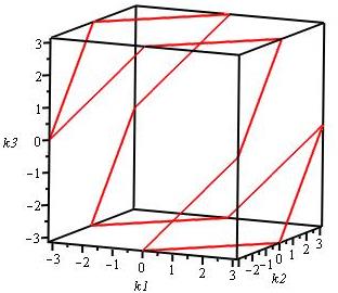
Figure 6. The set $K_{1}^{+}=K_{2}^{-}$ defined by (4.9).

Remark 4.5.

The set $K_{1}^{+}=K_{2}^{-}$ defined by (4.9) is an algebraic curve of co-dimension 2 shown in red line in Fig. 6. The band edges $\lambda_{1}^{+}$ and $\lambda_{2}^{-}$ are degenerate. This example of periodic graphs where the non-degeneracy assumption fails was constructed in [BK20].

Proof. For the diamond lattice ${\mathcal{G}}$, the matrix of the Floquet operator $H(k)$ defined by (1.4) in the standard basis of $\ell^{2}(\{v_{1},v_{2}\})\cong{\mathbb{C}}^{2}$ has the form

$$H(k)=\left(\begin{array}[]{cc}4+q&-1-e^{ik_{1}}-e^{ik_{2}}-e^{ik_{3}}\\ -1-e^{-ik_{1}}-e^{-ik_{2}}-e^{-ik_{3}}&4-q\end{array}\right),$$

$k=(k_{1},k_{2},k_{3})\in{\mathcal{B}}=(-\pi,\pi]^{3}$. The eigenvalues of $H(k)$ are given by

$$\lambda_{j}(k)=4+(-1)^{j}\sqrt{f(k)+q^{2}},\qquad j=1,2,\quad$$

$$\textrm{where}\qquad f(k)=|1+e^{ik_{1}}+e^{ik_{2}}+e^{ik_{3}}|^{2}.$$

We have

$$\textstyle\min\limits_{k\in{\mathcal{B}}}f(k)=f\big{(}K_{1}^{+}\big{)}=0,\qquad\max\limits_{k\in{\mathcal{B}}}f(k)=f(0,0,0)=16,$$

where $K_{1}^{+}$ is defined by (4.9). Then, using the definition of the band edges $\lambda_{j}^{\pm}$ in (1.6), we obtain that the spectrum of $H$ has the form (4.8), (4.9).  $\Box$

Now we prove Example 2.12 describing all subcoverings ${\mathcal{G}}_{\mathfrak{t}}$ of the diamond lattice ${\mathcal{G}}$ isospectral to ${\mathcal{G}}$.

Proof of Example 2.12. Let $\mathfrak{t}=t_{1}\mathfrak{a}_{1}+t_{2}\mathfrak{a}_{2}+t_{3}\mathfrak{a}_{3}$ be a primitive vector of the lattice $\Gamma$. For some $i,j=1,2,3$, $i\neq j$, the numbers $t_{i}$ and $t_{j}$ have the same parity, i.e., $t_{i}+t_{j}$ is even. Let $k_{o}=(k_{o1},k_{o2},k_{o3})$ be defined by

$$k_{oi}=k_{oj}=\pi,\qquad k_{ol}=0,\quad l\in\{1,2,3\}\setminus\{i,j\}.$$

Then $k_{o}\in K_{1}^{+}=K_{2}^{-}$, where $K_{1}^{+}=K_{2}^{-}$ is defined by (4.9) and for $k_{o}$ and ${\mathcal{T}}=(t_{1},t_{2},t_{3})$ the condition (2.5) is fulfilled. For the point $0\in K_{1}^{-}=K_{2}^{+}$ the condition (2.5) is also fulfilled. Thus, due to Corollary 2.5, the diamond lattice ${\mathcal{G}}$ is isospectral to its subcovering ${\mathcal{G}}_{\mathfrak{t}}$, i.e., $\sigma(H)=\sigma(H_{\mathfrak{t}})$.

Now let $\mathfrak{t}=\{\mathfrak{t}_{1},\mathfrak{t}_{2}\}$ be a primitive set of the lattice $\Gamma$, where $\mathfrak{t}_{s}=t_{s1}\mathfrak{a}_{1}+t_{s2}\mathfrak{a}_{2}+t_{s3}\mathfrak{a}_{3}$, $s=1,2$. If for some $i,j=1,2,3$, $i\neq j$, the sum $t_{si}+t_{sj}$ is even for each $s=1,2$, then using the same arguments as above we obtain that ${\mathcal{G}}$ and ${\mathcal{G}}_{\mathfrak{t}}$ are isospectral. Conversely, if ${\mathcal{G}}$ and ${\mathcal{G}}_{\mathfrak{t}}$ are isospectral, then, due to Corollary 2.5,

$$t_{s1}k_{o1}+t_{s2}k_{o2}+t_{s3}k_{o3}\in 2\pi{\mathbb{Z}},\qquad s=1,2,$$ (4.10)

for some $k_{o}=(k_{o1},k_{o2},k_{o3})\in K_{1}^{+}=K_{2}^{-}$. Using the structure of the set $K_{1}^{+}$ (see Fig. 6), we have

$$k_{ol}=\pi,\quad k_{oi}-k_{oj}=\pm\pi,\quad\textrm{for some pairwise distinct}\;i,j,l\in\{1,2,3\}.$$

Substituting this into (4.10) and using that $t_{si}\in{\mathbb{Z}}$, we obtain

$$(t_{si}+t_{sj})k_{oj}+\pi(t_{si}+t_{sl})\in 2\pi{\mathbb{Z}},\qquad s=1,2.$$ (4.11)

We assume that there are no $i,j=1,2,3$, $i\neq j$, such that the sum $t_{si}+t_{sj}$ is even for each $s=1,2$, i.e., for each pair $(i,j)\in\{1,2,3\}^{2}$ with $i\neq j$, at least one of the sums $t_{si}+t_{sj}$, $s=1,2$, is odd. This yields that, up to the permutations of the index $s=1,2$, only the following three cases are possible:

Case	$t_{1i}+t_{1j}$	$t_{2i}+t_{2j}$	$t_{1i}+t_{1l}$	$t_{2i}+t_{2l}$
1	even	odd	odd	even
2	even	odd	odd	odd
3	odd	odd	even	odd

We consider Case 1. Cases 2 and 3 are similar. In Case 1 the conditions (4.11) have the form

$$2n_{1}k_{oj}=(2m_{1}+1)\pi,\qquad(2n_{2}+1)k_{oj}=2m_{2}\pi$$

for some $n_{s},m_{s}\in{\mathbb{Z}}$, $s=1,2$, which yields the contradiction $4n_{1}m_{2}=(2m_{1}+1)(2n_{2}+1)$. Thus, if ${\mathcal{G}}$ and ${\mathcal{G}}_{\mathfrak{t}}$ are isospectral, then for some $i,j=1,2,3$, $i\neq j$, the sum $t_{si}+t_{sj}$ is even for each $s=1,2$.  $\Box$

References

• [A95] Adachi, T. On the spectrum of periodic Schrödinger operators and a tower of coverings. Bull. London Math. Soc. 27 (1995), no. 2, 173–176.
• [AM76] Ashcroft, N.W.; Mermin, N.D. Solid State Physics, Holt, Rinehart and Winston, New York – London, 1976.
• [BCCM22] Berkolaiko, G.; Canzani, Y.; Cox, G.; Marzuola, J.L. A local test for global extrema in the dispersion relation of a periodic graph. Pure Appl. Anal. 4 (2022), no. 2, 257–286.
• [BK13] Berkolaiko, G.; Kuchment, P. Introduction to Quantum Graphs, Mathematical Surveys and Monographs, V. 186 AMS, 2013.
• [BK20] Berkolaiko, G.; Kha, M. Degenerate band edges in periodic quantum graphs. Lett. Math. Phys. 110 (2020), no. 11, 2965–2982.
• [C97] Cassels, J.W.S. An introduction to the geometry of numbers, Springer, Berlin, 1997.
• [D15] Do, N. On the quantum graph spectra of graphyne nanotubes. Anal. Math. Phys. 5 (2015), 39–65.
• [DKS20] Do, N.; Kuchment, P.; Sottile, F. Generic properties of dispersion relations for discrete periodic operators. J. Math. Phys. 61 (2020), no. 10.
• [GKT93] Gieseker, D.; Knörrer, H.; Trubowitz, E. The geometry of algebraic Fermi curves, volume 14 of Perspectives in Mathematics. Academic Press Inc., Boston, MA, 1993.
• [FK18] Filonov, N.; Kachkovskiy, I. On the structure of band edges of 2-dimensional periodic elliptic operators, Acta Math. 221 (2018), no. 1, 59–80.
• [HKSW07] Harrison, J.M.; Kuchment, P.; Sobolev, A.; Winn, B. On occurrence of spectral edges for periodic operators inside the Brillouin zone, J. Phys. A 40 (2007), 7597–7618.
• [HN09] Higuchi, Y.; Nomura, Y. Spectral structure of the Laplacian on a covering graph, Eur. J. Combin. 30 (2009), no. 2, 570–585.
• [HS99] Higuchi, Y.; Shirai, T. A remark on the spectrum of magnetic Laplacian on a graph, the proceedings of TGT10, Yokohama Math. J., 47 (Special issue) (1999), 129–142.
• [HS04] Higuchi, Y.; Shirai, T. Some spectral and geometric properties for infinite graphs, AMS Contemp. Math. 347 (2004), 29–56.
• [HJ85] Horn, R.; Johnson, C. Matrix analysis. Cambridge University Press, 1985.
• [K89] Kappeler, T. Isospectral potentials on a discrete lattice. III, Trans. Amer. Math. Soc. 314 (1989), no. 2, 815–824.
• [KKR17] Kha, M.; Kuchment, P.; Raich, A. Green’s function asymptotics near the internal edges of spectra of periodic elliptic operators. Spectral gap interior. J. Spectr. Theory 7 (2017), no.4, 1171–1233.
• [K18] M. Kha, Greens function asymptotics of periodic elliptic operators on abelian coverings of compact manifolds, J. Funct. Anal. 274 (2018), no. 2, 341–387.
• [KK10] Korotyaev, E.; Kutsenko, A. Zigzag and armchair nanotubes in external fields, Adv. Math. Res. 10 (2010), 273–302.
• [KS19] Korotyaev, E.; Saburova, N. Spectral estimates for Schrödinger operators on periodic discrete graphs, St. Petersburg Math. J. 30 (2019), 667–698.
• [K05] Kuchment, P. Quantum graphs. II. Some spectral properties of quantum and combinatorial graphs. J. Phys. A 38 (2005), no. 22, 4887–4900.
• [KP07] Kuchment, P.; Post., O. On the spectra of carbon nano-structures, Comm. Math. Phys. 275 (2007), no. 3, 805–826.
• [L23] Liu, W. Floquet isospectrality for periodic graph operators, J. Differ. Equ. 374 (2023), 642–653.
• [L24] Liu, W. Fermi isospectrality for discrete periodic Schrödinger operators, Comm. Pure Appl. Math. 77 (2024), 1126–1146.
• [RS78] Reed, M.; Simon, B. Methods of modern mathematical physics, vol.IV. Analysis of operators, Academic Press, New York, 1978.
• [S24] Saburova, N. Asymptotic isospectrality of Schrödinger operators on periodic graphs, Anal. Math. Phys. 14 (2024), no. 74.
• [S13] Sunada, T. Topological crystallography, Surveys Tutorials Appl. Math. Sci., vol. 6, Springer, Tokyo, 2013.
• [SS92] Sy, P.W.; Sunada, T. Discrete Schrödinger operator on a graph, Nagoya Math. J. 125 (1992), 141–150.