GASP: Gaussian Splatting for Physic-Based Simulations

Abstract

Physical simulation is paramount for modeling and utilization of 3D scenes in various real-world applications. However, its integration with state-of-the-art 3D scene rendering techniques such as Gaussian Splatting (GS) remains challenging. Existing models use additional meshing mechanisms, including triangle or tetrahedron meshing, marching cubes, or cage meshes. As an alternative, we can modify the physically grounded Newtonian dynamics to align with 3D Gaussian components. Current models take the first-order approximation of a deformation map, which locally approximates the dynamics by linear transformations. In contrast, our Gaussian Splatting for Physics-Based Simulations (GASP) model uses such a map (without any modifications) and flat Gaussian distributions, which are parameterized by three points (mesh faces). Subsequently, each 3D point (mesh face node) is treated as a discrete entity within a 3D space. Consequently, the problem of modeling Gaussian components is reduced to working with 3D points. Additionally, the information on mesh faces can be used to incorporate further properties into the physical model, facilitating the use of triangles. Resulting solution can be integrated into any physical engine that can be treated as a black box. As demonstrated in our studies, the proposed model exhibits superior performance on a diverse range of benchmark datasets designed for 3D object rendering. Our project page is at: https://waczjoan.github.io/GASP/.

1 Introduction

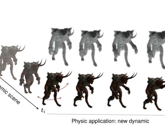
Figure 1: GASP integrates GS with a physical engine to generate realistic simulations. Essentially, GASP utilizes set of triangle meshes to parameterize Gaussian components. This approach reduces modifying Gaussian components to 3D point clouds (consisting of vertices of triangles) processing, enabling efficient and rapid rendering. GASP can model the interaction of objects and work with dynamic scenes.

The recent development of Gaussian Splatting (GS) [13] has greatly influenced the field of computer graphics, enabling the modeling of three-dimensional (3D) scenes from images with annotated camera positions. The GS model represents 3D scenes as a set of 3D Gaussian distributions, which allows for rapid training and rendering. Furthermore, it is relatively straightforward to modify the original GS approach to enable editing [22, 4, 8] and to facilitate the creation of dynamic scenes [21, 11, 14].

Figure 2: GASP produces physical simulations in flat GS. It works with static GS models like GaMeS [22] or dynamic ones like D-MiSo [21]. (In general, GASP can be applied to any GS-based model which uses flat Gaussians.) First, we take the flat Gaussian and convert it to the GaMeS format. Each flat Gaussian component is converted to three points (triangle face). Then, the physical engine is run on a point cloud to obtain trajectories for our 3D model. Finally, we convert points into Gaussian components by reverse GaMeS parametrization.

At the same time, one of the most significant challenges with the GS framework is the incorporation of physics into scenes represented using 3D Gaussian components. It is noteworthy that using a physical engine would pave the way to the implementation of GS in spatial, immersive interfaces such as virtual reality (VR) [12]. Presently, the existing models employ supplementary meshing techniques, including triangle or tetrahedron meshing [2], marching cubes [4], or cage meshes [12]. This approach generates classical mesh-based representations, which are then controlled by a physical engine. Consequently, Gaussian components are adjusted in accordance with mesh-based modifications. While such methods produce satisfactory renderings, they require the implementation of an additional meshing and rendering strategy. Furthermore, modeling tears and cracks represents a challenge, as it is not straightforward to control the behaviors of the mesh when the object is divided. An alternative methodology for addressing the aforementioned issue is to utilize the vanilla GS approach and adapt Newtonian dynamics to accommodate 3D Gaussian components. PhysGaussian [24] employs the first-order approximation of a deformation map. By utilizing such a method, we locally approximate the dynamics through linear transformations. This solution is effective, however, it is contingent upon access to a physical engine in order to apply the modifications and relies on a network approximation.

To address these limitations, we propose the Gaussian Splatting for Physic-Based Simulations (GASP) model (see Fig. 1), which incorporates flat Gaussians [22, 21] with the Material Point Method (MPM) [5] without additional modification (see Fig. 2). Flat Gaussian distributions can be used in GS by applying only minimal changes, such as imposing a zero value on one of the Gaussian components. Such techniques are frequently employed in a multitude of approaches [22, 4, 7], and they facilitate straightforward modifications to the final model. The training and rendering times, as well as the quality of the renderings produced by flat Gaussians, are comparable to those of GS. GASP approach exemplifies the implementation of Newtonian dynamics within the GaMeS framework, thereby illustrating the capacity to integrate these methodologies without the need for external modifications to the physical engine or Gaussian components. More precisely, the model extracts points from GS and applies the Material MPM to control such points. During the simulation process, the Gaussian components associated with each triple of points are recalculated. This process is notably rapid and does not increase rendering costs. At the same time, treating each point as a discrete entity results in the emergence of artifacts. Consequently, we propose a simple modification that utilizes triangles instead of completely disparate points. We use additional rescaling when a triangle undergoes a significant change in size. In practice, GASP can produce high-quality simulations in flat GS, including static and dynamic scenes (see Fig. 3) as well as the interaction of objects (see Fig. 4). This is evidenced by the results of experiments conducted on a range of benchmarks with synthetic (see Fig. 5 ) and real-world data sets (see Fig. 6 ) .

The following constitutes a list of our key contributions:

1. We propose GASP model that incorporates physical properties into a 3D scene representation using GS on both static and dynamic scenes.

2. GASP operates in a direct manner on specific points, thus obviating the necessity for alterations to the physical engine regarded as a black box.

3. GASP does not employ supplementary meshing strategies and instead operates directly with Gaussian distributions.

2 Related Work

The GS representation of 3D scenes is well suited for editing [22, 4, 7] and dynamic scenes modeling [10, 23, 21]. However, the more challenging task is its integration with a physical engine that remains difficult and underexplored.

Figure 3: In this experiment, we added simulated gravity and lowered a rubber teddy bear. As you can see, when the object hits the ground, it changes according to the properties given by the physics engine.

Most of the existing methods use additional strategic tactics to obtain representation well-suited for physical engines. Gaussian Splashing (GSP) [2] is a unified framework that combines 3D Gaussian Splinting (3DGS) and position-based dynamics. During the preprocessing stage, the foreground objects are isolated and reconstructed as a mesh representation. Such a response is then combined with position-based dynamics. Alternatively, we can use cage-based representation [12]. VR-GS [12] combine 3DGS and eXtended Position-based Dynamics (XPBD) [16]. The model starts with scene reconstruction by GS and tetrahedralization. Consequently, we obtain a cage-based representation combined with a physical engine.

All the above models work with an additional meshing strategy. In contrast, PhysGaussian [24] operates directly on Gaussian distributions. The authors of [24] suggest approximating a deformation map using the first-order derivative. This yields a linear transformation capable of modifying Gaussian components. Although this model produces relatively good results, it requires adjustments to the physical engine. In contrast, we propose GASP model which uses a physical engine as a black-box without any modification.

A separate area in the physics modeling involves using diffusion models to generate object dynamics. PhysDreamer [25] introduces a method that provides static 3D objects with interactive dynamics by utilizing object dynamics priors acquired from video generation models. Physics3D [15] learns various physical characteristics of 3D objects using a video diffusion model. DreamPhysics [9] infers physical attributes of 3DGS based on video diffusion priors.

3 GASP Model Overview

Figure 4: GASP reduces the modification of the Gaussian component to 3D point cloud motion. Therefore, we can work with several elements at the same time. In this experiment, we simulate a static mug and a teddy bear made of sand.

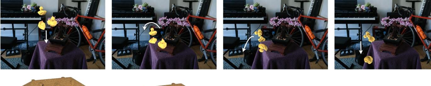
Figure 5: We add small elements to large scenes that interact with them. At the top, we add a rubber duck that falls onto the table. At the bottom, we add the sand-based object. Note that GASP is able to model interaction between 3D objects.

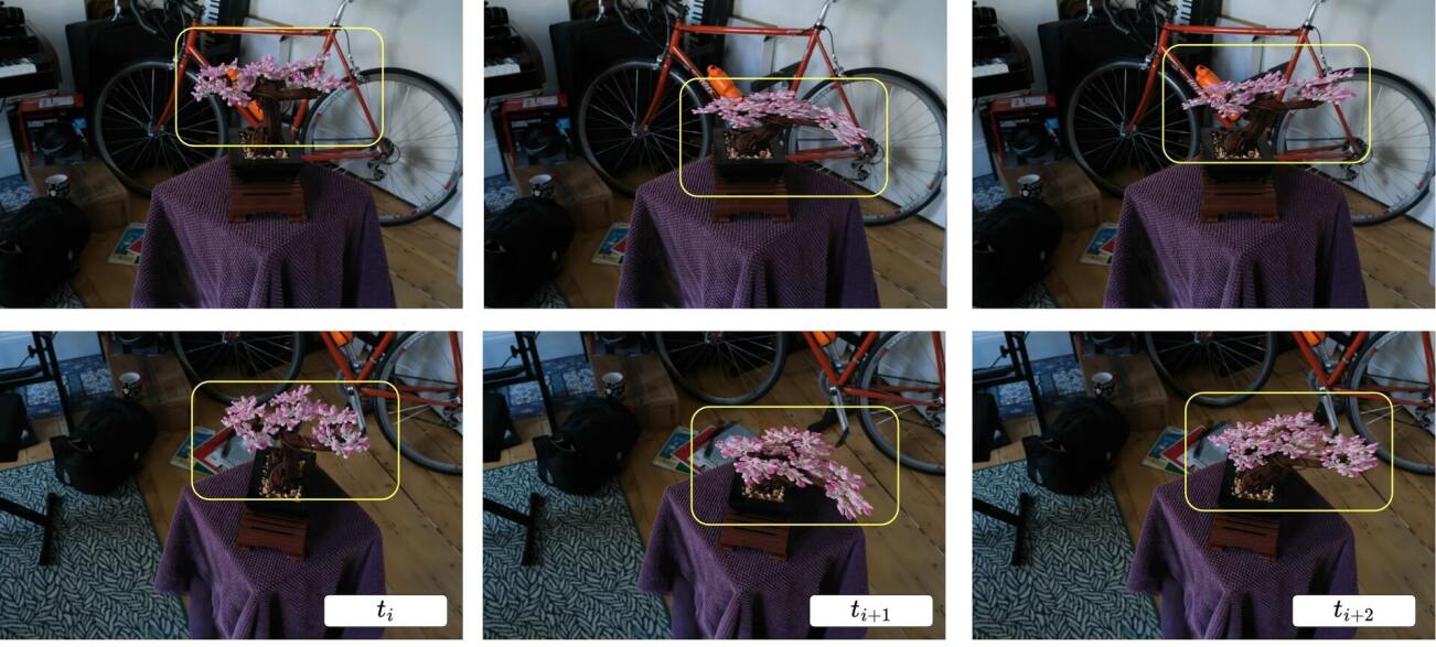
Figure 6: In large scenes, we can select part of the object and add physical properties. In this experiment, we simulate the effect of wind to modify the movement of the bonsai tree.

Figure 7: Blender provides a wide range of physical properties and force sources, including gravity and wind, to create realistic and dynamic animations. In this experiment, we present examples of physical animation in object scenes, showing the versatility of animating both small objects, such as a flower on a table, and large objects, such as a fox’s head dominating the scene.

Here, we present a description of the GASP model. It begins with a general GS model, followed by an examination of the modifications made by GaMeS [22] to the original GS model, which facilitates straightforward adaptations. Subsequently, the classical MPM [5] is outlined, and finally, our own approach combining both GS and MPM is detailed.

Gaussian Splatting

The GS technique [13] generates 3D scenes using a collection of three-dimensional Gaussians:

$$\mathcal{G}=\{(\mathcal{N}({\bf m}_{i},\Sigma_{i}),\sigma_{i},c_{i})\}_{i=1}^{p},$$ (1)

defined by their mean (position) ${\bf m}_{i}$, covariance matrix $\Sigma_{i}$, opacity $\sigma_{i}$, and color $c_{i}$, which is represented using spherical harmonics (SH) [3]. The performance of the GS algorithm is mainly due to its rendering technique, which projects the Gaussian elements into two-dimensional space. Throughout training, all parameters are optimized according to the mean square error (MSE) cost function. Since this training often leads to local minima, GS may utilize additional training methods that include creating, removing, and repositioning components based on the proposed heuristic [13]. This strategy is both fast and efficient.

GaMeS Parametrization of Gaussian Component

In the classical GS model, each element is characterized by a collection of parameters, including a covariance matrix $\Sigma$ which is factored as:

$$\Sigma=RSSR^{T},$$ (2)

where $R$ is the rotation matrix and $S$ is a diagonal matrix containing the scaling parameters. In GaMeS [22], on the other hand, flat Guassians are used:

$$(\mathcal{N}({\bf m},R,S),\sigma,c)$$ (3)

where $S=\mathrm{diag}(s_{1},s_{2},s_{3})$, with $s_{1}=\varepsilon$, and $R$ is the rotation matrix defined as $R=[{\bf r}_{1},{\bf r}_{2},{\bf r}_{3}]$, with ${\bf r}_{i}\in\mathbb{R}^{3}$. Thus, Gaussian components can be visualized through a triangle-face mesh by utilizing the vertices for their parameterization. We refer to this mapping as $\mathcal{T}(\cdot)$. In practice, this parameterization results in a set of triangles, which is referred to as Triangle Soup [18].

To outline the GaMeS parameterization, consider a single Gaussian component $\mathcal{N}({\bf m},R,S)$. Then its face representation $\mathcal{N}(V)$ is based on a triangle:

$$V=[{\bf v}_{1},{\bf v}_{2},{\bf v}_{3}]=\mathcal{T}({\bf m},R,S)$$ (4)

with the vertices defined as:

$${\bf v}_{1}={\bf m},\;\;{\bf v}_{2}={\bf m}+s_{2}{\bf r}_{2},\;\;\textrm{and}\;\;{\bf v}_{3}={\bf m}+s_{3}{\bf r}_{3}.$$ (5)

Conversely, given a face (triangle) representation $V=[{\bf v}_{1},{\bf v}_{2},{\bf v}_{3}]$, we can recover the Gaussian component:

$$\mathcal{N}(\hat{\bf m},\hat{R},\hat{S})=\mathcal{N}(\mathcal{T}^{-1}(V))$$ (6)

through the mean $\hat{\bf m}$, the rotation matrix $\hat{R}=[\hat{\bf r}_{1},\hat{\bf r}_{2},\hat{\bf r}_{3}]$, and the scaling matrix $\hat{S}=\mathrm{diag}(\hat{s}_{1},\hat{s}_{2},\hat{s}_{3})$, where the parameters are defined by the following formulas:

$$\hat{\bf m}={\bf v}_{1},\;\;\hat{\bf r}_{1}=\frac{({\bf v}_{2}-{\bf v}_{1})\times({\bf v}_{3}-{\bf v}_{1})}{\|({\bf v}_{2}-{\bf v}_{1})\times({\bf v}_{3}-{\bf v}_{1})\|},$$ (7)

$$\hat{\bf r}_{2}=\frac{({\bf v}_{2}-{\bf v}_{1})}{\|({\bf v}_{2}-{\bf v}_{1})\|},\;\;\hat{\bf r}_{3}=\mathrm{orth}({\bf v}_{3}-{\bf v}_{1};{\bf r}_{1},{\bf r}_{2}),$$ (8)

$$s_{1}=\varepsilon,\;\;\hat{s}_{2}=\|{\bf v}_{2}-{\bf v}_{1}\|,\;\;\textrm{and}\;\;\hat{s}_{3}=\langle{\bf v}_{3}-{\bf v}_{1},\hat{\bf r}_{3}\rangle.$$ (9)

Here, $\mathrm{orth}(\cdot)$ denotes a single step of the Gram-Schmidt process [1]. Accordingly, the corresponding covariance matrix of a Gaussian distribution is given as:

$$\hat{\Sigma}=\hat{R}\hat{S}\hat{S}\hat{R}^{T}.$$ (10)

Constitutive Model

In alignment with the methodology delineated by [24], the tenets of continuum mechanics form the foundation of the constitutive model. The fundamental principles of continuum mechanics entail the representation of material deformation through the use of a map $\phi$, which transforms points from the initial undeformed material space $X$ to the subsequently deformed world space $x=\phi(X,t)$ at time $t$. This process yields the following deformation gradient:

$$F(X,t)=\nabla_{X}\phi(X,t),$$ (11)

which is used to measure local rotation and strain. The deformation function $\phi$ is subject to changes in accordance with the principles of conservation of mass, conservation of momentum, and the elasto-plastic constitutive relation:

$$\frac{D\rho}{Dt}=0,\;\;\frac{Dv}{Dt}=\frac{1}{\rho}\nabla\cdot\sigma+f,$$ (12)

and

$$\sigma=\frac{1}{\det(F)}\frac{\partial\Psi}{\partial F^{E}}({F^{E}})^{T}.$$ (13)

In this context, $\rho$ and $v$ denote the density and velocity as functions of time $t$ and position $x$, while $\sigma$ is the Cauchy stress tensor, which includes both pressure and shear, and $\nabla\cdot\sigma$ denotes its divergence. Furthermore, $f$ represents a vector that includes all accelerations caused by body forces (e.g. gravitational acceleration). On the other hand, $\Psi$ is the strain energy density function of $F$, which quantifies the amount of non-rigid deformation. Note that in our work, we use a plasticity model in which the deformation gradient is multiplicatively decomposed (following some yield stress condition) into an elastic part $F^{E}$ and a plastic part $F^{P}$, so that $F=F^{E}F^{P}$.

Figure 8: GASP approach operates directly on Gaussian representations without altering the physics-based deformation network. Initially, the 3D objects are depicted as flat Gaussians. GaMeS then converts these Gaussians into triplets (mesh faces). The simulation engine transforms these points following the MPM model. Subsequently, the new points are reassembled into triangles and then into Gaussians. This process is extremely fast, yielding realistic renderings.

Material Point Method

The fundamental premise of the MPM is the utilization of particles, or material points, for the tracking of mass, momentum, and deformation gradient (here, we track rather $F^{E}$ than $F$). From one perspective, the Lagrangian approach enables the monitoring of time-varying characteristics, such as position, velocity, and deformation gradient, in alignment with the mass conservation principle for each particle. This approach ensures the constancy of the overall mass. Conversely, the lack of mesh connectivity between particles represents a substantial challenge in calculating derivatives, which are crucial for stress-based force evaluation (see Equation (13)) and are, in turn, a fundamental component of the momentum conservation principle. This issue can be addressed by employing a regular Eulerian grid as a background and discretizing the Cauchy stress tensor divergence $\nabla\cdot\sigma$ with the use of interpolation functions over the grid in a manner analogous to the standard Finite Element Method (FEM), utilizing the weak form. In this approach, the grid basis functions are dyadic products of one-dimensional cubic B-splines [19].

The MPM algorithm is a three-stage process comprising particle-to-grid transfer, grid update, and grid-to-particle transfer, which are applied in a loop [24]. In the initial stage, mass and momentum are transferred from the particle to the grid. In the subsequent stage, grid velocities are updated based on forces at the next timestep. In the final stage, the updated grid velocities are transferred back to the particles, and then new quantities of the particles are computed.

GASP – Physics in GaMeS

This subsection presents a description of the GASP model. Since the model employs the GaMeS representation of a 3D scene, we postulate that the input comprises a collection of Gaussians:

$$\mathcal{G}=\{(\mathcal{N}({\bf m}_{i},R_{i},S_{i}),\sigma_{i},c_{i})\}_{i=1}^{p},$$ (14)

with means ${\bf m}_{i}$, scaling matrices $S_{i}$, and rotation matrices $R_{i}$. Furthermore, we assume the existence of a deformation map $\phi(X,t)$, which models the behavior of 3D objects. In order to obtain $\phi(X,t)$, it is necessary to have a point cloud that describes 3D objects. As our method employs the GaMeS reparametrization of GS, we are able to transform the mean Gaussian parameters and the covariance matrix into a mesh (triangle soup). In such an instance, we may consider the system $(\mathcal{V},\mathcal{E})$, where:

$$\mathcal{V}=\{V_{i}=\mathcal{T}({\bf m}_{i},R_{i},S_{i})\}_{i=1}^{p}$$ (15)

denotes a collection of vertices, and $\mathcal{E}$ represents the edges obtained via GaMeS. Our physical-based deformation network operates on each point of $V_{i}$ individually. Subsequently, the vertices of the triangle soup can be used as input for the MPM algorithm in conjunction with tools such as the Blender or Taichi libraries (for further details, see the experimental section). It is essential to note that our solution does not entail any modifications to the MPM, in contrast to the Taylor approximation employed in [24]. Consequently, in each time step, the following is obtained:

$$\mathcal{V}_{t}=\{\phi(V_{i},t)\colon V_{i}\in\mathcal{V}\}.$$ (16)

The mesh in time $t$ is then defined by the collection of vertices and edges $(\mathcal{V}_{t},\mathcal{E}_{t})$. In contrast, the reverse parametrization provided by GaMeS can be employed to obtain Gaussian Splatting:

$$\mathcal{G}_{t}=\{(\mathcal{N}(\mathcal{T}^{-1}(\phi(V_{i},t))),\sigma_{i},c_{i})\}_{i=1}^{p}.$$ (17)

It is important to note that processing each vertex of a triangle soup individually is a highly rapid process that treats the physical engine as an opaque black box. The schema of such processes is presented in Fig. 8. Our method is compatible with any physics engine that operates on three-dimensional points. However, the processing of all points separately may yield artifacts. When all points are treated independently during simulation, some elements exhibit considerable fluctuations in velocity. This phenomenon leads to the formation of extensive triangles (mesh faces), which in turn give rise to prominent Gaussian components, as illustrated in Fig. 9. To mitigate this effect, our approach employs a straightforward yet highly effective technique (correction algorithm). Specifically, we monitor the distance between vertices of the face representation $V=[{\bf v}_{1},{\bf v}_{2},{\bf v}_{3}]$ of a Gaussian component $\mathcal{N}({\bf m},R,S)$. It should be noticed that in the case of GaMeS transformation, the first vertex is equal to the center of the distribution (${\bf v}_{1}={\bf m}$), while the two subsequent vertices are located on the main components of the ellipses that describe the distribution (${\bf v}_{2}={\bf m}+s_{2}{\bf r}_{2}$, ${\bf v}_{3}={\bf m}+s_{3}{\bf r}_{3}$). Consequently, if the distance between the transformed mesh nodes is considerably greater than that of the original nodes, i.e.:

$$\|\phi({\bf v}_{1},t)-\phi({\bf v}_{i},t)\|>\alpha\|{\bf v}_{1}-{\bf v}_{i}\|\;\;\mbox{for}\;\;i=2,3,$$ (18)

where $\alpha$ is a hyperparameter, we automatically assert that the value of $s_{i}$ should be identical to that of the original value times $\alpha$. This is illustrated in Fig. 10. It should be noted that throughout the full simulation, both the mesh and GS are accessible, enabling real-time rendering.

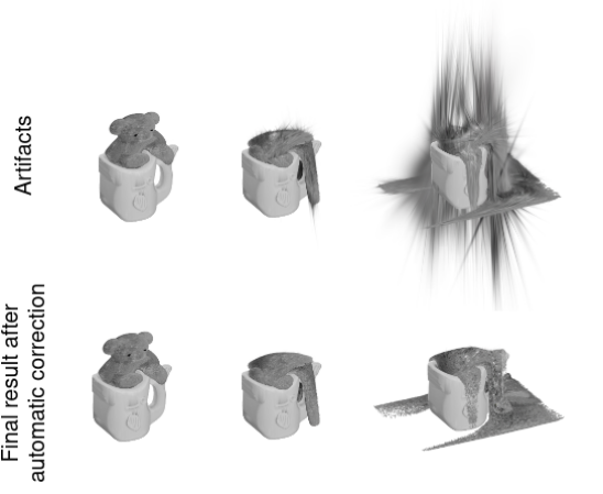
Figure 9: Comparison of physical animation models, illustrating the effects of applying an algorithm for correcting points used in simulation. The left side demonstrates a simulation without the correction algorithm, while the right side shows the enhanced accuracy and stability achieved using Taichi elements with the correction algorithm applied.

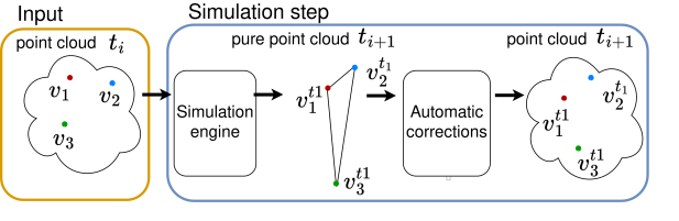
Figure 10: GASP works directly on points cloud extracted from flat Gaussians. In practice, physical engine moves all particles independently, which can produce artifacts. Therefore, we use a correction algorithm to control the distance of points from each other. If some points are moved extremely far, we automatically correct such behaviors by clipping parameters $S$ in GS.

GASP for Dynamic Scene

GASP is a natural combination of a physical engine dedicated to points and Gaussian Splatting with flat Gaussians. The reparametrization in GaMeS can be applied to a multitude of disparate methodologies, with a particular focus on flat Gaussian methods [4, 7]. Moreover, it can be employed for dynamic Gaussian Splatting. In [21], D-MiSo model is introduced, which uses flat Gaussians for the modeling of dynamic scenes. Such representations can be utilized in conjunction with the aforementioned approach. In the D-MiSo framework, two distinct types of Gaussians and two deformable networks are employed. In the process of inference, only sub-Gaussians are employed, which are modified by deformable function composition $\psi(v,s)$, i.e.,

$$\mathcal{G}_{\text{D-MiSo}}=\left\{\left(\mathcal{N}_{sub}\left(\psi(V_{j}^{i},s)\right),\sigma_{i},c_{i}\right)\right\}_{i=1}^{p},$$ (19)

where $s$ represents a time value derived from the dynamics observed in the scenes. In our solution, we can incorporate a deformation map $\phi(X,t)$, which originates from the physics simulator. Consequently, GASP for the dynamic scene is given as follows:

$$\mathcal{G}_{t}=\left\{\left(\mathcal{N}_{sub}\left(\phi(\psi(V_{j}^{i},s),t)\right),\sigma_{i},c_{i}\right)\right\}_{i=1}^{p},$$ (20)

where $s$ represents time in the dynamic scene and $t$ denotes time in the simulation.

4 Experiments

This experimental section demonstrates that GASP is a universal method that can be applied to both small objects and large scenes. Furthermore, it allows for the modeling of interactions between objects and breaking them into pieces. GASP is also capable of working with dynamic scenes.

Static Objects

The Shiny Dataset [20] contains examples of static objects with varying textures. In such a case, all Gaussian components are converted to GaMeS-based representations, after which training of the physical engine is conducted. Specifically, GASP is employed to move the these representations in accordance with a dynamic function. As can be observed in Fig. 1 and Fig. 3, the model is capable of producing high-quality animation renders. In Tab. 1(a), we compare the FID score obtained by GS and GaMeS on static scenes to GASP during simulations. As we can see, our simulation obtained a slightly worse score but still with high-quality renders.

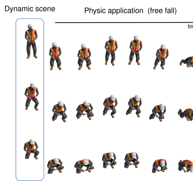
Figure 11: Controlling animations using physics engines allows for application to dynamic objects. This figure compares animations of a dynamic object at three different times under the same physical parameters. This experiment uses GASP integrated with the D-MiSo model [21].

Dynamic Objects

We show that our pipeline also works on dynamic scenes using sample objects from the D-NeRF dataset [17]. We use D-MiSo [21] to model dynamic scenes by flat Gaussians. Then we select random frame and use physical engine. Fig. 1 and Fig. 11 present how the objects change according to physical engine and timeline. In Tab. 1(b), we present the FID score in three different time-steps of dynamic scenes. As we can see, our renders obtain similar scores, which means that our model produces consistent simulations.s.

Multiple Objects

Our model can model the interaction of static objects. In this case, each element of the scene is trained separately. Also, the properties of each component are specified by different parameters. In Fig. 4 we show a sand-based teddy bear and a glass cup. As we can see, the sand falls smoothly into the cup. Let us take the example of interaction between two objects. In Fig. 9 we show how our model handles the formation of artifacts. In Fig. 5 we integrate small duck objects into a full scene. As we can see, the ducks bounce off the table and fall to the ground. Fig. 1 demonstrates the application of physics to two interacting objects: a falling ball and a car reacting to its impact.

Breaking Objects

GASP uses triangle soup to represent flat Gaussians, so we can easily break objects into pieces. In Fig. 12 we show how a cup can be broken. It is important to note that we need a special physics engine to model such a situation. In this example we use additional information about the mesh to train GaMeS on mesh faces (for details see [22]). In this case, Gaussians lie perfectly on the mesh. The initial Gaussian splatting must be trained with additional conditions, but the final GASP modifications are applied analogously to the previous examples (except that here the model is parameterized by mesh).

Figure 12: In this experiment, we create a simulation of a shattering cup using physics simulations. The GaMeS model is used to create a scenario where Gaussians parameters can be adjusted using the mesh.

Model of Physics

We demonstrate that physics modeling can function as a black box by using two different simulation approaches.

Taichi$\_$elements is a highly efficient physics engine for the simulation of multi-material continuum mechanics, originally developed in Python using taichi[6], which is designed for high-performance parallel numerical computation. It supports multiple materials, including water, elastic objects, snow, and sand.

Blender is the most popular open source application for a variety of 3D computer graphics tasks. Our GaMeS-based representation can be imported into Blender, where it can be seen as a triangle soup. Using tools such as mesh deformation, we were able to smoothly simulate soft body physics. The simulation objects were then exported and rendered using the GS renderer. Due to the high speed of the latter process, this method allows us to render our simulation faster for realistic scenes than in the case of using traditional 3D methods in Blender. The animations created in Blender utilized the ”Lattice” and ”Mesh Deform” modifiers, with the mesh being defined by the user, such as a sphere or a cube.

Table 1: Frechet Inception Distance (FID) is calculated in two settings: static scenes (Bonsai, Fox) and dynamic scene standup. GASP obtains slightly worse FID concerning static model GS and GaMeS; see Tab. 1(a). GASP gives similar FID across dynamic scenes; see Tab. 1(b).

	FID ($\downarrow$)
Method	Bonsai	Fox
3DGS	19.71	51.04
GaMeS	19.64	47.62
Ours	38.33	88.59

(a) Comparison of FID score obtained by classical GS and GaMeS for static scenes and renders on images taken across GASP simulation.

Frame	FID ($\downarrow$)
Standup
Start	133.55
Mid	112.79
End	142.90

(b) FID score for three different times obtained by GASP. As we can see, the simulation is consistent across dynamic scenes.

5 Conclusion

In this paper, we introduce GASP, a model that integrates high-quality rendering with accurate physical simulation. By leveraging a GaMeS-based representation of objects, our approach enables the simulation of basic phenomena, such as crushing, and more complex scenarios, including cracking and rainfall. This demonstrates the model’s versatility and effectiveness in handling a wide range of physical interactions within simulated environments. Experimental section, shows that GASP work in many difference scenario and produce high quality simulations.

Limitations

Our model produces artifacts when the simulation changes shapes essentially.

References

- [1] Ake Björck. Numerics of Gram-Schmidt orthogonalization. Linear Algebra and Its Applications, 197:297–316, 1994.
- [2] Yutao Feng, Xiang Feng, Yintong Shang, Ying Jiang, Chang Yu, Zeshun Zong, Tianjia Shao, Hongzhi Wu, Kun Zhou, Chenfanfu Jiang, et al. Gaussian splashing: Dynamic fluid synthesis with gaussian splatting. arXiv preprint arXiv:2401.15318, 2024.
- [3] Sara Fridovich-Keil, Alex Yu, Matthew Tancik, Qinhong Chen, Benjamin Recht, and Angjoo Kanazawa. Plenoxels: Radiance fields without neural networks. In CVPR, pages 5501–5510, 2022.
- [4] Antoine Guédon and Vincent Lepetit. Sugar: Surface-aligned gaussian splatting for efficient 3d mesh reconstruction and high-quality mesh rendering. In Proceedings of the IEEE/CVF Conference on Computer Vision and Pattern Recognition, pages 5354–5363, 2024.
- [5] Yuanming Hu, Yu Fang, Ziheng Ge, Ziyin Qu, Yixin Zhu, Andre Pradhana, and Chenfanfu Jiang. A moving least squares material point method with displacement discontinuity and two-way rigid body coupling. ACM Transactions on Graphics (TOG), 37(4):1–14, 2018.
- [6] Yuanming Hu, Tzu-Mao Li, Luke Anderson, Jonathan Ragan-Kelley, and Frédo Durand. Taichi: a language for high-performance computation on spatially sparse data structures. ACM Transactions on Graphics (TOG), 38(6):201, 2019.
- [7] Binbin Huang, Zehao Yu, Anpei Chen, Andreas Geiger, and Shenghua Gao. 2d gaussian splatting for geometrically accurate radiance fields. In ACM SIGGRAPH 2024 Conference Papers, pages 1–11, 2024.
- [8] Jiajun Huang and Hongchuan Yu. Gsdeformer: Direct cage-based deformation for 3d gaussian splatting. arXiv preprint arXiv:2405.15491, 2024.
- [9] Tianyu Huang, Yihan Zeng, Hui Li, Wangmeng Zuo, and Rynson WH Lau. Dreamphysics: Learning physical properties of dynamic 3d gaussians with video diffusion priors. arXiv preprint arXiv:2406.01476, 2024.
- [10] Yi-Hua Huang, Yang-Tian Sun, Ziyi Yang, Xiaoyang Lyu, Yan-Pei Cao, and Xiaojuan Qi. Sc-gs: Sparse-controlled gaussian splatting for editable dynamic scenes. arXiv preprint arXiv:2312.14937, 2023.
- [11] Yi-Hua Huang, Yang-Tian Sun, Ziyi Yang, Xiaoyang Lyu, Yan-Pei Cao, and Xiaojuan Qi. Sc-gs: Sparse-controlled gaussian splatting for editable dynamic scenes. In Proceedings of the IEEE/CVF Conference on Computer Vision and Pattern Recognition, pages 4220–4230, 2024.
- [12] Ying Jiang, Chang Yu, Tianyi Xie, Xuan Li, Yutao Feng, Huamin Wang, Minchen Li, Henry Lau, Feng Gao, Yin Yang, et al. Vr-gs: a physical dynamics-aware interactive gaussian splatting system in virtual reality. In ACM SIGGRAPH 2024 Conference Papers, pages 1–1, 2024.
- [13] Bernhard Kerbl, Georgios Kopanas, Thomas Leimkühler, and George Drettakis. 3d gaussian splatting for real-time radiance field rendering. ACM Trans. Graph., 42(4):139–1, 2023.
- [14] Agelos Kratimenos, Jiahui Lei, and Kostas Daniilidis. Dynmf: Neural motion factorization for real-time dynamic view synthesis with 3d gaussian splatting. arXiv preprint arXiv:2312.00112, 2023.
- [15] Fangfu Liu, Hanyang Wang, Shunyu Yao, Shengjun Zhang, Jie Zhou, and Yueqi Duan. Physics3d: Learning physical properties of 3d gaussians via video diffusion. arXiv preprint arXiv:2406.04338, 2024.
- [16] Miles Macklin, Matthias Müller, and Nuttapong Chentanez. Xpbd: position-based simulation of compliant constrained dynamics. In Proceedings of the 9th International Conference on Motion in Games, pages 49–54, 2016.
- [17] Albert Pumarola, Enric Corona, Gerard Pons-Moll, and Francesc Moreno-Noguer. D-NeRF: Neural Radiance Fields for Dynamic Scenes. In Proceedings of the IEEE/CVF Conference on Computer Vision and Pattern Recognition, 2020.
- [18] Hayong Shin, J.C. Park, B.K. Choi, Y.C. Chung, and S. Rhee. Efficient topology construction from triangle soup. In Geometric Modeling and Processing, 2004. Proceedings, pages 359–364, 2004.
- [19] Michael Steffen, Robert M Kirby, and Martin Berzins. Analysis and reduction of quadrature errors in the material point method (mpm). International journal for numerical methods in engineering, 76(6):922–948, 2008.
- [20] Dor Verbin, Peter Hedman, Ben Mildenhall, Todd Zickler, Jonathan T. Barron, and Pratul P. Srinivasan. Ref-NeRF: Structured view-dependent appearance for neural radiance fields. CVPR, 2022.
- [21] Joanna Waczyńska, Piotr Borycki, Joanna Kaleta, Sławomir Tadeja, and Przemysław Spurek. D-miso: Editing dynamic 3d scenes using multi-gaussians soup. arXiv preprint arXiv:2405.14276, 2024.
- [22] Joanna Waczyńska, Piotr Borycki, Sławomir Tadeja, Jacek Tabor, and Przemysław Spurek. Games: Mesh-based adapting and modification of gaussian splatting. arXiv preprint arXiv:2402.01459, 2024.
- [23] Guanjun Wu, Taoran Yi, Jiemin Fang, Lingxi Xie, Xiaopeng Zhang, Wei Wei, Wenyu Liu, Qi Tian, and Wang Xinggang. 4d gaussian splatting for real-time dynamic scene rendering. arXiv preprint arXiv:2310.08528, 2023.
- [24] Tianyi Xie, Zeshun Zong, Yuxing Qiu, Xuan Li, Yutao Feng, Yin Yang, and Chenfanfu Jiang. PhysGaussian: Physics-integrated 3D gaussians for generative dynamics. In Proceedings of the IEEE/CVF Conference on Computer Vision and Pattern Recognition, pages 4389–4398, 2024.
- [25] Tianyuan Zhang, Hong-Xing Yu, Rundi Wu, Brandon Y Feng, Changxi Zheng, Noah Snavely, Jiajun Wu, and William T Freeman. Physdreamer: Physics-based interaction with 3d objects via video generation. arXiv preprint arXiv:2404.13026, 2024.