High-fidelity heralded quantum state preparation and measurement
Abstract
We present a novel protocol for high-fidelity qubit state preparation and measurement (SPAM) that combines standard SPAM methods with a series of in-sequence measurements to detect and remove errors. The protocol can be applied in any quantum system with a long-lived (metastable) level and a means to detect population outside of this level without coupling to it. We demonstrate the use of the protocol for three different qubit encodings in a single trapped ion. For all three, we achieve the lowest reported SPAM infidelities of (optical qubit), (metastable-level qubit), and (ground-level qubit).
I Introduction
One of the requirements for building a quantum computer (QC) is the ability to perform qubit state preparation and measurement (SPAM) with low error [1]. QC platforms based on atomic qubits allow for high-fidelity SPAM using optical pumping [2, 3, 4] and state-selective fluorescence [5, 6, 7, 8], avoiding the tradeoffs between SPAM fidelity and gate fidelity common for solid-state platforms [9, 10, 11]. Following early work on high-fidelity SPAM in [12], multiple techniques have been developed to extend these methods onto atomic qubits with more complex internal structure, such as ions with nuclear spin [13, 14, 15], which can be advantageous for quantum computing, sensing, and timekeeping [16, 14]. While previous experiments reported SPAM errors as low as [13], high-fidelity qubit SPAM remains in general challenging and resource-intensive, with error sources including impure laser polarization, imperfect transfer pulses, and finite atomic lifetime.
In this work, we propose a novel protocol that alleviates many of these challenges, allowing for high-fidelity SPAM of a broad class of qubits in atomic and atom-like systems. We combine the standard SPAM methods with a number of mid-circuit non-demolition (QND) measurements [17, 18] that allow us to detect and correct a broad range of errors. Specifically, these measurements are designed to raise a flag when a SPAM error occurs. We can use these flags to reject the corresponding experiment shot through post-selection [19], repeat the cycle until no flag is raised (repeat-until-success) [20] or incorporate them into the analysis of the algorithm’s output [21]. The protocol can be applied to different qubit encodings, such as optical (O), metastable (M), and ground (G) qubits in atomic systems [22] and in any platform with a metastable manifold and a measurement that can detect population outside this manifold. Our protocol is closely connected to the idea of erasure conversion of leakage errors in quantum operations [23, 24, 25, 26, 27].
We implement the protocol on three types of qubits in a single trapped ion, achieving the lowest SPAM error reported to date, for any qubit, on all of them – O: , M: , and G: . We find that the in-sequence QND measurements reduce the SPAM error by over four orders of magnitude while only rejecting of the shots. These results demonstrate the versatility and error resilience of our SPAM protocol.
II SPAM Protocol
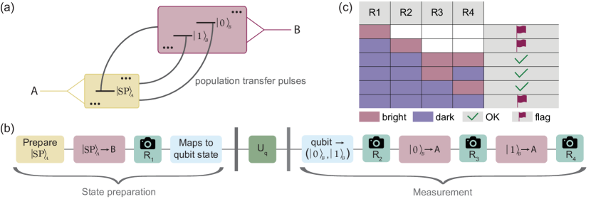
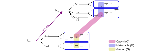
Consider a multi-level quantum system with two long-lived manifolds, A and B, connected by population transfer channels, schematically represented in Fig. 1(a). The aim of our protocol is to prepare and measure a qubit encoded in states somewhere within and . This problem setting is motivated by the structure of many atomic qubits, where laser pulses can be used to transfer population between ground states (in ) and metastable states (in ) [28, 29]. Depending on the application, it may be desirable to encode both qubit states in the ground level (qubit type ), or in the metastable level (qubit type ), or to place one qubit state in and one in (qubit type ) [22]. In this section, we describe the SPAM protocol in a general manner, independent of the quantum system or qubit encoding. In the subsequent section, we demonstrate its performance with all three qubit encodings in a single trapped ion.
Our protocol relies on three capabilities. First, we must be able to detect the population within using some physical process that does not couple to states within . Henceforth, we will call this process population detection to distinguish it from quantum measurement. We label the outcome of population detection as bright if we detect population within and as dark otherwise. Second, we must be able to transfer the population between individual states in and (see below). Third, we are ideally able to initialize the majority of the population in some state in . In our protocol, population detection is used to flag errors during population initialization and population transfer, as well as leakage errors that leave population outside of the qubit manifold. As a result, the SPAM fidelity depends predominantly on the population detection fidelity, while errors during other steps mainly lead to an effective slowdown of computation.
The full SPAM sequence, implemented in a quantum system with the above properties, is shown in Fig. 1(b). We split the protocol into a state preparation part and a measurement part, in between which a desired quantum computation would be implemented. The state preparation part of the protocol starts with initializing the system in a well-defined state using standard methods — for example, optical pumping in the case of an atomic system. This is followed by transferring the population from to any state in . We then perform a population detection step () and raise an error flag in the case of a bright outcome, signifying population left within . This step thus eliminates errors stemming from both imperfect initialization of the system into and imperfect population transfer from into . Finally, if the state we transferred to in is not part of the qubit manifold, we apply additional transfer pulses to move the population to either or , completing the state preparation sequence.
We now describe the measurement part of the protocol. If the qubit is not fully encoded within , we apply transfer pulses to move the population from into and from into , where and are both in as in Fig. 1(a). We then perform a population detection step, in Fig. 1(b). At this stage, we expect all population to be in , so detecting population in (bright outcome) indicates an error. This step flags errors due to leakage from the qubit manifold into – for example, the spontaneous decay of into [28], as well as errors due to imperfect population transfer in the previous steps. After this step, the population in is transferred to a state in and a population detection step, in Fig. 1(b), is carried out again. The outcome is used to infer the quantum measurement result, where a bright outcome corresponds to the measurement result and a dark outcome corresponds to the measurement result . Finally, the state is transferred to a state in and a final population detection step, in Fig. 1(b), is carried out. As the qubit has to be either in the state or the state , either or has to result in a bright measurement outcome. Measuring dark both times suggests that the population is left in due to imperfect population transfer to , leakage out of the qubit manifold but still within , or a total qubit loss. In any case, the error flag is raised.
The complete truth table for deciding whether to raise a flag based on the outcomes of the four population detection steps is shown in Fig. 1(c). This protocol allows us to detect the most common sources of error in qubit SPAM. It thus eliminates the dependence of the SPAM fidelity on the population transfer and population initialization quality and makes it dependent only on the population detection quality, which can be made very high and very robust to drifts [30].
Assuming perfect population detection, there are only two types of physical errors that the protocol cannot detect. The first is population transfer in or out of the wrong qubit state, e.g. mapping onto instead of . The second is the leakage of population from to between and or during . This would result in a bright outcome of , leading us to wrongly conclude a measurement result .
There are two possible ways of dealing with shots where the error flag was raised. First, it is possible to let the computation continue deterministically and discard the results of flagged shots in the data analysis stage, a technique known as post-selection [19]. Alternatively, the computation flow can be adapted in real-time, for example, by repeating state preparation until success, or up to a fixed maximum number of attempts [20]. While the measurement sequence cannot be repeated until success, it can be used to detect errors and convert them into erasures, which are some of the most straightforward errors to correct using QEC [31, 32, 33, 23]. The real-time adaptive control minimizes the computational slowdown caused by data rejection, which makes it particularly useful for deep circuits and large registers. On the other hand, deterministic operation with post-selection poses minimal requirements on the experimental control system and allows for the lowest error rates, making it useful for near-term algorithms with small-scale QCs.
III Protocol implementation
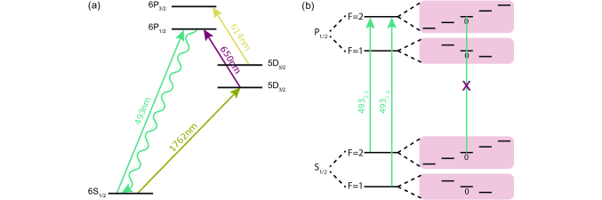
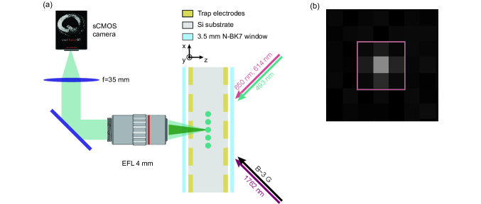
We implement the SPAM protocol in a single ion in a Paul trap, using an experimental setup similar to the one previously described in [34, 35, 36] (see also Sec. S2). We identify the manifolds and with the levels and in , respectively (see Sec. S1 for a complete level diagram). We benchmark the protocol on the three aforementioned qubit types, using encodings O: , M: , and G: .
Population initialization is performed by turning on -polarized light resonant with the and transitions for (see Sec. S1) [13]. We measure a state initialization error of (see Sec. S5), which we attribute to polarization impurity of the beam and off-resonant excitation of the transition.
Population transfer is performed using coherent laser pulses at resonant with individual transitions. The specific transitions addressed differ depending on the qubit encoding and are listed in detail in Sec. S3. The average duration of the pulses is . Individual transfer pulses were measured to have an error rate in the range of (see Sec. S5), largely limited by magnetic field noise and laser phase noise. Further details on the experimental setup can be found in Sec. S2 and Ref. [37].
Population detection is performed using a laser to continuously drive the cycling transition and imaging the scattered photons on a scientific CMOS (sCMOS) camera (see Sec. S2). We use a laser detuning of relative to the measured line centre [38] and a power of , where the saturation intensity is as defined in Ref. [39] (see Sec. S4.1 and Ref. [37]). We collect the photons emitted by the ion on a camera. The camera exposure time is . We categorize the outcome of a population detection as bright or dark by comparing the number of camera counts to a pre-calibrated threshold (see Sec. S4.1 and Ref. [37]). There are two contributions to the population detection error. The first is the optical detection fidelity – the probability that the detection of an ion in the level results in a bright outcome, and the probability that the detection of an ion in the level, which remained in the level during the detection pulse (or equivalently the lack of an ion), results in a dark outcome. We measure this as described in Sec. S4, finding an optical detection error of on the bright state and on the dark state. The second contribution is the probability of decay of the metastable level during the population detection pulse, which we measure as . This agrees with the measured lifetime of the metastable level of (see Sec. S4.2). The above measurements lead to an expected average population detection error of (see Sec. S4 for details).
We benchmark the SPAM protocol using a sequence similar to Fig. 1, with a few modifications. At the start of each shot, the ion is Doppler-cooled [40, 41, 42], and a population detection step is executed to verify the presence of an ion. We then Doppler-cool the ion again and perform the state preparation sequence, followed by the measurement sequence. At the end of the protocol, we deshelve the population out of (see Sec. S1) and perform a final population detection step to confirm the ion remained in the trap during the experiment. Hence, in addition to the rules in the table in Fig. 1(c), we also flag any shots where the result of either or is dark. Afterwards, we discard the shots where a flag was raised using post-selection. We interleave the attempts to prepare with attempts to prepare and record the SPAM fidelity, which is the probability that the measurement outcome matches the intended value [43]. Despite performing a total of six population detection steps per shot, we expect the average SPAM error to be equal to that of one population detection, i.e. . The detailed error budget for the protocol is presented in Sec. S4.
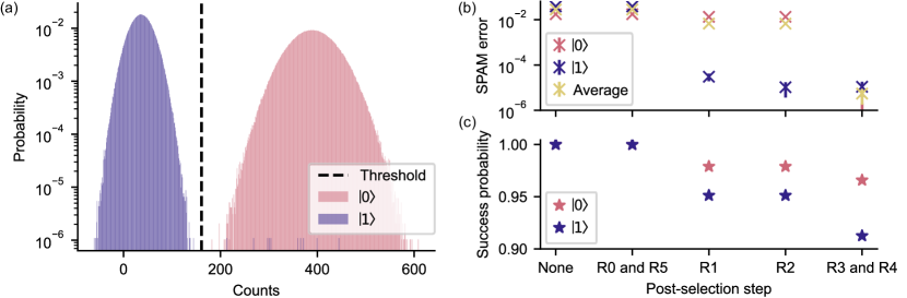
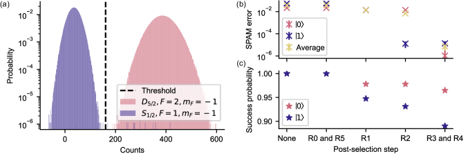
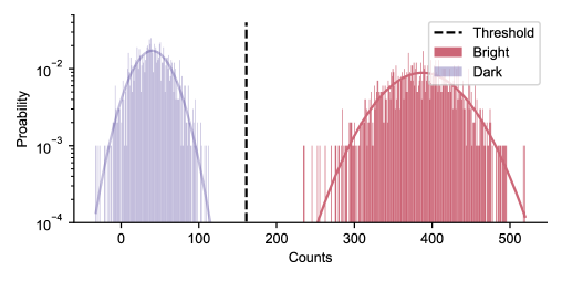
The experimental results for the metastable qubit in are summarised in Fig. 2. We repeat the protocol times for each of the two qubit states. In Fig. 2(a), we show the observed counts during population detection when preparing and after post-selection according to the truth table in Fig. 1(c). The histograms demonstrate that we can achieve excellent population detection in our experiment, which is the core requirement for the high-fidelity implementation of our protocol. In Fig. 2(b) we show the reduction of the average SPAM error after each post-selection step. We find that, without any post-selection, this data exhibits a SPAM error of for and for , giving an average error of . After all post-selection steps, the SPAM error is reduced down to the final value of for and for , giving an average SPAM error of . This agrees with the expected error of . The measured error asymmetry for and is caused by the fact that can decay to but not the other way around. This asymmetry can be exploited to reduce average SPAM errors in QC applications where different measurement outcomes are not equally likely, such as in QEC [44, 24].
In Fig. 2(c), we plot the SPAM success probability (or equivalently the effective computation slowdown rate) after each post-selection step. We find that, while post-section reduces the SPAM error by over four orders of magnitude, it does so while discarding of experimental shots. We note that, due to the different population transfer pulses experiencing different errors (see Sec. S5), qubit states are discarded with unequal probabilities. This does not affect the SPAM fidelity but can bias the results of quantum computing applications that require estimating observable averages [45, 46, 47, 48]. This issue can be corrected by alternating the definition of and for each shot or by carefully measuring the data rejection rate for each qubit state and inverting it in post-processing, see Sec. S6 for details.
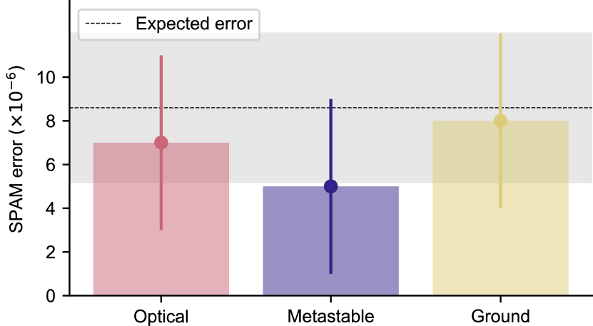
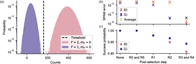
Finally, we repeat the SPAM error measurement for the ground and optical qubit encodings. The results are shown in Fig. 3. As expected from the model, we find that the SPAM fidelities on all three qubit types are the same within experimental uncertainty. Averaged over all three encodings, we record a mean SPAM error of , a record for any qubit in any platform. This demonstrates the encoding flexibility offered by our protocol – as long as a metastable manifold is available, it can be exploited for high-fidelity SPAM, regardless of whether it is part of the qubit encoding.
IV Conclusion
We have developed a new protocol for qubit SPAM that uses a series of mid-circuit QND measurements to effectively detect and flag errors. As a result, the SPAM fidelity depends predominantly on the QND measurement fidelity, which can typically be made very high and robust. Our experimental results with a single trapped ion show that this protocol achieves state-of-the-art performance across three different qubit encodings, demonstrating its versatility.
The only requirement for applying this protocol is a quantum system with a metastable structure as shown Fig. 1(a), which is common to many quantum computing platforms. This makes the protocol highly general, and applicable to a wide range of systems – including both natural and artificial atoms [49, 50] – and encodings, whether based on qubits or qudits [51, 52, 53, 54, 55]. Our protocol can also be applied to atomic and molecular experiments beyond QC, e.g. in precision measurements [56, 57]. Finally, as the capabilities needed to implement the individual steps of our protocol are typically already available in QC setups, we anticipate that our method can be straightforwardly deployed to improve the performance of many existing systems.
Acknowledgments
The authors thank Peter Drmota, David Nadlinger, David Allcock, and David Lucas for helpful discussions. This work was supported by a UKRI FL Fellowship (MR/S03238X/1). ASS acknowledges funding from the JT Hamilton scholarship from Balliol College, Oxford. SMD acknowledges funding from the Jowett scholarship from Balliol College, Oxford.
Competing interests
ASS, FP, and MM are employees of Oxford Ionics Ltd. CJB is a director of Oxford Ionics Ltd. The remaining authors declare no competing interests.
References
- DiVincenzo [2000] D. P. DiVincenzo, Fortschritte der Physik 48, 771 (2000).
- Kastler [1950] A. Kastler, Journal de Physique et le Radium 11, 255 (1950).
- Brossel et al. [1952] J. Brossel, A. Kastler, and J. Winter, Journal de Physique et le Radium 13, 668 (1952).
- Hawkins and Dicke [1953] W. B. Hawkins and R. H. Dicke, Physical Review 91, 1008 (1953).
- Acton et al. [2006] M. Acton, K.-A. Brickman, P. C. Haljan, P. J. Lee, L. Deslauriers, and C. Monroe, “Near-Perfect Simultaneous Measurement of a Qubit Register,” (2006), arXiv:quant-ph/0511257.
- Nagourney et al. [1986] W. Nagourney, J. Sandberg, and H. Dehmelt, Physical Review Letters 56, 2797 (1986).
- Sauter et al. [1986] T. Sauter, W. Neuhauser, R. Blatt, and P. E. Toschek, Physical Review Letters 57, 1696 (1986).
- Bergquist et al. [1986] J. C. Bergquist, R. G. Hulet, W. M. Itano, and D. J. Wineland, Physical Review Letters 57, 1699 (1986).
- Purcell et al. [1946] E. M. Purcell, H. C. Torrey, and R. V. Pound, Physical Review 69, 37 (1946).
- Reed et al. [2010] M. D. Reed, B. R. Johnson, A. A. Houck, L. DiCarlo, J. M. Chow, D. I. Schuster, L. Frunzio, and R. J. Schoelkopf, Applied Physics Letters 96, 203110 (2010).
- Walter et al. [2017] T. Walter, P. Kurpiers, S. Gasparinetti, P. Magnard, A. Potočnik, Y. Salathé, M. Pechal, M. Mondal, M. Oppliger, C. Eichler, and A. Wallraff, Physical Review Applied 7, 054020 (2017).
- Myerson et al. [2008] A. H. Myerson, D. J. Szwer, S. C. Webster, D. T. C. Allcock, M. J. Curtis, G. Imreh, J. A. Sherman, D. N. Stacey, A. M. Steane, and D. M. Lucas, Physical Review Letters 100, 200502 (2008).
- An et al. [2022] F. A. An, A. Ransford, A. Schaffer, L. R. Sletten, J. Gaebler, J. Hostetter, and G. Vittorini, Physical Review Letters 129, 130501 (2022).
- Harty et al. [2014] T. Harty, D. Allcock, C. Ballance, L. Guidoni, H. Janacek, N. Linke, D. Stacey, and D. Lucas, Physical Review Letters 113, 220501 (2014).
- Leu et al. [2024] A. D. Leu, M. C. Smith, M. F. Gely, and D. M. Lucas, “Polarisation-insensitive state preparation for trapped-ion hyperfine qubits,” (2024), arXiv:2406.14448.
- Guggemos et al. [2019] M. Guggemos, M. Guevara-Bertsch, D. Heinrich, O. A. Herrera-Sancho, Y. Colombe, R. Blatt, and C. F. Roos, New Journal of Physics 21, 103003 (2019).
- Grangier et al. [1998] P. Grangier, J. A. Levenson, and J.-P. Poizat, Nature 396, 537 (1998).
- Negnevitsky et al. [2018] V. Negnevitsky, M. Marinelli, K. K. Mehta, H.-Y. Lo, C. Flühmann, and J. P. Home, Nature 563, 527 (2018).
- Aaronson [2004] S. Aaronson, “Quantum Computing, Postselection, and Probabilistic Polynomial-Time,” (2004), arXiv:quant-ph/0412187.
- Lim et al. [2005] Y. L. Lim, A. Beige, and L. C. Kwek, Physical Review Letters 95, 030505 (2005).
- Nation et al. [2021] P. D. Nation, H. Kang, N. Sundaresan, and J. M. Gambetta, PRX Quantum 2, 040326 (2021).
- Allcock et al. [2021] D. T. C. Allcock, W. C. Campbell, J. Chiaverini, I. L. Chuang, E. R. Hudson, I. D. Moore, A. Ransford, C. Roman, J. M. Sage, and D. J. Wineland, Applied Physics Letters 119, 214002 (2021).
- Wu et al. [2022] Y. Wu, S. Kolkowitz, S. Puri, and J. D. Thompson, Nature Communications 13, 4657 (2022).
- Kubica et al. [2022] A. Kubica, A. Haim, Y. Vaknin, F. Brandão, and A. Retzker, “Erasure qubits: Overcoming the limit in superconducting circuits,” (2022), arXiv:2208.05461.
- Kang et al. [2023] M. Kang, W. C. Campbell, and K. R. Brown, PRX Quantum 4, 020358 (2023).
- Varbanov et al. [2020] B. M. Varbanov, F. Battistel, B. M. Tarasinski, V. P. Ostroukh, T. E. O’Brien, L. DiCarlo, and B. M. Terhal, npj Quantum Information 6, 1 (2020).
- Yang et al. [2022] H.-X. Yang, J.-Y. Ma, Y.-K. Wu, Y. Wang, M.-M. Cao, W.-X. Guo, Y.-Y. Huang, L. Feng, Z.-C. Zhou, and L.-M. Duan, Nature Physics 18, 1058 (2022).
- Schmidt-Kaler et al. [2003a] F. Schmidt-Kaler, H. Häffner, S. Gulde, M. Riebe, G. Lancaster, T. Deuschle, C. Becher, W. Hänsel, J. Eschner, C. Roos, and R. Blatt, Applied Physics B 77, 789 (2003a).
- Schmidt-Kaler et al. [2003b] F. Schmidt-Kaler, S. Gulde, M. Riebe, T. Deuschle, A. Kreuter, G. Lancaster, C. Becher, J. Eschner, H. Häffner, and R. Blatt, Journal of Physics B: Atomic, Molecular and Optical Physics 36, 623 (2003b).
- Burrell et al. [2010] A. H. Burrell, D. J. Szwer, S. C. Webster, and D. M. Lucas, Physical Review A 81, 040302 (2010).
- Gottesman [1997] D. Gottesman, “Stabilizer Codes and Quantum Error Correction,” (1997), arXiv:quant-ph/9705052.
- Grassl et al. [1997] M. Grassl, T. Beth, and T. Pellizzari, Physical Review A 56, 33 (1997).
- Bennett et al. [1997] C. H. Bennett, D. P. DiVincenzo, and J. A. Smolin, Physical Review Letters 78, 3217 (1997).
- Choonee et al. [2017] K. Choonee, G. Wilpers, and A. G. Sinclair, in 2017 19th International Conference on Solid-State Sensors, Actuators and Microsystems (TRANSDUCERS) (2017) pp. 615–618.
- Wilpers et al. [2013] G. Wilpers, P. See, P. Gill, and A. G. Sinclair, Applied Physics B 111, 21 (2013).
- Sotirova et al. [2024] A. S. Sotirova, B. Sun, J. D. Leppard, A. Wang, M. Wang, A. Vazquez-Brennan, D. P. Nadlinger, S. Moser, A. Jesacher, C. He, F. Pokorny, M. J. Booth, and C. J. Ballance, Light: Science & Applications 13, 199 (2024).
- Sotirova [2024] A. S. Sotirova, Trapped Ion Quantum Information Processing Using Multiple Qubit Encodings, Ph.D. thesis, University of Oxford, UK (2024).
- Leupold et al. [2018] F. Leupold, M. Malinowski, C. Zhang, V. Negnevitsky, A. Cabello, J. Alonso, and J. Home, Physical Review Letters 120, 180401 (2018).
- Szwer [2009] D. Szwer, High fidelity readout and protection of a trapped ion qubit, Ph.D. thesis, University of Oxford, UK (2009).
- Neuhauser et al. [1978] W. Neuhauser, M. Hohenstatt, P. Toschek, and H. Dehmelt, Physical Review Letters 41, 233 (1978).
- Wineland et al. [1978] D. J. Wineland, R. E. Drullinger, and F. L. Walls, Physical Review Letters 40, 1639 (1978).
- Wineland and Itano [1979] D. J. Wineland and W. M. Itano, Physical Review A 20, 1521 (1979).
- Burrell [2010] A. Burrell, High fidelity readout of trapped ion qubits, Ph.D. thesis, University of Oxford, UK (2010).
- Leung et al. [1997] D. W. Leung, M. A. Nielsen, I. L. Chuang, and Y. Yamamoto, Physical Review A 56, 2567 (1997).
- Itano et al. [1993] W. M. Itano, J. C. Bergquist, J. J. Bollinger, J. M. Gilligan, D. J. Heinzen, F. L. Moore, M. G. Raizen, and D. J. Wineland, Physical Review A 47, 3554 (1993).
- Cao et al. [2018] Y. Cao, J. Romero, and A. Aspuru-Guzik, IBM Journal of Research and Development 62, 6:1 (2018).
- Cerezo et al. [2021] M. Cerezo, A. Arrasmith, R. Babbush, S. C. Benjamin, S. Endo, K. Fujii, J. R. McClean, K. Mitarai, X. Yuan, L. Cincio, and P. J. Coles, Nature Reviews Physics 3, 625 (2021).
- Ferguson et al. [2021] R. Ferguson, L. Dellantonio, A. A. Balushi, K. Jansen, W. Dür, and C. Muschik, Physical Review Letters 126, 220501 (2021).
- Astafiev et al. [2010] O. Astafiev, A. M. Zagoskin, A. A. Abdumalikov, Y. A. Pashkin, T. Yamamoto, K. Inomata, Y. Nakamura, and J. S. Tsai, Science 327, 840 (2010).
- Cottet et al. [2021] N. Cottet, H. Xiong, L. B. Nguyen, Y.-H. Lin, and V. E. Manucharyan, Nature Communications 12, 6383 (2021).
- Low et al. [2020] P. J. Low, B. M. White, A. A. Cox, M. L. Day, and C. Senko, Physical Review Research 2, 033128 (2020).
- Ringbauer et al. [2022] M. Ringbauer, M. Meth, L. Postler, R. Stricker, R. Blatt, P. Schindler, and T. Monz, Nature Physics 18, 1053 (2022).
- Low et al. [2023] P. J. Low, B. White, and C. Senko, “Control and Readout of a 13-level Trapped Ion Qudit,” (2023), arXiv:2306.03340.
- Hrmo et al. [2023] P. Hrmo, B. Wilhelm, L. Gerster, M. W. van Mourik, M. Huber, R. Blatt, P. Schindler, T. Monz, and M. Ringbauer, Nature Communications 14, 2242 (2023).
- Goss et al. [2023] N. Goss, S. Ferracin, A. Hashim, A. Carignan-Dugas, J. M. Kreikebaum, R. K. Naik, D. I. Santiago, and I. Siddiqi, “Extending the Computational Reach of a Superconducting Qutrit Processor,” (2023), arXiv:2305.16507.
- Leibfried [2012] D. Leibfried, New Journal of Physics 14, 023029 (2012).
- Wolf et al. [2024] F. Wolf, J. C. Heip, M. J. Zawierucha, C. Shi, S. Ospelkaus, and P. O. Schmidt, New Journal of Physics 26, 013028 (2024).
- Zhang et al. [2020] Z. Zhang, K. J. Arnold, S. R. Chanu, R. Kaewuam, M. S. Safronova, and M. D. Barrett, Physical Review A 101, 062515 (2020).
S1 Barium level structure and basic laser operations
S2 Experiment setup
S3 Detailed SPAM sequence
In this section we provide the detailed SPAM steps and the SPAM measurement data for each qubit type in .
S3.1 Optical qubit
-
1.
Population detection step .
-
2.
Optical pumping into .
-
3.
Population transfer using a pulse from to either or .
-
4.
Population detection step .
-
5.
If preparing , population transfer using a pulse from to .
-
6.
If preparing , population transfer using a pulse from the state to .
-
7.
Population detection step .
-
8.
Population transfer using a pulse from to .
-
9.
Population detection step .
-
10.
Population transfer using a pulse from to .
-
11.
Population detection step .
-
12.
Population detection step .
S3.2 Metastable level qubit
-
1.
Population detection step .
-
2.
Optical pumping into .
-
3.
Population transfer using a pulse from to either or .
-
4.
Population detection step .
-
5.
Population detection step .
-
6.
Population transfer using a pulse from to .
-
7.
Population detection step .
-
8.
Population transfer using a pulse from to .
-
9.
Population detection step .
-
10.
Population detection step .

S3.3 Ground level qubit
-
1.
Population detection step .
-
2.
Optical pumping into .
-
3.
Population transfer using a pulse from to .
-
4.
Population detection step .
-
5.
Population transfer using a pulse from to either or .
-
6.
Population transfer using a pulse from to .
-
7.
Population transfer using a pulse from to .
-
8.
Population detection step .
-
9.
Population transfer using a pulse from to .
-
10.
Population detection step .
-
11.
Population transfer using a pulse from to .
-
12.
Population detection step .
-
13.
Population detection step .
S4 SPAM error budget
In this section, we present the error budget for the SPAM protocol. It is structured as follows. First, we define the population detection error and measure its two components: the optical detection error and the metastable level decay probability. Then, we calculate the total population detection error and argue why the total error of the SPAM protocol is equal to the population detection error. Further details on the concepts and measurements presented in this section can be found in Ref. [37].
In an ideal population detection, an ion that begins in is recorded as bright, and an ion that begins in is recorded as dark. There are two physical sources from which a population detection error can arise. The first – what we call an “optical detection error” – arises due to the statistics of photon counts collected from ions in the and levels. The second arises because the ion can spontaneously decay from to , at which point it begins to fluoresce.
S4.1 Optical detection error
S4.1.1 Choice of the detection parameters
We use a laser detuning of relative to the measured line center to maximize the ion fluorescence signal while ensuring we do not heat the ion too much during the multiple detection steps, which could lead to a reduction of fluorescence or even complete ion loss [38]. We use a laser intensity of , where the saturation intensity is defined as in Ref. [39]. This intensity is chosen by observing the signal from the ion at a fixed laser detuning of and finding the point at which the signal saturates, i.e. there is no appreciable increase in the fluorescence rate with the laser power.
We use a camera exposure time of – as we discuss later, this is the shortest duration at which the optical detection error is much lower than the probability of decay of the metastable level. The camera exposure time is the duration for which the camera collects fluorescence from the ions. However, the total duration of the population detection pulse is slightly longer due to the time it takes for the acquired image to be read out and stored in the buffer before the acquisition of the next image can begin. In our case, this results in a total detection pulse duration of .
S4.1.2 Detection threshold calibration
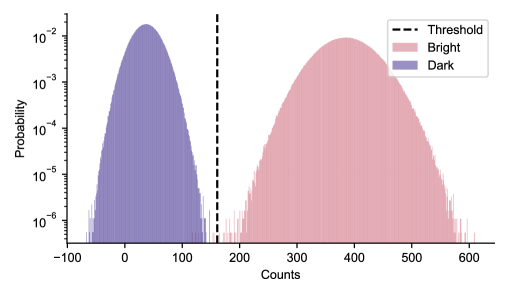
To determine the detection discrimination threshold, we first perform a series of population detection pulses with a single ion in the trap prepared in the level and record the resulting counts. The results from these population detections should all be bright. We then perform the same number of population detection pulses, but this time turning off the laser. In this case, the population will get shelved in the metastable level, and the outcomes of the population detection are expected to be dark.
The threshold for discriminating between bright and dark is then set by fitting Gaussian functions to the bright and dark distributions and minimizing the overlap between the two fitted curves, as discussed in Ref. [43]. An example of such a calibration is shown in Fig. S7.
S4.1.3 Optical detection error
The optical detection error is the error associated with an ion that fluoresces during population detection (i.e. is within the manifold) being measured as dark, an ion that doesn’t fluoresce during population detection (i.e. an ion that starts and remains within the population detection pulse, or equivalently, the lack of an ion) being recorded as bright. This error can be decreased by increasing the signal generated by a fluorescing ion or, equivalently, by increasing the efficiency of the imaging system used to collect light from the ions and/or the camera exposure time. In this section, we evaluate the quality of this discrimination independently of the decay of the metastable level. We will call the probability to classify an ion in the level as bright and the probability to classify an ion in the level (that remained in the level during the population detection pulse) to be dark as .
To evaluate the error of a bright outcome, i.e. , we initialize the ion into via optical pumping and then perform three consecutive population detection pulses. The error of a bright outcome is given by the probability of a dark result in the second pulse, provided the first and third pulses result in a bright outcome. We repeat this experiment times to accumulate sufficient statistics.
To evaluate the error of a dark outcome, i.e. , we initialize the ion into the state and then transfer the population to . We perform three consecutive population detection pulses. The error of a dark outcome is given by the probability of a bright result after the second pulse provided the first and third pulses result in a bright outcome. By demanding that the first and third pulses result in a dark outcome, we are able to decouple the error due to decay of the metastable level (see section S4.2) from the optical detection error.We repeat this experiment times to accumulate sufficient statistics.
The results from these experiments are shown in Fig. S8. We find a bright state error of and a dark state error of . The slight difference in bright and dark errors is caused by the non-gaussian tail of the bright count distribution (we did not investigate its origin).
S4.2 Metastable level decay probability
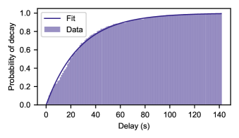
After the ion is prepared in , it decays into with probability , where is the time after preparation and is the lifetime of the state. To measure , we first optically pump the ion into and then map it to followed by a population detection pulse to confirm successful preparation into the metastable level. We then continuously measure the photon count rate from the ion. Once a bright measurement is obtained, the duration for which the ion was dark is recorded, and the procedure is repeated. The results from this experiment are shown in Fig. S9. We observe a lifetime of . This is slightly lower than the natural lifetime of the level in of [58]. We believe this is limited by leakage of the laser light used to drive the transition.
We now calculate the probability that an ion originally encoded in the level is measured as bright in our protocol due to decay, assuming perfect optical detection. This is only relevant for the population detection step used to infer the quantum measurement result. A decay during any of the remaining population detection steps may lead to unnecessarily flagged shots but not an error in the final measurement result.
Let’s assume that for a given population detection pulse of length , if the ion decays within some time from the start of the pulse, the result would be a bright measurement. However, if the ion decays during the last of the pulse, the result would still be a dark measurement, since it did not spend enough time in the level to be recorded as bright. Now consider the measurement sequence as in Fig. 1(b), with followed by . Assume further that the population transfer step is much shorter than the population detection step, such that and can be considered as occurring in immediate succession. This is a good approximation in our experiment since the average duration of the population transfer pulses is , compared to the total detection pulse duration of . In this case, if an ion in decays during time from the start of , the outcome of is bright, so an error flag is raised. Hence, the only way a SPAM error can occur (i.e. the outcome of is bright) without raising an error flag is if the decay occurs during the last of , or during the first of . Thus, the relevant timescale for decay is . Based on the lifetime measurement above, we thus expect a dark ion to be measured as bright during with probability .
S4.3 Total population detection error and SPAM protocol error
The total error for a single population detection can be calculated by combining the optical detection error and the metastable decay probability during the detection pulse. The error for an ion that was prepared into a bright state is then given by the bright state optical detection error i.e. . Conversely, the error in the readout of an ion that was prepared into the dark state is given by . The average population detection error for the two input states is then .
S5 SPAM success probability
The protocol presented in this paper effectively eliminates errors acquired during standard SPAM procedures at the expense of a reduced success probability. This success probability is determined by the errors in the operations in all steps of the protocol, such as optical pumping and the population transfer pulses. The measured error probabilities for each of these processes are shown in Table 1.
In what follows, we calculate the expected fraction of rejected shots at each of the protocol steps. The model includes optical pumping errors and population transfer errors, as well as qubit decay, but ignores the optical readout errors, which are orders of magnitude smaller. The calculated results are shown in able 2 and compared with experimental observations. We find that many of the measured values agree well with calculations, and we attribute any differences to system drifts throughout the measurement period.
| Error type | Error |
|---|---|
| Optical pumping | |
| Qubit type | State | Shots rejected | Expected shots rejected |
|---|---|---|---|
| O | |||
| O | |||
| M | |||
| M | |||
| G | |||
| G |
S6 Observable statistics
In our SPAM protocol, the probability of discarding a shot depends in general on the qubit state. As a result, when averaging over multiple experimental shots, incorrect probabilities may be assigned to different measurement outcomes. In this section, we quantify this effect, perform validation experiments, and describe the mitigation strategies.
Consider the problem of measuring the observable . We can estimate its value using the formula , where and are the probabilities that the measurements projects the input state into and respectively. In the experiment, we associate those with bright () and dark () outcomes of respectively, i.e. ideally and , such that .
However, after post-selection, the apparent observable average measured in the experiment is given by , where the probabilities are now conditional on the shot being accepted, which we denote as . Because the probability for accepting the input state can differ from the probability for accepting the input state , it is possible that , leading to a bias in the observable measurement.
We can write the probability to measure a bright outcome as
| (S1) |
where denotes the qubit state after an ideal projective measurement. Using we can calculate:
| (S2) |
One method to correct the bias is to measure by preparing each qubit state independently, and then extract the unbiased results from experimental results using the equations above.
Using conditional probability, we can write . This highlights the two error sources that may bias the observable measured. characterizes the single shot accuracy of the implementation of the protocol. In the ideal case this is and , but in our system, decay error reduces the latter by , see Sec. S4. On the other hand, , characterizes the probability of a shot measuring state to be accepted. In our system, imperfect population transfer between and creates population transfer errors at the level of , as characterized in Section S5.
Considering the decay error to be negligible compared to the error from population transfer pulses, we can simplify the equations above to read
| (S3) |
The apparent observable is then given by
| (S4) |
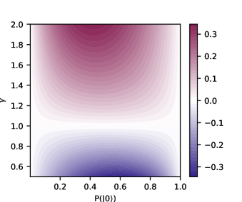
where . If , we recover . In fig. S10, we use Eq. S4 to plot the bias for and .
We experimentally measure the observable bias as follows. We start by preparing into or as outlined in Fig. 1 in the main text. Next, we perform a rotation to produce an equal superposition state of and , where we expect . The qubit state is then measured as in Fig. 1 in the main text. We change the duration of individual population transfer pulses between and from its pre-calibrated value of to simulate an error in the pulses. The measurement outcome is then calculated and plotted in Fig. S11. In the same graph, we also plot the expected functional form of the bias based in Eq. S4 and the expected dependence of and as tabulated in Tab. 3. We find that the measured bias closely matches the model, indicating that data post-processing using Eq. S4 can be used to eliminate bias in observable measurements.
| Name | ||
|---|---|---|
| Optical | 1 | |
| Optical | 1 | |
| Metastable | 1 | |
| Ground | 1 |