Enhancing Preference-based Linear Bandits
via Human Response Time

Abstract

Binary human choice feedback is widely used in interactive preference learning for its simplicity, but it provides limited information about preference strength. To overcome this limitation, we leverage human response times, which inversely correlate with preference strength, as complementary information. Our work integrates the EZ-diffusion model, which jointly models human choices and response times, into preference-based linear bandits. We introduce a computationally efficient utility estimator that reformulates the utility estimation problem using both choices and response times as a linear regression problem. Theoretical and empirical comparisons with traditional choice-only estimators reveal that for queries with strong preferences (“easy” queries), choices alone provide limited information, while response times offer valuable complementary information about preference strength. As a result, incorporating response times makes easy queries more useful. We demonstrate this advantage in the fixed-budget best-arm identification problem, with simulations based on three real-world datasets, consistently showing accelerated learning when response times are incorporated.

1 Introduction

Interactive preference learning from human binary choices is crucial in many systems and applications, including recommendation systems [31, 57, 10, 20], assistive robots [55, 66], assortment optimization [54, 1], and fine-tuning large language models [60, 43, 46, 47, 6]. This form of human feedback is widely adopted for its simplicity and minimal cognitive load on users [75, 73, 36]. Preference learning from binary choices is typically modeled as a preference-based bandit problem [8, 30], where a system queries users with pairs of options and refines its understanding of their preferences. However, while choices help estimate preferences, they provide limited information on preference strength [78]. To address this limitation, researchers have incorporated additional explicit feedback mechanisms, such as ratings [59, 50], labels [75], and slider bars [73, 6], but these approaches often increase interface complexity and the cognitive burden on users [35, 36].

In this paper, we propose leveraging an implicit form of human feedback—response time—to provide additional information about preference strength. Unlike explicit feedback, response time is typically effortless and unobtrusive to measure [16] and provides valuable complementary information beyond what choices alone can offer [15, 3]. For instance, consider an online retailer that repeatedly presents users with two options: purchase or skip a recommended product [34]. Most users skip products most of the time [32], resulting in a probability of skipping close to $1$ across most products. As a result, the choices themselves don’t convey how strongly a product is liked or disliked, making it difficult for the retailer to identify the user’s preferences. In such cases, response time provides a useful solution. Psychological research has shown an inverse relationship between response time and preference strength [16]: users who strongly prefer to skip a product do so quickly, while longer response times may indicate weaker preferences. Thus, even when choices seem similar, response time can reveal subtle differences in preference strength.

Despite its potential, leveraging response time for preference learning presents significant challenges. Psychological research has extensively studied the relationship between human choices and response times [16, 18] through complex models like Drift-Diffusion Models [51, 38] and Race Models [67, 12]. While these models provide valuable insights into human behavior and align with neurobiological evidence [71], they rely on computationally intensive parameter estimation methods [52, 39, 3], such as hierarchical Bayesian inference [72] and maximum likelihood estimation (MLE) [38], making them unsuitable for real-time interactive systems. Although faster estimators exist [68, 69, 29, 26, 9], they are typically designed for parameter estimation for a single pair of options and do not aggregate data across multiple pairs. This limits their ability to leverage structures like linear utility functions, which are essential in preference learning with large option spaces [40, 55, 22, 57, 20], and cognitive models for human multi-attribute decision-making [65, 24, 77].

To overcome these limitations, we adopt the difference-based EZ diffusion model [68, 9] with linear human utility functions and propose a computationally efficient utility estimator that incorporates both choices and response times. By leveraging the relationship among human utilities, choices, and response times, our estimator reformulates the estimation as a linear regression problem. This reformulation allows our estimator to aggregate information from all available pairs and be compatible with standard linear bandit algorithms [4] for interactive learning. We compared our estimator to the traditional method, which relies solely on choices and logistic regression [4, 30]. Our theoretical and empirical analyses show that for queries with strong preferences (“easy” queries), choices alone provide limited information, while response times offer valuable additional insights into preference strength. Hence, incorporating response times makes easy queries more useful.

We applied our estimator to investigate the benefits of incorporating response times in the fixed-budget best-arm identification problem [27, 33] within preference-based bandits with linear human utility functions [4, 30]. We integrated two versions of the Generalized Successive Elimination algorithm [4]: one using both choices and response times, and the other relying on choices alone. Through simulations based on three real-world datasets of human choices and response times [58, 15, 38], we consistently observed that incorporating response times significantly enhanced performance, validating our earlier example of the online retailer. To the best of our knowledge, this is the first work to integrate response times into the framework of bandit and RL.

Section 2 introduces the preference-based linear bandit problem and the difference-based EZ diffusion model. Section 3 presents our estimator, which incorporates both choices and response times, and compares it theoretically to the choice-only estimator. Section 4 integrates both estimators into the Generalized Successive Elimination algorithm. Section 5 presents empirical results for estimation and bandit learning. Section 6 discusses the limitations of our approach. Appendix B reviews response time models, parameter estimators, and their connection to preference-based RL.

Nomenclature: We use $[n]$ to denote the set $\{1,\dots,n\}$. For a scalar random variable $x$, $\mathbb{E}\left[x\right]$ and $\mathbb{V}\left[x\right]$ denote its expectation and variance, respectively. The notation $\text{sgn}(x)$ refers to the sign of $x$.

2 Problem setting and preliminaries

We consider preference-based bandits with a linear utility function [30], extending both dueling bandits [79] and logistic bandits [4]. The learner is given a finite set of options (referred to as “arms”), each represented by a feature vector in $\mathcal{Z}\subset\mathbb{R}^{d}$, and a finite set of binary comparison queries, where the features are the differences between pairs of arms, denoted by $\mathcal{X}\subset\mathbb{R}^{d}$. For instance, if the learner can query any pair of arms, the query set is $\mathcal{X}=\left\{z-z^{\prime}\colon z,z^{\prime}\in\mathcal{Z}\right\}$. In the online retailer scenario from section 1, the query set becomes $\mathcal{X}=\left\{z-z_{\text{skip}}\colon z\in\mathcal{Z}\right\}$, where $z$ represents the option to purchase a product and $z_{\text{skip}}$ represents the option to skip (often set to $\mathbf{0}$). For each arm $z\in\mathcal{Z}$, the human utility is defined as $u_{z}\coloneqq z^{\top}\theta^{*}$, where $\theta^{*}\in\mathbb{R}^{d}$ represents the parameters of human preference. For any query $x\in\mathcal{X}$, the utility difference is then defined as $u_{x}\coloneqq x^{\top}\theta^{*}$.

Given a query $x\coloneqq z_{1}-z_{2}\in\mathcal{X}$, we model human choices and response times using the difference-based EZ-Diffusion Model (dEZDM) [68, 9], integrated with a linear utility structure. (For a detailed comparison with other models, see section B.1.) This model views human choice-making as a stochastic evidence accumulation process for comparing the two options. As shown in fig. 1(a), upon receiving a query $x$, the human first spends a fixed amount of non-decision time, denoted by $t_{\text{nondec}}>0$, to perceive and encode the query. Then, evidence $E_{x}$ accumulates over time according to a Brownian motion with drift $x^{\top}\theta^{*}$ and two symmetric absorbing barriers, $a>0$ and $-a$. Specifically, at time $t_{\text{nondec}}+\tau$ where $\tau\geq 0$, the evidence $E_{x,\tau}=x^{\top}\theta^{*}\cdot\tau+B(\tau)$, where $B(\tau)\sim\mathcal{N}(0,\tau)$ is standard Brownian motion. This process continues until the evidence reaches either the barrier $a$ or $-a$, at which point a decision is made. The random stopping time, $t_{x}\coloneqq\min\left\{\tau>0\colon E_{x,\tau}\in\left\{a,-a\right\}\right\}$, represents the decision time. If $E_{x,t_{x}}=a$, the human chooses $z_{1}$; if $E_{x,t_{x}}=-a$, they choose $z_{2}$. The choice outcome is denoted by the random variable $c_{x}$, where $c_{x}=1$ if $z_{1}$ is chosen, and $-1$ if $z_{2}$ is chosen. The total response time, $t_{\text{RT},x}$, is the sum of the non-decision time and the decision time: $t_{\text{RT},x}=t_{\text{nondec}}+t_{x}$. The choice probability, choice expectation, and decision time expectation are as follows [48, eq. (A.16) and (A.17)]:

$$\forall x\in\mathcal{X}\colon \mathbb{P}\left[c_{x}=1\right]=\frac{1}{1+\exp(-2ax^{\top}\theta^{*})},\quad\mathbb{E}\left[c_{x}\right]=\tanh(ax^{\top}\theta^{*}),$$ (1)

$$\mathbb{E}\left[t_{x}\right]=\begin{cases}\frac{a}{x^{\top}\theta^{*}}\tanh(ax^{\top}\theta^{*})\quad\text{if }x^{\top}\theta^{*}\neq 0\\ a^{2}\hfill\text{ if }x^{\top}\theta^{*}=0\end{cases}.$$ (2)

Figures 1(b) and 1(c) illustrate the roles of the parameters $x^{\top}\theta^{*}$ and $a$. First, the absolute drift (or the absolute utility difference), $|x^{\top}\theta^{*}|$, represents the easiness of the query [39]. High $|x^{\top}\theta^{*}|$ indicates an easy query, resulting in short response times and consistent choices. Conversely, when $|x^{\top}\theta^{*}|$ is low (near $0$), the query is difficult, leading to long response times and inconsistent choices. Second, the barrier $a$ reflects the human’s conservativeness in decision-making [39]. A higher $a$ means more evidence is required to make a decision, resulting in longer response times and more consistent choices. Lower $a$ leads to quicker decisions and less consistent choices.

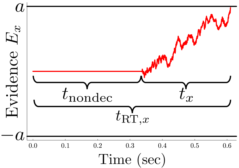
(a)

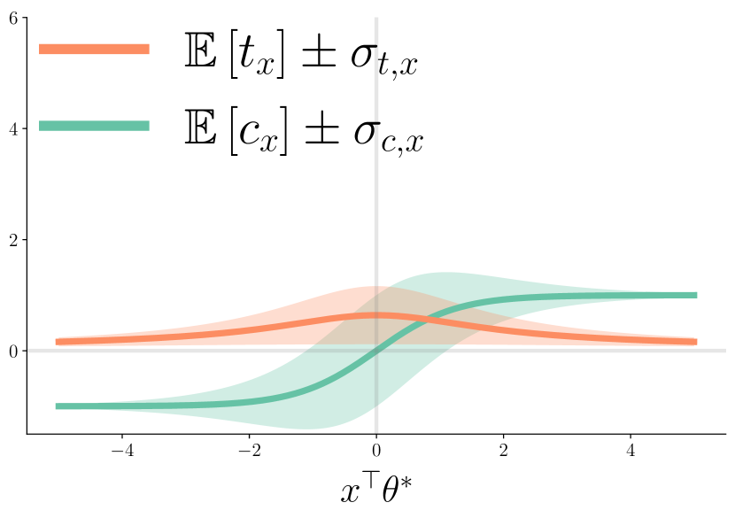
(b) $a=0.8$

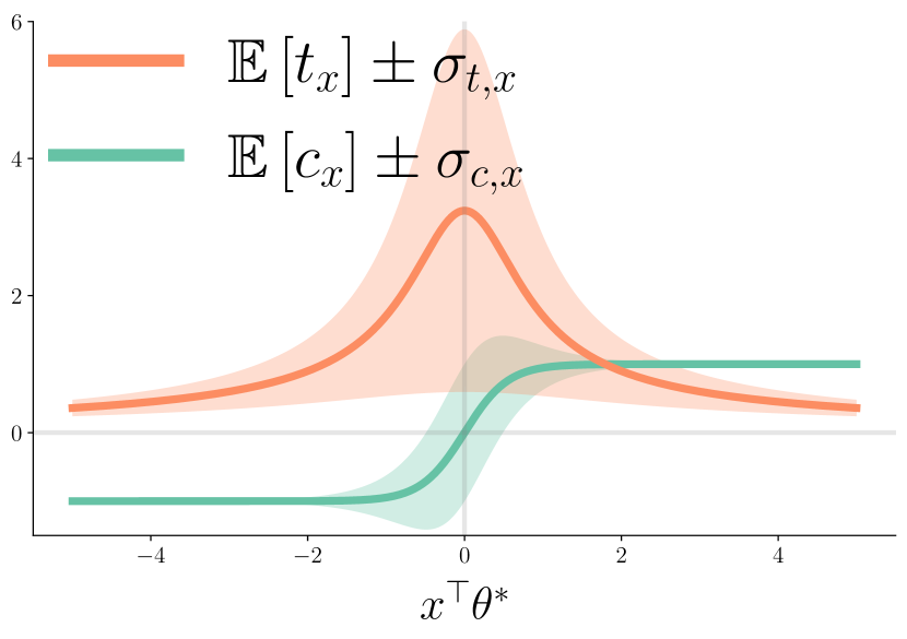
(c) $a=1.8$

Figure 1: (a) illustrates the evidence accumulation process. For a query $x\in\mathcal{X}$, the human first spends a fixed non-decision time $t_{\text{nondec}}$ encoding the query. Then, the evidence accumulates according to a Brownian motion with drift $x^{\top}\theta^{*}$ till it reaches either the barrier $a>0$ or $-a$. The random stopping time is the decision time $t_{x}$ and the total response time $t_{\text{RT},x}=t_{\text{nondec}}+t_{x}$. (b) and (c) illustrates the expected choice $\mathbb{E}[c_{x}]$ and the expected decision time $\mathbb{E}[t_{x}]$, with shaded bands representing $1$ standard deviation, as functions of the utility difference $x^{\top}\theta^{*}$ for two different values of the barrier $a$.

We adopt the common assumption that $t_{\text{nondec}}$ is constant across all queries for a single human [16, 77] and further assume that $t_{\text{nondec}}$ is known to the learner. This allows the learner to perfectly recover $t_{x}$ from the observed $t_{\text{RT},x}$. In section 5.2, we empirically show that even when $t_{\text{nondec}}$ is unknown, its impact on the performance of our method incorporating response times is minimal.

Learning objective: Best-arm identification with a fixed budget

This paper addresses the fixed-budget best-arm identification problem [27, 33]. The learner is given a total interaction time budget $B>0$, an arm set $\mathcal{Z}$, a query set $\mathcal{X}$, and a non-decision time $t_{\text{nondec}}$. The human’s preference vector $\theta^{*}$ and the barrier $a$ are unknown. In each episode $s\in\mathbb{N}$, the learner samples a query $x_{s}\in\mathcal{X}$ and observes the human feedback $(c_{x_{s},s},t_{x_{s},s})$ generated by the dEZDM. This episode consumes $t_{\text{RT},x_{s},s}$ time. When the budget is exhausted at some episode $S$, i.e., $\sum_{s=1}^{S}t_{\text{RT},x_{s},s}>B$, the interaction terminates and the learner recommends an arm $\widehat{z}\in\mathcal{Z}$. The learner’s goal is to recommend the unique best arm $z^{*}\coloneqq\operatorname*{arg\,max}_{z\in\mathcal{Z}}z^{\top}\theta^{*}$, minimizing the error probability $\mathbb{P}\left[\widehat{z}\neq z^{*}\right]$.

To solve this problem, we use the Generalized Successive Elimination (GSE) algorithm [4, 2, 76] for sequential querying and arm recommendation. The GSE algorithm divides the budget $B$ evenly into multiple phases. Within each phase $s$, it strategically samples queries till the allocated budget is exhausted, collects human choices and response times, computes $\widehat{\theta}_{s}$ (an estimate of $\theta^{*}$), and eliminates arms with low estimated utilities based on $\widehat{\theta}_{s}$. The effectiveness of incorporating response times depends on designing an estimator that augments choices with preference strength to improve estimation accuracy. In section 3, we detail this estimator and compare it theoretically to the traditional choice-only estimator, while section 4 presents the GSE algorithm integrated with both estimators.

3 Utility estimation

In this section, we address the problem of estimating human preference $\theta^{*}$ from a fixed dataset, denoted by $\left\{x,c_{x,s_{x,i}},t_{x,s_{x,i}}\right\}_{x\in\mathcal{X}_{\text{sample}},i\in[n_{x}]}$. Here $\mathcal{X}_{\text{sample}}$ denotes the set of queries contained in the dataset, $n_{x}$ denotes the number of samples for the query $x\in\mathcal{X}_{\text{sample}}$, and $s_{x,i}$ denotes the episode where we sample $x$ for the $i$-th time. Samples from each query $x$ are i.i.d., while samples from different queries are independent. Section 3.1 introduces a new estimator, called the “choice-decision-time estimator,” which uses both choices and response times, alongside the widely used “choice-only estimator” that relies solely on choices [4, 30]. Sections 3.2 and 3.3 provide a theoretical comparison of the two estimators, examining both their asymptotic and non-asymptotic performance, respectively, and highlighting the benefits of incorporating response times. Later, section 5.1 provides empirical comparisons, confirming our theoretical analysis.

3.1 Choice-decision-time estimator vs. choice-only estimator

The choice-decision-time estimator is based on the following relationship between human utilities, choices, and response times, derived from eqs. 1 and 2:

$$\forall x\in\mathcal{X}\colon x^{\top}\frac{\theta^{*}}{a}=\frac{\mathbb{E}\left[c_{x}\right]}{\mathbb{E}\left[t_{x}\right]},$$ (3)

Intuitively, if a human facing query $x$ provides consistent choices (i.e., large $|\mathbb{E}[c_{x}]|$) and makes decisions quickly (i.e., small $\mathbb{E}[t_{x}]$), the query is easy, indicating a strong preference (i.e., large $|x^{\top}\theta^{*}|$). This identity reframes the estimation of $\theta^{*}$ as a linear regression problem. Accordingly, the choice-decision-time estimator computes the empirical means for both choices and response times, aggregates the ratios across all sampled queries, and applies ordinary least squares (OLS) to estimate $\theta^{*}/a$. Since the ranking of arm utilities based on $\theta^{*}/a$ matches that based on $\theta^{*}$, estimating $\theta^{*}/a$ is sufficient for identifying the best arm. This estimate, denoted by $\widehat{\theta}_{\text{CH,DT}}$, is formally calculated as:

$$\widehat{\theta}_{\text{CH,DT}}\coloneqq\left(\sum_{x\in\mathcal{X}_{\text{sample}}}n_{x}\>xx^{\top}\right)^{-1}\sum_{x\in\mathcal{X}_{\text{sample}}}n_{x}\>x\>\>\frac{\sum_{i=1}^{n_{x}}c_{x,s_{x,i}}}{\sum_{i=1}^{n_{x}}t_{x,s_{x,i}}}.$$ (4)

In contrast, the choice-only estimator is based on eq. 1, which shows that for each query $x\in\mathcal{X}$, the random variable $(c_{x}+1)/2$ follows a Bernoulli distribution with mean $1/[1+\exp(-x^{\top}\cdot 2a\theta^{*})]$. Similar to the choice-decision-time estimator, the parameter $2a$ does not affect the ranking of the arms, so identifying $2a\theta^{*}$ is sufficient for best-arm identification. Estimating $2a\theta^{*}$ becomes a logistic regression problem [4, 30], which can be solved using the following MLE:

$$\widehat{\theta}_{\text{CH}}\coloneqq\operatorname*{arg\,max}_{\theta\in\mathbb{R}^{d}}\sum_{x\in\mathcal{X}_{\text{sample}}}\sum_{i=1}^{n_{x}}\log\mu(c_{x,s_{x,i}}\>x^{\top}\theta),$$ (5)

where $\mu(y)\coloneqq 1/[1+\exp(-y)]$ is the standard logistic function. This MLE lacks a closed-form solution but can be efficiently solved in practice using methods such as Newton’s algorithm [44, 23].

3.2 Asymptotic normality of the two estimators

The choice-decision-time estimator from eq. 4 satisfies the following asymptotic normality result, as proven in section C.2:

Theorem 3.1 (Asymptotic normality of $\widehat{\theta}_{\text{CH,DT}}$).

Suppose the learner has an i.i.d. dataset $\left\{x,c_{x,s_{x,i}},t_{x,s_{x,i}}\right\}_{i\in[n]}$ for every $x\in\mathcal{X}_{\text{sample}}$, where $\sum_{x\in\mathcal{X}_{\text{sample}}}xx^{\top}\succ 0$, and the datasets for different $x\in\mathcal{X}_{\text{sample}}$ are independent. Then, for any $y\in\mathbb{R}^{d}$, as $n\to\infty$, the following holds:

$$\sqrt{n}\>y^{\top}\left(\widehat{\theta}_{\text{CH,DT},n}-\theta^{*}/a\right)\overset{D}{\longrightarrow}\mathcal{N}(0,\zeta^{2}/a^{2}).$$

Here, the asymptotic variance $\zeta^{2}$ is a problem-specific constant that is upper bounded as follows:

$$\zeta^{2}\leq\left\|y\right\|^{2}_{\left(\sum_{x\in\mathcal{X}_{\text{sample}}}\mathcal{M}_{\text{CH,DT}}^{\text{asym}}\cdot xx^{\top}\right)^{-1}},$$

$$\text{where}\,\,\mathcal{M}_{\text{CH,DT}}^{\text{asym}}\coloneqq\min_{x\in\mathcal{X}_{\text{sample}}}m_{\text{CH,DT}}^{\text{asym}}(x^{\top}\theta^{*})\,\,\,\,\,\,\text{and}\,\,\,\,\,\,m_{\text{CH,DT}}^{\text{asym}}(x^{\top}\theta^{*})\coloneqq\frac{1}{\frac{a^{2}}{\mathbb{E}\left[t_{x}\right]^{2}}\mathbb{V}\left[c_{x}\right]+\frac{a^{2}\mathbb{E}\left[c_{x}\right]^{2}}{\mathbb{E}\left[t_{x}\right]^{4}}\mathbb{V}\left[t_{x}\right]}.$$

The constants $\mathbb{E}\left[t_{x}\right]$, $\mathbb{E}\left[c_{x}\right]$, $\mathbb{V}\left[c_{x}\right]$, and $\mathbb{V}\left[t_{x}\right]$ are detailed in section C.1 and depend only on the utility difference $x^{\top}\theta^{*}$ for any fixed barrier $a$. In this asymptotic variance upper bound, each sampled query is weighted by the common factor $\min_{x}m_{\text{CH,DT}}^{\text{asym}}\left(x^{\top}\theta^{*}\right)$. Intuitively, the true human utilities are not observed directly but are inferred through the signals provided by choices and response times. This weight represents how much information from each query $x$ is preserved in these signals. Larger weights indicate more retained information, resulting in lower variance and more accurate estimation.

In contrast, the choice-only estimator from eq. 5 has the following asymptotic normality result as described in Gourieroux and Monfort [28, proposition 4] and McFadden [42, theorem 3]:

Theorem 3.2 (Asymptotic normality of $\widehat{\theta}_{\text{CH}}$).

Suppose the learner has an i.i.d. dataset $\left\{x,c_{x,s_{x,i}},t_{x,s_{x,i}}\right\}_{i\in[n]}$ for every $x\in\mathcal{X}_{\text{sample}}$, where $\sum_{x\in\mathcal{X}_{\text{sample}}}xx^{\top}\succ 0$, and the datasets for different $x\in\mathcal{X}_{\text{sample}}$ are independent. Then, for any $y\in\mathbb{R}^{d}$, as $n\to\infty$, the following holds:

$$\sqrt{n}y^{\top}\left(\widehat{\theta}_{\text{CH},n}-2a\theta^{*}\right)\overset{D}{\longrightarrow}\mathcal{N}\left(0,4a^{2}\left\|y\right\|^{2}_{\left(\sum_{x\in\mathcal{X}_{\text{sample}}}m_{\text{CH}}^{\text{asym}}(x^{\top}\theta^{*})xx^{\top}\right)^{-1}}\right),$$

where $m_{\text{CH}}^{\text{asym}}(x^{\top}\theta^{*})\coloneqq 4a^{2}\;\dot{\mu}(2ax^{\top}\theta^{*})$.

Here, $\dot{\mu}(\cdot)$ denotes the first-order derivative of the function $\mu(\cdot)$ defined in eq. 5. In this asymptotic variance, each sampled query $x$ is weighted by its own factor $m_{\text{CH}}^{\text{asym}}(x^{\top}\theta^{*})$, which represents the amount of information from each query $x$ that is preserved in the choice signals.

The weights in theorems 3.1 and 3.2 highlight how choice and response time signals retain different amounts of information about human preferences. The choice-decision-time estimator applies a single “min-weight” across all queries, denoted by $\min_{x}m_{\text{CH,DT}}^{\text{asym}}(x^{\top}\theta^{*})$, with $m_{\text{CH,DT}}^{\text{asym}}(\cdot)$ illustrated by the orange curves in fig. 2(a). In contrast, the choice-only estimator assigns each query $x$ its own weight, $m_{\text{CH}}^{\text{asym}}(x^{\top}\theta^{*})$, shown as the gray curves in fig. 2(a). As illustrated, first, as the query becomes harder—when the utility difference $x^{\top}\theta^{*}$ approaches $0$—both $m_{\text{CH,DT}}^{\text{asym}}(x^{\top}\theta^{*})$ and $m_{\text{CH}}^{\text{asym}}(x^{\top}\theta^{*})$ increase, indicating that harder queries carry more information than easier ones. Second, as the barrier $a$ increases from $0.5$ to $1.5$, the orange curve, representing $m_{\text{CH,DT}}^{\text{asym}}(\cdot)$, rises across all queries, regardless of utility difference. This leads to a lower asymptotic variance upper bound and improved estimation. Intuitively, a larger barrier suggests more conservative human decision-making, resulting in longer response times and more consistent choices, which provide stronger signals for estimation. By contrast, as $a$ increases, the gray curve, representing $m_{\text{CH}}^{\text{asym}}(\cdot)$, rises for hard queries but falls for easy ones. This indicates that the choice-only estimator gathers more information from hard queries but less from easy queries as the human becomes more conservative.

Finally, comparing the weights of the two estimators reveals our key insight. As shown in fig. 2(a), the orange curves, representing $m_{\text{CH,DT}}^{\text{asym}}(\cdot)$, are consistently higher than the gray curves, representing $m_{\text{CH}}^{\text{asym}}(\cdot)$. However, the choice-decision-time estimator’s min-weight, $\min_{x}m_{\text{CH,DT}}^{\text{asym}}(\cdot)$, can be either larger or smaller than the choice-only estimator’s weights, $m_{\text{CH}}^{\text{asym}}(\cdot)$, depending on the query set. For instance, when the barrier $a$ is small (e.g., $a=0.5$), the choice-decision-time estimator’s min-weight is likely smaller than the choice-only estimator’s weights, suggesting that in this case, incorporating response times may not improve performance. On the other hand, when $a$ is large (e.g., $a=1.5$) and the queries are easy, the choice-only estimator’s weights shrink significantly, while the choice-decision-time estimator’s min-weight remains relatively large. This demonstrates that incorporating response times makes easy queries more useful, resulting in improved estimation performance.

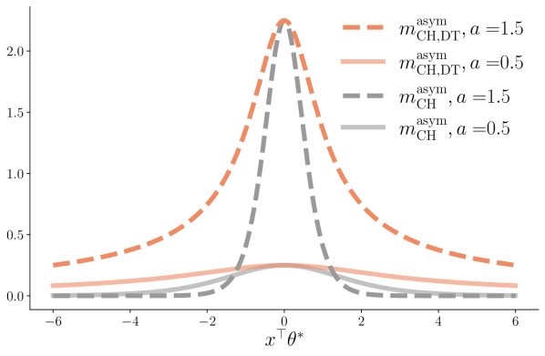
(a) Weights in the asymptotic variances

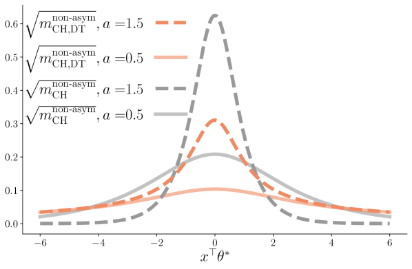
(b) Weights in the non-asymptotic concentrations

Figure 2: (a) compares the weights in the asymptotic variances for the choice-decision-time estimator (theorem 3.1) and the choice-only estimator (theorem 3.2) as a function of utility difference $x^{\top}\theta^{*}$, for two different values of the barrier $a$. (b) compares the weights in the non-asymptotic concentration bounds for both estimators (theorems 3.3 and 3.4) as a function of $x^{\top}\theta^{*}$, for two values of $a$.

3.3 Non-asymptotic concentration of the two estimators for utility difference estimation

In this section, we consider the simplified problem of estimating the utility difference for a single query, without aggregating data from multiple queries. Comparing the non-asymptotic concentration bounds of both estimators in this scenario provides insights similar to those discussed in section 3.2. A non-asymptotic analysis for estimating the human preference vector $\theta^{*}$ is left for future work.

Given a query $x\in\mathcal{X}$, the simplified problem focuses on estimating its utility difference $u_{x}\coloneqq x^{\top}\theta^{*}$ using the i.i.d. dataset $\{(c_{x,s_{x,i}},t_{x,s_{x,i}})\}_{i\in[n_{x}]}$. Applying the choice-decision-time estimator from eq. 4 yields the following estimate (for details, see section C.3.1):

$$\widehat{u}_{x,\text{CH,DT}}\coloneqq\frac{\sum_{i=1}^{n_{x}}c_{x,s_{x,i}}}{\sum_{i=1}^{n_{x}}t_{x,s_{x,i}}}.$$ (6)

In contrast, applying the choice-only estimator from eq. 5 yields the following estimate (for details, see section C.3.2):

$$\widehat{u}_{x,\text{CH}}\coloneqq\mu^{-1}\left(\frac{1}{n_{x}}\sum_{i=1}^{n_{x}}\frac{c_{x,s_{x,i}}+1}{2}\right),$$ (7)

where $(c_{x,s_{x,i}}+1)/2$ is the one-zero-coded binary choice and $\mu^{-1}(p)\coloneqq\log\left(p/(1-p)\right)$ is the logit function, the inverse of $\mu$ introduced in eq. 5. As with the estimators in section 3.1, the choice-decision-time estimator in eq. 6 estimates $u_{x}/a$, while the choice-only estimator in eq. 7 estimates $2au_{x}$. Interestingly, the choice-only estimator in eq. 7 aligns with the drift estimator for the EZ-diffusion model, as proposed in Wagenmakers et al. [68, eq. (5)]. Additionally, the estimators in Xiang Chiong et al. [74, eq. (6)] and Berlinghieri et al. [9, eq. (7)] can be viewed as combinations of the two estimators presented in eqs. 6 and 7. In section 5, we apply Wagenmakers et al. [68, eq. (5)] and Xiang Chiong et al. [74, eq. (6)] to the full bandit problem and empirically demonstrate that they are outperformed by our estimator proposed in eq. 4.

Assuming the utility difference is nonzero, the choice-decision-time estimator in eq. 6, has the following non-asymptotic concentration result, proved in section C.3.1:

Theorem 3.3 (Non-asymptotic concentration of $\widehat{u}_{x,\text{CH,DT}}$).

For each query $x\in\mathcal{X}$ with $u_{x}\neq 0$, suppose that the learner has an i.i.d. dataset $\left\{\left(c_{x,s_{x,i}},t_{x,s_{x,i}}\right)\right\}_{i\in[n_{x}]}$. Then, for any $\epsilon>0$ satisfying $\epsilon\leq\min\left\{|u_{x}|/(\sqrt{2}a),\left(1+\sqrt{2}\right)a|u_{x}|/\mathbb{E}\left[t_{x}\right]\right\}$, we have the following:

$$\begin{split}\mathbb{P}\left(\left|\widehat{u}_{x,\text{CH,DT}}-\frac{u_{x}}{a}\right|>\epsilon\right)\leq 4\exp\left(-m_{\text{CH,DT}}^{\text{non-asym}}\left(x^{\top}\theta^{*}\right)\cdot n_{x}\left[\epsilon\cdot a\right]^{2}\right),\end{split}$$

where $m_{\text{CH,DT}}^{\text{non-asym}}\left(x^{\top}\theta^{*}\right)\coloneqq\mathbb{E}\left[t_{x}\right]^{2}\ /\ \left[(2+2\sqrt{2})^{2}\ a^{2}\right]$.

In contrast, the choice-only estimator in eq. 7 has the following non-asymptotic concentration result, which can be directly adapted from Jun et al. [30, theorem 1]:

Theorem 3.4 (Non-asymptotic concentration of $\widehat{u}_{x,\text{CH}}$).

For each query $x\in\mathcal{X}$, suppose that the learner has an i.i.d. dataset $\left\{c_{x,s_{x,i}}\right\}_{i\in[n_{x}]}$. Then, for any positive $\epsilon<\sqrt{1/12}$, if $n_{x}\geq 1/\dot{\mu}(2au_{x})\cdot\max\{2.4^{2}\log(6e)/\epsilon^{2},64\log(3)/(1-12\epsilon^{2})\}$, we have the following:

$$\begin{split}\mathbb{P}\left(\left|\widehat{u}_{x,\text{CH}}-2au_{x}\right|>\epsilon\right)\leq 6\exp\left(-m_{\text{CH}}^{\text{non-asym}}\left(x^{\top}\theta^{*}\right)\cdot n_{x}\left[\epsilon/(2a)\right]^{2}\right),\end{split}$$

where $m_{\text{CH}}^{\text{non-asym}}\left(x^{\top}\theta^{*}\right)\coloneqq 4a^{2}\ \dot{\mu}(2ax^{\top}\theta^{*})\ /\ 2.4^{2}$.

The weights $m_{\text{CH,DT}}^{\text{non-asym}}(\cdot)$ and $m_{\text{CH}}^{\text{non-asym}}(\cdot)$, presented in theorems 3.3 and 3.4, respectively, determine how fast the estimation error decays as the number of data points $n_{x}$ increases—larger weights result in better estimates. Although these weights may not be optimal due to the proof technique, they still convey key insights, similar to those discussed in section 3.2. To illustrate these insights, we plot the square roots of the weights in fig. 2(b). First, for a fixed barrier $a$, as the query $x$ becomes harder, both $m_{\text{CH,DT}}^{\text{non-asym}}(x^{\top}\theta^{*})$ and $m_{\text{CH}}^{\text{nonasym}}(x^{\top}\theta^{*})$ increase, leading to better estimation. Second, as the barrier $a$ increases from $0.5$ to $1.5$, the orange curve, representing $m_{\text{CH,DT}}^{\text{non-asym}}(\cdot)$, do not decrease, while the gray curve, representing $m_{\text{CH}}^{\text{non-asym}}(\cdot)$, drops significantly for easy queries. This indicates that the choice-only estimator gathers more information from hard queries but less from easy ones as human decision-making becomes more conservative. Finally, comparing the weights of the two estimators reveals our key insight: the orange curves, representing $m_{\text{CH,DT}}^{\text{non-asym}}(\cdot)$, are lower than the gray curves, representing $m_{\text{CH}}^{\text{non-asym}}(\cdot)$, for hard queries, but higher for easy ones. As the barrier $a$ increases, this effect becomes even more pronounced. This confirms our insight that incorporating response times makes easy queries more useful, resulting in improved estimation performance.

Summary

Our theoretical insights from sections 3.2 and 3.3 align with the empirical findings of Clithero [15] and are further validated by our empirical results in section 5.1.

In fixed-budget best-arm identification, our choice-decision-time estimator’s ability to extract information from easy queries is crucial. A bandit learner like GSE [4] strategically samples queries, updates its estimate of $\theta^{*}$, and eliminates arms with lower utilities. Unlike the choice-only estimator, our approach extracts more information from easy queries, which also consume less time, leading to greater “bang per buck” (information per unit of resource consumption) [5]. Moreover, without knowing the true human preference $\theta^{*}$, the learner cannot know in advance which queries are hard, so cannot specifically sample them to exploit the choice-only estimator. Our estimator remains robust and effective across varying query easiness and sampling strategies. In the next section, we integrate both estimators into a bandit learning algorithm.

To illustrate the value of incorporating both choices and response times, consider this analogy: a teacher wants to identify the best student through a quiz with two-choice questions. If the questions are too easy, all students answer correctly, making it difficult to identify the top students. There are two possible solutions. First, the teacher could ask hard questions. Alternatively, the teacher could observe how quickly students complete the quiz. Even with easy questions, students who finish accurately and quickly can be identified as the best.

4 Interactive learning algorithm

In this section, we introduce the Generalized Successive Elimination (GSE) algorithm [4, 2, 76] for fixed-budget best-arm identification in preference-based linear bandits. We outline several options for each component of GSE, which will be empirically compared in section 5.

GSE’s pseudo-code is presented in algorithm 1. There is one hyper-parameter, $\eta$, that controls the number of phases, the budget per phase, and the number of arms eliminated in each phase. GSE starts by dividing the budget $B$ evenly into phases according to $\eta$ and reserves a buffer in each phase to prevent over-consuming the budget (3). In each phase, GSE first computes an experimental design, a probability distribution $\lambda$ over the query space, to determine which queries to sample during that phase. We consider two designs: the transductive design [22], $\lambda_{\text{trans}}$ (4), and the hard-query design [30], $\lambda_{\text{hard}}$ (5). Both designs minimize the worst-case variance of the estimated utility difference between surviving arms. The transductive design assigns equal weight to all queries. In contrast, the hard-query design assigns more weight to hard queries, taking advantage of the choice-only estimator’s advantage—compared to the choice-decision-time estimator—in extracting information from hard queries, as discussed in section 3.

The pseudo-code for GSE is presented in algorithm 1. The key hyper-parameter, $\eta$, controls the number of phases, the budget per phase, and the number of arms eliminated in each phase. GSE begins by dividing the budget $B$ evenly into phases based on $\eta$ while reserving a buffer in each phase to avoid over-consuming the budget (3). In each phase, GSE first computes an experimental design, represented by a probability distribution $\lambda$ over the query space, to determine which queries to sample. We consider two designs: the transductive design [22], $\lambda_{\text{trans}}$ (4), and the hard-query design [30], $\lambda_{\text{hard}}$ (5). Both designs minimize the worst-case variance of the estimated utility difference between surviving arms. The transductive design assigns equal weight to all queries. In contrast, the hard-query design assigns more weight to hard queries, taking advantage of the choice-only estimator’s advantage—compared to the choice-decision-time estimator—in extracting information from hard queries, as discussed in section 3. GSE then randomly samples queries according to the design $\lambda_{s}$ (6). Once the phase’s budget is exhausted, GSE uses the collected data to estimate $\theta^{*}$, either with the choice-and-decision-time estimator $\widehat{\theta}_{\text{CH,DT}}$ (7) or the choice-only estimator $\widehat{\theta}_{\text{CH}}$ (8). Based on these estimates, GSE eliminates arms with low utilities. This phase-by-phase elimination continues until only one arm remains in $\mathcal{Z}_{S+1}$, which GSE then recommends.

The key difference between algorithm 1 and previous GSE algorithms [4, 2, 76] is that in our problem, queries consume random response times, which are unknown to the learner beforehand. In contrast, prior work assumes each query consumes a fixed unit of resource, often using deterministic rounding methods [22, 4], rather than the sampling procedure in 6. Potentially due to this difference, our empirical study in section 5.2 suggests that the choice of $\eta$ can significantly impact bandit performance, whereas previous work typically set $\eta=2$ by default [4, section 3]. Further theoretical analysis is needed to fully understand the algorithm and determine the optimal value of $\eta$.

Algorithm 1 Generalized Successive Elimination (GSE) [4]

1:Input: arm space $\mathcal{Z}$, query space $\mathcal{X}$, non-decision time $t_{\text{nondec}}$, total budget $B$, time buffer $B_{\text{buff}}$, and elimination parameter $\eta$.

2:Initialization: $\mathcal{Z}_{1}\leftarrow\mathcal{Z}$, $s\leftarrow 1$.

3:for each phase $s=1,\dots,S\coloneqq\left\lceil\log_{\eta}|\mathcal{Z}|\right\rceil$ with the budget $B_{s}\coloneqq\frac{B}{S}-B_{\text{buff}}$ do

4:     Design 1. $\lambda_{s}\coloneqq\lambda_{\text{trans},s}\leftarrow\operatorname*{arg\,min}_{\lambda\in\blacktriangle^{|\mathcal{X}|}}\max_{z\neq z^{\prime}\in\mathcal{Z}_{s}}\|z-z^{\prime}\|^{2}_{\left(\sum_{x\in\mathcal{X}}\lambda_{x}xx^{\top}\right)^{-1}}$.

5:     Design 2. $\lambda_{s}\coloneqq\lambda_{\text{hard},s}\leftarrow\operatorname*{arg\,min}_{\lambda\in\blacktriangle^{|\mathcal{X}|}}\max_{z\neq z^{\prime}\in\mathcal{Z}_{s}}\|z-z^{\prime}\|^{2}_{\left(\sum_{x\in\mathcal{X}}\dot{\mu}(x^{\top}\widehat{\theta}_{s-1})\lambda_{x}xx^{\top}\right)^{-1}}$.

6:     Sample queries $x_{j}\sim\lambda_{s}$ and stop at $J_{s}$ if $\sum_{j=1}^{J_{s}-1}t_{\text{RT},x_{j},j}\leq B_{s}$ and $\sum_{j=1}^{J_{s}}t_{\text{RT},x_{j},j}>B_{s}$.

7:     Estimate 1. $\widehat{\theta}_{s}\coloneqq\widehat{\theta}_{\text{CH,DT},s}\leftarrow$ apply eq. 4 to all the $J_{s}$ samples.

8:     Estimate 2. $\widehat{\theta}_{s}\coloneqq\widehat{\theta}_{\text{CH},s}\leftarrow$ apply eq. 5 to all the $J_{s}$ samples.

9:     Update $\mathcal{Z}_{s+1}\leftarrow\text{Top-}\left\lceil\frac{|\mathcal{Z}_{s}|}{\eta}\right\rceil$ arms in $\mathcal{Z}_{s}$, ranked by the estimated utility $z^{\top}\widehat{\theta}_{s}$.

10:end for

11:Output: the single one $\widehat{z}\in\mathcal{Z}_{S+1}$.

5 Empirical results

This section empirically compares the GSE variations introduced in section 4: (1) $(\lambda_{\text{trans}},\widehat{\theta}_{\text{CH,DT}})$: Transductive design with our choice-decision-time estimator. (2) $(\lambda_{\text{trans}},\widehat{\theta}_{\text{CH}})$: Transductive design with the choice-only estimator. (3) $(\lambda_{\text{hard}},\widehat{\theta}_{\text{CH}})$: Hard-query design with the choice-only estimator.

5.1 Estimation performance using synthetic data

We benchmark the estimation performance of these GSE variations using the “sphere” synthetic problem from the linear bandit literature [41, 62, 19]. In this problem, the arm space $\mathcal{Z}\subset\{z\in\mathbb{R}^{5}\colon\|z\|_{2}=1\}$ contains $10$ randomly generated arms. To determine $\theta^{*}$, we select the two arms $z$ and $z^{\prime}$ with the closest directions, i.e., $(z,z^{\prime})\in\operatorname*{arg\,max}_{z,z^{\prime}\in\mathcal{Z}}z^{\top}z^{\prime}$, and define $\theta^{*}=z+0.01(z^{\prime}-z)$. In this way, $z$ is the best arm. The query space $\mathcal{X}\coloneqq\{z-z^{\prime}\colon z\in\mathcal{Z}\}$.

Estimation performance, as discussed in section 3, depends on the utility difference $x^{\top}\theta^{*}$ and the barrier $a$. To adjust the utility differences, we scale each query by scaling each arm $z$ to $c_{\mathcal{Z}}\cdot z$. We vary $a$ across a range of common values from the psychology literature [72, 15]. For each pair $(c_{\mathcal{Z}},a)$, the system generates $10$ random problems and runs $200$ repeated simulations per problem. In each simulation, the GSE variations sample $50$ queries without considering the response time budget and then compute $\widehat{\theta}$. Performance is measured by $\mathbb{P}[\operatorname*{arg\,max}_{z\in\mathcal{Z}}z^{\top}\widehat{\theta}\neq z^{*}]$, aligning with the best-arm identification goal outlined in section 2. To isolate estimation performance, we grant $\lambda_{\text{hard}}$ access to the true $\theta^{*}$, allowing it to perfectly compute the weights $\dot{\mu}(x^{\top}\theta^{*})$ used in 5 of algorithm 1.

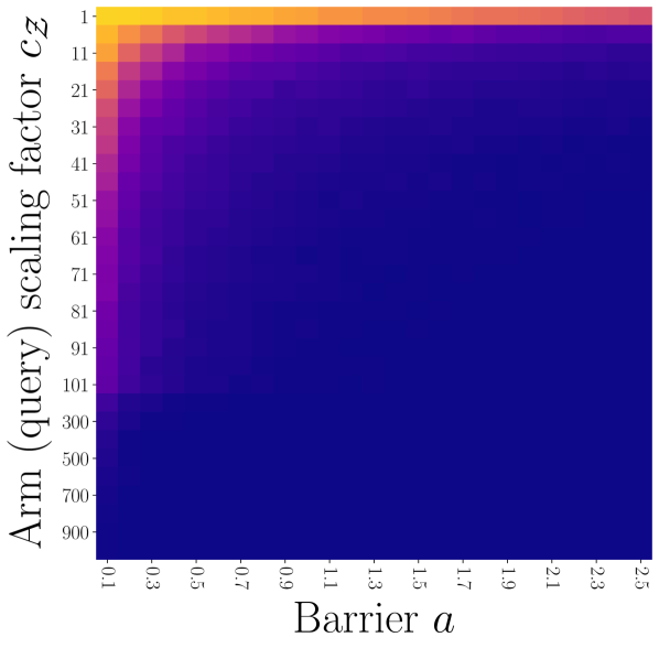
(a) $(\lambda_{\text{trans}},\widehat{\theta}_{\text{CH,DT}})$

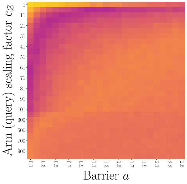
(b) $(\lambda_{\text{trans}},\widehat{\theta}_{\text{CH}})$

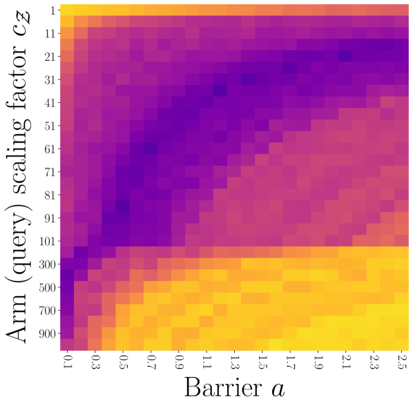
(c) $(\lambda_{\text{hard}},\widehat{\theta}_{\text{CH}})$

Figure 3: Error probability $\mathbb{P}[\operatorname*{arg\,max}_{z\in\mathcal{Z}}z^{\top}\widehat{\theta}\neq z^{*}]$ for three GSE variations, plotted as a function of the arm scaling factor $c_{\mathcal{Z}}$ and the barrier $a$. Darker colors indicate better estimation performance. Each error probability is averaged over $10$ problem instances and $200$ simulations per instance.

As shown in fig. 3(a), our choice-decision-time estimator improves as the barrier $a$ increases, whether $c_{\mathcal{Z}}$ is small (hard queries) or large (easy queries), confirming the theoretical insights from section 3. Additionally, larger $c_{\mathcal{Z}}$ makes best-arm identification easier, enhancing the performance. In fig. 3(b), fixing the barrier $a$ and examining the corresponding vertical line reveals that the choice-only estimator with a transductive design performs well when $c_{\mathcal{Z}}$ is small and queries are hard. However, as $c_{\mathcal{Z}}$ increases and queries become easier, performance declines, despite the task of identifying the best arm becoming easier. This decline, shown by the dark curved band, supports the insights discussed in section 3. Figure 3(c) shows that when $c_{\mathcal{Z}}$ is moderate, the choice-only estimator with a hard-query design outperforms the transductive design (fig. 3(b)), highlighting that focusing on harder queries improves the estimator’s performance. The lower dark band in fig. 3(c) compared to fig. 3(b) indicates that the hard-query design allows the estimator to handle larger $c_{\mathcal{Z}}$ values. However, as $c_{\mathcal{Z}}$ becomes too large, performance declines, likely because many weights $\dot{\mu}(x^{\top}\theta^{*})$ approach zero, excluding informative queries from sampling and negatively impacting performance.

In summary, the empirical results confirm our insights from section 3: easy queries contain less information, but incorporating response times makes them more useful. The hard-query design improves estimation by avoiding easy queries, but this improvement relies on perfect knowledge of $\theta^{*}$ and uniform resource consumption for each query. In realistic scenarios, where $\theta^{*}$ is unknown and hard queries consume longer response times, the hard-query design becomes outperformed by the transductive design, as demonstrated in the next section.

5.2 Fixed-budget best-arm identification performance using real datasets

This section compares the bandit performance of six GSE variations. The first three are as previously defined: $(\lambda_{\text{trans}},\widehat{\theta}_{\text{CH,DT}})$, $(\lambda_{\text{trans}},\widehat{\theta}_{\text{CH}})$, and $(\lambda_{\text{hard}},\widehat{\theta}_{\text{CH}})$. The fourth variation evaluates performance when the non-decision time $t_{\text{nondec}}$ (assumed to be known in section 2) is unknown. By replacing each query’s decision time $t_{x}$ with the response time $t_{\text{RT},x}$ in the choice-decision-time estimator from Eq. (4), we obtain a new GSE variation, denoted by $(\lambda_{\text{trans}},\widehat{\theta}_{\text{CH},\mathbb{RT}})$. The fifth variation is based on Wagenmakers et al. [68, eq. (5)], which states that $x^{\top}\cdot\left(2a\theta^{*}\right)=\mu^{-1}(\mathbb{P}[c_{x}=1])$, where the logit function $\mu^{-1}(p)\coloneqq\log\left(p/\left(1-p\right)\right)$. This leads to the following choice-only estimate of $2a\theta^{*}$:

$$\widehat{\theta}_{\text{CH,logit}}\coloneqq\left(\sum_{x\in\mathcal{X}_{\text{sample}}}n_{x}\>xx^{\top}\right)^{-1}\sum_{x\in\mathcal{X}_{\text{sample}}}n_{x}\>x\cdot\mu^{-1}\left(\widehat{\mathfrak{C}}_{x,i}\right),$$

where $\widehat{\mathfrak{C}}_{x,i}\coloneqq 1/n_{x}\cdot\sum_{i=1}^{n_{x}}\left(c_{x,s_{x,i}}+1\right)/2$ is the empirical mean of the one-zero-coded binary choices. We denote the corresponding GSE variation by $(\lambda_{\text{trans}},\widehat{\theta}_{\text{CH,logit}})$. The sixth variation, denoted by $(\lambda_{\text{trans}},\widehat{\theta}_{\text{CH,DT,logit}})$, is based on Xiang Chiong et al. [74, eq. (6)], which states that $x^{\top}\theta^{*}=\text{sgn}\left(c_{x}\right)\sqrt{\mathbb{E}\left[c_{x}\right]/\mathbb{E}\left[t_{x}\right]\cdot 0.5\>\mu^{-1}\left(\mathbb{P}\left[c_{x}=1\right]\right)}$. This identity forms the basis of the estimator in Berlinghieri et al. [9, eq. (7)]. It also leads to the following choice-decision-time estimate of $\theta^{*}$:

$$\widehat{\theta}_{\text{CH,DT,logit}}\coloneqq\left(\sum_{x\in\mathcal{X}_{\text{sample}}}n_{x}\>xx^{\top}\right)^{-1}\sum_{x\in\mathcal{X}_{\text{sample}}}n_{x}\>x\cdot\text{sgn}\left(c_{x}\right)\sqrt{\frac{\mathbb{E}\left[c_{x}\right]}{\mathbb{E}\left[t_{x}\right]}\cdot 0.5\>\mu^{-1}\left(\widehat{\mathfrak{C}}_{x,i}\right)}.$$

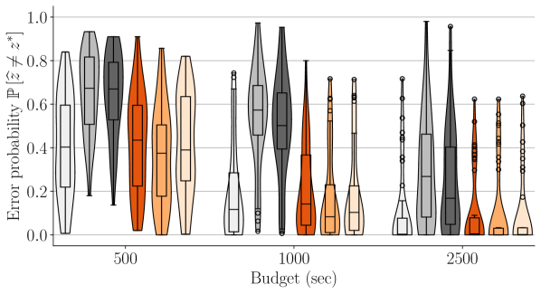
(a) Food-gamble preferences with 0-or-1 choices [58].

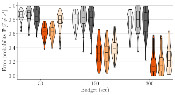
(b) Snack preferences with yes-or-no choices [15].

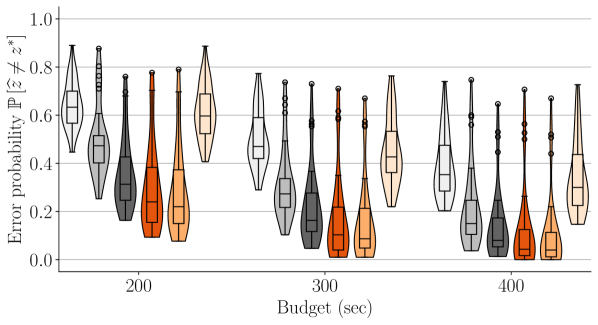
(c) Snack preferences with 0-or-1 choices [38].

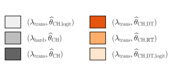
Figure 4: (a), (b), and (c) each presents a violin plot (with an overlaid box plot) for one of the three datasets, showing the distribution of the error probabilities, $\mathbb{P}\left[\widehat{z}\neq z^{*}\right]$, for all bandit instances across various GSE variations and budgets. Each error probability is averaged over $300$ repeated simulations. The box plots follow the conventions used in the matplotlib Python package.

We evaluate the GSE variations by simulating bandit instances constructed from three psychology datasets. The first dataset, on food-gamble preferences [58], contains choices ($0$ or $1$) and response times from $42$ participants answering queries comparing two sets of food items. For each participant, we identified the dEZDM parameters and built a bandit instance with an arm space $\mathcal{Z}\subset\mathbb{R}^{5}$, with $\left|\mathcal{Z}\right|\in[31,95]$, and a query set $\mathcal{X}\coloneqq\left\{z-z^{\prime}\colon z\in\mathcal{Z}\right\}$. The second dataset, on snack preferences [15], contains choices (yes or no) and response times from $31$ participants comparing one snack item to a fixed reference snack. We built a bandit instance for each participant with $\mathcal{Z}\subset\mathbb{R}^{17}$, where $\left|\mathcal{Z}\right|=17$, and $\mathcal{X}\coloneqq\left\{z-\mathbf{0}\colon z\in\mathcal{Z}\right\}$. The third dataset, also on snack preferences [38], contains choices ($0$ or $1$) and response times from $39$ participants comparing two snack items. For each participant, we built a bandit instance with $\mathcal{Z}\subset\mathbb{R}^{21}$, where $\left|\mathcal{Z}\right|=21$, and $\mathcal{X}\coloneqq\left\{z-z^{\prime}\colon z\in\mathcal{Z}\right\}$. For each bandit instance, we tuned the elimination parameter $\eta$ for each GSE variation and simulated them to evaluate performance. Details on data processing and tuning are in appendix D.

The key results for the three domains are shown in fig. 4, with full results in appendix D. First, the GSE variation $(\lambda_{\text{trans}},\widehat{\theta}_{\text{CH,DT}})$ consistently outperformed $(\lambda_{\text{trans}},\widehat{\theta}_{\text{CH}})$, demonstrating the benefit of incorporating response times. This aligns with our theoretical (section 3) and empirical (section 5.1) analyses, showing that response times make better use of easy queries, which also consume less time. Second, both of these GSE variations outperform $(\lambda_{\text{hard}},\widehat{\theta}_{\text{CH}})$. As discussed in section 5.1, this is due to (1) the hard-query design relies on $\widehat{\theta}$ (5 of algorithm 1), which is prone to estimation errors, and (2) the hard-query design favors queries with longer response times, reducing the number of queries sampled under a fixed budget. Third, the GSE variation $(\lambda_{\text{trans}},\widehat{\theta}_{\text{CH,DT}})$ performed similarly to $(\lambda_{\text{trans}},\widehat{\theta}_{\text{CH,}\mathbb{RT}})$, indicating that not knowing the non-decision time has only a minor impact on empirical performance. Finally, the GSE variations $(\lambda_{\text{trans}},\widehat{\theta}_{\text{CH,logit}})$ [68] and $(\lambda_{\text{trans}},\widehat{\theta}_{\text{CH,DT,logit}})$ [74] did not perform as consistently well as $(\lambda_{\text{trans}},\widehat{\theta}_{\text{CH,DT}})$, further highlighting the effectiveness of our proposed choice-decision-time estimator.

6 Limitations and conclusion

Limitations

We have demonstrated the benefits of incorporating response times to accelerate preference learning. However, one key limitation is that high-quality response time data requires participants to remain focused on the task without distraction [45], which can be a challenge in crowdsourcing environments, such as fine-tuning large language models [60, 43, 46, 47, 6]. One potential solution is to integrate human eye movements into the DDM framework, as seen in attentional DDMs [38, 24, 58, 37, 77], to detect lapses in attention. In cases where attention is lost, the system can disregard the response times. From a technical standpoint, a limitation of our work is the lack of full analysis for algorithm 1, which could provide insights into optimizing the elimination parameter $\eta$. Both limitations present promising directions for future research.

Conclusion

In this work, we investigated the incorporation of human response times to enhance fixed-budget best-arm identification in preference-based linear bandits. We proposed an estimator that combines human choices and response times, comparing it against an estimator that uses only choices. Our theoretical and empirical analyses revealed that incorporating response times makes easy queries more useful. We then deployed these estimators in a bandit learning algorithm and demonstrated the superior performance of incorporating response times across simulations based on three datasets.

Appendix A Broader impacts

Incorporating human response times in human-interactive AI systems provides significant benefits, such as efficiently eliciting user preferences, reducing cognitive loads on users, and improving accessibility for users with disabilities and various cognitive abilities. These benefits can greatly improve recommendation systems, assistive robots, online shopping platforms, and fine-tuning for large language models. However, using human response times also raises concerns about privacy, manipulation, and bias against individuals with slower response times. Governments and law enforcement should work together to mitigate these negative consequences by establishing ethical standards and regulations. Businesses should always obtain user consent before recording response times.

Appendix B Literature review

B.1 Bounded accumulation models for choices and response times

Bounded Accumulation Models (BAMs) represent a class of models for human decision-making, typically involving an accumulator (or sampling rule) and a stopping rule [71]. For binary choice tasks, such as two-alternative forced choice tasks, a widely used BAM is the drift-diffusion model (DDM) [51], which consists of a Brownian-motion accumulator and a stopping rule based on two fixed boundaries. To capture the empirical differences in human response times when choosing the correct versus incorrect answer, Ratcliff and McKoon [51] allows the drift, starting point, and non-decision time to randomly vary across trials. Later, Wagenmakers et al. [68] proposed the EZ-diffusion model (EZDM), a simplified version of DDM, offering closed-form expressions for choice and response time moments to simplify the parameter estimation procedure and improve the statistical robustness. EZDM assumes that the drift, starting point, and non-decision time are deterministic and remain fixed across trials and that the starting point is equidistant from the upper and lower boundaries. Recently, Berlinghieri et al. [9] focused on the parameter estimation for the difference-based EZDM, a variant where the drift is the difference in utilities between two options. Formally, for each binary query with arms $z_{1}$ and $z_{2}$, the drift is modeled as the utility difference $u_{z_{1}}-u_{z_{2}}$, where $u_{z_{1}}$ and $u_{z_{2}}$ are the utilities of $z_{1}$ and $z_{2}$.

Our work extends the difference-based EZDDM by parameterizing human utility as a linear function. Specifically, we model each arm’s utility $u_{z}\coloneqq z^{\top}\theta^{*}$, where $\theta^{*}$ represents the human preference vector. This linear parameterization is supported by both the bandit and psychology literature. In the bandit domain, linearly parameterized utility functions can scale effectively in systems with a large number of arms [14, 40]. In psychology, linear combinations of attributes are commonly used to model human multi-attribute decision-making, where individuals focus on different attributes during the decision-making process [65, 24, 77]. One of our empirical studies on food-gamble preferences [58] highlights the potential of our approach for learning human preferences through multi-attribute decision-making.

In a similar vein, recently, Shvartsman et al. [56] parameterize the human utility function as a Gaussian process and propose a moment-matching-based Bayesian inference procedure to estimate the latent utility using both choices and response times. Unlike our work, their focus is solely on estimation, without addressing the bandit optimization aspect. Exploring how their estimation techniques could be integrated into bandit optimization is a promising direction for future research.

Another widely used BAM is the race model [67, 11], which naturally extends to queries with more than two options. In race models, each option has its own accumulator, and the decision-making process ends when any accumulator reaches its threshold. BAMs can also capture human attention during the decision-making process. For example, the attentional-DDM [38, 37, 77] jointly models human choices, response times, and eye movements across various options or attributes in a query. Similarly, Thomas et al. [63] introduce the gaze-weighted linear accumulator model to explore gaze bias effects at the trial level. To incorporate human learning effects, Pedersen et al. [49] integrate reinforcement learning (RL) with DDM to account for the drift’s non-stationarity. In their work, the human uses RL to update their drift, while in our work, the AI agent uses RL to make decisions and interact with the human.

BAMs have theoretical connections to human Bayesian RL models. For example, Fudenberg et al. [25] propose a model where humans face a fixed cost for spending additional time thinking and solve a Bayesian optimal stopping problem to balance this cost with the decision accuracy. Their work shows that this model is equivalent to a DDM with time-decaying boundaries.

Neurophysiological evidence supports BAMs. For instance, EEG recordings demonstrate that neurons exhibit accumulation processes and decision thresholds [71]. Additionally, diffusion processes have been used to model neural firing rates [53].

B.2 Parameter estimation for bounded accumulation models

BAMs typically lack closed-form density functions, making hierarchical Bayesian inference a common approach for parameter estimation [72]. While flexible, these methods are computationally intensive and impractical for real-time use in online learning systems. Fast-computing estimators [68, 9, 74] usually estimate parameters for single option pairs without aggregating data across multiple pairs or leveraging linear parameterization of human utility functions, which is common in large-scale preference learning systems. To address this, our work introduces a computationally efficient estimator for linearly parameterized utility functions, which we integrate into bandit learning. In section 5.2, we empirically show that our estimator outperforms those in prior work [68, 74].

In practice, using response time data requires pre-processing and model fitting, as outlined by Myers et al. [45]. Additionally, Alós-Ferrer et al. [3], Fudenberg et al. [26], Baldassi et al. [7] propose statistical tests to assess the suitability of various DDM extensions for a given dataset.

B.3 Various uses of response times

Response times can serve a variety of objectives, as explored by Clithero [16]. One key use is improving choice prediction. For example, Clithero [15] demonstrated that the EZDM [68] predicts choice probabilities more accurately than the logit model, with parameters estimated via Bayesian Markov chain Monte Carlo. Additionally, Alós-Ferrer et al. [3] showed that response times can enhance the identifiability of human preferences compared to relying on choices alone.

Response times also provide insights into human decision-making processes. Castro et al. [13] used DDM analysis to examine how cognitive workload, induced by secondary tasks, affects decision-making. In fact, analyzing response times has long been used in cognitive testing to assess cognitive capabilities [18]. Furthermore, Zhang et al. [80, 81] proposed a framework that leverages human planning time to infer their targeted goals.

Response times can also enhance AI decision-making. In dueling bandits and preference-based RL [8], human choice models are often used for preference elicitation. One such model, the random utility model, can be derived from certain BAMs [3]. For instance, both the Bradley-Terry model and EZDM yield logistic choice probabilities, which explains why eq. 1, derived from DDM, coincides with the Bradley-Terry model. Both models express the relationship as $\mathbb{P}[z_{1}\succ z_{2}]=1/\left(1+\exp\left(-2a(u_{z_{1}}-u_{z_{2}})\right)\right)$, where $u_{z_{1}}$ and $u_{z_{2}}$ are the utilities of $z_{1}$ and $z_{2}$, respectively. Here, $\sigma_{logistic}$ refers to the logistic link function, as discussed in Bengs et al. [8, section 3.2]. Our work leverages the connection between the random utility model and the choice-response-time model to estimate human utilities using both choices and response times. To the best of our knowledge, our work is the first time this connection has been integrated into the framework of bandit and RL.

We hypothesize that the insight that response times make easy queries useful extends beyond EZDM and the logistic link function. Many psychological models jointly capture choices and response times, but they often lack closed-form distributions for choices. In such cases, choice probability is expressed as $\mathbb{P}[z_{1}\succ z_{2}]=\sigma^{\dagger}(u_{z_{1}},u_{z_{2}})$, where $\sigma^{\dagger}$ could be a complicated function that depends separately on $u_{z_{1}}$ and $u_{z_{2}}$, lacking a closed form. If we fix $u_{z_{2}}$ and vary only $u_{z_{1}}$, the function $\sigma^{\dagger}(\cdot,u_{z_{2}})$ is known as a psychometric function, typically exhibiting an “S” shape, as discussed in Strzalecki [61, the text above fig. 1.1]. Thus, as preference strength becomes either very large or very small, the function value of $\sigma^{\dagger}(\cdot,u_{z_{2}})$ flattens, offering less information—similar to the green curves in figs. 1(b) and 1(c). In these cases, response times can be very useful.

If we assume that choice probability depends only on the utility difference, $u_{z_{1}}-u_{z_{2}}$, then we have $\mathbb{P}[z_{1}\succ z_{2}]=\sigma^{\ddagger}(u_{z_{1}}-u_{z_{2}})$. This $\sigma^{\ddagger}$ serves as the link function commonly used in preference-based RL [8]. According to Bengs et al. [8], $\sigma^{\ddagger}$ is typically assumed to be strictly monotonic in $(u_{z_{1}}-u_{z_{2}})$ and bounded within $[0,1]$, confirming the “S”-shaped behavior. As the utility difference $(u_{z_{1}}-u_{z_{2}})$ becomes either very large or very small, the value $\sigma^{\ddagger}(u_{z_{1}}-u_{z_{2}})$ flattens, offering less information. Thus, we conjecture that response times are crucial in such scenarios.

In summary, bounded accumulation models (BAMs) such as DDMs and race models have a strong theoretical foundation for explaining human decision-making, supported by behavioral and neurophysiological evidence. These models have been applied to both choice prediction and understanding cognitive processes. Our work extends these models to bandits by introducing a computationally efficient estimator for linearly parameterized utility functions. A promising direction for future research is to explore other BAM variants to further examine the benefits of incorporating response times.

Appendix C Proofs

C.1 Parameters of our model - dEZDM

Given a human preference vector $\theta^{*}$ and an EZDM [68] model with a barrier $a$ (introduced in section 2), for each query $x\in\mathcal{X}$, the utility difference $u_{x}\coloneqq x^{\top}\theta^{*}$.

According to Wagenmakers et al. [68, eq. (4), (6), and (9)], the human choice $c_{x}$ has the following properties:

$$\begin{split}\mathbb{P}\left(c_{x}=1\right)=\frac{1}{1+\exp\left(-2au_{x}\right)},\quad\mathbb{P}\left(c_{x}=-1\right)=\frac{\exp\left(-2au_{x}\right)}{1+\exp\left(-2au_{x}\right)}.\end{split}$$

Thus, the expected choice $\mathbb{E}\left[c_{x}\right]=\tanh(au_{x})$ (restating eq. 1) and the variance $\mathbb{V}\left[c_{x}\right]=1-\tanh(a\mu_{x})^{2}$.

The human decision time $t_{x}$ has the following properties:

$$\begin{split}\mathbb{E}\left[t_{x}\right]={}&\begin{cases}\frac{a}{u_{x}}\tanh(au_{x})\quad\text{if }u_{x}\neq 0\\ a^{2}\hfill\text{ if }u_{x}=0\end{cases}\quad\text{(restating \lx@cref{creftype~refnum}{eq:setting:ERT})},\\ \mathbb{V}\left[t_{x}\right]={}&\begin{cases}\frac{a}{u_{x}{}^{3}}\frac{\exp\left(4au_{x}\right)-1-4au_{x}\exp\left(2au_{x}\right)}{\left(\exp\left(2au_{x}\right)+1\right)^{2}}\overset{y\coloneqq-2au_{x}}{=}\frac{a}{u_{x}^{3}}\frac{1-\exp(2y)+2y\exp(y)}{\left(1+\exp(y)\right)^{2}}\quad\text{if }u_{x}\neq 0\\ 2a^{4}/3\hfill\text{ if }u_{x}=0\end{cases}.\end{split}$$

From the above, it is clear that:

$$\begin{split}\frac{\mathbb{E}\left[c_{x}\right]}{\mathbb{E}\left[t_{x}\right]}=\frac{u_{x}}{a}=x^{\top}\left(\frac{1}{a}\theta^{*}\right)\quad\text{(restating \lx@cref{creftype~refnum}{eq:estimation:identity})}.\end{split}$$

Moreover, all the above parameters depend only on the utility difference $u_{x}\coloneqq x^{\top}\theta^{*}$ and the barrier $a$.

C.2 Asymptotic normality of the choice-decision-time estimator for estimating the human preference vector $\theta^{*}$

Here, we provide the proof for theorem 3.1: See 3.1

Proof.

To simplify notation, we define the following:

$$\widehat{\mathcal{C}}_{x}=\frac{1}{n}\sum_{i=1}^{n}c_{x,s_{x,i}},\quad\mathcal{C}_{x}=\mathbb{E}\left[c_{x}\right],\quad\widehat{\mathcal{T}}_{x}=\frac{1}{n}\sum_{i=1}^{n}t_{x,s_{x,i}},\quad\mathcal{T}_{x}=\mathbb{E}\left[t_{x}\right].$$ (8)

For brevity, we abbreviate $\mathcal{X}_{\text{sample}}$ as $\mathcal{X}$ and $\widehat{\theta}_{\text{CH,DT},n}$ as $\widehat{\theta}$. The estimator $\widehat{\theta}$ can be expressed as:

$$\begin{split}\widehat{\theta}=\left(\sum_{x^{\prime}\in\mathcal{X}}nx^{\prime}x^{\prime}{}^{\top}\right)^{-1}\sum_{x\in\mathcal{X}}nx\ \frac{\widehat{\mathcal{C}}_{x}}{\widehat{\mathcal{T}}_{x}}.\end{split}$$ (9)

We rewrite $\theta^{*}/a$ as:

$$\begin{split}\theta^{*}/a={}&\left(\sum_{x^{\prime}\in\mathcal{X}}nx^{\prime}x^{\prime}{}^{\top}\right)^{-1}\sum_{x\in\mathcal{X}}nxx^{\top}\ \frac{\theta^{*}}{a}\\ ={}&\left(\sum_{x^{\prime}\in\mathcal{X}}nx^{\prime}x^{\prime}{}^{\top}\right)^{-1}\sum_{x\in\mathcal{X}}nx\ \frac{\mathcal{C}_{x}}{\mathcal{T}_{x}}.\end{split}$$ (10)

Therefore, for any vector $y\in\mathbb{R}^{d}$, we have:

$$\begin{split}y^{\top}\left(\widehat{\theta}-\frac{\theta^{*}}{a}\right)={}&y^{\top}\left(\sum_{x^{\prime}\in\mathcal{X}}nx^{\prime}x^{\prime}{}^{\top}\right)^{-1}\sum_{x\in\mathcal{X}}nx\left(\frac{\widehat{\mathcal{C}}_{x}}{\widehat{\mathcal{T}}_{x}}-\frac{\mathcal{C}_{x}}{\mathcal{T}_{x}}\right)\eqqcolon\sum_{x\in\mathcal{X}}\xi_{x}\left(\frac{\widehat{\mathcal{C}}_{x}}{\widehat{\mathcal{T}}_{x}}-\frac{\mathcal{C}_{x}}{\mathcal{T}_{x}}\right),\end{split}$$ (11)

where we let $\xi_{x}\coloneqq y^{\top}\left(\sum_{x^{\prime}\in\mathcal{X}}nx^{\prime}x^{\prime}{}^{\top}\right)^{-1}nx$. In eq. 11, the only random variables are $\widehat{\mathcal{C}}_{x}$ and $\widehat{\mathcal{T}}_{x}$. For simplicity, for any $x_{i}\in\mathcal{X}\coloneqq\{x_{1},\cdots,x_{|\mathcal{X}|}\}$, we slighly abuse the notation and let $\xi_{i}$, $c_{i}$, $t_{i}$, $\mathcal{C}_{i}$, $\mathcal{T}_{i}$, $\widehat{\mathcal{C}_{i}}$ and $\widehat{\mathcal{T}_{i}}$ denote $\xi_{x_{i}}$, $c_{x_{i}}$, $t_{x_{i}}$, $\mathcal{C}_{x_{i}}$, $\mathcal{T}_{x_{i}}$, $\widehat{\mathcal{C}}_{x_{i}}$, and $\widehat{\mathcal{T}}_{x_{i}}$, respectively. By the multidimensional central limit theorem, we know:

$$\begin{split}\sqrt{n}\begin{bmatrix}\widehat{\mathcal{C}}_{1}-\mathcal{C}_{1}\\ \widehat{\mathcal{T}}_{1}-\mathcal{C}_{1}\\ \vdots\\ \widehat{\mathcal{C}}_{|\mathcal{X}|}-\mathcal{C}_{|\mathcal{X}|}\\ \widehat{\mathcal{T}}_{|\mathcal{X}|}-\mathcal{C}_{|\mathcal{X}|}\\ \end{bmatrix}\overset{D}{\longrightarrow}{}&\mathcal{N}\left(0,\begin{bmatrix}\mathbb{V}\left[c_{1}\right]&\text{cov}\left[c_{1},t_{1}\right]\\ \text{cov}\left[t_{1},c_{1}\right]&\mathbb{V}\left[t_{1}\right]\\ &&\lx@intercol\hfil\hbox{\multirowsetup$\ddots$}\hfil\lx@intercol\\ \\ &&&&\mathbb{V}\left[c_{|\mathcal{X}|}\right]&\text{cov}\left[c_{|\mathcal{X}|},t_{|\mathcal{X}|}\right]\\ &&&&\text{cov}\left[t_{|\mathcal{X}|},c_{|\mathcal{X}|}\right]&\mathbb{V}\left[t_{|\mathcal{X}|}\right]\\ \end{bmatrix}\right)\\ ={}&\mathcal{N}\Bigg{(}0,\text{diag}\Big{[}\mathbb{V}\left[c_{1}\right],\mathbb{V}\left[t_{1}\right],\cdots,\mathbb{V}\left[c_{|\mathcal{X}|}\right],\mathbb{V}\left[t_{|\mathcal{X}|}\right]\Big{]}\Bigg{)}.\end{split}$$ (12)

Here, in the first line of eq. 12, the block-diagonal structure of the covariance matrix arises because $(\widehat{\mathcal{C}}_{i},\widehat{\mathcal{T}}_{i})_{i\in[|\mathcal{X}|]}$ are independent of each other. To get the second line of eq. 12, for any fixed $x_{i}$, we know:

$$\begin{split}\mathbb{E}\left[t_{i}c_{i}\right]={}&\mathbb{P}\left(c_{i}=1\right)\mathbb{E}\left[1\cdot t_{i}|c_{i}=1\right]+\mathbb{P}\left(c_{i}=-1\right)\mathbb{E}\left[-1\cdot t_{i}|c_{i}=-1\right]\\ \overset{(i)}{=}{}&\left(\mathbb{P}\left(c_{i}=1\right)-\mathbb{P}\left(c_{i}=-1\right)\right)\mathbb{E}\left[t_{i}|c_{i}=1\right]\\ ={}&\mathbb{E}\left[c_{i}\right]\mathbb{E}\left[t_{i}\right],\end{split}$$ (13)

where $(i)$ is because $\mathbb{E}\left[t_{i}|c_{i}=1\right]=\mathbb{E}\left[t_{i}|c_{i}=-1\right]$ [9, eq. (A.7) and (A.9)]. Therefore, eq. 13 implies that $\text{cov}(c_{i},t_{i})=0$ , which justifies the second line of eq. 12.

Now, let function $g(c_{1},t_{1},\cdots,c_{|\mathcal{X}|},t_{|\mathcal{X}|})\coloneqq\sum_{i\in[|\mathcal{X}|]}\xi_{i}\ c_{i}/t_{i}$. The gradient of $g$ is:

$$\begin{split}\nabla g|_{\left(c_{1},t_{1},\cdots,c_{|\mathcal{X}|},t_{|\mathcal{X}|}\right)}=\begin{bmatrix}\xi_{1}/t_{1}&-\xi_{1}c_{1}/t_{1}^{2}&\cdots&\xi_{|\mathcal{X}|}/t_{|\mathcal{X}|}&-\xi_{|\mathcal{X}|}c_{|\mathcal{X}|}/t_{|\mathcal{X}|}^{2}\end{bmatrix}^{\top}.\end{split}$$ (14)

By applying the multivariate delta method, we obtain that:

$$\begin{split}{}&\sqrt{n}\sum_{i\in[|\mathcal{X}|]}\xi_{i}\left(\frac{\widehat{\mathcal{C}}_{i}}{\widehat{\mathcal{T}}_{i}}-\frac{\mathcal{C}_{i}}{\mathcal{T}_{i}}\right)\\ ={}&\sqrt{n}\left(g\left(\widehat{\mathcal{C}}_{1},\widehat{\mathcal{T}}_{1},\cdots,\widehat{\mathcal{C}}_{|\mathcal{X}|},\widehat{\mathcal{T}}_{|\mathcal{X}|}\right)-g\left(\mathcal{C}_{1},\mathcal{T}_{1},\cdots,\mathcal{C}_{|\mathcal{X}|},\mathcal{T}_{|\mathcal{X}|}\right)\right)\\ \overset{D}{\longrightarrow}{}&\mathcal{N}\left(0,\nabla g^{\top}|_{\left(\mathcal{C}_{1},\mathcal{T}_{1},\cdots,\mathcal{C}_{|\mathcal{X}|},\mathcal{T}_{|\mathcal{X}|}\right)}\begin{bmatrix}\mathbb{V}\left[c_{1}\right]\\ &\mathbb{V}\left[t_{1}\right]\\ &&\ddots\\ &&&\mathbb{V}\left[c_{|\mathcal{X}|}\right]&\\ &&&&\mathbb{V}\left[t_{|\mathcal{X}|}\right]\\ \end{bmatrix}\nabla g|_{\left(\mathcal{C}_{1},\mathcal{T}_{1},\cdots,\mathcal{C}_{|\mathcal{X}|},\mathcal{T}_{|\mathcal{X}|}\right)}\right)\\ ={}&\mathcal{N}\left(0,\sum_{i\in[|\mathcal{X}|]}\xi_{i}^{2}\left(\frac{1}{\mathcal{T}_{i}^{2}}\mathbb{V}(c_{i})+\frac{\mathcal{C}_{i}^{2}}{\mathcal{T}_{i}^{4}}\mathbb{V}(t_{i})\right)\right)\\ ={}&\mathcal{N}\left(0,\frac{1}{a^{2}}\sum_{i\in[|\mathcal{X}|]}\xi_{i}^{2}\left(\frac{a^{2}}{\mathcal{T}_{i}^{2}}\mathbb{V}(c_{i})+\frac{a^{2}\mathcal{C}_{i}^{2}}{\mathcal{T}_{i}^{4}}\mathbb{V}(t_{i})\right)\right)\\ \end{split}$$ (15)

Finally, Let $m_{\text{CH,DT}}^{\text{asym}}(x_{i}^{\top}\theta^{*})\coloneqq 1/\left(\frac{a^{2}}{\mathcal{T}_{i}^{2}}\mathbb{V}(c_{i})+\frac{a^{2}\mathcal{C}_{i}^{2}}{\mathcal{T}_{i}^{4}}\mathbb{V}(t_{i})\right)$ and $\mathcal{M}_{\text{CH,DT}}^{\text{asym}}\coloneqq\min_{x}m_{\text{CH,DT}}^{\text{asym}}(x_{i}^{\top}\theta^{*})$, which are abbreviated as $m_{i}$ and $\mathcal{M}$, respectively. The variance can then be upper bounded as follows:

$$\begin{split}{}&\frac{1}{a^{2}}\sum_{i\in[|\mathcal{X}|]}\xi_{i}^{2}\left(\frac{a^{2}}{\mathcal{T}_{i}^{2}}\mathbb{V}(c_{i})+\frac{a^{2}\mathcal{C}_{i}^{2}}{\mathcal{T}_{i}^{4}}\mathbb{V}(t_{i})\right)\leq\frac{1}{a^{2}}\frac{1}{\mathcal{M}}\sum_{i\in[|\mathcal{X}|]}\xi_{i}^{2}\\ \leq{}&\frac{1}{a^{2}}\frac{1}{\mathcal{M}}\cdot\left(\sum_{x\in\mathcal{X}}y^{\top}\left(\sum_{x^{\prime}\in\mathcal{X}}nx^{\prime}x^{\prime}{}^{\top}\right)^{-1}n^{2}xx^{\top}\left(\sum_{x^{\prime}\in\mathcal{X}}nx^{\prime}x^{\prime}{}^{\top}\right)^{-1}y\right)\\ ={}&\frac{1}{a^{2}}\frac{1}{\mathcal{M}}\cdot y^{\top}\left(\sum_{x^{\prime}\in\mathcal{X}}x^{\prime}x^{\prime}{}^{\top}\right)^{-1}y\\ ={}&\frac{1}{a^{2}}y^{\top}\left(\sum_{x^{\prime}\in\mathcal{X}}\mathcal{M}x^{\prime}x^{\prime}{}^{\top}\right)^{-1}y\\ \equiv{}&\frac{1}{a^{2}}\left\|y\right\|_{\left(\sum_{x^{\prime}\in\mathcal{X}}\mathcal{M}x^{\prime}x^{\prime}{}^{\top}\right)^{-1}}^{2}.\end{split}$$ (16)

∎

C.3 Non-asymptotic concentration of the two estimators for estimating the utility difference $u_{x}$ given a query $x$

C.3.1 The choice-decision-time estimator

Section 3.3 addresses the problem of estimating the utility difference for a single query. Specifically, for a given query $x\in\mathcal{X}$, the goal is to estimate the utility difference $u_{x}\coloneqq x^{\top}\theta^{*}$ based on the i.i.d. dataset $\left\{(c_{x,s_{x,i}},t_{x,s_{x,i}})\right\}_{i\in[n_{x}]}$.

We begin by applying the linear-regression-based choice-decision-time estimator from eq. 4, to this problem. This estimator is derived as the solution to the following least squares problem:

$$\begin{split}\widehat{\theta}_{\text{CH,DT}}=\operatorname*{arg\,min}_{\theta\in\mathbb{R}^{d}}\sum_{x\in\mathcal{X}_{\text{sample}}}\left(x^{\top}\theta-\frac{\sum_{i\in[n_{x}]}c_{x,s_{x,i}}}{\sum_{i\in[n_{x}]}t_{x,s_{x,i}}}\right)^{2}.\end{split}$$

Similarly, the utility difference estimator for a single query can be derived as the solution to the following least squares problem, yielding the following estimate:

$$\begin{split}\widehat{u}_{x,\text{CH,DT}}=\operatorname*{arg\,min}_{u\in\mathbb{R}}\left(u-\frac{\sum_{i\in[n_{x}]}c_{x,s_{x,i}}}{\sum_{i\in[n_{x}]}t_{x,s_{x,i}}}\right)^{2}=\frac{\sum_{i\in[n_{x}]}c_{x,s_{x,i}}}{\sum_{i\in[n_{x}]}t_{x,s_{x,i}}}\quad\text{(restating \lx@cref{creftype~refnum}{eq:estimation:GLM:singleQuery})}.\end{split}$$

The estimate, $\widehat{u}_{x,\text{CH,DT}}$, is an estimate for $u_{x}/a$, not $u_{x}$. However, since the ranking of arm utilities based on $u_{x}/a$ is the same as the one based on the true $u_{x}$, estimating $u_{x}/a$ is sufficient for best-arm identification.

Assuming the utility difference, $u_{x}\neq 0$, this estimator’s non-asymptotic concentration inequality is presented in theorem 3.3. To prove this, we first present lemma C.1, which shows that for each query $x$, the empirical mean decision time is a sub-exponential random variable.

For simplicity, we introduce the following notations:

$$\widehat{\mathcal{C}}_{x}=\frac{1}{n_{x}}\sum_{i=1}^{n_{x}}c_{x,s_{x,i}},\quad\mathcal{C}_{x}=\mathbb{E}\left[c_{x}\right],\quad\widehat{\mathcal{T}}_{x}=\frac{1}{n_{x}}\sum_{i=1}^{n_{x}}t_{x,s_{x,i}},\quad\mathcal{T}_{x}=\mathbb{E}\left[t_{x}\right],\quad\widehat{u}_{x,\text{CH,DT}}=\frac{\widehat{\mathcal{C}}_{x}}{\widehat{\mathcal{T}}_{x}}.$$ (17)

Lemma C.1.

If $u_{x}\neq 0$, then $\widehat{\mathcal{T}}_{x}-\mathcal{T}_{x}$ is sub-exponential $\text{SE}\left(\nu_{x}^{2},\alpha_{x}\right)$, where $\nu_{x}=\sqrt{2}a/|u_{x}|$ and $\alpha_{x}=2/u_{x}^{2}$.

Proof.

For simplicity, we will drop the subscript $x$ throughout this proof and assume without loss of generality that $u>0$.

Our goal is to prove the following inequality, which holds for all $s\in(-u^{2}/2,u^{2}/2)$:

$$\begin{split}\mathbb{E}\left(\exp\left(s\left(\widehat{\mathcal{T}}-\mathcal{T}\right)\right)\right)\leq\exp\left(\frac{2a^{2}/u^{2}}{2}s^{2}\right).\end{split}$$ (18)

which implies that $\widehat{\mathcal{T}}_{x}-\mathcal{T}_{x}$ is sub-exponential $\text{SE}\left(\nu_{x}^{2},\alpha_{x}\right)$ according to Wainwright [70, Definition 2.7].

Step 1. Transform eq. 18 into another inequality (eq. 24) that is easier to prove.

From Cox [17, eq. (128)], with $\Delta\coloneqq u^{2}-2s$, $\theta_{1}\coloneqq-u-\sqrt{\Delta}$ and $\theta_{2}\coloneqq-u+\sqrt{\Delta}$, we have

$$\begin{split}\mathbb{E}\left(\exp\left(s\widehat{\mathcal{T}}\right)\right)={}&\frac{\exp\left(a\theta_{1}\right)-\exp\left(2a\theta_{2}+a\theta_{1}\right)}{\exp\left(2a\theta_{1}\right)-\exp\left(2a\theta_{2}\right)}-\frac{\exp\left(a\theta_{2}\right)-\exp\left(2a\theta_{1}+a\theta_{2}\right)}{\exp\left(2a\theta_{1}\right)-\exp\left(2a\theta_{2}\right)}\\ ={}&\frac{\exp\left(a\theta_{1}\right)\left[1+\exp\left(a\theta_{1}+a\theta_{2}\right)\right]}{\exp\left(2a\theta_{1}\right)-\exp\left(2a\theta_{2}\right)}-\frac{\exp\left(a\theta_{2}\right)\left[1+\exp\left(a\theta_{2}+a\theta_{1}\right)\right]}{\exp\left(2a\theta_{1}\right)-\exp\left(2a\theta_{2}\right)}\\ ={}&\frac{\left[\exp\left(a\theta_{1}\right)-\exp\left(a\theta_{2}\right)\right]\left[1+\exp\left(a\theta_{2}+a\theta_{1}\right)\right]}{\exp\left(2a\theta_{1}\right)-\exp\left(2a\theta_{2}\right)}\\ ={}&\frac{1+\exp\left(a\theta_{2}+a\theta_{1}\right)}{\exp\left(a\theta_{1}\right)+\exp\left(a\theta_{2}\right)}\\ ={}&\frac{\exp\left(-au\right)+\exp\left(au\right)}{\exp\left(-a\sqrt{\Delta}\right)+\exp\left(a\sqrt{\Delta}\right)}\\ \eqqcolon{}&\frac{N}{D(s)}.\end{split}$$ (19)

In the last line, we define $N=2\cosh(au)$ and $D(s)=2\cosh(a\sqrt{\Delta})$. Thus, we arrive at:

$$\begin{split}\mathbb{E}\left(\exp\left(s\cdot\left(\widehat{\mathcal{T}}-\mathcal{T}\right)\right)\right)=\frac{N}{D(s)}\cdot\frac{1}{\exp\left(s\cdot\mathcal{T}\right)}=\frac{N}{\exp\left(sa\tanh(au)/u\right)D(s)}.\end{split}$$ (20)

Now, to prove the original inequality in eq. 18, it is sufficient to show:

$$\begin{split}D(s)\cdot\exp\left(\frac{a}{u}\tanh(au)s+\frac{a^{2}}{u^{2}}s^{2}\right)\geq N.\end{split}$$ (21)

When $s=0$, this inequality holds trivially because:

$$\begin{split}D(0)\cdot 1=2\cosh(au)=N.\end{split}$$ (22)

For $s\neq 0$, by taking the derivative of the left-hand-side of eq. 21, we obtain the following:

$$\begin{split}{}&\frac{\text{d}}{\text{d}s}\left(D(s)\cdot\exp\left(\frac{a}{u}\tanh(au)s+\frac{a^{2}}{u^{2}}s^{2}\right)\right)\\ ={}&\exp\left(\frac{a}{u}\tanh(au)s+\frac{a^{2}}{u^{2}}s^{2}\right)\cdot\left(-\frac{2a}{\sqrt{\Delta}}\sinh\left(a\sqrt{\Delta}\right)+2\cosh\left(a\sqrt{\Delta}\right)\cdot\left(\frac{a}{u}\tanh(au)+2\frac{a^{2}}{u^{2}}s\right)\right)\\ ={}&2\exp\left(\frac{a}{u}\tanh(au)s+\frac{a^{2}}{u^{2}}s^{2}\right)\cosh\left(a\sqrt{\Delta}\right)\cdot\left(-\frac{a}{\sqrt{\Delta}}\tanh\left(a\sqrt{\Delta}\right)+\frac{a}{u}\tanh(au)+2\frac{a^{2}}{u^{2}}s\right).\end{split}$$ (23)

In step 2, we will prove the following inequality:

$$\begin{split}-\frac{a}{\sqrt{\Delta}}\tanh\left(a\sqrt{\Delta}\right)+\frac{a}{u}\tanh(au)+2\frac{a^{2}}{u^{2}}s\left\{\begin{array}[]{ll}\geq 0,&\forall s\geq 0,\\ <0,&\forall s<0,\\ \end{array}\right.\end{split}$$ (24)

Equation 24 implies that $D(s)\cdot\exp\left(\frac{a}{u}\tanh(au)s+\frac{a^{2}}{u^{2}}s^{2}\right)\geq N$, which finishes the proof.

Step 2. Prove eq. 24.

For $s\geq 0$, the following holds:

$$\begin{split}{}&-\frac{a}{\sqrt{\Delta}}\tanh\left(a\sqrt{\Delta}\right)+\frac{a}{u}\tanh(au)+2\frac{a^{2}}{u^{2}}s\\ \overset{(i)}{\geq}{}&a\tanh\left(a\sqrt{\Delta}\right)\left(\frac{1}{u}-\frac{1}{\sqrt{\Delta}}\right)+2\frac{a^{2}}{u^{2}}s\\ ={}&a\tanh\left(a\sqrt{\Delta}\right)\frac{-2s}{u\sqrt{\Delta}\left(\sqrt{\Delta}+u\right)}+2\frac{a^{2}}{u^{2}}s\\ ={}&-2s\cdot\frac{a^{2}}{u\left(\sqrt{\Delta}+u\right)}\cdot\frac{\tanh\left(a\sqrt{\Delta}\right)}{a\sqrt{\Delta}}+2\frac{a^{2}}{u^{2}}s\\ \overset{(ii)}{\geq}{}&-2s\frac{a^{2}}{u^{2}}\cdot 1+2\frac{a^{2}}{u^{2}}s\\ ={}&0.\end{split}$$ (25)

Here, $(i)$ follows from $\tanh(au)\geq\tanh(a\sqrt{\Delta})=\tanh(a\sqrt{u^{2}-2s})$ and $(ii)$ follows from $\tanh(x)/x\leq 1$.

For $s<0$, the following holds:

$$\begin{split}{}&-\frac{a}{\sqrt{\Delta}}\tanh\left(a\sqrt{\Delta}\right)+\frac{a}{u}\tanh(au)+2\frac{a^{2}}{u^{2}}s\\ \overset{(i)}{\leq}{}&a\tanh\left(a\sqrt{\Delta}\right)\left(\frac{1}{u}-\frac{1}{\sqrt{\Delta}}\right)+2\frac{a^{2}}{u^{2}}s\\ ={}&-2s\cdot\frac{a^{2}}{u\left(\sqrt{\Delta}+u\right)}\cdot\frac{\tanh\left(a\sqrt{\Delta}\right)}{a\sqrt{\Delta}}+2\frac{a^{2}}{u^{2}}s\\ \overset{(ii)}{\leq}{}&-2s\frac{a^{2}}{u^{2}}\cdot 1+2\frac{a^{2}}{u^{2}}s\\ ={}&0.\end{split}$$ (26)

Here, $(i)$ follows from $\tanh(au)\leq\tanh(a\sqrt{\Delta})=\tanh(a\sqrt{u^{2}-2s})$ and $(ii)$ follows from $\tanh(x)/x\leq 1$.

By combining both cases, we conclude that the inequality in eq. 24 holds, which completes Step 2 and proves the desired result. ∎

Next, we prove theorem 3.3, which presents the non-asymptotic concentration inequality for the estimator from eq. 7. See 3.3

Proof.

For clarity, we will omit the subscripts $x$ throughout this proof. Based on lemma C.1, we define the constants $\nu\coloneqq\sqrt{2}a/|u|$ and $\alpha\coloneqq 2/u^{2}$.

We begin by introducing $\epsilon_{\mathcal{C}}\coloneqq\mathcal{T}/\left(\sqrt{2}+\sqrt{2}\nu|\mathcal{C}|/\mathcal{T}\right)\cdot\epsilon$ and $\epsilon_{\mathcal{T}}\coloneqq\nu\epsilon_{\mathcal{C}}$. By $\nu|\mathcal{C}|/\mathcal{T}=\sqrt{2}a/|u|\cdot|u|/a=\sqrt{2}$, we simplify the two constants to:

$$\begin{split}\epsilon_{\mathcal{C}}=\frac{\mathcal{T}}{\sqrt{2}\left(\sqrt{2}+1\right)}\epsilon\quad\text{and}\quad\epsilon_{\mathcal{T}}=\frac{\nu\mathcal{T}}{\sqrt{2}\left(\sqrt{2}+1\right)}\epsilon.\end{split}$$ (27)

For any $\epsilon$ that satisfies the following condition:

$$\begin{split}\epsilon\leq\min\left\{\frac{1}{\nu},\frac{\sqrt{2}(1+\sqrt{2})\nu}{\alpha\mathcal{T}}\right\},\end{split}$$ (28)

we know that $\epsilon_{\mathcal{T}}<\min\left\{\mathcal{T}(1-1/\sqrt{2}),\nu^{2}/\alpha\right\}$. So we apply lemma C.2 and obtain the following:

$$\begin{split}\mathbb{P}\left(\left|\widehat{\mathcal{T}}-\mathcal{T}\right|>\epsilon_{\mathcal{T}}\right)\leq{}&2\exp\left(-\frac{n\epsilon_{\mathcal{T}}^{2}}{2\nu^{2}}\right).\end{split}$$ (29)

Therefore, by combining the results so far, we conclude:

$$\begin{split}\mathbb{P}\left(\left|\frac{\widehat{\mathcal{C}}}{\widehat{\mathcal{T}}}-\frac{\mathcal{C}}{\mathcal{T}}\right|>\epsilon\right)={}&\mathbb{P}\left(\left|\frac{\widehat{\mathcal{C}}}{\widehat{\mathcal{T}}}-\frac{\mathcal{C}}{\mathcal{T}}\right|>\sqrt{2}\frac{\epsilon_{\mathcal{C}}+\epsilon_{\mathcal{T}}\cdot|\mathcal{C}|/\mathcal{T}}{\mathcal{T}}\right)\\ \overset{(i)}{\leq}{}&\mathbb{P}\left(\left|\widehat{\mathcal{C}}-\mathcal{C}\right|>\epsilon_{\mathcal{C}}\right)+\mathbb{P}\left(\left|\widehat{\mathcal{T}}-\mathcal{T}\right|>\epsilon_{\mathcal{T}}\right)\\ \overset{(ii)}{\leq}{}&2\exp\left(-\frac{n\epsilon_{\mathcal{C}}^{2}}{2}\right)+2\exp\left(-\frac{n\epsilon_{\mathcal{T}}^{2}}{2\nu^{2}}\right)\\ \overset{(iii)}{=}{}&4\exp\left(-\frac{n\epsilon_{\mathcal{C}}^{2}}{2}\right)\\ ={}&4\exp\left(-\frac{\mathcal{T}^{2}}{4\left(1+\sqrt{2}\right)^{2}}\cdot n\epsilon^{2}\right).\end{split}$$ (30)

Here, $(i)$ follows from lemma C.3, $(ii)$ uses lemma C.2 and eq. 29, and $(iii)$ follows from eq. 27. ∎

Supporting Details

Lemma C.2.

For each query $x$ with $u_{x}\neq 0$, and constants $\epsilon_{\mathcal{C}}>0$ and $\epsilon_{\mathcal{T}}\in(0,\nu_{x}^{2}/\alpha_{x}]$, the following holds:

$$\begin{split}\mathbb{P}\left(\left|\widehat{\mathcal{C}}_{x}-\mathcal{C}_{x}\right|\geq\epsilon_{\mathcal{C}}\right)\leq 2\exp\left(-\frac{n\epsilon_{\mathcal{C}}^{2}}{2}\right),\quad\mathbb{P}\left(\left|\widehat{\mathcal{T}}_{x}-\mathcal{T}_{x}\right|\geq\epsilon_{\mathcal{T}}\right)\leq 2\exp\left(-\frac{n\epsilon_{\mathcal{T}}^{2}}{2\nu_{x}^{2}}\right).\end{split}$$ (31)

Here, the constants $\nu_{x}\coloneqq\sqrt{2}a/|u_{x}|$ and $\alpha_{x}\coloneqq 2/u_{x}^{2}$.

Proof.

Since $c_{x}\in\{-1,1\}$, by Hoeffding’s inequality [70, proposition 2.5], we obtain:

$$\begin{split}\mathbb{P}\left(\left|\widehat{\mathcal{C}}_{x}-\mathcal{C}_{x}\right|\geq\epsilon_{\mathcal{C}}\right)\leq 2\exp\left(-\frac{n\epsilon_{\mathcal{C}}^{2}}{2}\right).\end{split}$$ (32)

From lemma C.1, we know that $\mathcal{T}_{x}$ is sub-exponential $SE(\nu_{x}^{2},\alpha_{x})$. By applying Wainwright [70, proposition 2.9 and eq. (2.18)], we obtain:

$$\begin{split}\mathbb{P}\left(\left|\widehat{\mathcal{T}}_{x}-\mathcal{T}_{x}\right|\geq\epsilon_{\mathcal{T}}\right)\leq 2\exp\left(-\frac{n\epsilon_{\mathcal{T}}^{2}}{2\nu_{x}^{2}}\right),\quad\forall\epsilon_{\mathcal{T}}\in(0,\nu_{x}^{2}/\alpha_{x}].\end{split}$$ (33)

∎

Lemma C.3.

Consider any constants $\mathcal{C}\in\mathbb{R}$, $\mathcal{T}>0$, $\epsilon_{\mathcal{C}}>0$, and $\epsilon_{\mathcal{T}}\in\left(0,(1-1/\sqrt{2})\mathcal{T}\right)$. Then, for any $\widehat{\mathcal{C}}\in[\mathcal{C}-\epsilon_{\mathcal{C}},\mathcal{C}+\epsilon_{\mathcal{C}}]$ and $\widehat{\mathcal{T}}\in[\mathcal{T}-\epsilon_{\mathcal{T}},\mathcal{T}+\epsilon_{\mathcal{T}}]$, the following holds

$$\begin{split}\left|\frac{\widehat{\mathcal{C}}}{\widehat{\mathcal{T}}}-\frac{\mathcal{C}}{\mathcal{T}}\right|\leq\sqrt{2}\frac{\epsilon_{\mathcal{C}}+\epsilon_{\mathcal{T}}\cdot|\mathcal{C}|/\mathcal{T}}{\mathcal{T}}.\end{split}$$ (34)

Proof.

The maximum of $\left|\widehat{\mathcal{C}}/\widehat{\mathcal{T}}-\mathcal{C}/\mathcal{T}\right|$ is attained at the extremum of $\widehat{\mathcal{C}}/\widehat{\mathcal{T}}$. Since $\widehat{\mathcal{C}}/\widehat{\mathcal{T}}$ is linear in $\widehat{\mathcal{C}}$, the extremum of $\widehat{\mathcal{C}}/\widehat{\mathcal{T}}$ is attained at $C^{*}\in\{\mathcal{C}-\epsilon_{\mathcal{C}},\mathcal{C}+\epsilon_{\mathcal{C}}\}$ for any $\widehat{\mathcal{T}}\in[\mathcal{T}-\epsilon_{\mathcal{T}},\mathcal{T}+\epsilon_{\mathcal{T}}]>0$. Moreover, since $\widehat{\mathcal{T}}>0$, the extremum of $C^{*}/\widehat{\mathcal{T}}$ is attained at $T^{*}\in\{\mathcal{T}-\epsilon_{\mathcal{T}},\mathcal{T}+\epsilon_{\mathcal{T}}\}$. Therefore, the extremum of $\widehat{\mathcal{C}}/\widehat{\mathcal{T}}$ lies in the following set:

$$\begin{split}\max_{\begin{subarray}{c}\widehat{\mathcal{C}}\in[\mathcal{C}-\epsilon_{\mathcal{C}},\mathcal{C}+\epsilon_{\mathcal{C}}]\\ \widehat{\mathcal{T}}\in[\mathcal{T}-\epsilon_{\mathcal{T}},\mathcal{T}+\epsilon_{\mathcal{T}}]\end{subarray}}\frac{\widehat{\mathcal{C}}}{\widehat{\mathcal{T}}}\in\left\{\frac{\mathcal{C}-\epsilon_{\mathcal{C}}}{\mathcal{T}-\epsilon_{\mathcal{T}}},\quad\frac{\mathcal{C}-\epsilon_{\mathcal{C}}}{\mathcal{T}+\epsilon_{\mathcal{T}}},\quad\frac{\mathcal{C}+\epsilon_{\mathcal{C}}}{\mathcal{T}-\epsilon_{\mathcal{T}}},\quad\frac{\mathcal{C}+\epsilon_{\mathcal{C}}}{\mathcal{T}+\epsilon_{\mathcal{T}}}\right\}.\end{split}$$ (35)

Moreover, for any pair $(s_{\mathcal{C}},s_{\mathcal{T}})\in\{\pm 1\}\times\{\pm 1\}$, since $\epsilon_{\mathcal{T}}\leq(1-1/\sqrt{2})\mathcal{T}$, we have:

$$\begin{split}{}&\left|\frac{\mathcal{C}+s_{\mathcal{C}}\epsilon_{\mathcal{C}}}{\mathcal{T}+s_{\mathcal{T}}\epsilon_{\mathcal{T}}}-\frac{\mathcal{C}}{\mathcal{T}}\right|=\left|\frac{s_{\mathcal{C}}\epsilon_{\mathcal{C}}\mathcal{T}-s_{\mathcal{T}}\epsilon_{\mathcal{T}}\mathcal{C}}{\mathcal{T}\left(\mathcal{T}+s_{\mathcal{T}}\epsilon_{\mathcal{T}}\right)}\right|\leq\frac{\epsilon_{\mathcal{C}}\mathcal{T}+\epsilon_{\mathcal{T}}|\mathcal{C}|}{\mathcal{T}\left(\mathcal{T}-\epsilon_{\mathcal{T}}\right)}\leq\sqrt{2}\frac{\epsilon_{\mathcal{C}}\mathcal{T}+\epsilon_{\mathcal{T}}|\mathcal{C}|}{\mathcal{T}^{2}}.\end{split}$$ (36)

Combining the above results, we conclude:

$$\begin{split}\max_{\begin{subarray}{c}\widehat{\mathcal{C}}\in[\mathcal{C}-\epsilon_{\mathcal{C}},\mathcal{C}+\epsilon_{\mathcal{C}}]\\ \widehat{\mathcal{T}}\in[\mathcal{T}-\epsilon_{\mathcal{T}},\mathcal{T}+\epsilon_{\mathcal{T}}]\end{subarray}}\left|\frac{\widehat{\mathcal{C}}}{\widehat{\mathcal{T}}}-\frac{\mathcal{C}}{\mathcal{T}}\right|={}&\max_{(s_{\mathcal{C}},s_{\mathcal{T}})\in\{\pm 1\}\times\{\pm 1\}}\left|\frac{\mathcal{C}+s_{\mathcal{C}}\epsilon_{\mathcal{C}}}{\mathcal{T}+s_{\mathcal{T}}\epsilon_{\mathcal{T}}}-\frac{\mathcal{C}}{\mathcal{T}}\right|\leq\sqrt{2}\frac{\epsilon_{\mathcal{C}}+\epsilon_{\mathcal{T}}|\mathcal{C}|/\mathcal{T}}{\mathcal{T}}.\end{split}$$

∎

C.3.2 The choice-only estimator

We apply the logistic-regression-based choice-only estimator from eq. 5 to the problem. Recall that for each query $x\in\mathcal{X}$, the human choice $c_{x}\in\{-1,1\}$. Now, let’s define the binary-encoded choice as $e_{x}\coloneqq\left(c_{x}+1\right)/2\in\{0,1\}$. We then reduce the MLE formulated in eq. 5 to the problem of utility difference estimation for a single query and obtain the following optimization program:

$$\begin{split}\widehat{u}_{x,\text{CH}}={}&\operatorname*{arg\,max}_{u\in\mathbb{R}}\sum_{i\in[n_{x}]}\log\mu(c_{x,s_{x,i}}\>u)\\ ={}&\operatorname*{arg\,max}_{u\in\mathbb{R}}\sum_{i\in[n_{x}]}\log\left[\left(\mu(u)\right)^{e_{x,s_{x,i}}}\cdot\left(\mu(-u)\right)^{1-e_{x,s_{x,i}}}\right].\end{split}$$

The first-order optimality condition leads to the following optimal solution:

$$\widehat{u}_{x,\text{CH}}=\mu^{-1}\left(\frac{1}{n_{x}}\sum_{i\in[n_{x}]}e_{x,s_{x,i}}\right)\quad\text{(restating \lx@cref{creftype~refnum}{eq:estimation:GLM:singleQuery})},$$

where $\mu^{-1}(p)\coloneqq\log\left(p/(1-p)\right)$ is the logit function (also known as the log-odds), defined as the inverse of the function $\mu(\cdot)$ introduced in eq. 5.

The estimate, $\widehat{u}_{x,\text{CH}}$, in eq. 7 is an estimate for $2au_{x}$, not $u_{x}$. However, since the ranking of arm utilities based on $2au_{x}$ is the same as the one based on the true $u_{x}$, estimating $2au_{x}$ is sufficient for best-arm identification.

This estimator’s non-asymptotic concentration is stated in theorem 3.4. This result can be directly adapted from Jun et al. [30, theorem 1] by setting the arm and query spaces to contain only a single element with the $1$-dimensional feature vector $[1]$.

Appendix D Experiment details

Our implementation of algorithm 1 is done in Julia, building on the work of Tirinzoni and Degenne [64], where the transductive and hard-query designs are solved using the Frank–Wolfe algorithm [22]. Their implementation is available at https://github.com/AndreaTirinzoni/bandit-elimination. The simulation and Bayesian inference for DDM are implemented using the Julia package SequentialSamplingModels.jl at https://itsdfish.github.io/SequentialSamplingModels.jl/dev/#SequentialSamplingModels.jl.

For a query $x\in\mathcal{X}$, the estimators based on Wagenmakers et al. [68] and Xiang Chiong et al. [74], which were theoretically analyzed in section 3.3 and empirically benchmarked in section 5.2, require the computation $\mu^{-1}(p)\coloneqq\log\left(p/\left(1-p\right)\right)$, where $\mu^{-1}(\cdot)$ is the logit function and $p\coloneqq 1/n_{x}\cdot\sum_{i=1}^{n_{x}}\left(c_{x,s_{x,i}}+1\right)/2$ represents the empirical mean of the one-zero-coded binary human choices. In practice, $p$ can sometimes be $0$ or $1$, making this calculation undefined. To address this, we follow the procedure from Wagenmakers et al. [68, the discussion below fig. 6], approximating $p$ as $1-1/(2n_{x})$ when $p=1$ and as $1/(2n_{x})$ when $p=0$.

D.1 Processing the dataset of food-gamble preferences with 0-or-1 choices [58]

We accessed this dataset through Yang and Krajbich [77]’s data at https://osf.io/d7s6c/. The dataset [58] includes the choices and response times of $42$ participants, each responding to between $60$ and $200$ queries. Each query compares two arms, with each arm containing two food items. By selecting an arm, participants had an equal chance of receiving either food item, hence the name “food gamble” task. Additionally, participants’ eye movements were tracked during the experiment. Yang and Krajbich [77] modeled each participant’s choices, response times, and eye movements using the attentional DDM [38], where the drift for each query is a linear combination of the participant’s ratings of the four food items in the query, with the weights adjusting based on their eye movements. The ratings, $\in\{-10,-9,\dots,0,\dots,9,10\}$, were collected before the participants interacted with the binary queries.

In our work, for each participant, we define each arm’s feature vector as the participant’s ratings of the two corresponding food items, augmented with second-order polynomials. Since our focus is not on human attention or eye movements, we fit each participant’s data to our difference-based EZ-diffusion model [68, 9], where the drifts are linear in the feature space with a fixed weight vector $\theta^{*}\in\mathbb{R}^{5}$, as outlined in section 2. Using Bayesian inference with non-informative priors [16], we estimated the preference vector $\theta^{*}$, non-decision time $t_{\text{nondec}}$, and barrier $a$. Across participants, the barrier $a$ ranged from $0.715$ to $2.467$, with a mean of $1.437$, and $t_{\text{nondec}}$ ranged from $0.206$ to $1.917$ seconds, with a mean of $0.746$ seconds. This procedure generates one bandit instance per participant, with a preference vector $\theta^{*}\in\mathbb{R}^{5}$, an arm set $\mathcal{Z}\subset\mathbb{R}^{5}$ where $\left|\mathcal{Z}\right|\in[31,95]$, and a query set $\mathcal{X}\coloneqq\left\{z-z^{\prime}\colon z\in\mathcal{Z}\right\}$.

For each bandit instance, we benchmarked six GSE variations (introduced in section 5.2): $(\lambda_{\text{trans}},\widehat{\theta}_{\text{CH,DT}})$, $(\lambda_{\text{trans}},\widehat{\theta}_{\text{CH,}\mathbb{RT}})$, $(\lambda_{\text{trans}},\widehat{\theta}_{\text{CH}})$, $(\lambda_{\text{hard}},\widehat{\theta}_{\text{CH}})$, $(\lambda_{\text{trans}},\widehat{\theta}_{\text{CH,logit}})$, and $(\lambda_{\text{trans}},\widehat{\theta}_{\text{CH,DT,logit}})$. For each GSE variation, we ran $300$ repeated simulations under different random seeds, with human choices and response times sampled from the dEZDM with the identified parameters. Since each bandit instance contains a different number of arms, rather than tuning the elimination parameter $\eta$ in algorithm 1 for each instance, we set $\eta=2$, following the convention in previous bandit research, e.g., Azizi et al. [4, section 3]. The full results are shown in fig. 5, with selected results highlighted in fig. 4(a).

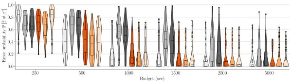
Figure 5: A violin plot overlaid with a box plot showing the best-arm identification error probability, $\mathbb{P}\left[\widehat{z}\neq z^{*}\right]$, as a function of budget for each GSE variation, simulated using the dataset of food-gamble preferences [58], as described in section D.1. The box plots follow the convention of the matplotlib Python package. For each GSE variation and budget, the horizontal line in the middle of the box represents the median of the error probabilities across all bandit instances. Each error probability is averaged over $300$ repeated simulations under different random seeds. The box’s upper and lower borders represent the third and first quartiles, respectively, with whiskers extending to the farthest points within $1.5\times$ the interquartile range. Flier points indicate outliers beyond the whiskers.

D.2 Processing the dataset of snack preferences with yes-or-no choices [15]

We accessed this dataset through Alós-Ferrer et al. [3]’s supplementary material at https://www.journals.uchicago.edu/doi/abs/10.1086/713732. The dataset [15] has a training and a testing datasets. The training dataset was collected from a “YN” task. In each trial, each of the $31$ participants provides binary feedback (“Yes” or “No”), alongside response times to queries between each one of the $17$ snack items and a reference snack item, where each query was repeated for $10$ times. The reference item, with $0$ utility, was predetermined and remained fixed throughout the entire experiment. On the other hand, the testing task was collected from a two-alternative forced-choice task where each participant provides binary choice feedback, alongside response times, to queries between two of the $17$ snack items, where each query was repeated for $1$ times. This paper fits an EZDM [68] using Bayesian inference with non-informative priors to each participant’s training dataset from the “YN” task and tests the identified model using the testing dataset from the two-alternative forced-choice task. Accordingly, in our work, we use the training dataset to identify DDM models, which are then used to simulate the bandit human feedback.

Clithero [15] includes both a training and a testing dataset. The training dataset was collected from a “Yes/No” task, in which each of the $31$ participants provided binary feedback (“Yes” or “No”) along with response times to queries comparing one of $17$ snack items to a fixed reference snack item with zero utility. Each query was repeated $10$ times. The reference item remained constant throughout the experiment. The testing dataset was collected from a two-alternative forced-choice task, where participants provided binary choices and response times for queries comparing two of the $17$ snack items, with each query repeated once. To analyze data, Clithero [15] fit an EZDM [68] using Bayesian inference with non-informative priors to each participant’s training data from the “Yes/No” task and tested the model on the testing data from the two-alternative forced-choice task. In our work, we follow a similar approach, using the training dataset to identify our dEZDM models, which we then use to simulate human feedback in the bandit setting.

For the training dataset, we followed footnote $22$ in Clithero [16] to remove outliers. Specifically, within each participant’s data, we excluded trials with response times less than $200$ ms or greater than five standard deviations above the mean. As a result, the number of remaining trials per participant ranged from $167$ to $170$. Since the dataset does not provide feature vectors for the $17$ non-reference snack items, we used one-hot encoding to represent each snack item as a feature vector in $\mathbb{R}^{17}$. This allowed us to construct a bandit instance for each participant with a preference vector $\theta^{*}\in\mathbb{R}^{17}$, an arm set $\mathcal{Z}\subset\mathbb{R}^{17}$ with $\left|\mathcal{Z}\right|=17$, and a query set $\mathcal{X}\coloneqq\left\{z-\mathbf{0}\colon z\in\mathcal{Z}\right\}$ to capture the comparison between each non-reference snack and the reference snack. Using each participant’s data, we applied Bayesian inference with non-informative priors [16] to estimate the preference vector $\theta^{*}$, non-decision time $t_{\text{nondec}}$, and barrier $a$. Across participants, the barrier $a$ ranged from $0.759$ to $1.399$, with a mean of $1.1$, and $t_{\text{nondec}}$ ranged from $0.139$ to $0.485$ seconds, with a mean of $0.367$ seconds.

For each of the six GSE variations (introduced in section 5.2): $(\lambda_{\text{trans}},\widehat{\theta}_{\text{CH,DT}})$, $(\lambda_{\text{trans}},\widehat{\theta}_{\text{CH,}\mathbb{RT}})$, $(\lambda_{\text{trans}},\widehat{\theta}_{\text{CH}})$, $(\lambda_{\text{hard}},\widehat{\theta}_{\text{CH}})$, $(\lambda_{\text{trans}},\widehat{\theta}_{\text{CH,logit}})$, and $(\lambda_{\text{trans}},\widehat{\theta}_{\text{CH,DT,logit}})$, we tuned the elimination parameter $\eta$ in algorithm 1 using the following procedure: We considered $\eta\in\{2,3,4,5,6,7,8,9\}$, resulting in the number of phases $\coloneqq\left\lceil\log_{\eta}|\mathcal{Z}|\right\rceil=\left\lceil\log_{\eta}(17)\right\rceil$ (3 of algorithm 1) being $\{5,3,3,2,2,2,2,2\}$, respectively. We excluded $\eta>\left\lceil 17/2\right\rceil=9$, as those cases also result in $2$ phases, the same as $\eta\in\{5,6,7,8,9\}$. Then, for each $\eta$, for each of the 31 bandit instances, and for each budget $\in\left\{50,75,100,125,150,200,250,300\right\}$ seconds, we ran $50$ repeated simulations per GSE variation under different random seeds, sampling human feedback from the identified dEZDM. We then aggregated the results into a single best-arm identification error probability for each GSE variation, $\eta$, bandit instance, and budget. These error probabilities were compiled into violin and box plots, as shown in fig. 6.

For each GSE variation, we selected the $\eta$ that minimized the median error probability, as shown in the box plots in fig. 6. If multiple $\eta$ values yielded the same median, we used the third quartile, and if necessary, the first quartile, to break ties. Based on this approach, we selected: $\eta=6$ for $(\lambda_{\text{trans}},\widehat{\theta}_{\text{CH,DT}})$, $\eta=6$ for $(\lambda_{\text{trans}},\widehat{\theta}_{\text{CH,}\mathbb{RT}})$, $\eta=9$ for $(\lambda_{\text{trans}},\widehat{\theta}_{\text{CH}})$, $\eta=9$ for $(\lambda_{\text{hard}},\widehat{\theta}_{\text{CH}})$, $\eta=9$ for $(\lambda_{\text{trans}},\widehat{\theta}_{\text{CH,logit}})$, and $\eta=5$ for $(\lambda_{\text{trans}},\widehat{\theta}_{\text{CH,DT,logit}})$.

With the tuned elimination parameter $\eta$, we benchmarked each GSE variation on all $31$ bandit instances using its own manually tuned $\eta$. Each variation was evaluated over $300$ repeated simulations with different random seeds, where human choices and response times were sampled from the dEZDM with the identified parameters. The full results are shown in fig. 7, with selected results presented in fig. 4(b).

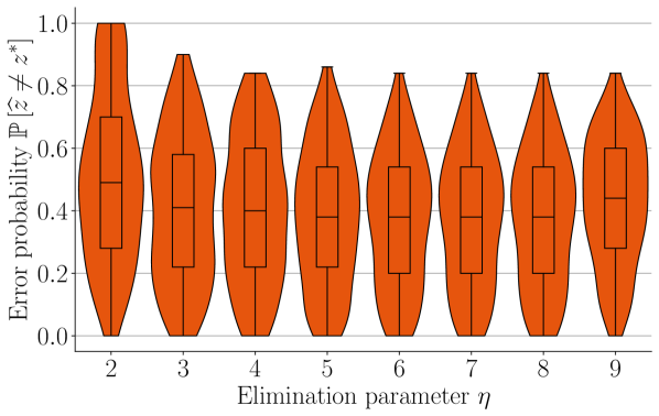
(a) $(\lambda_{\text{trans}},\widehat{\theta}_{\text{CH,DT}})$.

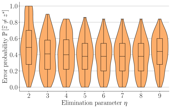
(b) $(\lambda_{\text{trans}},\widehat{\theta}_{\text{CH,}\mathbb{RT}})$.

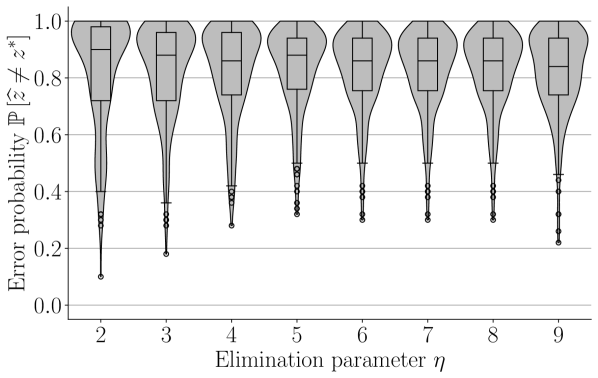
(c) $(\lambda_{\text{hard}},\widehat{\theta}_{\text{CH}})$.

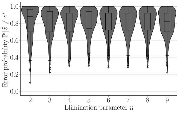
(d) $(\lambda_{\text{trans}},\widehat{\theta}_{\text{CH}})$.

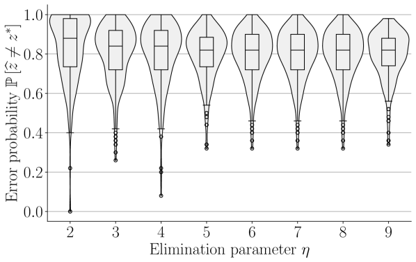
(e) $(\lambda_{\text{trans}},\widehat{\theta}_{\text{CH,logit}})$.

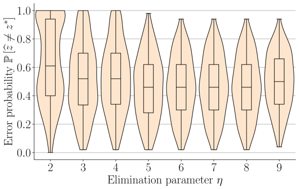
(f) $(\lambda_{\text{trans}},\widehat{\theta}_{\text{CH,DT,logit}})$.

Figure 6: Violin plots overlaid with box plots, used for tuning the elimination parameter $\eta$ in algorithm 1 for each GSE variation, simulated based on the dataset of snack preferences with yes-or-no choices [15], as discussed in section D.2. Each plot shows the best-arm identification error probability, $\mathbb{P}\left[\widehat{z}\neq z^{*}\right]$, as a function of $\eta$. The box plots follow the convention of the matplotlib Python package. The horizontal line in each box represents the median of the error probabilities across all bandit instances and budgets. Each error probability is averaged over $50$ repeated simulations under different random seeds. The top and bottom borders of the box represent the third and first quartiles, respectively, while the whiskers extend to the farthest points within $1.5\times$ the interquartile range. Flier points are the outliers past the end of the whiskers.

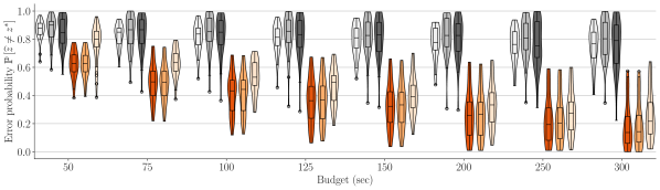
Figure 7: A violin plot overlaid with a box plot showing the best-arm identification error probability, $\mathbb{P}\left[\widehat{z}\neq z^{*}\right]$, as a function of budget for each GSE variation, simulated using the dataset of snack preferences with yes-or-no choices [15], as described in section D.2. The box plots follow the convention of the matplotlib Python package. For each GSE variation and budget, the horizontal line in the middle of the box represents the median of the error probabilities across all bandit instances. Each error probability is averaged over $300$ repeated simulations under different random seeds. The box’s upper and lower borders represent the third and first quartiles, respectively, with whiskers extending to the farthest points within $1.5\times$ the interquartile range. Flier points indicate outliers beyond the whiskers.

D.3 Processing the dataset of snack preferences with 0-or-1 choices [38]

We accessed this dataset via Fudenberg et al. [25]’s replication package at https://www.aeaweb.org/articles?id=10.1257/aer.20150742. The dataset [38] includes the choices and response times of $39$ participants, each responding to between $49$ and $100$ queries comparing two snack items. Participants’ eye movements were tracked during the experiment. The authors [38] modeled each participant’s choices, response times, and eye movements using the attentional DDM, where the drift for each query is a linear combination of the participant’s ratings of both snack items in the query, with the weights adjusting based on their eye movements. The ratings, $\in\{-10,-9,\dots,0,\dots,9,10\}$, were collected before the participants interacted with the binary queries.

In our work, if we had followed the data processing procedure for the food-gamble dataset as outlined in section D.1, each snack item’s feature vector would be encoded as a $1$-dimensional vector representing the participant’s rating. This would result in trivial bandit problems. To avoid this, we instead define the feature vector for each snack item (arm) with a participant rating $r_{z}\in\{-10,-9,\dots,0,\dots,9,10\}$ as a one-hot vector in $\mathbb{R}^{21}$, where the $(r_{z}+11)$-th element is $1$ and the rest are $0$. The preference vector $\theta^{*}$ is defined as $\beta^{*}\cdot[-10,-9,\dots,0,\dots,9,10]^{\top}\in\mathbb{R}^{21}$, where $\beta^{*}$ is participant-specific and unknown to the learner. Thus, for each arm $z$, the participant’s utility is given by $u_{z}\coloneqq z^{\top}\theta^{*}=r_{z}\beta^{*}$. This setup ensures that each participant’s data generates a bandit instance with a preference vector $\theta^{*}\in\mathbb{R}^{21}$, a set of arms $\mathcal{Z}\subset\mathbb{R}^{21}$ with $\left|\mathcal{Z}\right|=21$, and a query set $\mathcal{X}\coloneqq\left\{z-z^{\prime}\colon z\in\mathcal{Z}\right\}$. Since our focus is not on human attention or eye movements, we fit each participant’s data to our dEZDM model using Bayesian inference with non-informative priors [16]. This allowed us to identify the preference vector $\theta^{*}$ (or equivalently, the parameter $\beta^{*}$), non-decision time $t_{\text{nondec}}$, and barrier $a$. Across participants, the barrier $a$ ranged from $0.75$ to $2.192$ with a mean of $1.335$, and $t_{\text{nondec}}$ ranged from $0.387$ to $1.22$ seconds with a mean of $0.641$ seconds.

For each of the following GSE variations (introduced in section 5.2): $(\lambda_{\text{trans}},\widehat{\theta}_{\text{CH,DT}})$, $(\lambda_{\text{trans}},\widehat{\theta}_{\text{CH,}\mathbb{RT}})$, $(\lambda_{\text{trans}},\widehat{\theta}_{\text{CH}})$, $(\lambda_{\text{hard}},\widehat{\theta}_{\text{CH}})$, $(\lambda_{\text{trans}},\widehat{\theta}_{\text{CH,logit}})$, and $(\lambda_{\text{trans}},\widehat{\theta}_{\text{CH,DT,logit}})$, we tuned the elimination parameter $\eta$ in algorithm 1 using the following procedure: We considered $\eta\in\{2,3,4,5,6,7,8,9,10,11\}$, which resulted in the number of phases $\coloneqq\left\lceil\log_{\eta}|\mathcal{Z}|\right\rceil=\left\lceil\log_{\eta}(17)\right\rceil$ (3 of algorithm 1) being $\{5,3,3,2,2,2,2,2,2,2\}$, respectively. We excluded cases where $\eta>\left\lceil 21/2\right\rceil=11$, as these result in $2$ phases, identical to when $\eta\in\{5,6,7,8,9,10,11\}$. Then, for each $\eta$, for each of the 39 bandit instances, and for each budget $\in\left\{150,200,250,300,350,400,450,500\right\}$ seconds, we ran $50$ repeated simulations per GSE variation under different random seeds, sampling human feedback from the identified dEZDM. We then aggregated the results into a single best-arm identification error probability for each GSE variation, $\eta$, bandit instance, and budget. These error probabilities were compiled into violin and box plots, as shown in fig. 8.

For each GSE variation, we selected the $\eta$ that minimized the median error probability, as shown in the box plots in fig. 8. If multiple $\eta$ values yielded the same median, we used the third quartile, and if necessary, the first quartile, to break ties. Based on this approach, we selected: $\eta=4$ for $(\lambda_{\text{trans}},\widehat{\theta}_{\text{CH,DT}})$, $\eta=4$ for $(\lambda_{\text{trans}},\widehat{\theta}_{\text{CH,}\mathbb{RT}})$, $\eta=4$ for $(\lambda_{\text{trans}},\widehat{\theta}_{\text{CH}})$, $\eta=2$ for $(\lambda_{\text{hard}},\widehat{\theta}_{\text{CH}})$, $\eta=5$ for $(\lambda_{\text{trans}},\widehat{\theta}_{\text{CH,logit}})$, and $\eta=5$ for $(\lambda_{\text{trans}},\widehat{\theta}_{\text{CH,DT,logit}})$.

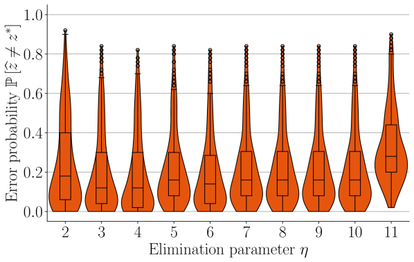
(a) $(\lambda_{\text{trans}},\widehat{\theta}_{\text{CH,DT}})$.

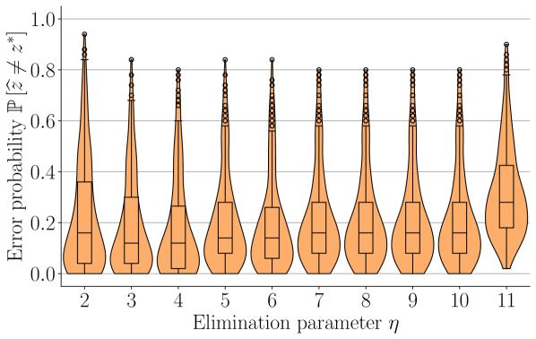
(b) $(\lambda_{\text{trans}},\widehat{\theta}_{\text{CH,}\mathbb{RT}})$.

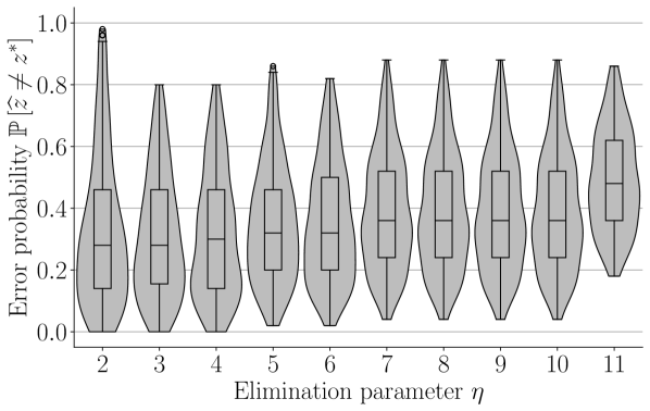
(c) $(\lambda_{\text{hard}},\widehat{\theta}_{\text{CH}})$.

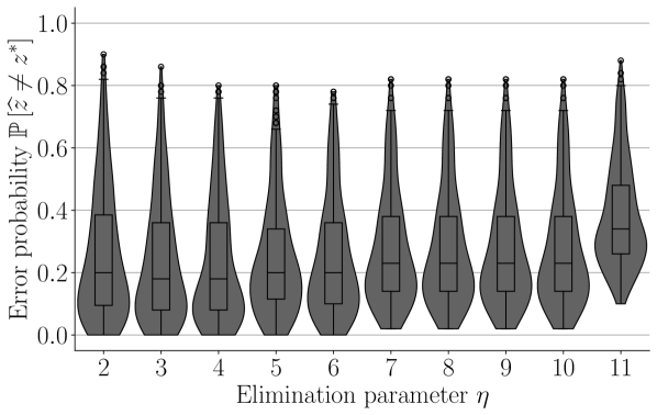
(d) $(\lambda_{\text{trans}},\widehat{\theta}_{\text{CH}})$.

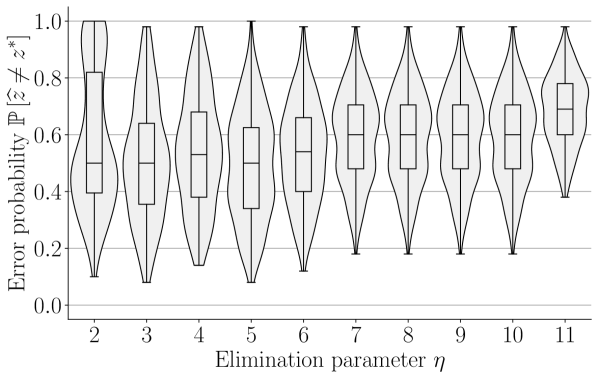
(e) $(\lambda_{\text{trans}},\widehat{\theta}_{\text{CH,logit}})$.

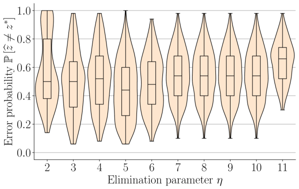
(f) $(\lambda_{\text{trans}},\widehat{\theta}_{\text{CH,DT,logit}})$.

Figure 8: Violin plots overlaid with box plots, used for tuning the elimination parameter $\eta$ in algorithm 1 for each GSE variation, simulated based on the dataset of snack preferences with $0$-or-$1$ choices [38], as discussed in section D.3. Each plot shows the best-arm identification error probability, $\mathbb{P}\left[\widehat{z}\neq z^{*}\right]$, as a function of $\eta$. The box plots follow the convention of the matplotlib Python package. The horizontal line in each box represents the median of the error probabilities across all bandit instances and budgets. Each error probability is averaged over $50$ repeated simulations under different random seeds. The top and bottom borders of the box represent the third and first quartiles, respectively, while the whiskers extend to the farthest points within $1.5\times$ the interquartile range. Flier points are the outliers past the end of the whiskers.

With the tuned elimination parameter $\eta$, we benchmarked each GSE variation on all $39$ bandit instances using its own manually tuned $\eta$. Each variation was evaluated over $300$ repeated simulations with different random seeds, where human choices and response times were sampled from the dEZDM with the identified parameters. The full results are shown in fig. 9, with selected results presented in fig. 4(c).

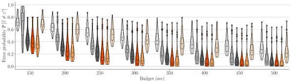
Figure 9: A violin plot overlaid with a box plot showing the best-arm identification error probability, $\mathbb{P}\left[\widehat{z}\neq z^{*}\right]$, as a function of budget for each GSE variation, simulated using the dataset of snack preferences with $0$-or-$1$ choices [38], as described in section D.3. The box plots follow the convention of the matplotlib Python package. For each GSE variation and budget, the horizontal line in the middle of the box represents the median of the error probabilities across all bandit instances. Each error probability is averaged over $300$ repeated simulations under different random seeds. The box’s upper and lower borders represent the third and first quartiles, respectively, with whiskers extending to the farthest points within $1.5\times$ the interquartile range. Flier points indicate outliers beyond the whiskers.

References

- Agrawal et al. [2019] S. Agrawal, V. Avadhanula, V. Goyal, and A. Zeevi. Mnl-bandit: A dynamic learning approach to assortment selection. Operations Research, 67(5):1453–1485, 2019. doi: 10.1287/opre.2018.1832. URL https://doi.org/10.1287/opre.2018.1832.
- Alieva et al. [2021] A. Alieva, A. Cutkosky, and A. Das. Robust pure exploration in linear bandits with limited budget. In M. Meila and T. Zhang, editors, Proceedings of the 38th International Conference on Machine Learning, volume 139 of Proceedings of Machine Learning Research, pages 187–195. PMLR, 18–24 Jul 2021. URL https://proceedings.mlr.press/v139/alieva21a.html.
- Alós-Ferrer et al. [2021] C. Alós-Ferrer, E. Fehr, and N. Netzer. Time will tell: Recovering preferences when choices are noisy. Journal of Political Economy, 129(6):1828–1877, 2021. doi: 10.1086/713732. URL https://doi.org/10.1086/713732.
- Azizi et al. [2022] M. Azizi, B. Kveton, and M. Ghavamzadeh. Fixed-budget best-arm identification in structured bandits. In L. D. Raedt, editor, Proceedings of the Thirty-First International Joint Conference on Artificial Intelligence, IJCAI-22, pages 2798–2804. International Joint Conferences on Artificial Intelligence Organization, 7 2022. doi: 10.24963/ijcai.2022/388. URL https://doi.org/10.24963/ijcai.2022/388. Main Track.
- Badanidiyuru et al. [2018] A. Badanidiyuru, R. Kleinberg, and A. Slivkins. Bandits with knapsacks. Journal of the ACM (JACM), 65(3):1–55, 2018.
- Bai et al. [2022] Y. Bai, A. Jones, K. Ndousse, A. Askell, A. Chen, N. DasSarma, D. Drain, S. Fort, D. Ganguli, T. Henighan, N. Joseph, S. Kadavath, J. Kernion, T. Conerly, S. El-Showk, N. Elhage, Z. Hatfield-Dodds, D. Hernandez, T. Hume, S. Johnston, S. Kravec, L. Lovitt, N. Nanda, C. Olsson, D. Amodei, T. Brown, J. Clark, S. McCandlish, C. Olah, B. Mann, and J. Kaplan. Training a helpful and harmless assistant with reinforcement learning from human feedback, 2022. URL https://arxiv.org/abs/2204.05862.
- Baldassi et al. [2020] C. Baldassi, S. Cerreia-Vioglio, F. Maccheroni, M. Marinacci, and M. Pirazzini. A behavioral characterization of the drift diffusion model and its multialternative extension for choice under time pressure. Management Science, 66(11):5075–5093, 2020. doi: 10.1287/mnsc.2019.3475. URL https://doi.org/10.1287/mnsc.2019.3475.
- Bengs et al. [2021] V. Bengs, R. Busa-Fekete, A. E. Mesaoudi-Paul, and E. Hüllermeier. Preference-based online learning with dueling bandits: A survey. Journal of Machine Learning Research, 22(7):1–108, 2021. URL http://jmlr.org/papers/v22/18-546.html.
- Berlinghieri et al. [2023] R. Berlinghieri, I. Krajbich, F. Maccheroni, M. Marinacci, and M. Pirazzini. Measuring utility with diffusion models. Science Advances, 9(34):eadf1665, 2023. doi: 10.1126/sciadv.adf1665. URL https://www.science.org/doi/abs/10.1126/sciadv.adf1665.
- Bogina et al. [2023] V. Bogina, T. Kuflik, D. Jannach, M. Bielikova, M. Kompan, and C. Trattner. Considering temporal aspects in recommender systems: a survey. User Modeling and User-Adapted Interaction, 33(1):81–119, 2023. doi: 10.1007/s11257-022-09335-w. URL https://doi.org/10.1007/s11257-022-09335-w.
- Brown and Heathcote [2005] S. Brown and A. Heathcote. A ballistic model of choice response time. Psychological review, 112(1):117, 2005.
- Brown and Heathcote [2008] S. D. Brown and A. Heathcote. The simplest complete model of choice response time: Linear ballistic accumulation. Cognitive Psychology, 57(3):153–178, 2008. ISSN 0010-0285. doi: https://doi.org/10.1016/j.cogpsych.2007.12.002. URL https://www.sciencedirect.com/science/article/pii/S0010028507000722.
- Castro et al. [2019] S. C. Castro, D. L. Strayer, D. Matzke, and A. Heathcote. Cognitive workload measurement and modeling under divided attention. Journal of experimental psychology: human perception and performance, 45(6):826, 2019.
- Chu et al. [2011] W. Chu, L. Li, L. Reyzin, and R. Schapire. Contextual bandits with linear payoff functions. In G. Gordon, D. Dunson, and M. Dudík, editors, Proceedings of the Fourteenth International Conference on Artificial Intelligence and Statistics, volume 15 of Proceedings of Machine Learning Research, pages 208–214, Fort Lauderdale, FL, USA, 11–13 Apr 2011. PMLR. URL https://proceedings.mlr.press/v15/chu11a.html.
- Clithero [2018a] J. A. Clithero. Improving out-of-sample predictions using response times and a model of the decision process. Journal of Economic Behavior & Organization, 148:344–375, 2018a. ISSN 0167-2681. doi: https://doi.org/10.1016/j.jebo.2018.02.007. URL https://www.sciencedirect.com/science/article/pii/S0167268118300398.
- Clithero [2018b] J. A. Clithero. Response times in economics: Looking through the lens of sequential sampling models. Journal of Economic Psychology, 69:61–86, 2018b. ISSN 0167-4870. doi: https://doi.org/10.1016/j.joep.2018.09.008. URL https://www.sciencedirect.com/science/article/pii/S0167487016306444.
- Cox [2017] D. R. Cox. Stochastic Choice Theory, Econometric Society Monograph. Routledge, 2017.
- De Boeck and Jeon [2019] P. De Boeck and M. Jeon. An overview of models for response times and processes in cognitive tests. Frontiers in Psychology, 10, 2019. ISSN 1664-1078. doi: 10.3389/fpsyg.2019.00102. URL https://www.frontiersin.org/journals/psychology/articles/10.3389/fpsyg.2019.00102.
- Degenne et al. [2020] R. Degenne, P. Menard, X. Shang, and M. Valko. Gamification of pure exploration for linear bandits. In H. D. III and A. Singh, editors, Proceedings of the 37th International Conference on Machine Learning, volume 119 of Proceedings of Machine Learning Research, pages 2432–2442. PMLR, 13–18 Jul 2020. URL https://proceedings.mlr.press/v119/degenne20a.html.
- Deldjoo et al. [2024] Y. Deldjoo, M. Schedl, and P. Knees. Content-driven music recommendation: Evolution, state of the art, and challenges. Computer Science Review, 51:100618, 2024. ISSN 1574-0137. doi: https://doi.org/10.1016/j.cosrev.2024.100618. URL https://www.sciencedirect.com/science/article/pii/S1574013724000029.
- Drugowitsch [2016] J. Drugowitsch. Fast and accurate monte carlo sampling of first-passage times from wiener diffusion models. Scientific reports, 6(1):20490, 2016.
- Fiez et al. [2019] T. Fiez, L. Jain, K. G. Jamieson, and L. Ratliff. Sequential experimental design for transductive linear bandits. In H. Wallach, H. Larochelle, A. Beygelzimer, F. d'Alché-Buc, E. Fox, and R. Garnett, editors, Advances in Neural Information Processing Systems, volume 32. Curran Associates, Inc., 2019. URL https://proceedings.neurips.cc/paper%5Ffiles/paper/2019/file/8ba6c657b03fc7c8dd4dff8e45defcd2-Paper.pdf.
- Filippi et al. [2010] S. Filippi, O. Cappe, A. Garivier, and C. Szepesvári. Parametric bandits: The generalized linear case. In J. Lafferty, C. Williams, J. Shawe-Taylor, R. Zemel, and A. Culotta, editors, Advances in Neural Information Processing Systems, volume 23. Curran Associates, Inc., 2010. URL https://proceedings.neurips.cc/paper%5Ffiles/paper/2010/file/c2626d850c80ea07e7511bbae4c76f4b-Paper.pdf.
- Fisher [2017] G. Fisher. An attentional drift diffusion model over binary-attribute choice. Cognition, 168:34–45, 2017. ISSN 0010-0277. doi: https://doi.org/10.1016/j.cognition.2017.06.007. URL https://www.sciencedirect.com/science/article/pii/S0010027717301695.
- Fudenberg et al. [2018] D. Fudenberg, P. Strack, and T. Strzalecki. Speed, accuracy, and the optimal timing of choices. American Economic Review, 108(12):3651–84, December 2018. doi: 10.1257/aer.20150742. URL https://www.aeaweb.org/articles?id=10.1257/aer.20150742.
- Fudenberg et al. [2020] D. Fudenberg, W. Newey, P. Strack, and T. Strzalecki. Testing the drift-diffusion model. Proceedings of the National Academy of Sciences, 117(52):33141–33148, 2020. doi: 10.1073/pnas.2011446117. URL https://www.pnas.org/doi/abs/10.1073/pnas.2011446117.
- Gabillon [2014] V. Gabillon. Budgeted Classification-based Policy Iteration. Theses, Universite Lille 1, June 2014. URL https://theses.hal.science/tel-01297386.
- Gourieroux and Monfort [1981] C. Gourieroux and A. Monfort. Asymptotic properties of the maximum likelihood estimator in dichotomous logit models. Journal of Econometrics, 17(1):83–97, 1981. ISSN 0304-4076. doi: https://doi.org/10.1016/0304-4076(81)90060-9. URL https://www.sciencedirect.com/science/article/pii/0304407681900609.
- Grasman et al. [2009] R. P. Grasman, E.-J. Wagenmakers, and H. L. van der Maas. On the mean and variance of response times under the diffusion model with an application to parameter estimation. Journal of Mathematical Psychology, 53(2):55–68, 2009. ISSN 0022-2496. doi: https://doi.org/10.1016/j.jmp.2009.01.006. URL https://www.sciencedirect.com/science/article/pii/S0022249609000066.
- Jun et al. [2021] K.-S. Jun, L. Jain, B. Mason, and H. Nassif. Improved confidence bounds for the linear logistic model and applications to bandits. In M. Meila and T. Zhang, editors, Proceedings of the 38th International Conference on Machine Learning, volume 139 of Proceedings of Machine Learning Research, pages 5148–5157. PMLR, 18–24 Jul 2021. URL https://proceedings.mlr.press/v139/jun21a.html.
- Karimi et al. [2018] M. Karimi, D. Jannach, and M. Jugovac. News recommender systems – survey and roads ahead. Information Processing & Management, 54(6):1203–1227, 2018. ISSN 0306-4573. doi: https://doi.org/10.1016/j.ipm.2018.04.008. URL https://www.sciencedirect.com/science/article/pii/S030645731730153X.
- Karpov and Zhang [2022] N. Karpov and Q. Zhang. Instance-sensitive algorithms for pure exploration in multinomial logit bandit. Proceedings of the AAAI Conference on Artificial Intelligence, 36(7):7096–7103, Jun. 2022. doi: 10.1609/aaai.v36i7.20669. URL https://ojs.aaai.org/index.php/AAAI/article/view/20669.
- Kaufmann et al. [2016] E. Kaufmann, O. Cappé, and A. Garivier. On the complexity of best-arm identification in multi-armed bandit models. Journal of Machine Learning Research, 17(1):1–42, 2016. URL http://jmlr.org/papers/v17/kaufman16a.html.
- Konovalov and Krajbich [2019] A. Konovalov and I. Krajbich. Revealed strength of preference: Inference from response times. Judgment and Decision Making, 14(4):381–394, 2019. doi: 10.1017/S1930297500006082.
- Koppol et al. [2020] P. Koppol, H. Admoni, and R. Simmons. Iterative interactive reward learning. In Participatory Approaches to Machine Learning, International Conference on Machine Learning Workshop, 2020.
- Koppol et al. [2021] P. Koppol, H. Admoni, and R. Simmons. Interaction considerations in learning from humans. In Z.-H. Zhou, editor, Proceedings of the Thirtieth International Joint Conference on Artificial Intelligence, IJCAI-21, pages 283–291. International Joint Conferences on Artificial Intelligence Organization, 8 2021. doi: 10.24963/ijcai.2021/40. URL https://doi.org/10.24963/ijcai.2021/40. Main Track.
- Krajbich [2019] I. Krajbich. Accounting for attention in sequential sampling models of decision making. Current Opinion in Psychology, 29:6–11, 2019. ISSN 2352-250X. doi: https://doi.org/10.1016/j.copsyc.2018.10.008. URL https://www.sciencedirect.com/science/article/pii/S2352250X18301866. Attention & Perception.
- Krajbich et al. [2010] I. Krajbich, C. Armel, and A. Rangel. Visual fixations and the computation and comparison of value in simple choice. Nature Neuroscience, 13(10):1292–1298, 2010. doi: 10.1038/nn.2635. URL https://doi.org/10.1038/nn.2635.
- Lerche et al. [2017] V. Lerche, A. Voss, and M. Nagler. How many trials are required for parameter estimation in diffusion modeling? a comparison of different optimization criteria. Behavior Research Methods, 49(2):513–537, 2017. doi: 10.3758/s13428-016-0740-2. URL https://doi.org/10.3758/s13428-016-0740-2.
- Li et al. [2010] L. Li, W. Chu, J. Langford, and R. E. Schapire. A contextual-bandit approach to personalized news article recommendation. In Proceedings of the 19th International Conference on World Wide Web, WWW ’10, page 661–670, New York, NY, USA, 2010. Association for Computing Machinery. ISBN 9781605587998. doi: 10.1145/1772690.1772758. URL https://doi.org/10.1145/1772690.1772758.
- Li et al. [2024] Z. Li, K. Jamieson, and L. Jain. Optimal exploration is no harder than Thompson sampling. In S. Dasgupta, S. Mandt, and Y. Li, editors, Proceedings of The 27th International Conference on Artificial Intelligence and Statistics, volume 238 of Proceedings of Machine Learning Research, pages 1684–1692. PMLR, 02–04 May 2024. URL https://proceedings.mlr.press/v238/li24h.html.
- McFadden [1984] D. L. McFadden. Chapter 24 Econometric analysis of qualitative response models, volume 2 of Handbook of Econometrics. Elsevier, 1984. doi: https://doi.org/10.1016/S1573-4412(84)02016-X. URL https://www.sciencedirect.com/science/article/pii/S157344128402016X.
- Menick et al. [2022] J. Menick, M. Trebacz, V. Mikulik, J. Aslanides, F. Song, M. Chadwick, M. Glaese, S. Young, L. Campbell-Gillingham, G. Irving, et al. Teaching language models to support answers with verified quotes. arXiv preprint arXiv:2203.11147, 2022.
- Minka [2003] T. P. Minka. A comparison of numerical optimizers for logistic regression. Unpublished draft, 2003. URL https://tminka.github.io/papers/logreg/minka-logreg.pdf.
- Myers et al. [2022] C. E. Myers, A. Interian, and A. A. Moustafa. A practical introduction to using the drift diffusion model of decision-making in cognitive psychology, neuroscience, and health sciences. Frontiers in Psychology, 13, 2022. ISSN 1664-1078. doi: 10.3389/fpsyg.2022.1039172. URL https://www.frontiersin.org/journals/psychology/articles/10.3389/fpsyg.2022.1039172.
- Nakano et al. [2021] R. Nakano, J. Hilton, S. Balaji, J. Wu, L. Ouyang, C. Kim, C. Hesse, S. Jain, V. Kosaraju, W. Saunders, et al. Webgpt: Browser-assisted question-answering with human feedback. arXiv preprint arXiv:2112.09332, 2021.
- Ouyang et al. [2022] L. Ouyang, J. Wu, X. Jiang, D. Almeida, C. Wainwright, P. Mishkin, C. Zhang, S. Agarwal, K. Slama, A. Ray, J. Schulman, J. Hilton, F. Kelton, L. Miller, M. Simens, A. Askell, P. Welinder, P. F. Christiano, J. Leike, and R. Lowe. Training language models to follow instructions with human feedback. In S. Koyejo, S. Mohamed, A. Agarwal, D. Belgrave, K. Cho, and A. Oh, editors, Advances in Neural Information Processing Systems, volume 35, pages 27730–27744. Curran Associates, Inc., 2022. URL https://proceedings.neurips.cc/paper%5Ffiles/paper/2022/file/b1efde53be364a73914f58805a001731-Paper-Conference.pdf.
- Palmer et al. [2005] J. Palmer, A. C. Huk, and M. N. Shadlen. The effect of stimulus strength on the speed and accuracy of a perceptual decision. Journal of Vision, 5(5):1–1, 05 2005. ISSN 1534-7362. doi: 10.1167/5.5.1. URL https://doi.org/10.1167/5.5.1.
- Pedersen et al. [2017] M. L. Pedersen, M. J. Frank, and G. Biele. The drift diffusion model as the choice rule in reinforcement learning. Psychonomic Bulletin & Review, 24(4):1234–1251, 2017. doi: 10.3758/s13423-016-1199-y. URL https://doi.org/10.3758/s13423-016-1199-y.
- Pérez-Ortiz et al. [2020] M. Pérez-Ortiz, A. Mikhailiuk, E. Zerman, V. Hulusic, G. Valenzise, and R. K. Mantiuk. From pairwise comparisons and rating to a unified quality scale. IEEE Transactions on Image Processing, 29:1139–1151, 2020. doi: 10.1109/TIP.2019.2936103.
- Ratcliff and McKoon [2008] R. Ratcliff and G. McKoon. The Diffusion Decision Model: Theory and Data for Two-Choice Decision Tasks. Neural Computation, 20(4):873–922, 04 2008. ISSN 0899-7667. doi: 10.1162/neco.2008.12-06-420. URL https://doi.org/10.1162/neco.2008.12-06-420.
- Ratcliff and Tuerlinckx [2002] R. Ratcliff and F. Tuerlinckx. Estimating parameters of the diffusion model: Approaches to dealing with contaminant reaction times and parameter variability. Psychonomic Bulletin & Review, 9(3):438–481, 2002. doi: 10.3758/BF03196302. URL https://doi.org/10.3758/BF03196302.
- Ratcliff et al. [2016] R. Ratcliff, P. L. Smith, S. D. Brown, and G. McKoon. Diffusion decision model: Current issues and history. Trends in Cognitive Sciences, 20(4):260–281, 2016. ISSN 1364-6613. doi: https://doi.org/10.1016/j.tics.2016.01.007. URL https://www.sciencedirect.com/science/article/pii/S1364661316000255.
- Rusmevichientong et al. [2014] P. Rusmevichientong, D. Shmoys, C. Tong, and H. Topaloglu. Assortment optimization under the multinomial logit model with random choice parameters. Production and Operations Management, 23(11):2023–2039, 2014. doi: https://doi.org/10.1111/poms.12191. URL https://onlinelibrary.wiley.com/doi/abs/10.1111/poms.12191.
- Sadigh et al. [2017] D. Sadigh, A. Dragan, S. Sastry, and S. Seshia. Active preference-based learning of reward functions. In Proceedings of Robotics: Science and Systems, Cambridge, Massachusetts, July 2017. doi: 10.15607/RSS.2017.XIII.053.
- Shvartsman et al. [2024] M. Shvartsman, B. Letham, E. Bakshy, and S. L. Keeley. Response time improves gaussian process models for perception and preferences. In The 40th Conference on Uncertainty in Artificial Intelligence, 2024.
- Silva et al. [2022] N. Silva, H. Werneck, T. Silva, A. C. Pereira, and L. Rocha. Multi-armed bandits in recommendation systems: A survey of the state-of-the-art and future directions. Expert Systems with Applications, 197:116669, 2022. ISSN 0957-4174. doi: https://doi.org/10.1016/j.eswa.2022.116669. URL https://www.sciencedirect.com/science/article/pii/S0957417422001543.
- Smith and Krajbich [2018] S. M. Smith and I. Krajbich. Attention and choice across domains. Journal of Experimental Psychology: General, 147(12):1810, 2018.
- Somers et al. [2017] T. Somers, N. R. Lawrance, and G. A. Hollinger. Efficient learning of trajectory preferences using combined ratings and rankings. In Robotics: Science and Systems Conference Workshop on Mathematical Models, Algorithms, and Human-Robot Interaction, 2017.
- Stiennon et al. [2020] N. Stiennon, L. Ouyang, J. Wu, D. Ziegler, R. Lowe, C. Voss, A. Radford, D. Amodei, and P. F. Christiano. Learning to summarize with human feedback. In H. Larochelle, M. Ranzato, R. Hadsell, M. Balcan, and H. Lin, editors, Advances in Neural Information Processing Systems, volume 33, pages 3008–3021. Curran Associates, Inc., 2020. URL https://proceedings.neurips.cc/paper%5Ffiles/paper/2020/file/1f89885d556929e98d3ef9b86448f951-Paper.pdf.
- Strzalecki [2024] T. Strzalecki. The theory of stochastic processes. Cambridge University Press, 2024. URL https://scholar.harvard.edu/sites/scholar.harvard.edu/files/tomasz/files/manuscript%5F01.pdf.
- Tao et al. [2018] C. Tao, S. Blanco, and Y. Zhou. Best arm identification in linear bandits with linear dimension dependency. In J. Dy and A. Krause, editors, Proceedings of the 35th International Conference on Machine Learning, volume 80 of Proceedings of Machine Learning Research, pages 4877–4886. PMLR, 10–15 Jul 2018. URL https://proceedings.mlr.press/v80/tao18a.html.
- Thomas et al. [2019] A. W. Thomas, F. Molter, I. Krajbich, H. R. Heekeren, and P. N. C. Mohr. Gaze bias differences capture individual choice behaviour. Nature Human Behaviour, 3(6):625–635, 2019. doi: 10.1038/s41562-019-0584-8. URL https://doi.org/10.1038/s41562-019-0584-8.
- Tirinzoni and Degenne [2022] A. Tirinzoni and R. Degenne. On elimination strategies for bandit fixed-confidence identification. In S. Koyejo, S. Mohamed, A. Agarwal, D. Belgrave, K. Cho, and A. Oh, editors, Advances in Neural Information Processing Systems, volume 35, pages 18586–18598. Curran Associates, Inc., 2022. URL https://proceedings.neurips.cc/paper%5Ffiles/paper/2022/file/760564ebba4797d0dcf1678e96e8cbcb-Paper-Conference.pdf.
- Trueblood et al. [2014] J. S. Trueblood, S. D. Brown, and A. Heathcote. The multiattribute linear ballistic accumulator model of context effects in multialternative choice. Psychological review, 121(2):179, 2014.
- Tucker et al. [2020] M. Tucker, E. Novoseller, C. Kann, Y. Sui, Y. Yue, J. W. Burdick, and A. D. Ames. Preference-based learning for exoskeleton gait optimization. In 2020 IEEE International Conference on Robotics and Automation (ICRA), pages 2351–2357, 2020. doi: 10.1109/ICRA40945.2020.9196661.
- Usher and McClelland [2001] M. Usher and J. L. McClelland. The time course of perceptual choice: the leaky, competing accumulator model. Psychological review, 108(3):550, 2001.
- Wagenmakers et al. [2007] E.-J. Wagenmakers, H. L. J. Van Der Maas, and R. P. P. P. Grasman. An ez-diffusion model for response time and accuracy. Psychonomic Bulletin & Review, 14(1):3–22, 2007. doi: 10.3758/BF03194023. URL https://doi.org/10.3758/BF03194023.
- Wagenmakers et al. [2008] E.-J. Wagenmakers, H. L. J. van der Maas, C. V. Dolan, and R. P. P. P. Grasman. Ez does it! extensions of the ez-diffusion model. Psychonomic Bulletin & Review, 15(6):1229–1235, 2008. doi: 10.3758/PBR.15.6.1229. URL https://doi.org/10.3758/PBR.15.6.1229.
- Wainwright [2019] M. J. Wainwright. High-dimensional statistics: A non-asymptotic viewpoint, volume 48. Cambridge university press, 2019.
- Webb [2019] R. Webb. The (neural) dynamics of stochastic choice. Management Science, 65(1):230–255, 2019. doi: 10.1287/mnsc.2017.2931. URL https://doi.org/10.1287/mnsc.2017.2931.
- Wiecki et al. [2013] T. V. Wiecki, I. Sofer, and M. J. Frank. Hddm: Hierarchical bayesian estimation of the drift-diffusion model in python. Frontiers in Neuroinformatics, 7, 2013. ISSN 1662-5196. doi: 10.3389/fninf.2013.00014. URL https://www.frontiersin.org/journals/neuroinformatics/articles/10.3389/fninf.2013.00014.
- Wilde et al. [2022] N. Wilde, E. Biyik, D. Sadigh, and S. L. Smith. Learning reward functions from scale feedback. In A. Faust, D. Hsu, and G. Neumann, editors, Proceedings of the 5th Conference on Robot Learning, volume 164 of Proceedings of Machine Learning Research, pages 353–362. PMLR, 08–11 Nov 2022. URL https://proceedings.mlr.press/v164/wilde22a.html.
- Xiang Chiong et al. [2024] K. Xiang Chiong, M. Shum, R. Webb, and R. Chen. Combining choice and response time data: A drift-diffusion model of mobile advertisements. Management Science, 70(2):1238–1257, 2024. doi: 10.1287/mnsc.2023.4738. URL https://doi.org/10.1287/mnsc.2023.4738.
- Xu et al. [2017] Y. Xu, H. Zhang, K. Miller, A. Singh, and A. Dubrawski. Noise-tolerant interactive learning using pairwise comparisons. In I. Guyon, U. V. Luxburg, S. Bengio, H. Wallach, R. Fergus, S. Vishwanathan, and R. Garnett, editors, Advances in Neural Information Processing Systems, volume 30. Curran Associates, Inc., 2017. URL https://proceedings.neurips.cc/paper%5Ffiles/paper/2017/file/e11943a6031a0e6114ae69c257617980-Paper.pdf.
- Yang and Tan [2022] J. Yang and V. Tan. Minimax optimal fixed-budget best arm identification in linear bandits. In S. Koyejo, S. Mohamed, A. Agarwal, D. Belgrave, K. Cho, and A. Oh, editors, Advances in Neural Information Processing Systems, volume 35, pages 12253–12266. Curran Associates, Inc., 2022. URL https://proceedings.neurips.cc/paper%5Ffiles/paper/2022/file/4f9342b74c3bb63f6e030d8263082ab6-Paper-Conference.pdf.
- Yang and Krajbich [2023] X. Yang and I. Krajbich. A dynamic computational model of gaze and choice in multi-attribute decisions. Psychological Review, 130(1):52, 2023.
- Yu et al. [2023] H. Yu, R. M. Aronson, K. H. Allen, and E. S. Short. From “thumbs up” to “10 out of 10”: Reconsidering scalar feedback in interactive reinforcement learning. In 2023 IEEE/RSJ International Conference on Intelligent Robots and Systems (IROS), pages 4121–4128, 2023. doi: 10.1109/IROS55552.2023.10342458.
- Yue et al. [2012] Y. Yue, J. Broder, R. Kleinberg, and T. Joachims. The k-armed dueling bandits problem. Journal of Computer and System Sciences, 78(5):1538–1556, 2012. ISSN 0022-0000. doi: https://doi.org/10.1016/j.jcss.2011.12.028. URL https://www.sciencedirect.com/science/article/pii/S0022000012000281. JCSS Special Issue: Cloud Computing 2011.
- Zhang et al. [2023] C. Zhang, C. Kemp, and N. Lipovetzky. Goal recognition with timing information. Proceedings of the International Conference on Automated Planning and Scheduling, 33(1):443–451, Jul. 2023. doi: 10.1609/icaps.v33i1.27224. URL https://ojs.aaai.org/index.php/ICAPS/article/view/27224.
- Zhang et al. [2024] C. Zhang, C. Kemp, and N. Lipovetzky. Human goal recognition as bayesian inference: Investigating the impact of actions, timing, and goal solvability. In Proceedings of the 23rd International Conference on Autonomous Agents and Multiagent Systems, AAMAS ’24, page 2066–2074, Richland, SC, 2024. International Foundation for Autonomous Agents and Multiagent Systems. ISBN 9798400704864.