How to unravel the nature of the state from correlation functions
Abstract
We calculate the correlation functions for the , and states, which in the chiral unitary approach predict an excited state at the threshold, recently observed by the Belle collaboration. Once this is done, we tackle the inverse problem of seeing how much information one can obtain from these correlation functions. With the resampling method, one can determine the scattering parameters of all the channels with relative precision by means of the analysis in a general framework, and find a clear cusp-like structure corresponding to the in the different amplitudes at the threshold.
I Introduction
The states with are a benchmark for hadron spectroscopy, usually demanding for their interpretation large meson-baryon components on top of the conventional seed, when not being dominated by this meson-baryon cloud. A recent review on this topic can be found in Ref. [1]. In the present work we are concerned just about one of these states that still is controversial, a state appearing around the threshold, with mass and relatively narrow width. This state is predicted in studies of meson-baryon interaction using the chiral unitary approach, where the two states appear [2, 3], but it is quite elusive and it was missed in early investigations. A clear state as a pole in the second Riemann sheet was found in the work of Ref. [4]. This was corroborated in Ref. [5], where using a slightly different input in the same chiral unitary approach one failed to get this state when using physical masses of the states, but obtained it with masses slightly changed to be closer to the SU(3) limit of equal masses for the octet baryons and equal masses for the octet mesons. We anticipate here that while there is a drastic step between having or not having the pole, the physical magnitudes around the threshold change continuously and smoothly from one situation to the other. Whether disclosed or not, and having the state as a bound or a virtual state, all different works along the line of the chiral unitary approach produce this state and have some threshold enhancement in the scattering amplitudes of the coupled channels around the threshold in isospin [6, 7, 8, 9, 10, 11, 12]. The state around the threshold remains when the mixing of pseudoscalar-baryon and vector-baryons components is allowed [13, 14]. The data from photoproduction in [15] were considered in Ref. [16] to constrain the parameters of the theory and no pole was found in the second Riemann sheet, although a cusp-like structure appeared in for the different amplitudes at the threshold.
The situation of this state is similar to the one of the , which also appears as a clear cusp in recent experiments [17, 18, 19, 20, 21] and theoretical studies [22, 23, 24, 25, 26]. In spite of this clear situation, the is accepted as a resonance, and, correspondingly, there should not be a problem in calling resonance this state close to the threshold, a criterium that we will adopt in what follows.
Many suggestions of experiments have been done to find this elusive state. In Ref. [27] the reaction is proposed to observe this state. In Refs. [28, 29] the reaction, with and being mesons and baryons of the SU(3) octet, is also shown to be suited to the observation of this state. In Ref. [30], the authors proposed to search for the in the mass distribution of the process . A similar work was performed in Ref. [31] suggesting the , considering the contributions from the and final state interactions within the chiral unitary approach, from where the and the around threshold emerged. Also, the spectra of the Belle experiment on the reaction [32] was analyzed in Ref. [33], showing that a fit to the data improved substantially by including the contribution of a state at . In Ref. [34], the reaction was shown to be driven by a triangle singularity that reinforced the production of the state. In the same work, it was suggested to look at the reaction, where the signal should be equally seen. This reaction has been performed recently by the Belle collaboration [35] and a clear signal is seen at the threshold, both in the and mass distributions. This is the first clear evidence of the existence of this state. The authors of the work also state that from their analysis they cannot discriminate from the peak being due to a resonance or to a cusp in the threshold. It should be clear from the former discussion that we also do not make a strong difference between the two scenarios since one can pass from one to the other with a minor change in the strength of the interaction or other parameters of the theory. Yet, the nature of this state and its properties deserve further investigations. This is the purpose of the present work.
In this work, we propose to use the femtoscopic correlation functions of the coupled channels, which generate the state in the chiral unitary approach, to further reveal the origin and properties tied to the state. Thus we construct the correlation functions for the channels and , and in a second step we face the inverse problem in which, starting from these correlation functions we determine the possible existence of an state close to the threshold, and the scattering length and effective range for the different channels. While the procedure might look like a tautology, this is not the case because the information on the correlation functions, which is related to amplitudes above the threshold of the channels, is more limited than the one of the original model from where they are evaluated. Then it is important to know how much information one can get from the correlation functions and the uncertainties expected for the magnitudes determined from them assuming certain errors in the measurements of the correlation functions.
Femtoscopic correlation functions are emerging as a relevant experimental tool, showing the potential to provide information on the interaction of hadrons, scattering parameters and the nature of hadronic resonances. Experimental measurements are already available in Refs. [36, 37, 38, 39, 40, 41, 42, 43, 44, 45, 46, 47, 48, 49] and theoretical studies are also progressing at the same path [50, 51, 52, 53, 54, 55, 56, 57, 58, 59, 60, 61, 62, 63, 64, 65, 64, 66, 67, 68, 69, 70], with some later works involved in a model independent analysis of experimental data to extract the encoded information on scattering parameters and possible related bound states and resonances [71, 72, 73, 74] . In the present work, we explore the potential of using correlation functions to study the , find out about its nature, and at the same time determine scattering parameters for the related coupled channels , and .
II Formalism
II.1 Summary of the chiral unitary approach for in coupled channels
In this work, we first provide a brief introduction of the and related channels interactions within the chiral unitary approach [3]. To avoid using the Coulomb interaction, we will take the coupled channels with which only have one charged particle. The channels are , , , , and that we label respectively. For the purpose of getting the state, we can safely ignore the channel, the threshold of which is far away from . Considering the phase convention of the isopin multiplets: , , and , we can easily convert isopin states to charge states, and the relationship is given by
| (1) |
The interaction of the coupled channels is given by
| (2) |
with
| (3) |
where is the c.m. energy of the meson-baryon system, and and are the masses of the meson and baryon in channel , respectively. The coefficients of Eq. (2) are given in Table 1.
| 1 | |||||
The scattering matrix follows the Bethe-Salpeter (BS) equation in coupled channels,
| (4) |
where is a diagonal matrix with its elements being the meson-baryon loop function regularized with a cutoff. Following Ref. [22], is given by
| (5) |
with , and [3].
With this input, we obtain a pole at
| (6) |
The width is very large, but we shall discuss later the meaning of this result.
II.2 Correlation functions
Following Ref. [62], the correlation functions can be written as
| (7) |
| (8) |
| (9) |
| (10) |
| (11) |
where are the momenta of the particles in the center of mass frame,
| (12) |
is the source function, which is parameterized as a Gaussian normalized to ,
| (13) |
with being the size of the source function, which usually equals for collisions, and the function is defined as
| (14) |
with the zeroth order spherical Bessel function. We have assumed that the weights of the inelastic channels are unity, as demanded for the elastic channel. This could be different and these weights must be obtained from the experiment, but in order to see the power of the correlation functions to determine values of the observables and their uncertainties we assume these weights as unity in the direct calculation and inverse analysis.
II.3 Observables
We evaluate the scattering length and effective range for each channel using the relationship of the matrix of Eq. (4) to that in the Quantum Mechanics formalism as described in Ref. [75]. This relationship is given by
| (15) |
with
| (16) |
from which we easily find
| (17) |
| (18) |
where is the reduced mass of channel , and is the threshold energy for the channel .
II.4 Inverse problem
First, we use the bootstrap or resampling method [76, 77, 78], generating random centroids of the data with Gaussian distributed weights within the error bars of the correlation functions of the chiral unitary approach to which we associate error, typical of present correlation data. We take points from each correlation function and assume these new centroids with the same errors of . We repeat the procedure about times and attempt to extract the maximum information available by using a general framework with minimal model dependence. For the inverse problem, we assume that the general interaction has an energy dependence like Eq. (2), given by
| (19) |
and that this potential is isospin symmetric (isospin is slightly broken in the matrix due to the difference of masses between the particles in the same isopin multiplets and their effect on the loops). Actually, since we are concerned only about the peak around , the term is practically constant and we can consider the approach really model independent. Using Eq. (II.1) we can have the new symmetric coefficients shown in Table 2, where and are coefficients of and respectively. The fractional coefficients in the table indicate the component of the states according to Eq. (II.1). The matrix is given by Eq. (4), and the function from Eq. (II.1) is used with a free parameter . We would have free parameters in plus and to fit our five correlation functions.
III Considerations on the state
In the process of the resampling, we also search for possible poles of Eq. (4) in the second Riemann sheet which is obtained using instead of of Eq. (II.1) as
| (20) |
for , , . We refrain from making the change of Eq. (20) to closed channels since becomes purely imaginary and Eq. (20) increases the size of the negative function, effectively increasing the size of attractive interactions and eventually producing states. This procedure generates poles (virtual states). By adhering to Eq. (20) without altering the potential, one approaches the results obtained from solving the equivalent Schrödinger equation with a specified potential. In this equivalent Schrödinger equation, there exists a threshold strength at which a bound state will vanish if the potential is slightly reduced.
With this former caveat when we perform the resampling procedure we obtain poles, and we make the average and dispersion of the pole position and find
| (21) |
This is highly surprising since it would imply a width of about , when the width of the state is about according to the Belle experiment [35]. In Ref. [16] one does not find the pole and instead one finds a cusp at the threshold for of the different amplitudes. The result of Eq. (21) is basically consistent with that of Eq. (6), and we learn that we can obtain the pole position from the correlation functions, with an uncertainty of about in the position and around in the width, with the assumed uncertainty in the correlation functions.
The results of Eq. (6) are similar to those obtained in Ref. [4], where, as shown in Ref. [5], a pole would appear close to the threshold and with a width of the order of . However, as discussed in Ref. [5], poles found around the threshold must be taken with caution and one should note that the experiment will see amplitudes in the physical real energy axis and in that case the extrapolation to the complex plane will be very model dependent. This is actually the case here.
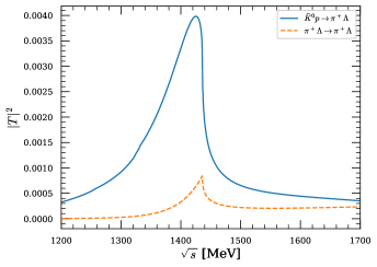
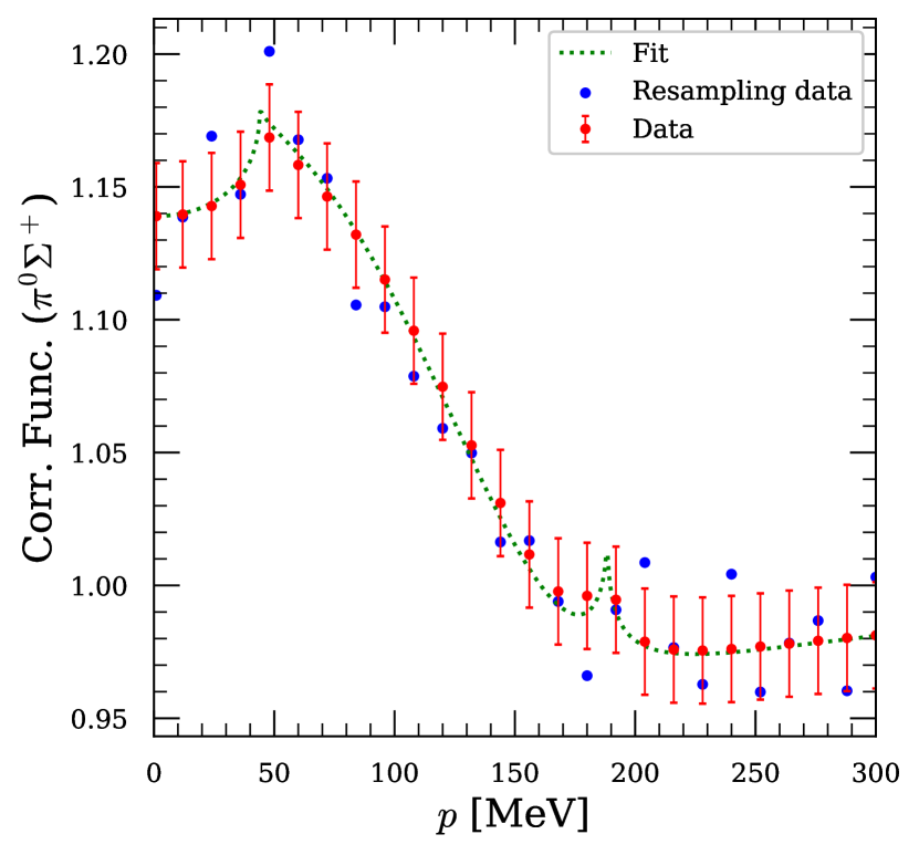
Indeed, in Fig. 1 we show results for for different amplitudes and we see that in all cases we find looking like a cusp around the threshold with an apparent width of .
It is surprising that in spite of having a pole indicating a width of about , the results of just produce a peak around the threshold with an apparent width of , as seen in the Belle experiment. This should serve as a caution when trying to interpret poles found around threshold.
It is also interesting mentioning that in the work of Ref. [16] the chiral potential was slightly modified and adjusted to the photoproduction data of Ref. [15]. This resulted in a reduction of the strength of the potentials by about a factor of the order of . In that case no pole was obtained for , but a clear cusp at threshold resulted from the different amplitudes. With this in mind, we make the exercise of reducing gradually the potential to see if the pole disappears. We find that multiplying the coefficients of Table 1 by , the pole already disappears. This represents a discontinuous transition from possessing to lacking a pole. However, it is noteworthy that the amplitudes change continuously. In Fig. 1, the alterations caused by the normalization factor of are approximately , with no apparent modifications in the shapes and widths of the structures depicted.
IV Results
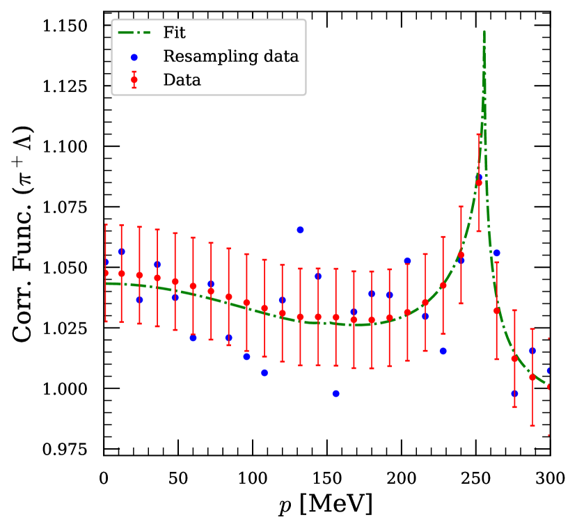
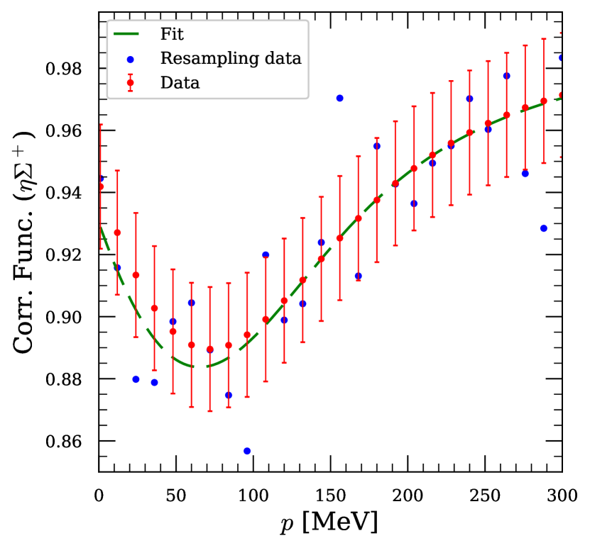
We use the chiral unitary approach in Section II with the cutoff regularization of . The scattering length and effective range for different channels are presented in Table 3 and Table 4, respectively. The results for the correlation functions of the different channels are shown in Fig 2, calculated with .
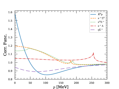
The observed cusps correspond to the opening of some channels. It is a big surprising to see effective ranges so large in the and channels. We have checked that in the channels they are related to small cusps appearing in the corresponding diagonal elements of the matrix. Such subtle threshold effects can be much model dependent and it would be good to see if they are supported by experimental studies.
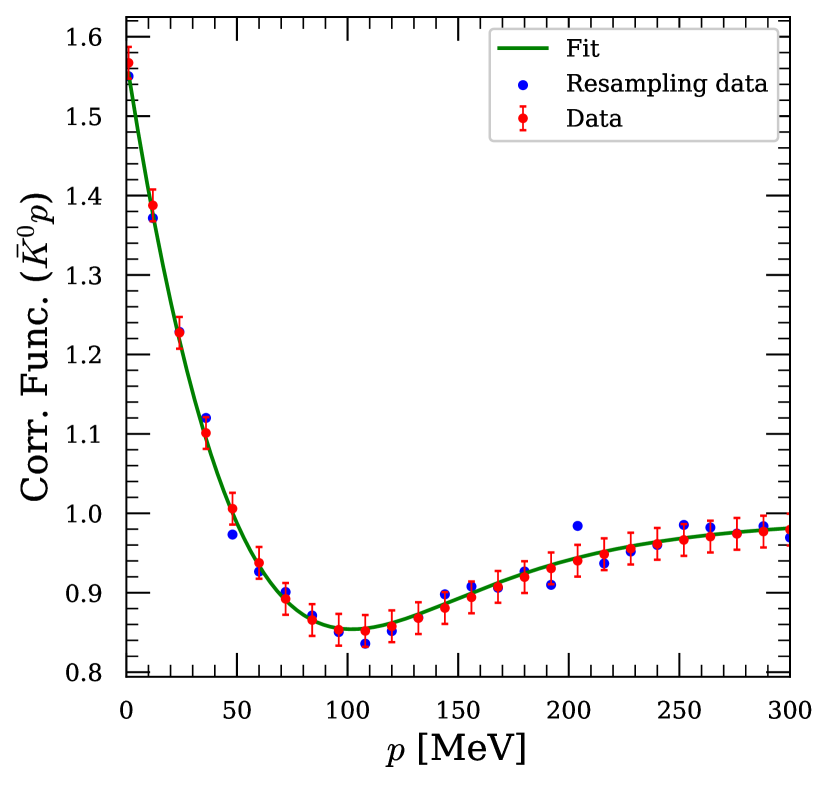
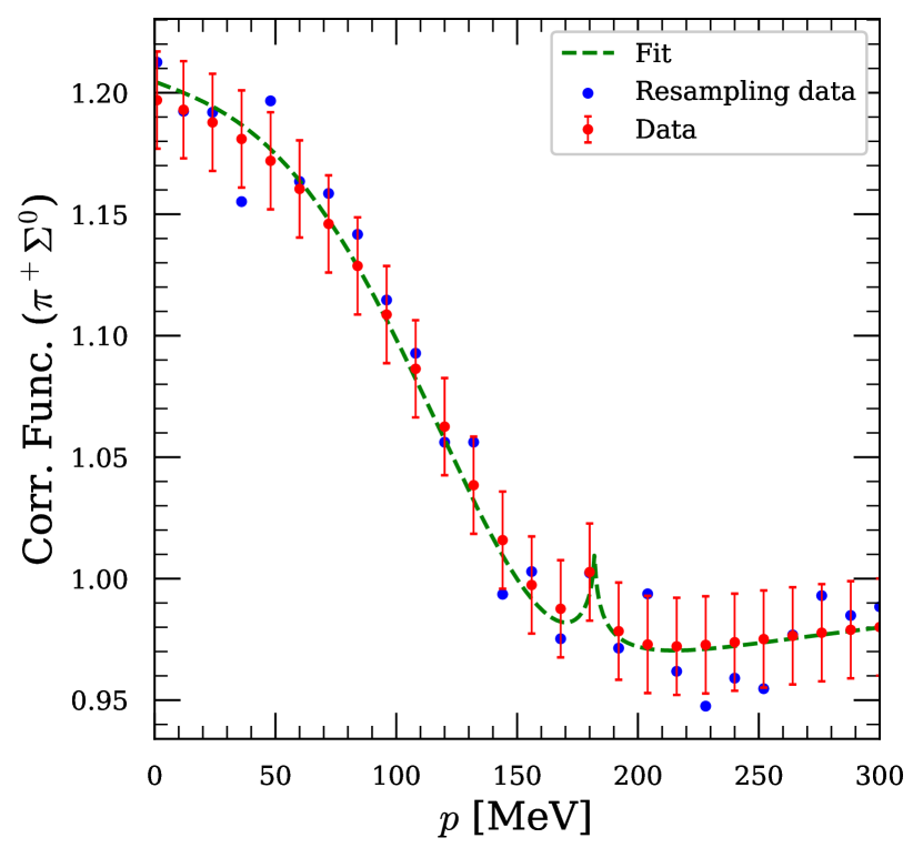
Next, we discuss the results obtained from fitting the data using the resampling method. The data with the assumed errors are shown in Fig. 3.
The average values and dispersion of the obtained parameters are shown in Table 5.
| (MeV) | (fm) | |||
The first comment is that has a high precision of around and the follows with a precision of around . The matrix elements which are zero in Table 1 are small here, but the errors in for subscripts and are not small. Other elements are compatible with Table 1 within errors, which are around except for . However, one should not pay too much attention to the values of these parameters because there are correlations among them, and different sets of parameters give rise to the same results for the observables. This means that different sets of parameters can give the same results for the observables, and this is why the uncertainties of some parameters are so large. This is the value of using the resampling method that randomly generates different equivalent sets of parameters and all that one has to do is to evaluate the average and dispersion of the observables obtained from the different fits in the resampling procedure.
The scattering lengths and effective ranges from the fit to the correlation functions are shown in Table 6 and Table 7, respectively. The scattering lengths are comparable well to the original ones, with small errors. The effective ranges are very large for the and , and so are the uncertainties obtained from the correlation functions.
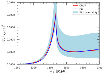
Finally, in Fig. 4, we show considering the uncertainties induced by the errors in the correlation functions. Independently on whether there is or not a pole, the correlation functions of Fig. 3 induce a cusp-like structure for the amplitude at the with the uncertainties reflected by the band of the figure.
V Conclusions
We have studied the correlation functions of the coupled channels of , , and , based on the chiral unitary approach, which produces the two states and the in , the and surprisingly a new state, a state at the threshold, which, after many attempts to be found experimentally, has been clearly observed in a recent experiment by the Belle collaboration. We discuss that the state is in the border line of being a bound state or a virtual state, but we also show that scattering amplitudes have a smooth transition from one to the other case.
In order to learn more about this state we suggest to measure correlation functions of all the channels involved. We have evaluated these correlations functions and then we tackle the inverse problem, which is to see which information we can get from the correlation functions concerning scattering parameters, and in particular, if from the correlation functions we can get evidence of the existence of this state. The answer is positive and we show that the correlation functions have encoded information leading to a clear cusp structure in at the threshold.
We study in detail the uncertainties in the observables that we determine from the correlation functions assuming errors typical of present measurements. For this we use the resampling method generating many Gaussian random sets of centroids of the correlation functions data, and carrying fits to these data with a model independent method. The uncertainties in the scattering lengths and effective ranges of the different channels are relatively small, of the order of or smaller. And the state at the threshold of can be induced from the model independent framework used to fit the correlation functions. With improved precision in the correlation data one could even distinguish between the state being a bound or a virtual state, although we also stress that this distinction has no repercussion in the observable magnitudes.
Acknowledgments
En Wang acknowledges the support from the National Key R&D Program of China (No. 2024YFE0105200). This work is partly supported by the National Natural Science Foundation of China (NSFC) under Grants No. 12365019, No. 11975083, No.12175239, No. 12221005, No. 12475086 and No. 12192263, and by the Central Government Guidance Funds for Local Scientific and Technological Development, China (No. Guike ZY22096024), the Natural Science Foundation of Guangxi province under Grant No. 2023JJA110076, and partly by the Natural Science Foundation of Changsha under Grant No. kq2208257 and the Natural Science Foundation of Hunan province under Grant No. 2023JJ30647 (CWX), and the Natural Science Foundation of Henan under Grant No. 232300421140 and No. 222300420554. This work is also partly supported by the Spanish Ministerio de Economia y Competitividad (MINECO) and European FEDER funds under Contracts No. FIS2017-84038-C2-1-P B, PID2020-112777GB-I00, and by Generalitat Valenciana under contract PROMETEO/2020/023. This project has received funding from the European Union Horizon 2020 research and innovation programme under the program H2020-INFRAIA-2018-1, grant agreement No. 824093 of the STRONG-2020 project, and by the Xiaomi Foundation / Xiaomi Young Talents Program.
References
- [1] E. Wang, L.-S. Geng, J.-J. Wu, J.-J. Xie, and B.-S. Zou, Review of the low-lying excited baryons , arXiv:2406.07839 [hep-ph] .
- Kaiser et al. [1995] N. Kaiser, P. B. Siegel, and W. Weise, Chiral dynamics and the low-energy kaon - nucleon interaction, Nucl. Phys. A 594, 325 (1995), arXiv:nucl-th/9505043 .
- Oset and Ramos [1998] E. Oset and A. Ramos, Non-perturbative chiral approach to -wave interactions, Nucl. Phys. A 635, 99 (1998), arXiv:nucl-th/9711022 .
- Oller and Meissner [2001] J. A. Oller and U. G. Meissner, Chiral dynamics in the presence of bound states: Kaon nucleon interactions revisited, Phys. Lett. B 500, 263 (2001), arXiv:hep-ph/0011146 .
- Jido et al. [2003] D. Jido, J. A. Oller, E. Oset, A. Ramos, and U. G. Meissner, Chiral dynamics of the two states, Nucl. Phys. A 725, 181 (2003), arXiv:nucl-th/0303062 .
- Oset et al. [2002] E. Oset, A. Ramos, and C. Bennhold, Low lying excited baryons and chiral symmetry, Phys. Lett. B 527, 99 (2002), [Erratum: Phys. Lett. B 530, 260–260 (2002)], arXiv:nucl-th/0109006 .
- Khemchandani et al. [2019] K. P. Khemchandani, A. Martínez Torres, and J. A. Oller, Hyperon resonances coupled to pseudoscalar- and vector-baryon channels, Phys. Rev. C 100, 015208 (2019), arXiv:1810.09990 [hep-ph] .
- Kamiya et al. [2016] Y. Kamiya, K. Miyahara, S. Ohnishi, Y. Ikeda, T. Hyodo, E. Oset, and W. Weise, Antikaon-nucleon interaction and (1405) in chiral SU(3) dynamics, Nucl. Phys. A 954, 41 (2016), arXiv:1602.08852 [hep-ph] .
- Oller [2006] J. A. Oller, On the strangeness -wave meson-baryon scattering, Eur. Phys. J. A 28, 63 (2006), arXiv:hep-ph/0603134 .
- Garcia-Recio et al. [2003] C. Garcia-Recio, J. Nieves, E. Ruiz Arriola, and M. J. Vicente Vacas, meson baryon unitarized coupled channel chiral perturbation theory and the resonances and , Phys. Rev. D 67, 076009 (2003), arXiv:hep-ph/0210311 .
- Lutz and Kolomeitsev [2002] M. F. M. Lutz and E. E. Kolomeitsev, Relativistic chiral SU(3) symmetry, large- sum rules and meson-baryon scattering, Nucl. Phys. A 700, 193 (2002), arXiv:nucl-th/0105042 .
- Guo and Oller [2013] Z.-H. Guo and J. A. Oller, Meson-baryon reactions with strangeness within a chiral framework, Phys. Rev. C 87, 035202 (2013), arXiv:1210.3485 [hep-ph] .
- Khemchandani et al. [2012] K. P. Khemchandani, A. Martinez Torres, H. Nagahiro, and A. Hosaka, Negative parity and resonances coupled to pseudoscalar and vector mesons, Phys. Rev. D 85, 114020 (2012), arXiv:1203.6711 [nucl-th] .
- Khemchandani et al. [2011] K. P. Khemchandani, A. Martinez Torres, H. Kaneko, H. Nagahiro, and A. Hosaka, Coupling vector and pseudoscalar mesons to study baryon resonances, Phys. Rev. D 84, 094018 (2011), arXiv:1107.0574 [nucl-th] .
- Moriya et al. [2013] K. Moriya et al. (CLAS), Measurement of the photoproduction line shapes near the (1405), Phys. Rev. C 87, 035206 (2013), arXiv:1301.5000 [nucl-ex] .
- Roca and Oset [2013] L. Roca and E. Oset, Isospin 0 and 1 resonances from photoproduction data, Phys. Rev. C 88, 055206 (2013), arXiv:1307.5752 [nucl-th] .
- Rubin et al. [2004] P. Rubin et al. (CLEO), First Observation and Dalitz Analysis of the Decay, Phys. Rev. Lett. 93, 111801 (2004), arXiv:hep-ex/0405011 .
- Ablikim et al. [2017] M. Ablikim et al. (BESIII), Amplitude analysis of the decays, Phys. Rev. D 95, 032002 (2017), arXiv:1610.02479 [hep-ex] .
- Chen et al. [2020] Y. Q. Chen et al. (Belle), Dalitz analysis of decays at Belle, Phys. Rev. D 102, 012002 (2020), arXiv:2003.07759 [hep-ex] .
- Ablikim et al. [2020] M. Ablikim et al. (BESIII), Measurements of Absolute Branching Fractions of Fourteen Exclusive Hadronic Decays to , Phys. Rev. Lett. 124, 241803 (2020), arXiv:2004.13910 [hep-ex] .
- Ablikim et al. [2024] M. Ablikim et al. (BESIII), Observation of in the Amplitude Analysis of , Phys. Rev. Lett. 132, 131903 (2024), arXiv:2309.05760 [hep-ex] .
- Oller et al. [1999] J. A. Oller, E. Oset, and J. R. Pelaez, Meson meson interaction in a nonperturbative chiral approach, Phys. Rev. D 59, 074001 (1999), [Erratum: Phys. Rev. D 60, 099906 (1999), Erratum: Phys. Rev. D 75, 099903 (2007)], arXiv:hep-ph/9804209 .
- Xie et al. [2015] J.-J. Xie, L.-R. Dai, and E. Oset, The low lying scalar resonances in the decays into and , , , Phys. Lett. B 742, 363 (2015), arXiv:1409.0401 [hep-ph] .
- Liang et al. [2016] W.-H. Liang, J.-J. Xie, and E. Oset, , , and production in the reaction, Eur. Phys. J. C 76, 700 (2016), arXiv:1609.03864 [hep-ph] .
- Toledo et al. [2021] G. Toledo, N. Ikeno, and E. Oset, Theoretical study of the reaction, Eur. Phys. J. C 81, 268 (2021), arXiv:2008.11312 [hep-ph] .
- Ikeno et al. [2024] N. Ikeno, J. M. Dias, W.-H. Liang, and E. Oset, reaction and , Eur. Phys. J. C 84, 469 (2024), arXiv:2402.04073 [hep-ph] .
- Lyu et al. [2023] Y.-H. Lyu, H. Zhang, N.-C. Wei, B.-C. Ke, E. Wang, and J.-J. Xie, Photo-production of lowest state within the Regge-effective Lagrangian approach, Chin. Phys. C 47, 053108 (2023), arXiv:2301.08615 [hep-ph] .
- Ren et al. [2015] X.-L. Ren, E. Oset, L. Alvarez-Ruso, and M. J. Vicente Vacas, Antineutrino induced (1405) production off the proton, Phys. Rev. C 91, 045201 (2015), arXiv:1501.04073 [hep-ph] .
- Wu and Zou [2015] J.-J. Wu and B.-S. Zou, Hyperon Production from Neutrino–Nucleon Reaction, Few Body Syst. 56, 165 (2015), arXiv:1307.0574 [hep-ph] .
- Wang et al. [2016] E. Wang, J.-J. Xie, and E. Oset, decay into in search of an , baryon state around threshold, Phys. Lett. B 753, 526 (2016), arXiv:1509.03367 [hep-ph] .
- Liu et al. [2018] L.-J. Liu, E. Wang, J.-J. Xie, K.-L. Song, and J.-Y. Zhu, production in the process , Phys. Rev. D 98, 114017 (2018), arXiv:1712.07469 [hep-ph] .
- Li et al. [2023] L. K. Li et al. (Belle), Measurement of branching fractions of and at Belle, Phys. Rev. D 107, 032004 (2023), arXiv:2210.01995 [hep-ex] .
- [33] Y. Li, S.-W. Liu, E. Wang, D.-M. Li, L.-S. Geng, and J.-J. Xie, Theoretical study of and in the Cabibbo-favored process , arXiv:2406.01209 [hep-ph] .
- Xie and Oset [2019] J.-J. Xie and E. Oset, Search for the state in decay by triangle singularity, Phys. Lett. B 792, 450 (2019), arXiv:1811.07247 [hep-ph] .
- Ma et al. [2023] Y. Ma et al. (Belle), First Observation of and Signals near the Mass Threshold in Decay, Phys. Rev. Lett. 130, 151903 (2023), arXiv:2211.11151 [hep-ex] .
- Acharya et al. [2017] S. Acharya et al. (ALICE), Measuring interactions using Pb-Pb collisions at TeV, Phys. Lett. B 774, 64 (2017), arXiv:1705.04929 [nucl-ex] .
- Acharya et al. [2019a] S. Acharya et al. (ALICE), -, - and - correlations studied via femtoscopy in reactions at , Phys. Rev. C 99, 024001 (2019a), arXiv:1805.12455 [nucl-ex] .
- Acharya et al. [2019b] S. Acharya et al. (ALICE), First Observation of an Attractive Interaction between a Proton and a Cascade Baryon, Phys. Rev. Lett. 123, 112002 (2019b), arXiv:1904.12198 [nucl-ex] .
- Acharya et al. [2019c] S. Acharya et al. (ALICE), Study of the - interaction with femtoscopy correlations in and -Pb collisions at the LHC, Phys. Lett. B 797, 134822 (2019c), arXiv:1905.07209 [nucl-ex] .
- Acharya et al. [2020a] S. Acharya et al. (ALICE), Investigation of the - interaction via femtoscopy in collisions, Phys. Lett. B 805, 135419 (2020a), arXiv:1910.14407 [nucl-ex] .
- Acharya et al. [2020b] S. Acharya et al. (ALICE), Scattering studies with low-energy kaon-proton femtoscopy in proton-proton collisions at the LHC, Phys. Rev. Lett. 124, 092301 (2020b), arXiv:1905.13470 [nucl-ex] .
- Collaboration et al. [2020] A. Collaboration et al. (ALICE), Unveiling the strong interaction among hadrons at the LHC, Nature 588, 232 (2020), [Erratum: Nature 590, E13 (2021)], arXiv:2005.11495 [nucl-ex] .
- Acharya et al. [2021a] S. Acharya et al. (ALICE), Kaon–proton strong interaction at low relative momentum via femtoscopy in Pb–Pb collisions at the LHC, Phys. Lett. B 822, 136708 (2021a), arXiv:2105.05683 [nucl-ex] .
- Acharya et al. [2021b] S. Acharya et al. (ALICE), Experimental Evidence for an Attractive - Interaction, Phys. Rev. Lett. 127, 172301 (2021b), arXiv:2105.05578 [nucl-ex] .
- Acharya et al. [2022] S. Acharya et al. (ALICE), First study of the two-body scattering involving charm hadrons, Phys. Rev. D 106, 052010 (2022), arXiv:2201.05352 [nucl-ex] .
- Adamczyk et al. [2015] L. Adamczyk et al. (STAR), Correlation Function in Au+Au collisions at 200 GeV, Phys. Rev. Lett. 114, 022301 (2015), arXiv:1408.4360 [nucl-ex] .
- Adam et al. [2019] J. Adam et al. (STAR), The Proton- correlation function in Au+Au collisions at =200 GeV, Phys. Lett. B 790, 490 (2019), arXiv:1808.02511 [hep-ex] .
- Fabbietti et al. [2021] L. Fabbietti, V. Mantovani Sarti, and O. Vazquez Doce, Study of the Strong Interaction Among Hadrons with Correlations at the LHC, Ann. Rev. Nucl. Part. Sci. 71, 377 (2021), arXiv:2012.09806 [nucl-ex] .
- [49] A. Feijoo, M. Korwieser, and L. Fabbietti, Relevance of the coupled channels in the and Correlation Functions, arXiv:2407.01128 [hep-ph] .
- Morita et al. [2015] K. Morita, T. Furumoto, and A. Ohnishi, interaction from relativistic heavy-ion collisions, Phys. Rev. C 91, 024916 (2015), arXiv:1408.6682 [nucl-th] .
- Ohnishi et al. [2016] A. Ohnishi, K. Morita, K. Miyahara, and T. Hyodo, Hadron–hadron correlation and interaction from heavy–ion collisions, Nucl. Phys. A 954, 294 (2016), arXiv:1603.05761 [nucl-th] .
- Sarti et al. [2024] V. M. Sarti, A. Feijoo, I. Vidaña, A. Ramos, F. Giacosa, T. Hyodo, and Y. Kamiya, Constraining the low-energy meson-baryon interaction with two-particle correlations, Phys. Rev. D 110, L011505 (2024), arXiv:2309.08756 [hep-ph] .
- Morita et al. [2016] K. Morita, A. Ohnishi, F. Etminan, and T. Hatsuda, Probing multistrange dibaryons with proton-omega correlations in high-energy heavy ion collisions, Phys. Rev. C 94, 031901 (2016), [Erratum: Phys. Rev. C 100, 069902 (2019)], arXiv:1605.06765 [hep-ph] .
- Hatsuda et al. [2017] T. Hatsuda, K. Morita, A. Ohnishi, and K. Sasaki, Correlation in Relativistic Heavy Ion Collisions with Nucleon-Hyperon Interaction from Lattice QCD, Nucl. Phys. A 967, 856 (2017), arXiv:1704.05225 [nucl-th] .
- Mihaylov et al. [2018] D. L. Mihaylov, V. Mantovani Sarti, O. W. Arnold, L. Fabbietti, B. Hohlweger, and A. M. Mathis, A femtoscopic Correlation Analysis Tool using the Schrödinger equation (CATS), Eur. Phys. J. C 78, 394 (2018), arXiv:1802.08481 [hep-ph] .
- Haidenbauer [2019] J. Haidenbauer, Coupled-channel effects in hadron–hadron correlation functions, Nucl. Phys. A 981, 1 (2019), arXiv:1808.05049 [hep-ph] .
- Morita et al. [2020] K. Morita, S. Gongyo, T. Hatsuda, T. Hyodo, Y. Kamiya, and A. Ohnishi, Probing and dibaryons with femtoscopic correlations in relativistic heavy-ion collisions, Phys. Rev. C 101, 015201 (2020), arXiv:1908.05414 [nucl-th] .
- Kamiya et al. [2020] Y. Kamiya, T. Hyodo, K. Morita, A. Ohnishi, and W. Weise, Correlation Function from High-Energy Nuclear Collisions and Chiral SU(3) Dynamics, Phys. Rev. Lett. 124, 132501 (2020), arXiv:1911.01041 [nucl-th] .
- Kamiya et al. [2022a] Y. Kamiya, K. Sasaki, T. Fukui, T. Hyodo, K. Morita, K. Ogata, A. Ohnishi, and T. Hatsuda, Femtoscopic study of coupled-channels and interactions, Phys. Rev. C 105, 014915 (2022a), arXiv:2108.09644 [hep-ph] .
- Kamiya et al. [2022b] Y. Kamiya, T. Hyodo, and A. Ohnishi, Femtoscopic study on and interactions for and , Eur. Phys. J. A 58, 131 (2022b), arXiv:2203.13814 [hep-ph] .
- Liu et al. [2023a] Z.-W. Liu, J.-X. Lu, and L.-S. Geng, Study of the interaction with femtoscopic correlation functions, Phys. Rev. D 107, 074019 (2023a), arXiv:2302.01046 [hep-ph] .
- Vidana et al. [2023] I. Vidana, A. Feijoo, M. Albaladejo, J. Nieves, and E. Oset, Femtoscopic correlation function for the state, Phys. Lett. B 846, 138201 (2023), arXiv:2303.06079 [hep-ph] .
- Albaladejo et al. [2023] M. Albaladejo, J. Nieves, and E. Ruiz-Arriola, Femtoscopic signatures of the lightest -wave scalar open-charm mesons, Phys. Rev. D 108, 014020 (2023), arXiv:2304.03107 [hep-ph] .
- Liu et al. [2023b] Z.-W. Liu, J.-X. Lu, M.-Z. Liu, and L.-S. Geng, Distinguishing the spins of and with femtoscopic correlation functions, Phys. Rev. D 108, L031503 (2023b), arXiv:2305.19048 [hep-ph] .
- Liu et al. [2023c] Z.-W. Liu, K.-W. Li, and L.-S. Geng, Strangeness baryon-baryon interactions and femtoscopic correlation functions in covariant chiral effective field theory, Chin. Phys. C 47, 024108 (2023c), arXiv:2201.04997 [hep-ph] .
- Torres-Rincon et al. [2023] J. M. Torres-Rincon, A. Ramos, and L. Tolos, Femtoscopy of mesons and light mesons upon unitarized effective field theories, Phys. Rev. D 108, 096008 (2023), arXiv:2307.02102 [hep-ph] .
- Li et al. [2024a] H.-P. Li, J. Song, W.-H. Liang, R. Molina, and E. Oset, Contrasting observables related to the from the molecular or a genuine structure, Eur. Phys. J. C 84, 656 (2024a), arXiv:2311.14365 [hep-ph] .
- Molina et al. [2024a] R. Molina, Z.-W. Liu, L.-S. Geng, and E. Oset, Correlation function for the , Eur. Phys. J. C 84, 328 (2024a), arXiv:2312.11993 [hep-ph] .
- Li et al. [2024b] H.-P. Li, J.-Y. Yi, C.-W. Xiao, D.-L. Yao, W.-H. Liang, and E. Oset, Correlation function and the inverse problem in the interaction, Chin. Phys. C 48, 053107 (2024b), arXiv:2401.14302 [hep-ph] .
- [70] M.-Z. Liu, Y.-W. Pan, Z.-W. Liu, T.-W. Wu, J.-X. Lu, and L.-S. Geng, Three ways to decipher the nature of exotic hadrons: multiplets, three-body hadronic molecules, and correlation functions, arXiv:2404.06399 [hep-ph] .
- Ikeno et al. [2023] N. Ikeno, G. Toledo, and E. Oset, Model independent analysis of femtoscopic correlation functions: An application to the , Phys. Lett. B 847, 138281 (2023), arXiv:2305.16431 [hep-ph] .
- [72] M. Albaladejo, A. Feijoo, I. Vidaña, J. Nieves, and E. Oset, Inverse problem in femtoscopic correlation functions: The state, arXiv:2307.09873 [hep-ph] .
- Feijoo et al. [2024] A. Feijoo, L. R. Dai, L. M. Abreu, and E. Oset, Correlation function for the state: Determination of the binding, scattering lengths, effective ranges, and molecular probabilities, Phys. Rev. D 109, 016014 (2024), arXiv:2309.00444 [hep-ph] .
- Molina et al. [2024b] R. Molina, C.-W. Xiao, W.-H. Liang, and E. Oset, Correlation functions for the and the inverse problem, Phys. Rev. D 109, 054002 (2024b), arXiv:2310.12593 [hep-ph] .
- Gamermann et al. [2010] D. Gamermann, J. Nieves, E. Oset, and E. Ruiz Arriola, Couplings in coupled channels versus wave functions: application to the resonance, Phys. Rev. D 81, 014029 (2010), arXiv:0911.4407 [hep-ph] .
- Press et al. [1992] W. Press, S. Teukolsky, W. Vetterling, and B. Flannery, Numerical recipes in FORTRAN: The art of scientific computing (1992).
- Efron and Tibshirani [1986] B. Efron and R. Tibshirani, An introduction to the bootstrap, Statist. Sci. 57, 54 (1986).
- Albaladejo et al. [2016] M. Albaladejo, D. Jido, J. Nieves, and E. Oset, and scattering in decays from BaBar and LHCb data, Eur. Phys. J. C 76, 300 (2016), arXiv:1604.01193 [hep-ph] .