NeurLZ: On Enhancing Lossy Compression Performance based on Error-Controlled Neural Learning for Scientific Data

Abstract.

Large-scale scientific simulations generate massive datasets that pose significant challenges for storage and I/O. While traditional lossy compression techniques can improve performance, balancing compression ratio, data quality, and throughput remains difficult. To address this, we propose NeurLZ, a novel cross-field learning-based and error-controlled compression framework for scientific data. By integrating skipping DNN models, cross-field learning, and error control, our framework aims to substantially enhance lossy compression performance. Our contributions are three-fold: (1) We design a lightweight skipping model to provide high-fidelity detail retention, further improving prediction accuracy. (2) We adopt a cross-field learning approach to significantly improve data prediction accuracy, resulting in a substantially improved compression ratio. (3) We develop an error control approach to provide strict error bounds according to user requirements. We evaluated NeurLZ  on several real-world HPC application datasets, including Nyx (cosmological simulation), Miranda (large turbulence simulation), and Hurricane (weather simulation). Experiments demonstrate that our framework achieves up to a 90% relative reduction in bit rate under the same data distortion, compared to the best existing approach.

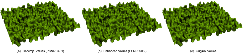
Figure 1. Renderings of an isosurface from Miranda’s Density field: (a) decompressed values by SZ3, (b) enhanced values by NeurLZ, and (c) original values. The enhanced values exhibit noticeable visual improvements over the decompressed ones.

1. Introduction

The exponential growth in computational power has enabled the execution of increasingly complex scientific simulations across a wide range of disciplines. Supercomputers are instrumental in conducting these simulations, allowing users to derive critical insights from vast amounts of generated data. However, despite the enhanced computational capabilities, users often face bottlenecks related to data storage and network bandwidth, particularly when local analysis is required or when large datasets must be distributed across multiple endpoints via data-sharing services. The sheer volume and high velocity of such data present substantial challenges for storage and transmission, underscoring the urgent need for more efficient data compression solutions.

Initially, researchers developed lossless compression algorithms, such as LZ77 (Ziv and Lempel, 1977), GZIP (Peter, 1996), FPZIP (Lindstrom and Isenburg, 2006), Zlib (Gailly and Adler, 2004), and Zstandard (Collet and Kucherawy, 2015), to mitigate data storage and transmission challenges. However, these techniques typically achieve only modest compression ratios (1$\times$-3$\times$) when applied to scientific data (Zhao et al., 2020a). This limitation stems from the fact that lossless compression relies on identifying repeated byte-stream patterns, while scientific data is predominantly composed of highly diverse floating-point numbers. To address this challenge more effectively, researchers have recently turned to error-bounded lossy compression as a promising alternative.

Compared to lossless compressors, lossy compression algorithms (Lindstrom, 2014; Di and Cappello, 2016; Liu et al., 2022, 2023c; Zhao et al., 2021; Tao et al., 2017; Liang et al., 2021, 2019; Tao et al., 2019b; Zhao et al., 2020b; Liang et al., 2018) offer substantially higher compression ratios (e.g., 3.3$\times$ to 436$\times$ for SZ (Di and Cappello, 2016)) while preserving critical information within user-defined error bounds. Many of these lossy compressors rely on predictive techniques, such as curve-fitting (Di and Cappello, 2016) or spline interpolation (Lakshminarasimhan et al., 2013), to estimate the data values. The compression efficiency is closely tied to the local smoothness of the data. However, due to the complexity of scientific simulations, datasets often contain spiky or irregular data points, which pose challenges for predictive compressors. As a result, these compressors frequently need to store the exact values of spiky data points, thereby reducing the overall compression ratio while maintaining a fixed level of error tolerance. To address these challenges, researchers have explored more sophisticated prediction techniques. For example, Zhao et al. introduced higher-order predictors, specifically a second-order predictor (Zhao et al., 2020b), to improve compression performance. Similarly, Tao et al. advanced prediction accuracy for spiky data by employing multidimensional predictors (Tao et al., 2017).

Additionally, implementing a selection mechanism from a pool of predictors has been shown to be advantageous (Di and Cappello, 2016; Tao et al., 2017). Di et al. proposed a method to identify the optimal predictor using just two bits during compression, with the predictor size being negligible, thereby improving the overall compression ratio (Di and Cappello, 2016). Similarly, Tao et al. introduced a suite of multilayer prediction formulas, allowing users to select the most appropriate one based on the dataset characteristics, as different datasets may respond better to specific layers of prediction (Tao et al., 2017). These predictor-based compressors predominantly employ adaptive error-controlled quantization to ensure error levels remain within user-defined bounds. However, despite the high compression ratios achieved by existing lossy compression algorithms, there remains a significant gap between the decompressed data and the original scientific data, particularly when using high error bounds. This discrepancy limits the reconstruction quality, potentially impeding scientific discovery.

Over the past decades, deep neural networks (DNNs) have driven significant breakthroughs across a wide range of foundational and applied tasks in artificial intelligence, including image classification (Rawat and Wang, 2017), object detection (Liu et al., 2020), action recognition (Kong and Fu, 2022), super-resolution (Wang et al., 2020), and natural language processing (Torfi et al., 2020). Researchers have attempted to leverage DNN models, such as those in (Liu et al., 2021, 2023a), to improve compression quality. However, integrating DNNs into lossy compression algorithms presents several key challenges: 1) To effectively retain important information, DNN models are typically large. For instance, the HAT model contains approximately 9 million parameters (Liu et al., 2023a), while the AE model has around 1 million parameters (Liu et al., 2021), leading to significant storage overhead when saving these models to enhance compression. 2) DNN models often require retraining when applied to data from different scientific domains, which can be both time- and resource-intensive. Although pre-trained weights can be provided to eliminate the need for domain-specific retraining, this approach may reduce specificity and compromise performance. 3) DNN models may introduce additional computational costs compared to traditional methods, such as interpolation-based predictors, which typically have linear time complexity.

This paper aims to address the aforementioned challenges and significantly enhance the quality of existing lossy compression techniques. We introduce NeurLZ, a novel cross-field learning-based, error-controlled compression framework. The core innovation of NeurLZ  lies in learning the residual information between the decompressed data produced by lossy compressors and the original data using lightweight skipping DNN models, which integrate cross-field learning with error management. In NeurLZ, decompressed values from each field are processed by the skipping DNN models, which function as learned enhancers. Once trained, the models are appended to the lossy compressors to improve the quality of the decompressed data. Additionally, due to their lightweight design, these DNN models introduce minimal storage and computational overhead, with short training and inference times. Unlike compressors that require extensive pre-training (Liu et al., 2021, 2023a), NeurLZ  offers rapid training of the lightweight models, making it highly adaptable to a wide range of scientific data. In summary, the key contributions of this paper are outlined as follows:

• We propose NeurLZ, a novel cross-field learning-based, error-controlled compression framework, where lightweight skipping DNN models act as enhancers. These models are trained in tandem with the lossy compression process and attached to the compressed data with negligible overhead. To the best of our knowledge, NeurLZ  is the first learn-to-compress, error-controlled framework that addresses the challenges outlined earlier.

• We designed skipping DNN models as enhancers, utilizing a skip connection mechanism to retain high-fidelity details, capture multi-scale information, and recognize complex patterns. This design is particularly suited for scientific data, significantly improving reconstruction quality by preserving essential information.

• By leveraging cross-field relationships derived from the governing equations of scientific simulations, we developed a cross-field learning methodology to enhance our lightweight skipping DNN models. The model incorporates data from multiple fields to predict the target field, capturing cross-field dependencies that traditional lossy compressors typically overlook, thereby improving reconstruction quality.

• Although DNN outputs are often difficult to strictly control, our error management ensures that all values remain within user-defined error bounds. This approach allows us to fully harness the DNNs’ ability to discern complex patterns while effectively mitigating the risks associated with their unpredictability.

• We conducted extensive experiments to evaluate the effectiveness of our approach. The results show significant improvements across multiple datasets, including Nyx, Miranda, and Hurricane. Specifically, experiments on the Nyx Cosmological Simulation Dataset demonstrate a potential relative reduction in bit rate of up to 90%.

2. Background and Motivation

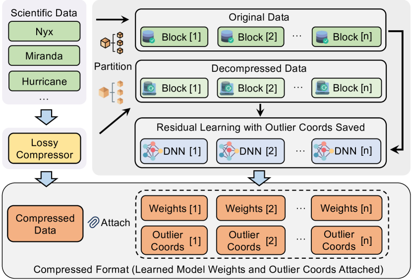
Figure 2. Overview of the NeurLZ compression module (numbers in brackets indicate the corresponding block).

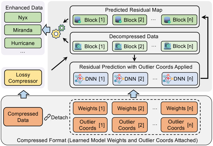
Figure 3. Overview of the NeurLZ reconstruction module (numbers in brackets indicate the corresponding block).

2.1. Lossy Compression

Error-bounded lossy compression offers users the flexibility to select their desired error bound, denoted by $e$. For the given error bound $e$, different lossy compressors may exhibit varying compression quality. Within the lossy compression community, two primary metrics are typically employed to evaluate the compression quality of a lossy compressor: compression ratio and data distortion. Tao et al. pioneered a selection method to optimize between SZ and ZFP compressors (Tao et al., 2019b). Subsequently, Liang et al. further enhanced customization through the modular SZ3 framework (Liang et al., 2022). Data analysis and evaluation were streamlined by Tao et al.’s Z-checker (Tao et al., 2019a). Liu et al. introduced auto-tuning with QoZ, incorporating quality metrics and dynamic dimension freezing (Liu et al., 2022). Their FAZ framework builds upon these advancements, offering a broader range of data transforms and predictors for even greater pipeline customization (Liu et al., 2023b).

Error-bounded lossy compression empowers users to define their desired error tolerance, denoted by $e$. For a specific error bound $e$, different lossy compressors may yield varying levels of compression quality. Within the lossy compression community, two primary metrics are commonly utilized to assess the effectiveness of a lossy compressor: compression ratio and data distortion.

Compression Ratio. The compression ratio $CR$ quantifies the reduction in data size achieved by compression. It is calculated as the ratio of the original data size $|X|$ to the compressed data size $|Z|$, expressed as $CR=|X|/|Z|$. A higher $CR$ indicates more effective compression, meaning the compressed data occupies less storage space.

Data Distortion. Data distortion, inherent to lossy compression, is commonly measured using the Peak Signal-to-Noise Ratio (PSNR). PSNR is a key metric for evaluating the quality of decompressed data from lossy compression. PSNR is defined as follows:

(1) $$\text{PSNR}=20\log_{10}\texttt{vrange}(X)-10\log_{10}\texttt{mse}(X,X^{\prime}).$$

Considering input data $X$ and its corresponding decompressed counterpart $X^{\prime}$, we define vrange as the difference between the maximum and minimum values present within the input data array. Furthermore, let mse represent the mean-squared error quantifying the discrepancy between the original and decompressed data. It is noteworthy that a decrease in mse corresponds to an increase in the PSNR, which serves as an indicator of enhanced fidelity in the decompressed data.

Lossy Compressor and Information Entropy. In 1948, Shannon introduced the concept of information entropy, as defined in Eq. 2 (Shannon, 1948). This definition focuses on a discrete source with a finite number of states, where successive symbols are assumed to be independent. The quantity H(X) is also referred to as the first-order entropy of the source. Due to the lack of prior knowledge about the source, each symbol $X_{i}$ is treated as independently and identically distributed (i.i.d.).

(2) $$H(X)=-\sum_{i}P(X_{i})\log_{2}P(X_{i}),\quad\text{where }X_{i}\text{ are i.i.d.}.$$

First-order entropy typically serves as an upper bound estimate for the true entropy. This is because it is generally larger than higher-order entropy, which accounts for correlations between the $X_{i}$. The consideration of these correlations is equivalent to modeling the source. A common approach for representing such correlations and modeling the source is through the use of Markov models, as illustrated in Eq. 3 (Shannon, 1948).

(3) $$P(x_{n}\mid x_{n-1},\dots,x_{n-k})=P(x_{n}\mid x_{n-1},\dots,x_{n-k},\dots).$$

When a model of the source is sufficiently accurate, the estimated entropy can converge to the true entropy of the source. This provides crucial guidance for data compression, as the entropy defines the minimum average number of bits per symbol needed to encode the data stream. Consequently, Shannon’s theory laid the foundation, and researchers in the field of data compression strive to discover correlations within data to create lower entropy data streams, which can then be efficiently compressed. Lossless compression algorithms such as Huffman Coding (Huffman, 1952), Arithmetic Coding (Rissanen and Langdon, 1979), and LZ77 (Ziv and Lempel, 1977) all exploit correlations between symbols to reduce the estimated entropy, thereby improving the compression ratio.

However, for scientific data, which is typically represented in floating-point format, traditional lossless compression algorithms may not yield satisfactory results. These algorithms are designed to operate on discrete symbols, while floating-point numbers are continuous. Directly applying lossless compression to float data often results in a very low compression ratio. To harness the advantages of lossless compression, float data can be quantized and converted into discrete integer representations. This introduces a degree of lossiness to the compression process, which is often acceptable in scientific applications. Moreover, some lossy compression techniques employ predictors to capture correlations in the data prior to quantization (Chandak et al., 2020; Di and Cappello, 2016; Lindstrom, 2017; Tao et al., 2017; Liang et al., 2022; Zhao et al., 2020b; Liu et al., 2023a; Lakshminarasimhan et al., 2011). These techniques are referred to as prediction-based lossy compressors (Di et al., 2024).

Prediction-based lossy compressors typically involve four steps: pointwise data prediction, quantization, variable-length encoding, and dictionary encoding (Di et al., 2024). The data prediction step aims to identify hidden correlations or patterns within the data, allowing data entries to be predicted from others within a certain tolerance. This prediction is called the first-phase predicted value. In the quantization stage, the error between the first-phase predicted value and the ground truth is mapped to a quantization code. Finally, variable-length encoding and dictionary encoding are used to remove symbol and space redundancy from the quantization codes (Huffman, 1952).

Among these steps, data prediction is arguably the most critical, as higher prediction accuracy can significantly alleviate the burden on subsequent stages (Di et al., 2024). A superior predictor can capture more correlations and effectively encapsulate the underlying knowledge in the data, as demonstrated in Eq. 3 but not limited to this form. This leads to a lower estimation of entropy, which in turn results in a higher compression ratio, since entropy rates are inherently model-dependent. Therefore, constructing a superior predictor that can capture the intricate patterns in scientific datasets remains a formidable challenge in lossy compression.

2.2. Deep Neural Networks

Deep neural networks (DNNs) are a class of artificial neural networks distinguished by their multiple layers of interconnected nodes, or neurons, organized hierarchically. Each layer in a DNN typically performs a nonlinear transformation on its inputs, enabling the network to progressively extract increasingly complex and abstract features from the input data. To train a DNN represented by function $f$, input data $x$ is passed forward through the model, generating predictions $\hat{y}=f(x;\Theta)$, where $\Theta$ represents the network’s parameters. The discrepancy between these predictions and the true values, or ground truth $y$, is then assessed. To optimize the training objective, which is to minimize the loss function (as Eq. 4) with respect to the parameters $\Theta$, the backpropagation algorithm is employed. Backpropagation calculates the gradients of the loss function with respect to the network’s parameters, and these gradients are subsequently utilized to update the parameters through optimization algorithms such as stochastic gradient descent (SGD).

(4) $$\min_{\Theta}~{}\ell(f(\hat{x};\Theta),y),$$

In this research, we adopt an image translation perspective to enhance compression quality. Specifically, we treat the decompressed data as the input image $x$, and the enhanced data as the output image $f(x;\Theta)$. The original, uncompressed data serves as the target $y$ that we aim for the model to produce. The loss function $\ell(\cdot)$ is typically chosen to be the mean square error (MSE), quantifying the difference between the model’s output and the target. Through this process, the DNN is trained to learn the mapping that transforms the decompressed data into a higher-quality representation, effectively enhancing the overall compression quality.

2.3. Skip Connection Structure

Image translation, also known as image-to-image translation, poses a significantly greater challenge compared to traditional tasks like image classification. It demands pixel-level accuracy in the output image. This is particularly critical in scientific or medical domains where images contain crucial information across multiple scales. The task necessitates considering both high-level abstract information and low-level details. Therefore, the ability to capture multi-scale features while preserving low-level details is paramount in image translation tasks.

ResNet’s skip connection architecture (He et al., 2016), empowers it to extract features at various levels, ranging from low to high. These skip connections effectively propagate information from the earlier layers to the deeper ones by directly passing low-level features from the input image to later layers, where they are added to the extracted features. This mechanism aids in retaining the original image’s fine details while allowing deeper layers of the network to focus on extracting high-level features.

The skip connection mechanism is not restricted to the ”add” operation and can also be implemented as a concatenation operation (Ronneberger et al., 2015). In this approach, high-level information channels are concatenated with low-level information channels, and these combined features are then fused to generate the output. Compared to ResNet’s ”add” skip connection, concatenation allows for richer information preservation without merging or losing any details. By having both low-level and high-level features readily available, the network is better equipped to make nuanced decisions during image reconstruction, ultimately leading to more desirable outputs. The inherent advantages of this structure make it particularly well-suited for image translation tasks such as super-resolution (Hu et al., 2019), image denoising (Fan et al., 2022), image generation (Torbunov et al., 2023), and image inpainting (Zhang et al., 2018).

2.4. Problem Formulation

Our research objective in this work is to significantly enhance the compression quality of error-bounded lossy compression. The core problem addressed by our learning-based compression framework can be summarized as follows: How can we substantially improve the fidelity of the reconstructed data (denoted by $X^{\prime}$) from a structured mesh dataset (referred to as $X$) while adhering to a strict user-defined error bound (i.e., $e$) with minimal overhead?

Drawing inspiration from the principles of image translation, where the model learns a mapping from the input image to the output image, our NeurLZ framework leverages this concept to map decompressed data from lossy compressors to the original scientific data. Specifically, we treat the decompressed data as the input image and the original data as the target output image. In this context, the enhanced data generated by the model corresponds to the output of an image translation process. The DNN-based models in our framework are trained to minimize the difference between the decompressed and original data, effectively learning to ”translate” the decompressed data back into its original form. This approach not only improves the quality of the reconstructed data but also ensures that the data adheres to strict error bounds throughout the compression process. Mathematically, the optimization problem can be formally written as:

(5) $$\max_{\Theta} \texttt{PSNR}(X,\mathcal{R}(X^{\prime};\Theta)),$$

s.t. $$|x_{i}-x^{\prime}_{i}|\leq e,\ \forall x_{i}\in X,$$

$$\frac{\texttt{size}(X)}{\texttt{size}(Z)+\textit{overHead}}=T.$$

Here, $X$ represents the input scientific data, $Z$ denotes the compressed data, and $T$ is the target compression ratio. The total storage overhead, denoted as overHead, can be expressed as the sum of two components:

$$\textit{overHead}=\textit{coordsOverhead}+\textit{modelOverhead}$$

where coordsOverhead refers to the storage overhead incurred by storing the coordinates of outlier points (discussed in detail in Section 3.5), and modelOverhead refers to the overhead associated with storing the model parameters. $\Theta$ represents the parameters of the skipping DNN models $\mathcal{R}$ that are trained during the compression process.

The objective is to maximize the PSNR between the original data $X$ and the reconstructed data $\mathcal{R}(X^{\prime};\Theta)$, while ensuring that the error between the original data points $x_{i}$ and their corresponding reconstructed values $x^{\prime}_{i}$ remains within the user-defined error bound $e$, and that the overall compression ratio meets the target $T$. By solving the problem formulated above, our NeurLZ framework can either enhance the PSNR given a specified error bound, or significantly improve the compression ratio while maintaining a fixed PSNR. The following sections will provide a detailed discussion of the specific implementation of NeurLZ.

3. NeurLZ— Learn for Compression

In this section, we present the detailed design of our NeurLZ. The proposed NeurLZ aims to enhance reconstruction quality with minimal overhead by utilizing lightweight learnable enhancers. These enhancers learn the mappings from decompressed data to the original data in a cross-field learning framework with integrated error control mechanisms.

3.1. Design Overview

The NeurLZ framework comprises two primary modules: the compression module and the reconstruction module. These modules are visually represented in Figure 3 and Figure 3, respectively.

In the compression module, a continuous stream of scientific data, exemplified by Nyx, Miranda, and Hurricane, is segmented into blocks of a fixed size, such as (512, 512, 512) for Nyx. Each block is then individually processed by a standard lossy compressor, like SZ3, resulting in compressed data. Conventional lossy compressors require knowledge of whether the decompressed values are within an error bound. Therefore, decompressed data is also generated during the compression process. NeurLZ temporarily stores this decompressed data, and a residual map is calculated between the decompressed data and the original data. The residual map has the same dimensions as both the decompressed and original data. Subsequently, NeurLZ initializes a lightweight DNN model with a skip connection architecture for each block. This model is trained to predict the residual map, essentially representing the compression error, by feeding the decompressed data into the DNN model. Finally, NeurLZ appends the trained weights, W, of these DNN models, which are negligible in size due to their lightweight nature, to the compressed data.

In addition to the trained weights, the coordinates of data points that the DNN model fails to predict accurately are also attached to the compressed data. Since the output of the DNN cannot be fully controlled, some data points may fall outside the error bound even with the predicted residual value, despite the decompressed data generated by the lossy compressor being within the error bound. To address this, we identify and store the coordinates of such data points, referred to as outlier points. This indicates that during decompression, the original decompressed data should be retained for these points, with no residual value added at all. The final compressed format thus comprises the compressed data itself, the trained DNN weights, and the coordinates of these outlier points.

The reconstruction module functions as the counterpart to the compression module. In this module, NeurLZ first extracts the trained weights from the compressed format and uses them to initialize DNN-based enhancer models. Subsequently, NeurLZ decompresses the scientific data block by block. Next, NeurLZ leverages the lightweight DNN models to predict the corresponding residual maps. Finally, the residual map is added to the decompressed data to obtain the initial enhanced data. For data points identified as unpredictable based on the saved coordinates, the corresponding decompressed values replace the enhanced values. This process results in the generation of final enhanced data, which serves as the output of our reconstruction module, as will be introduced in Section 3.5.

3.2. Residual Learning: Improving Training Performance

The primary challenge in the NeurLZ learning process is effectively learning to enhance the decompressed data to closely match the original data. In scientific simulations, the value range can be quite large. For instance, in the Nyx dataset, the Temperature field exhibits a significant range, with the difference between the maximum and minimum values reaching as much as $4.78\times 10^{6}$ (Zhao et al., 2020a). This wide range exacerbates training instabilities due to gradient oscillations, leading to suboptimal training performance.

While it may be challenging to directly predict the original data, it is feasible to estimate the residual data, which is the difference between the original data and the decompressed data. In the field of image restoration, models such as DnCNN (Zhang et al., 2017), MemNet (Tai et al., 2017), and ResDNet (Kokkinos and Lefkimmiatis, 2018) employ residual learning to mitigate training difficulties. Drawing inspiration from this approach, our NeurLZ  also incorporates a residual learning strategy. Specifically, NeurLZ  treats slices of scientific data as single-channel images. Our residual learning approach focuses on learning the residual information ($R=X-X^{\prime}$) between the decompressed data ($X^{\prime}$) and the original data ($X$) on a slice-by-slice basis. By leveraging this design, the magnitude of the learning output is constrained to the level of the error bound, which is significantly smaller than the range of the original data values. Consequently, the model benefits from more stable learning and, once well-trained, can accurately predict the residual information, thereby enhancing the decompressed data to more closely resemble the original data.

The PSNR curves in Figure 5 illustrate the effectiveness of our residual learning strategy over the conventional non-residual approach. We evaluated this across four fields from the Nyx dataset: Dark Matter Density, Baryon Density, Temperature, and Velocity Y. These fields were compressed using the SZ3 lossy compressor with a relative error bound of 1E-3, and then decompressed. In residual learning, we predict the difference between the original and decompressed values (the residual). This approach (orange solid line) consistently boosts PSNR across all fields, indicating a substantial reduction in reconstruction error. In contrast, non-residual learning (green solid line), which directly targets the original values, exhibits less consistent and overall lower performance. These results demonstrate that residual learning provides a robust framework for reducing errors and enhancing the quality of data reconstruction in lossy compression scenarios.

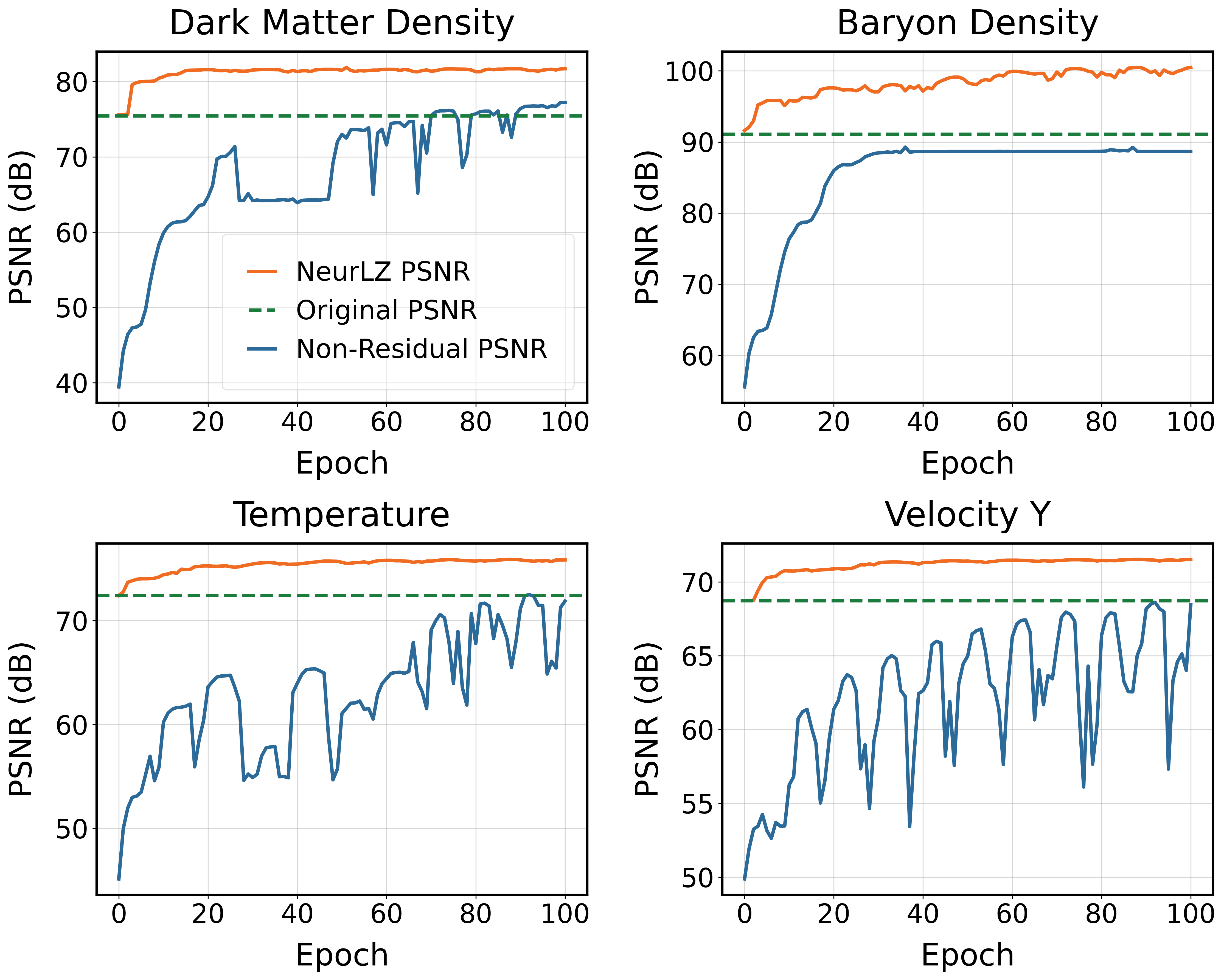
Figure 4. A demonstration of the effectiveness of the NeurLZ  model, which leverages cross-field learning and residual learning within a skipping architecture. In comparison, the non-residual learning model exhibits significantly lower PSNR across all fields in the Nyx dataset. Here, NeurLZ  represents cross-field learning.

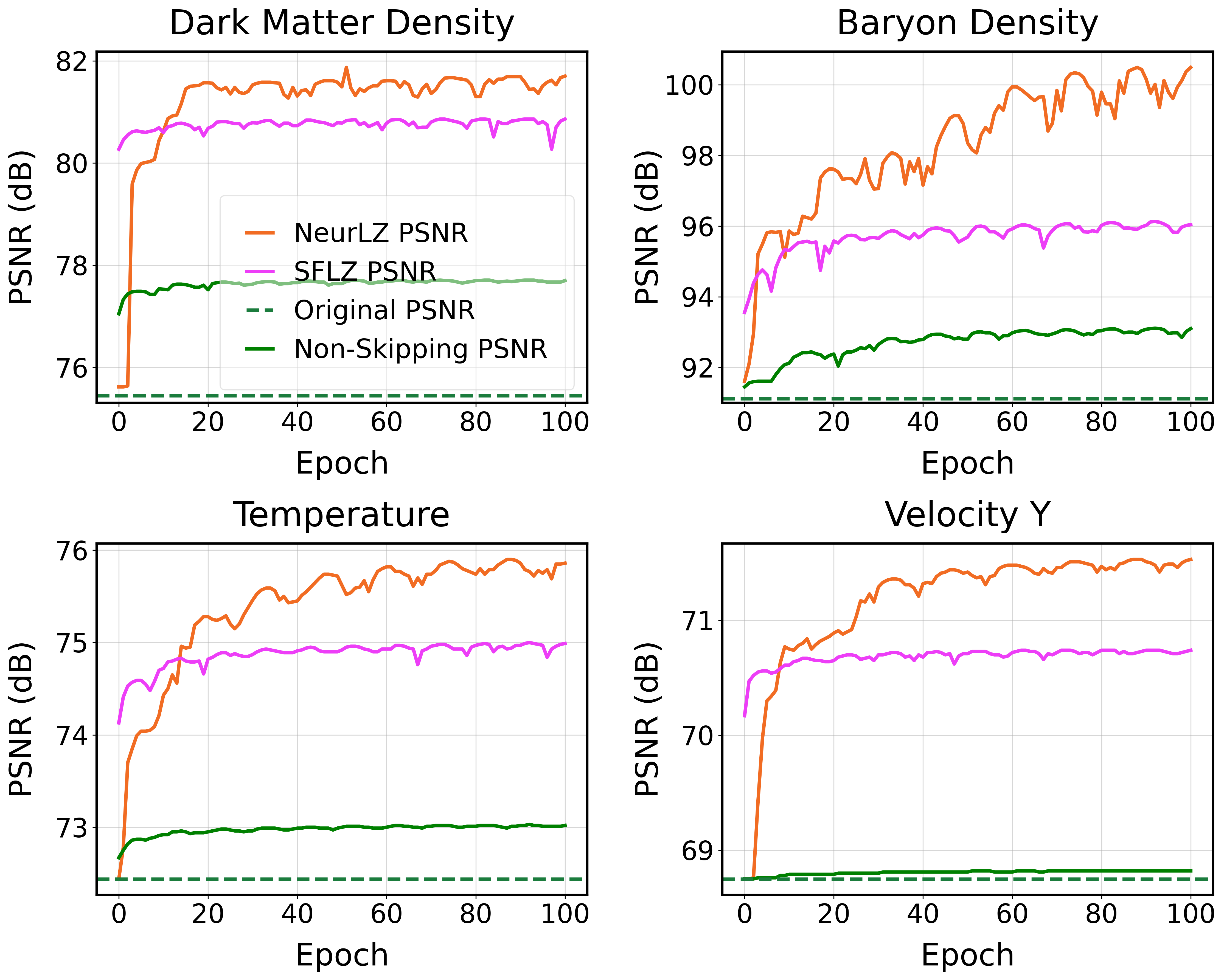
Figure 5. A demonstration of the effectiveness of the NeurLZ  model, which leverages cross-field learning and residual learning within a skipping DNN architecture. Both the non-skipping and single-field learning models show lower PSNR across all fields in the Nyx dataset. SFLZ  denotes single-field learning, while NeurLZ  represents cross-field learning.

Upon completion of the learning process in the NeurLZ compression module, the DNN model predicts the residual map $\hat{R}$ from the decompressed data $X^{\prime}$ generated by the lossy compressor in the NeurLZ reconstruction module. The predicted residual information is then added to the decompressed data, thereby improving the reconstruction quality, i.e., $\hat{X}=X^{\prime}+\hat{R}$.

3.3. Lightweight Skipping DNNs: Representing the Intricate Patterns spanning Scales

As elaborated in Section 2.3, the skip connection structure empowers DNNs to represent intricate patterns spanning various scales. Consequently, we implement this structure and subsequently introduce lightweight skipping DNNs, as illustrated in Figure 6. The input blended slices from decompressed blocks undergoes multiple down-sampling and up-sampling operations via convolution and deconvolution, respectively, to acquire information at different scales. The skip connection then concatenates low-level features with later layers to create a richer representation. Finally, the concatenated features are fused, yielding a single-channel output from the skipping DNN. Furthermore, as discussed in Section 3.2, residual learning is employed to ensure stable learning and achieve optimal training performance (Zhang et al., 2017; Jia et al., 2024). Therefore, the skipping DNN is to predict the residual map with the decompressed slices, which is added to the decompressed slice to produce the enhanced slice via NeurLZ.

Leveraging the advantages of the skip connection structure, specifically its ability to capture multi-scale information, our skipping DNNs can effectively capture complex patterns and preserve high-fidelity details. As demonstrated in Figure 5, the non-skipping model, which lacks these skip connections, exhibits a lower PSNR (green solid line) compared to our NeurLZ  model (orange solid line), which utilizes skip connections. Additionally, the use of convolution and deconvolution operations contributes to the model’s lightweight nature. For instance, a 10-layer network can be constructed with just 3,000 parameters. This compactness makes it particularly well-suited as part of format transmitted to the user, especially when compared to Transformers, which can necessitate billions of parameters (Liu et al., 2023a; Mao et al., 2022).

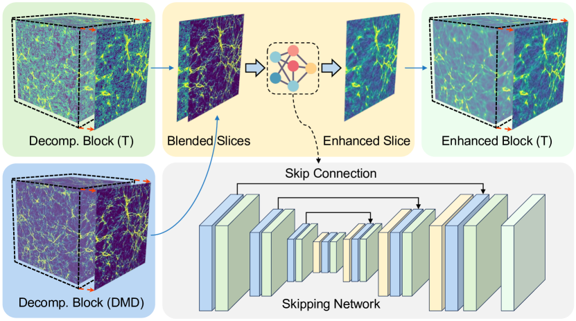
Figure 6. Illustration of NeurLZ learnable enhancer model design based on the skipping architecture. ‘Decomp.’ represents the decompressed data, while ‘T’ and ‘DMD’ represents Temperature and Dark Matter Density fields, respectively, with the former field being enhanced.

3.4. Cross-Field Learning: Capturing the Complex Patterns across Domains

Scientific applications often involve modeling multiple physical fields within a given spatiotemporal domain, such as temperature, velocity, and density in the Nyx cosmological simulation. These simulations are governed by complex equations, such as the Dark Matter Evolution and Self-gravity Equations, which describe the interactions between different fields (Almgren et al., 2013; Lukić et al., 2015; Oñorbe et al., 2019). Existing prediction-based lossy compression techniques (Di and Cappello, 2016; Lindstrom, 2017; Tao et al., 2017; Liang et al., 2022; Zhao et al., 2020b; Liu et al., 2023a) typically rely on predictors that are only capable of capturing localized, simple patterns in time and space. Consequently, these methods fail to exploit the intricate correlations between different physical fields.

In this research, we implement cross-field learning using skipping DNNs to capture the complex patterns that span across different domains. An illustration of cross-field learning is shown in Figure 7. To predict the value of a single pixel (indicated by the red cube in the Temperature field), our approach utilizes not only the values of neighboring pixels but also the values from pixels in two other fields. Moreover, the patterns of values utilized are not fixed but are instead learnable. The skipping models are trained to identify these patterns across different fields. Consequently, once the model is trained, the prediction for a single pixel is informed by data from both the same field and from different fields. By learning these cross-domain correlations, the skipping model provides a more accurate representation of the underlying information source that generates the scientific data. This leads to a lower entropy estimation, consequently yielding a higher compression ratio, as discussed in Section 2.1.

Delving into the implementation specifics, Figure 6 illustrates how a skipping model is trained to capture patterns across two distinct fields - Temperature (T) and Dark Matter Density (DMD) - with the goal of predicting the target field, Temperature. Decompressed slices from both two fields serve as the 2-channel input, and the model predicts the residual map for Temperature after fusing multiple channels before the final layer. The residual map is then added to the decompressed slice to produce an enhanced slice via NeurLZ. Figure 5 illustrates the advantages of cross-field learning over traditional single-field learning. Although single-field learning (purple solid line) offers some improvement over the original PSNR (green dashed line), it consistently underperforms compared to cross-field learning (orange solid line) across all fields in the Nyx dataset. This highlights the enhanced capability of cross-field learning in capturing complex dependencies and improving model performance.

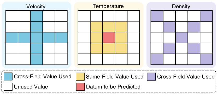
Figure 7. An illustration of cross-field learning: The prediction of a datum is contributed not only by neighboring values in the same field but also by values from other fields in learnable patterns.

3.5. Outlier Points Management: Providing the Strict Error Bounds

As outlined in Section 3.1, the inherent uncontrollability of DNN output means that some data points, even when enhanced with predicted residual values, might exceed the error bound, even if the lossy compressor’s decompressed data remain within it. We refer to these points as outlier points. To uphold the error-bounded guarantee, we implement a strategy that draws inspiration from SZ3’s approach of differentiating between predictable and unpredictable values using distinct quantization codes. Just as SZ3 retrieves the original value from an unpredictable queue upon encountering a 0 quantization code during decompression (Tao et al., 2017), we similarly store the coordinates of outlier points - those data points whose enhanced values, derived from the addition of predicted residual values, lie beyond the acceptable error threshold as depicted on the left side of Figure 8. Subsequently, once the enhanced values are computed, we leverage these stored coordinates to pinpoint and address these outliers. We replace their out-of-bound enhanced values with their corresponding in-bound decompressed values, ensuring that all data points remain within the predefined error limits, as illustrated on the right side of Figure 8. This approach, mirroring SZ3’s mechanism of handling unpredictable values, empowers us to effectively manage and rectify outliers. By adopting this strategy, we can fully leverage the capabilities of DNNs in discerning complex patterns while simultaneously mitigating the inherent risks associated with their uncontrollability. This guarantees that the enhanced data consistently adheres to the specified error bound, thereby preserving the accuracy and reliability of the data representation.

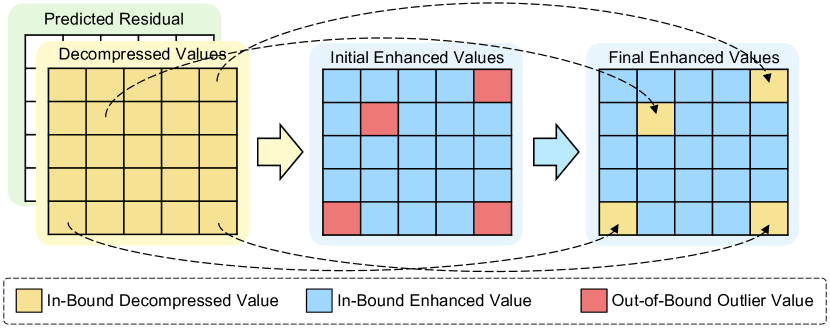
Figure 8. An illustration of outlier management: First, decompressed values are enhanced by adding predicted residuals, resulting in initial enhanced values, some of which may be out-of-bound outlier values. These outliers are then replaced with in-bound decompressed values to produce the final enhanced values, ensuring all values adhere to the error bound.

Storage Overhead for Outlier Coordinates. As discussed earlier, NeurLZ  provides a strict error bound by storing the integer coordinates of outlier points to index the decompressed data and retrieve the corresponding decompressed values. The storage overhead for these coordinates is calculated as follows:

(6) avgBit $$={\sum_{i=1}^{N}\log_{2}(\textit{dim}_{i})}$$

coordsOverhead $$=\textit{numOutliers}\times\textit{avgBit}$$

Here, dim_i represents the size of the $i$-th dimension, while avgBit denotes the average number of bits required to store the N-dimensional coordinates of a single datum. numOutliers refers to the number of outlier points. coordsOverhead is the storage overhead incurred by storing the coordinates of outlier points, expressed in bits, calculated by multiplying avgBit by numOutliers. For the scientific datasets discussed in this paper, the block size for Nyx is $(512,512,512)$ with an avgBit of 27.0 bits; for Miranda, the block size is $(256,384,384)$ with an avgBit of 25.2 bits; and for Hurricane, the block size is $(100,500,500)$ with an avgBit of 24.6 bits. These values highlight the variability in storage overhead depending on the dataset’s dimensionality and structure.

Regulated Neural Network Output. In some cases, the overhead for storing the coordinates of outliers may be excessively large, as will be shown in Section 4.2. For users concerned about size, we apply DNN output regulation to provide a 2$\times$ error bound for each datum without the need to save the coordinates of outliers. As illustrated in Figure 9, consider one datum as an example: the original value (red star) of that datum is compressed and decompressed within a 1$\times$ error bound by lossy compressors, with the possible decompressed value distribution shown as the red band. The worst-case decompressed value would be the near-bound decompressed value (yellow star), which is exactly 1$\times$ error bound away from the original value. In this scenario, the near-bound decompressed value is forwarded into the DNN to obtain the enhanced value for the datum, with the possible enhanced value distribution represented by the blue band. Although we cannot precisely control the neural network’s output, we can regulate its output within a certain range.

Figure 9 illustrates three cases, each with a DNN that has a different degree of output regulation. In Case A, the DNN is tightly regulated, ensuring that its minimal possible enhanced value does not exceed the 2$\times$ error bound. However, its maximum possible enhanced value does not reach the original value, which may limit the DNN’s performance. In Case B, the DNN is balanced in its regulation, where the minimal value exactly meets the 2$\times$ error bound, and the maximum value exactly reaches the original value, allowing the DNN to potentially enhance the decompressed value to the original value through learning. In Case C, the DNN has loose regulation: while its maximum value exceeds the original value, meaning it could hit the original value, the minimal value also exceeds the 2$\times$ error bound. This may result in the DNN ’enhancing’ the decompressed value to a level outside the 2$\times$ error bound, potentially reducing reconstruction performance.

In NeurLZ, to achieve balanced regulation, we normalize the residual values using the error bound and append one Sigmoid layer to the skipping DNN to regulate the output within the range [0, 1]. This approach ensures balanced regulation and guarantees the 2$\times$ error bound. By default, to ensure a strict error bound, NeurLZ  saves the coordinates of the outlier points. All the results presented in this paper are based on this approach. However, if users choose not to save the coordinates of these outlier points, the compression ratio will be significantly improved, as shown in Section 4.2. We also found that these outlier points, which exceed the 1$\times$ error bound but remain within the 2$\times$ error bound, do not significantly impact the PSNR, as demonstrated in the results presented in Section 4.2.

Figure 10 presents the evolution of PSNR and maximum absolute error during training for two fields in the Nyx dataset: Dark Matter Density and Temperature, under two scenarios: the regulated NeurLZ  and the unregulated case. Both cases enhanced the SZ3 compressor with a 1E-3 error bound. While both cases ultimately achieved similar PSNR levels, the regulated NeurLZ  exhibited a more stable training process. Additionally, the regulated NeurLZ’s maximum error was consistently maintained within the 2$\times$ error bound, whereas the unregulated case exceeded this limit. The Sigmoid layer’s regularization mechanism introduced prior knowledge into the model, facilitating smoother training and ensuring adherence to the 2$\times$ error bound.

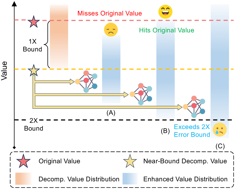
Figure 9. An illustration of how neural network regulation affects the error bound of enhanced values. The decompressed value distribution from a lossy compressor is shown as the red band, with the worst-case near-bound value (yellow star) passed through three neural networks: tight regulation (Case A), balanced regulation (Case B), and loose regulation (Case C). The resulting enhanced value distributions (blue bands) show that in Case A, the maximum enhanced value misses the original value; in Case B, it hits the original value; and in Case C, while it hits, the minimum enhanced value exceeds the 2$\times$ error bound.

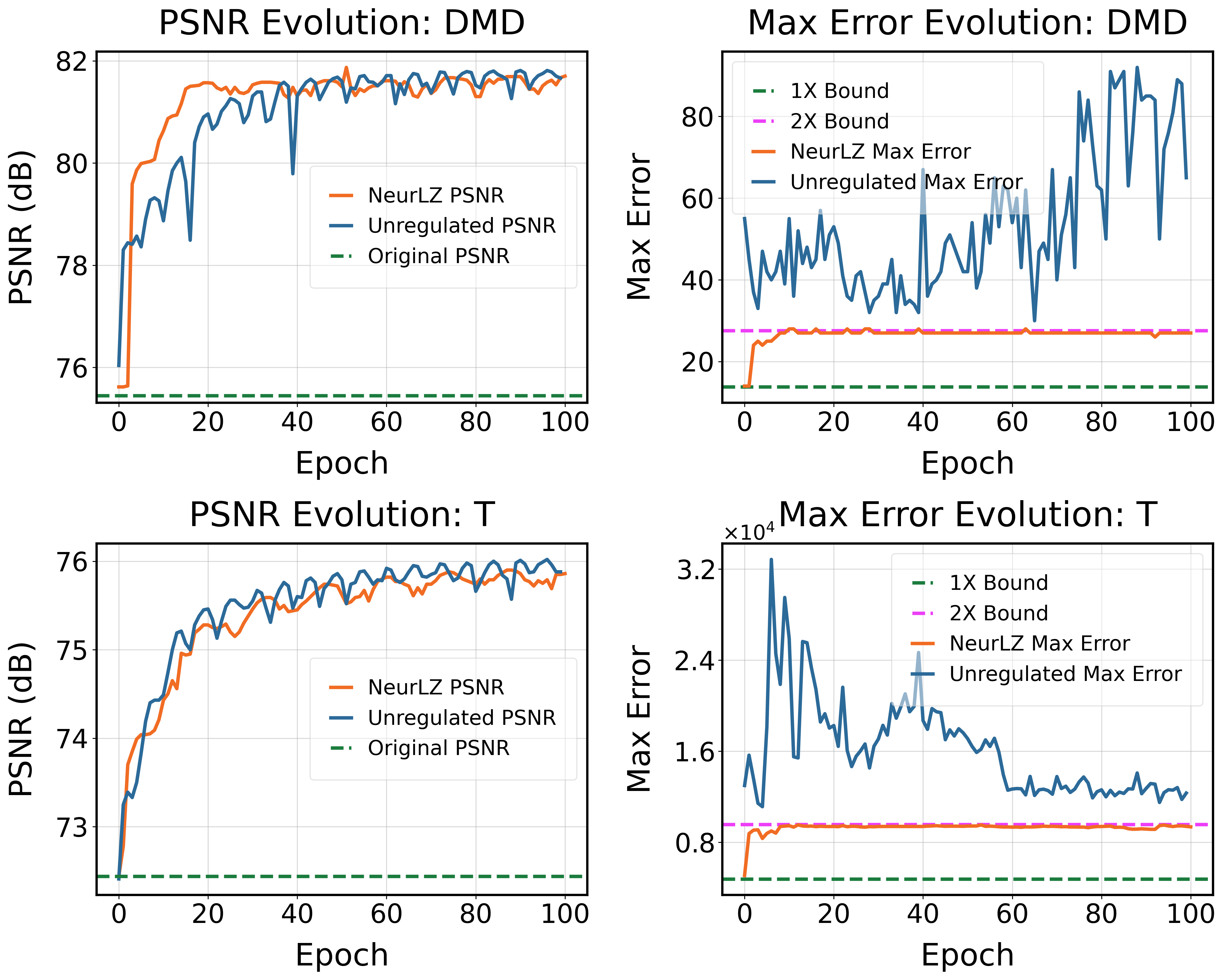
Figure 10. Evolution of PSNR and max absolute error during training for the Dark Matter Density (DMD) and Temperature (T) fields in the Nyx dataset, comparing NeurLZ  (regulated) with the unregulated case. Both cases enhance the SZ3 compressor with a 1E-3 error bound. The unregulated case shows higher max absolute errors over 2$\times$ the bound, while NeurLZ  maintains stable performance within 2$\times$ the bound.

4. Evaluation

This section outlines the experimental design used to assess the performance of NeurLZ, a novel cross-field learning-based, error-controlled compression framework for scientific data. We will subsequently describe the experimental setup and present the results, followed by a comprehensive analysis.

4.1. Experimental Setup

Experimental Environment. Our experiments are conducted on two servers, each equipped with eight NVIDIA RTX 6000 Ada GPUs, two AMD EPYC Genoa 9254 CPUs (each with 24 cores), and 1.5 TB of DRAM.

Datasets. Table 1 lists the three datasets used in our experiments: Nyx, Miranda, and Hurricane. The Nyx dataset, generated by the adaptive mesh, compressible cosmological hydrodynamics simulation code Nyx (Almgren et al., 2013), is a popular choice in the cosmological research community. It contains six 3D array fields, each with a shape of 512 $\times$ 512 $\times$ 512. Figure 13 showcases two of these fields: Temperature and Dark Matter Density. The Nyx dataset is stored in FP32 format. The Miranda dataset, produced by a structured Navier-Stokes flow solver with multi-physics capabilities, is designed for large turbulence simulations (Cook and Cabot, 2024). It consists of seven 64-bit double-precision floating-point fields, each with dimensions of 256 $\times$ 384 $\times$ 384. The Hurricane ISABEL dataset, derived from a simulation of the 2003 Atlantic hurricane season’s most intense hurricane, includes 13 single-precision floating-point fields, each a 3D array of size 100 $\times$ 500 $\times$ 500. To assess the performance of NeurLZ, we employed sample blocks of these datasets provided by SDRBench (Zhao et al., 2020a).

Table 1. Information of the datasets in experiments (Zhao et al., 2020a).

Dataset	Domain	Dimensions	Per Block Size	Data Type
Nyx	Cosmologicial	3D	(512, 512, 512)	FP32
Miranda	Large Turbulence	3D	(256, 384, 384)	FP64
Hurricane	Weather	3D	(100, 500, 500)	FP32

Learning Configurations. As illustrated in Figure 6, NeurLZ  incorporates skipping DNN models as enhancers. Each model employs four down-sampling and up-sampling operations with skip connections, totaling approximately 3,000 parameters. The training process utilized 8 GPUs with a batch size of 10 over 100 epochs. The initial learning rate was set to 1E-2, and a cosine annealing learning rate schedule was implemented. Upon training completion, all DNN model weights were integrated into the final compressed data format, using either FP32 or FP64 precision based on the dataset’s precision.

Compressor. NeurLZ  is a flexible framework that can accommodate various lossy compressors, as depicted in Figure 3 and Figure 3. This paper focuses on two representative examples: the prediction-based error-bounded SZ3 (Liang et al., 2022) and the transform-based error-bounded ZFP (Lindstrom, 2014). As outlined in Section 2.1, data prediction plays a crucial role in prediction-based lossy compressors such as SZ3, as a superior predictor can effectively capture correlations and reduce entropy estimation. NeurLZ  acts as an enhancer, capturing correlations that SZ3 might overlook, thereby further reducing entropy estimation and improving compression ratio. While ZFP does not explicitly predict data, it utilizes orthogonal transforms to decorrelate the data (Di et al., 2024), achieving a similar goal of eliminating redundancy and reducing entropy estimation. Therefore, ZFP was chosen to assess the performance of NeurLZ  with transform-based lossy compressors.

Performance Evaluation Criteria. NeurLZ  enhances decompressed values using error bounds provided by lossy compressors. In SZ3, we use a value-range-based relative error bound (denoted as $e$), which corresponds to the absolute error bound $\epsilon$ in ZFP. The relationship between them is given by $e=\epsilon\cdot value\_range$, where $value\_range$ represents the data block’s value range being compressed. For simplicity, throughout this paper, we refer to the error bound uniformly as $e$. When dealing with ZFP, $\epsilon$ is converted to the corresponding $e$. Each experiment is characterized by the compressor type, the error bound, the dataset, and the specific field. We evaluate NeurLZ  with the criteria described below:

• Decompression error validation: Verifying that NeurLZ’s error is strictly bounded by the user-defined error threshold.

• Enhanced data visualization: Evaluating the visual quality of the enhanced data compared to the original decompressed data.

• Bit rate vs. PSNR curves: Displaying PSNR values at various bit rates for different compressors. A lower bit rate for the same PSNR or a higher PSNR at the same bit rate is preferred.

• The relative reduction (%) in bit rate at equal PSNR: Comparing the reduction in bit rate between NeurLZ  and corresponding compressors, such as SZ3 and ZFP, while maintaining the same PSNR.

4.2. Experimental Results

Decompression Error Validation. Since the decompression error originates from the training process, we first examine the training dynamics. Figure 12 presents two experiments on the Nyx dataset’s Dark Matter Density and Temperature fields, where NeurLZ  enhances the SZ3 compressor with a relative error bound of 1E-3. The results show that the PSNR of NeurLZ  increases rapidly and significantly exceeds the original PSNR. Around 100 epochs, the PSNR improvement stabilizes. The figures also display the Outlier Rate (OLR) (%), which indicates the percentage of outlier points relative to the total data points. A lower OLR results in reduced overhead, referred to as coordsOverhead, for storing the coordinates of outlier points, as discussed in Section 3.5. As the PSNR improves, the OLR rapidly decreases to 0.01%, leading to a further reduction in overhead. Consequently, the significant PSNR improvement and reduced coordsOverhead result in bit rate reductions of approximately 66.4% and 36.3%, as shown in Table 2.

After training, the coordinates of outliers—those exceeding 2$\times$ the error bound—are saved and attached to the compressed format. During decompression, based on the stored coordinates, the values of the outlier points are first enhanced and then replaced with in-bound decompressed values, resulting in the final enhanced values, as discussed in Section 3.5. This process ensures the strict error bound is respected. In Figure 12, different experiments on the SZ3 compressor are shown with a stricter error bound of 5E-5. NeurLZ  ensures that no points exceed this 5E-5 error bound, demonstrating that all errors are confined within the specified limit. Compared to the original error distribution by SZ3, NeurLZ  exhibits a more concentrated distribution, indicating reduced entropy.

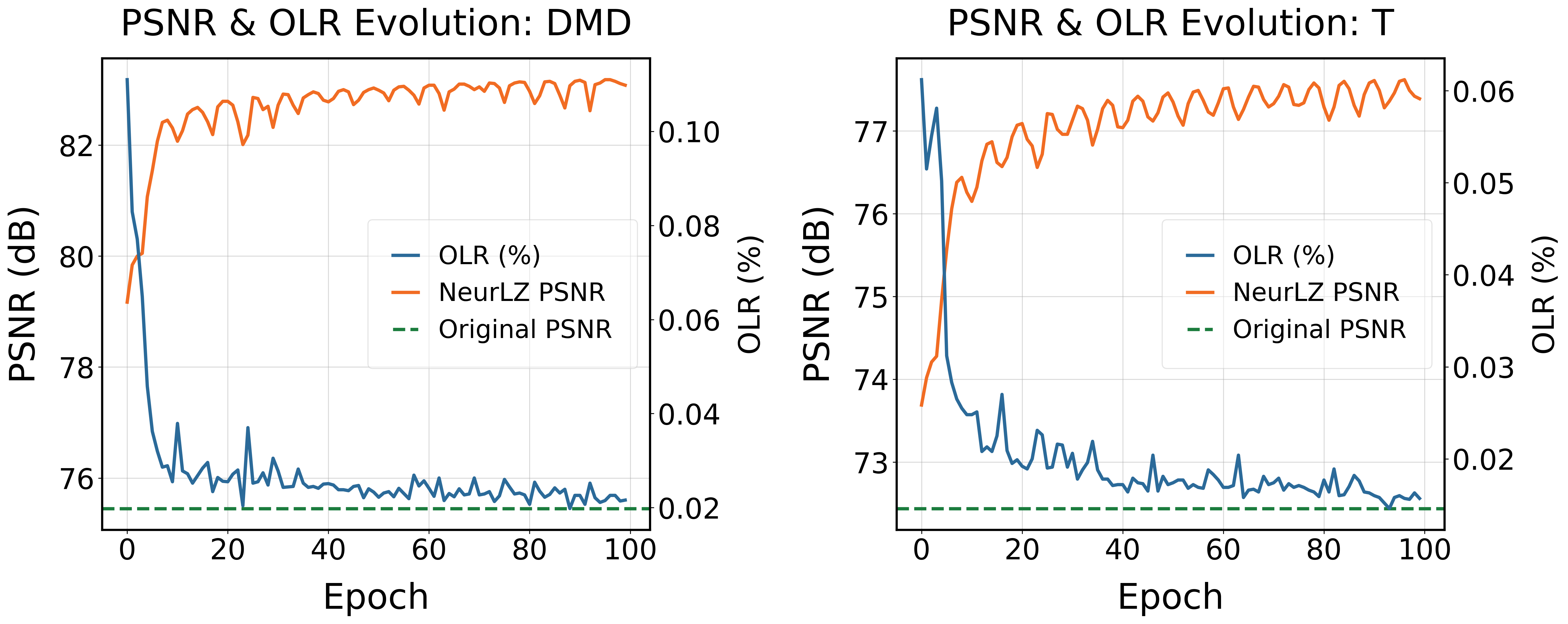
Figure 11. An illustration of the evolution of PSNR and outlier rate (OLR) (%) during training for the Dark Matter Density (DMD) and Temperature (T) fields in the Nyx dataset. The PSNR was obtained using NeurLZ, which enhances the SZ3 compressor with a relative error bound of 1E-3.

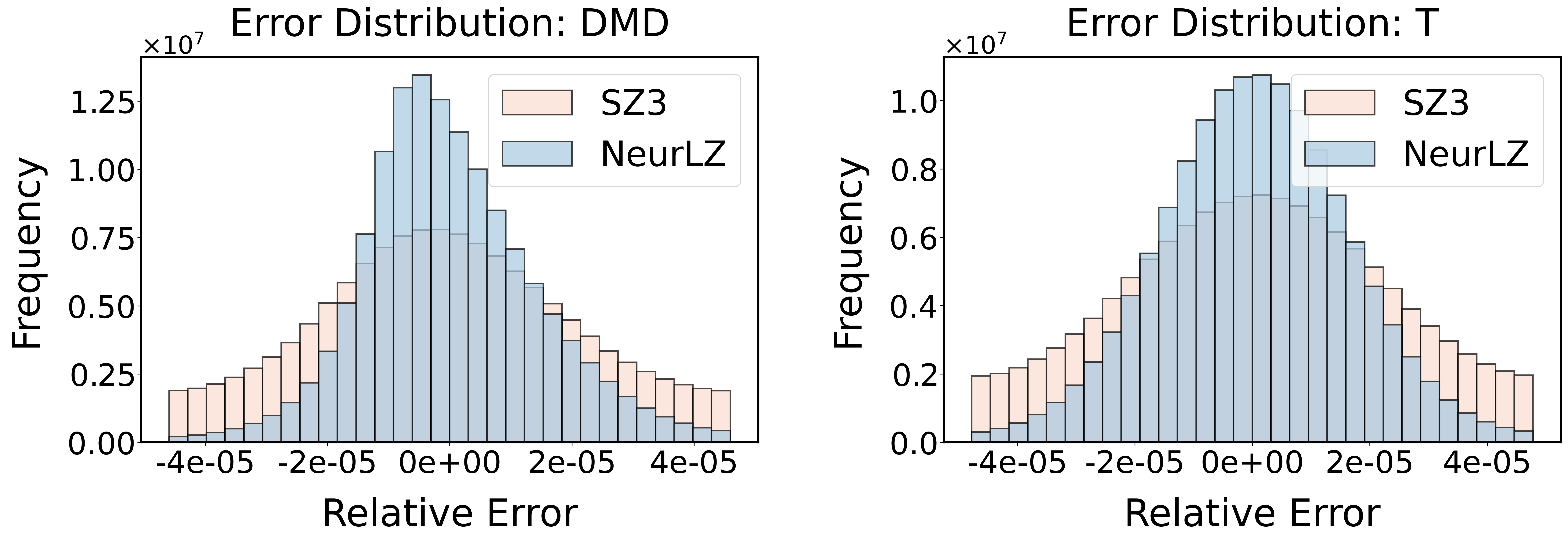
Figure 12. Error distribution for the Dark Matter Density (DMD) and Temperature (T) fields, generated between SZ3 decompressed values and NeurLZ-enhanced values against the original values, under a relative error bound of 5E-5.

Enhanced Data Visualization. Figure 13 visually compares the original, decompressed, initial enhanced, and final enhanced values of the Temperature and Dark Matter Density fields from the 128^th slice along the first dimension of the Nyx dataset. All values have a shape of (512, 512). To facilitate visualization given the wide value range, a log scale was employed. The decompressed values were obtained using the SZ3 compressor with a relative error bound of 5E-5, while the initial and final enhanced values were generated by NeurLZ. The results clearly demonstrate that both the initial and final enhanced values exhibit superior visual quality compared to the decompressed values, further supported by the PSNR improvements.

For the Temperature field, the decompressed image has a PSNR of 92.7, whereas the final enhanced version achieves a PSNR of 95.7. From a visual perspective, NeurLZ  provides a more detailed reconstruction than SZ3. In the Dark Matter Density field, the decompressed values from SZ3 exhibit noticeable noise, particularly in the background regions with lower dark matter concentrations, resulting in a PSNR of 92.9. In contrast, the enhanced values from NeurLZ  significantly reduce the noise, yielding a background that closely resembles the original values, as reflected in an improved PSNR of 96.3. This demonstrates that the skipping DNN models effectively mitigate noise, leading to a notable increase in PSNR.

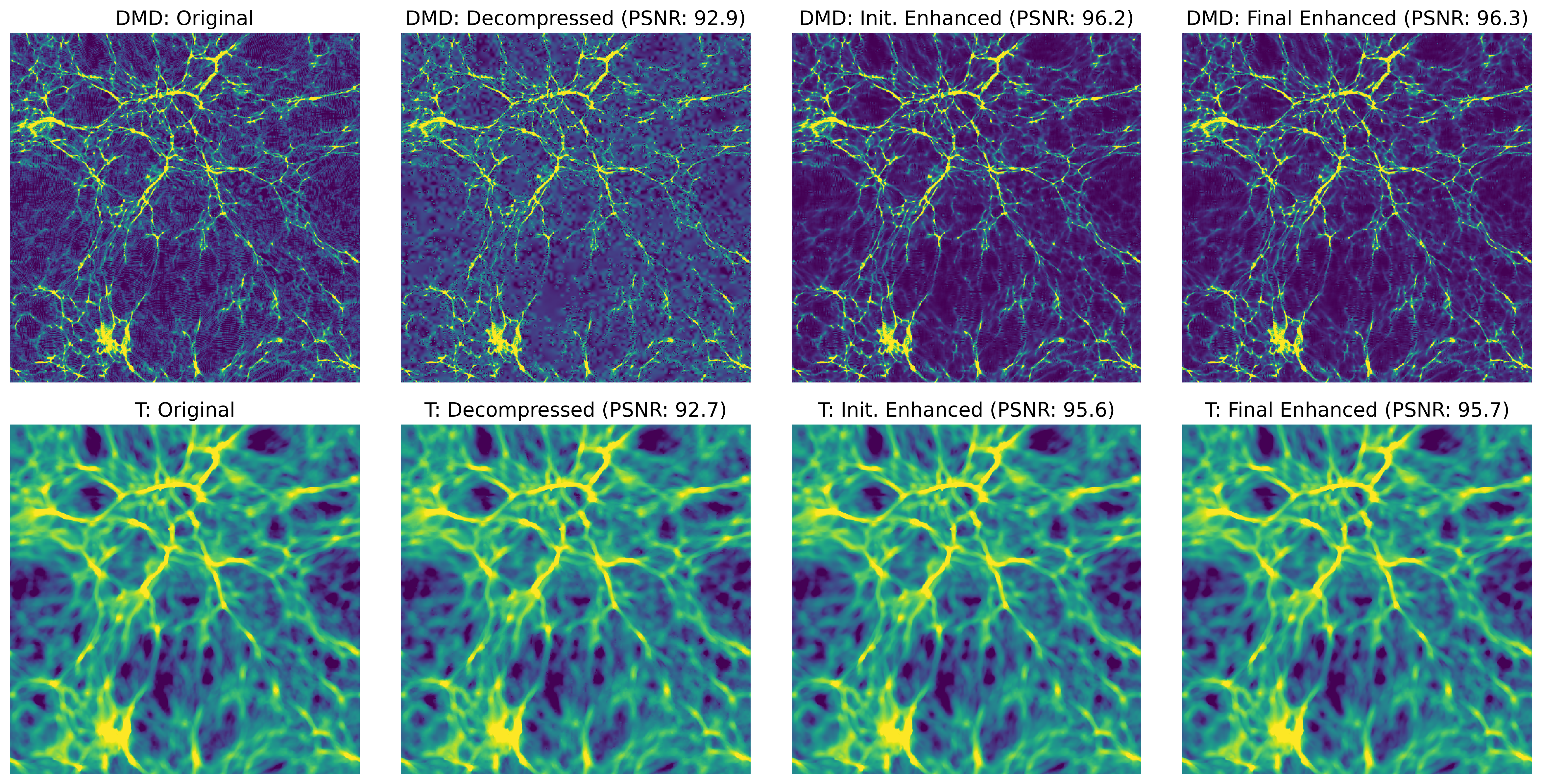
Figure 13. A comparison of original, decompressed, initial enhanced, and final enhanced values for Dark Matter Density (DMD) and Temperature (T) fields from a single slice of the Nyx dataset. The decompressed values are obtained using the SZ3 algorithm with a relative error bound of 5E-5, while the enhancement is achieved using NeurLZ.

Bit rate vs. PSNR Curves. The bit rate reflects the average number of bits required to represent one datum. It is calculated as follows:

$$\textit{bitRate}=\frac{\texttt{size}(Z)+\textit{overHead}}{\textit{numPoints}}$$

where $\texttt{size}(Z)$ denotes the size of the compressed data $Z$, typically measured in bits. The overHead represents the total storage overhead, which includes the storage of the coordinates of outlier points and the storage associated with model parameters, as discussed in Section 2.4. The numPoints is the total number of data points in the original uncompressed dataset. Therefore, the bit rate not only reflects the size of the compressed data but also takes into account the outliers and model parameters, making it a more comprehensive measure of the average storage cost.

Figure 15 presents the Bit rate vs. PSNR curves for SZ3, SFLZ, and NeurLZ  to compare their performance across different fields in the Nyx dataset. Each point on the curves corresponds to an experiment conducted with a specific error bound for the associated field. Multiple error bounds were selected to offer a comprehensive evaluation of performance. Single-field learning (SFLZ) and cross-field learning (NeurLZ) were applied to enhance SZ3’s decompressed values, providing a comparative analysis of their effectiveness. In these Bit rate vs. PSNR curves, a curve that entirely encloses another within the upper-left region of the graph indicates superior performance. This suggests that the method achieves higher PSNR at the same bit rate or maintains the same PSNR with a lower bit rate, demonstrating better compression efficiency. Our results clearly demonstrate that for each field, NeurLZ’s curve consistently encloses SFLZ’s curve, and SFLZ’s curve consistently encloses SZ3’s curve. This indicates that NeurLZ  consistently outperforms SFLZ, and SFLZ  outperforms SZ3.

Beyond the simple containment relationship, the area between the curves over the specified interval provides additional insights. The area between SFLZ’s and SZ3’s curves reveals the impact of contribution derived from the single-field relationships captured by SFLZ. We observed that Temperature, Velocity X, Velocity Y, and Baryon Density exhibit similar levels of area between NeurLZ’s and SZ3’s curves across different intervals. This suggests that skipping DNN models effectively captures correlations that SZ3 fails to capture, even within the same field, leading to superior performance. For Dark Matter Density, increasing the bit rate results in a smaller area, suggesting a diminishing performance advantage for NeurLZ. Conversely, for Velocity Y, even with a higher bit rate (which might be challenging due to the low compression ratio), the area increases, indicating that skipping DNN models is particularly effective in capturing patterns in this scenario.

The area between NeurLZ’s and SFLZ’s curves provides insight into the extent of contribution derived from cross-field relationships captured by NeurLZ. While NeurLZ’s curve consistently encloses SFLZ’s across all fields, the variation in the area across different intervals and fields suggests differing levels of attribution from cross-field learning. In the Temperature, Dark Matter Density, Velocity X, and Velocity Y fields, the area initially decreases, then increases, and finally decreases again, indicating that the contribution from cross-field learning varies, first starting small, then growing, and eventually diminishing. In contrast, Velocity Z consistently shows a smaller area, suggesting that either fewer cross-field relationships are captured by NeurLZ, or that such relationships are inherently limited. For Baryon Density, the area remains large throughout, with no reduction as the bit rate increases. This indicates that the majority of cross-field relationships are effectively captured, resulting in the most significant improvements.

Beyond the improvements observed with the SZ3 compressor, the impact of NeurLZ  on the ZFP compressor was also examined. Figure 15 displays the Bit rate vs. PSNR curves for ZFP, SFLZ, and NeurLZ, illustrating their relative performance across the Nyx dataset fields. Similar to our previous analysis, both single-field learning (SFLZ) and cross-field learning (NeurLZ) were integrated with ZFP to enhance its decompressed outputs. The results reveal that NeurLZ  consistently surpasses SFLZ, and both outperform the baseline ZFP, as shown by the progressive curve enclosures.

Regarding the area between SFLZ’s and ZFP’s curves, we observed that for Temperature, Dark Matter Density, and Baryon Density, the area remains constant as the bit rate increases, suggesting that SFLZ  primarily captures single-field relationships. For the three velocity fields (Velocity X, Velocity Y, and Velocity Z), the area approaches zero with increasing bit rate, indicating minimal improvement from SFLZ. While SFLZ’s improvements for these three fields are limited, NeurLZ’s performance gains are significant. When cross-field learning is employed, the area between NeurLZ’s and SFLZ’s curves exceeds that between SFLZ’s and ZFP’s curves, highlighting the greater impact of cross-field learning in the ZFP setting compared to the SZ3 setting, where SFLZ  already demonstrates significant improvement. Among Temperature, Dark Matter Density, and Baryon Density, the latter exhibits the largest area between NeurLZ’s and SFLZ’s curves, indicating the most significant benefits of cross-field learning. Although these improvements are not as substantial as those achieved with the SZ3 compressor (as detailed in Table 2), this is understandable given that ZFP is a transform-based compressor, while SZ3 is a prediction-based compressor. Nevertheless, NeurLZ’s improvements on the ZFP compressor demonstrate its ability to capture relationships that ZFP’s transform module overlooks, particularly across fields.

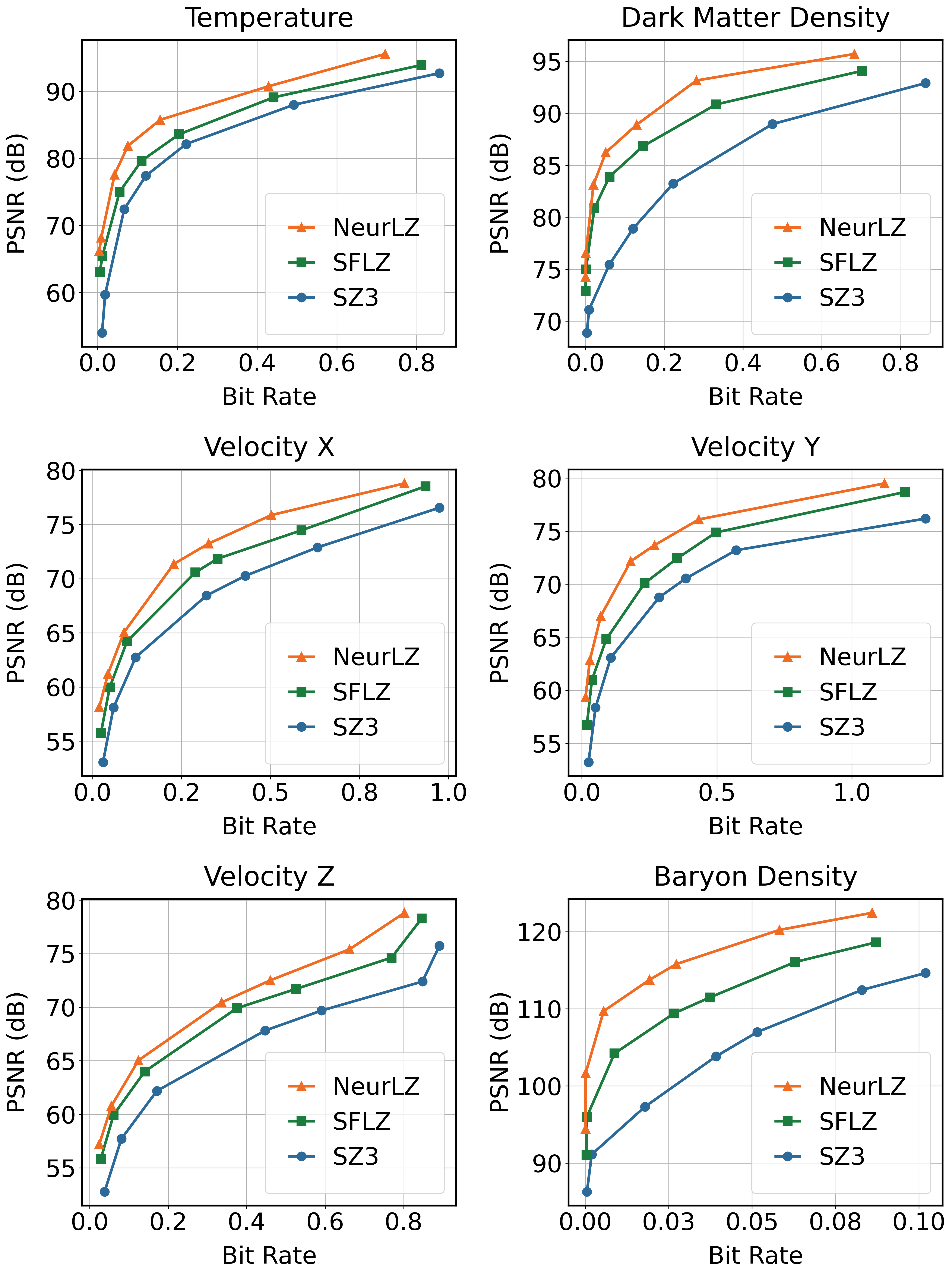
Figure 14. Bit rate comparison for the Nyx dataset using three different methods: SZ3, SFLZ, and NeurLZ. Here, SZ3 refers to the original SZ3 compression algorithm, SFLZ  stands for single-field learning with SZ3, and NeurLZ  represents cross-field learning with SZ3.

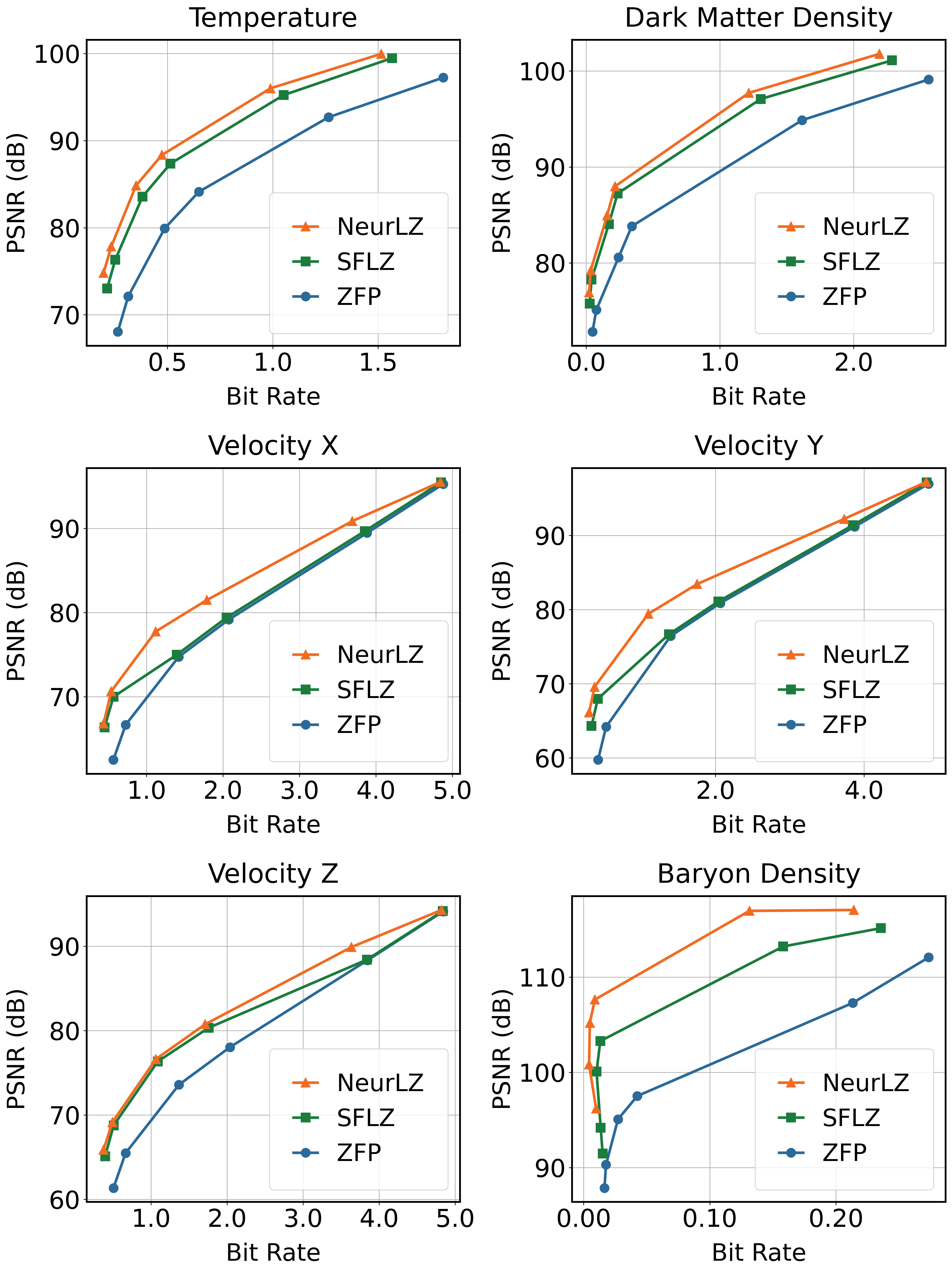
Figure 15. Bit rate comparison for the Nyx dataset using three different methods: ZFP, SFLZ, and NeurLZ. Here, ZFP refers to the original ZFP compression algorithm, SFLZ  stands for single-field learning with ZFP, and NeurLZ  represents cross-field learning with ZFP.

The Relative Reduction (%) in Bit Rate at Equal PSNR. To quantitatively assess the improvements achieved by NeurLZ, three datasets introduced in Section 4.1 were tested using different relative error bounds on the SZ3 and ZFP compressors. For SZ3, relative error bounds ranging from 1E-2 to 1E-4 were applied, while for ZFP, bounds from 1E-1 to 1E-3 were used. The rationale for applying different error bounds to SZ3 and ZFP is to maintain comparable PSNR ranges. ZFP’s error distribution is more conservative, resulting in higher PSNR values under the same error bound (Tao et al., 2017), thus a more relaxed error bound was chosen for ZFP. Table 2 presents the relative reduction (%) in bit rate at equal PSNR for each experiment. This metric indicates the extent to which NeurLZ  has reduced bit rate compared to SZ3 or ZFP while maintaining the same PSNR. For instance, in the Nyx dataset’s Temperature field at the error bound of 1E-2, NeurLZ  achieved a 62.9% and 28.0% bit rate reduction compared to SZ3 and ZFP, respectively.

NeurLZ  has achieved significant overall improvements on the SZ3 compressor. Notably, for the Nyx dataset’s Dark Matter Density field with an error bound of 1E-2, the relative reduction in bit rate reaches as high as 89.1%. Among the Nyx fields, Dark Matter Density and Baryon Density both show reductions exceeding 40.0% across all error bounds. The Temperature field also exhibits a substantial reduction, particularly 62.9% at the 1E-2 error bound. For all fields, except Baryon Density, the reduction decreases as the error bound becomes stricter. Specifically, for the three velocity fields, the reductions fall below 5.0% at the 1E-4 error bound, which will be further analyzed in Section 5. Interestingly, the Baryon Density field demonstrates a 69.0% reduction at the 1E-4 error bound, higher than the 50.1% reduction at 1E-2. This may indicate that NeurLZ  captures more relationships missed by SZ3 under the 1E-4 error bound compared to the 1E-2 error bound, even with the stricter conditions of the former.

For the Miranda dataset, although no fields are enhanced as significantly as Dark Matter Density and Baryon Density in the Nyx dataset, the overall performance remains strong. Most fields, except for Density, show approximately a 20% reduction even at the strict error bound of 1E-4. A similar pattern observed in Nyx, where stricter error bounds result in decreased reductions, is also evident in Miranda. Across all fields, the highest reductions are achieved at looser error bounds, while the smallest reductions occur at stricter error bounds.

In contrast, the performance enhancement for the Hurricane dataset is less pronounced than in Nyx and Miranda. For all fields at the 1E-4 error bound, reductions are below 10%. The largest reduction, 36.8%, is observed in the Wf48 field at the 1E-2 error bound, which is significantly lower than Nyx’s 89.1% for Dark Matter Density and Miranda’s 42.1% for Density, both at the 1E-2 error bound. Furthermore, the reduction pattern seen in Nyx and Miranda does not apply uniformly to all fields in Hurricane. While fields such as QICEf48, QCLOUDf48, CLOUDf48, and Wf48 follow this trend, others like Pf48 do not. For example, Pf48 achieves its largest reduction not at 1E-2 but at 1E-3. This may suggest that NeurLZ  performs best in scenarios where SZ3 underperforms. In cases where SZ3 already performs well, NeurLZ  has less room to improve. The overall weaker performance for the Hurricane dataset may be due to its nature as a climate dataset, which is governed by different equations compared to those in Nyx and Miranda, where relationships between velocity, density, and temperature are more straightforward to model.

Compared to the improvements achieved by NeurLZ  on the SZ3 compressor, the enhancements on the ZFP compressor are more modest. The largest reductions in bit rate for ZFP in the Nyx, Miranda, and Hurricane datasets are 81.8%, 29.3%, and 28.1%, respectively, which are lower than the reductions for SZ3—89.1%, 42.1%, and 36.8%. In Nyx, Dark Matter Density and the three velocity fields follow the pattern of increasing bit rate with less reduction. However, Temperature and Baryon Density achieve their largest reductions at the 1E-2 error bound, rather than at the loosest 1E-1 bound. For Miranda, reductions across all error bounds are stable, consistently above 10%, without the dynamic variations seen in SZ3. In the Hurricane dataset, unlike with SZ3, most fields follow the trend of achieving their smallest reductions (below 5%) at stricter error bounds, and the largest reductions (around 20%) at the loosest error bound. These results indicate that NeurLZ  does provide improvements on the ZFP compressor, despite ZFP being a transform-based compressor, which may pose more challenges compared to prediction-based compressors like SZ3.

Table 2. The relative reduction (%) in bit rate across three diverse datasets for the SZ3 and ZFP compressors achieved by NeurLZ, where higher values consistently indicate better overall performance.

Compressor		SZ3					ZFP
Error Bound		1E-2	5E-3	1E-3	5E-4	1E-4	1E-1	5E-2	1E-2	5E-3	1E-3
Nyx	Temperature	62.9	51.2	36.3	37.0	21.8	25.5	25.6	28.0	27.0	21.8
	Dark Matter Density	89.1	86.4	66.4	57.2	40.5	53.4	54.9	35.4	36.7	24.7
	Velocity X	35.6	26.1	28.6	20.5	1.08	22.5	25.9	21.2	13.9	4.94
	Velocity Y	44.5	41.5	36.5	24.0	1.17	28.6	29.5	21.6	15.1	3.67
	Velocity Z	35.6	31.3	24.8	21.9	2.46	25.7	26.0	22.3	16.1	5.60
	Baryon Density	50.1	76.8	91.3	91.1	69.0	40.1	75.3	81.8	79.0	38.4
Miranda	Density	42.1	39.2	35.2	29.3	5.13	16.7	16.9	12.9	13.1	11.3
	Diffusivity	37.4	36.2	32.8	30.3	21.9	12.4	29.2	22.0	19.3	11.4
	Pressure	27.7	30.5	29.7	28.0	19.3	16.2	24.9	22.7	20.1	16.1
	Velocity X	23.2	24.9	24.1	24.6	20.2	11.3	25.7	22.7	20.0	13.6
	Velocity Y	26.7	28.1	28.5	26.6	20.1	13.8	27.9	24.9	21.5	17.2
	Velocity Z	29.9	28.1	28.3	25.1	23.0	10.6	26.1	26.0	23.9	14.8
	Viscocity	36.5	36.0	31.6	30.7	20.8	11.8	29.3	21.8	18.0	13.6
Hurricane	Pf48	2.77	10.5	19.5	12.2	10.3	18.7	17.4	13.9	7.90	3.44
	Vf48	2.20	6.14	13.2	11.0	2.65	18.7	17.1	10.2	4.87	3.25
	QICEf48	26.3	24.7	13.9	6.20	4.58	17.1	13.7	8.70	9.77	4.14
	QGRAUPf48	17.0	25.4	17.2	14.5	5.65	11.8	11.9	8.63	6.86	4.31
	QCLOUDf48	16.2	7.90	4.03	1.99	2.91	11.6	7.72	4.72	3.70	2.55
	QRAINf48	3.49	16.6	11.7	10.1	5.08	10.1	14.4	8.97	4.45	3.22
	CLOUDf48	27.7	16.9	4.54	5.07	4.34	15.3	13.7	8.79	6.30	4.43
	PRECIPf48	24.2	30.9	19.3	14.2	4.85	16.3	14.5	10.5	9.03	5.26
	Wf48	36.8	30.6	24.9	18.1	6.50	28.1	25.3	16.7	13.3	6.46

5. Discussions

In this section, we analyze key findings from NeurLZ  to understand the proposed NeurLZ  further.

5.1. Doubling the Error Bound: Can It Eliminate the Need for Outlier Storage?

As discussed in Section 3.5, NeurLZ  provides $2\times$ error bound by regulation on neural network output and $1\times$ error bound by storing coordinates of outlier points, which leads to storage overhead, coordsOverhead. Figure 16 illustrates the error distribution for the Temperature and Dark Matter Density fields, comparing SZ3 decompressed values and NeurLZ  initial enhanced values against the original values under a 5E-5 relative error bound. To obtain the final enhanced values, the initial enhanced values must be refined by replacing outlier points with decompressed values as previously shown in Figure 8. For the strict $1\times$ error bound, the coordinates of these outlier points need to be stored. The relative reduction in bit rate for these cases is 15.6% and 20.9%, respectively. However, if the outlier points within the $2\times$ error bound do not negatively affect visualization quality, saving their coordinates becomes unnecessary. Figure 13 compares the initial and final enhanced values achieved by NeurLZ. The PSNR difference between the two is minimal, around 0.1, and visually, no discernible difference can be observed. Therefore, if users are indifferent to these outliers, the coordinates do not need to be saved, reducing coordsOverhead to zero and further increasing the relative reduction. Without storing the coordinates, the Temperature field would experience a 25.7% reduction, while Dark Matter Density would see a 37.6% reduction, representing more than a 10% improvement in both cases.

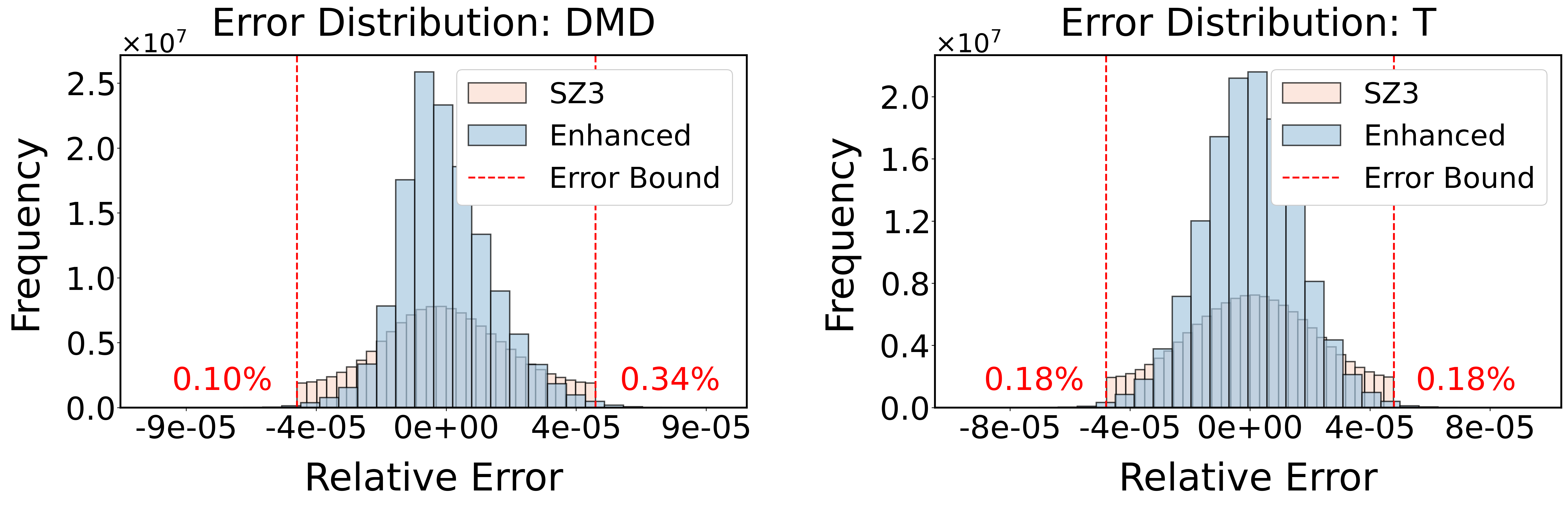
Figure 16. Error distribution for the Dark Matter Density (DMD) and Temperature (T) fields, comparing SZ3 decompressed and NeurLZ-initial-enhanced values to the original values under a 5E-5 relative error bound. The initial enhanced values exhibit outlier rates of 0.10% (lower bound) and 0.34% (upper bound) for DMD, and 0.18% (for both bounds) for T.

5.2. Uncovering Cross-Field Contributions: How Do Different Fields Contribute to Predictions?

Figure 5 demonstrates that cross-field learning results in a higher PSNR improvement compared to single-field learning. The information from multiple fields aids in achieving more accurate predictions, leading to better PSNR. However, understanding the specifics of how different fields contribute to this improvement is critical, particularly when predicting residual values for a specific datum. How much does each field contribute? Are all fields equally helpful? To uncover these cross-field contributions, we conducted an experiment for the Temperature field using the SZ3 compressor with a 5E-3 error bound. To enhance the Temperature field, we incorporated Dark Matter Density and Velocity X fields into the cross-field learning process. After 100 epochs, the trained model was analyzed using Captum, which applies integrated gradients for attribution analysis (Sundararajan et al., 2017; Kokhlikyan et al., 2020).

Given decompressed slices (512 $\times$ 512) from Temperature, Dark Matter Density, and Velocity X, the model predicted the residual slice for Temperature. We selected the datum at the (256, 256) position of the Temperature slice as the target for attribution analysis. Captum computed the attribution scores for each datum from the decompressed slices, quantifying the contribution of each datum in each field to the prediction of the residual value at the (256, 256) position in the Temperature field. Figure 17 presents the results. The top row shows the three slices from each field, with the target datum marked by a red star. The bottom row highlights the attribution regions for each field, with significant attribution areas emphasized by red rectangles for clearer visualization.

It can be observed that each field has a prominent red rectangle centered around the (256, 256) position, which corresponds to the datum being predicted. This highlights the local patterns across fields identified by NeurLZ, where each field’s local region near the predicted datum makes a significant contribution. In addition to these local patterns, global patterns also contribute to the prediction, as indicated by multiple smaller rectangles across the three fields. These regions demonstrate that global information from each field also plays a role in the prediction. It’s worth noting that the local and global patterns marked by the rectangles are not entirely consistent across the three fields, suggesting that each field contributes differently to the prediction. This visualization reveals that NeurLZ  leverages cross-field information through adaptable, learnable patterns, rather than fixed ones, resulting in improved PSNR.

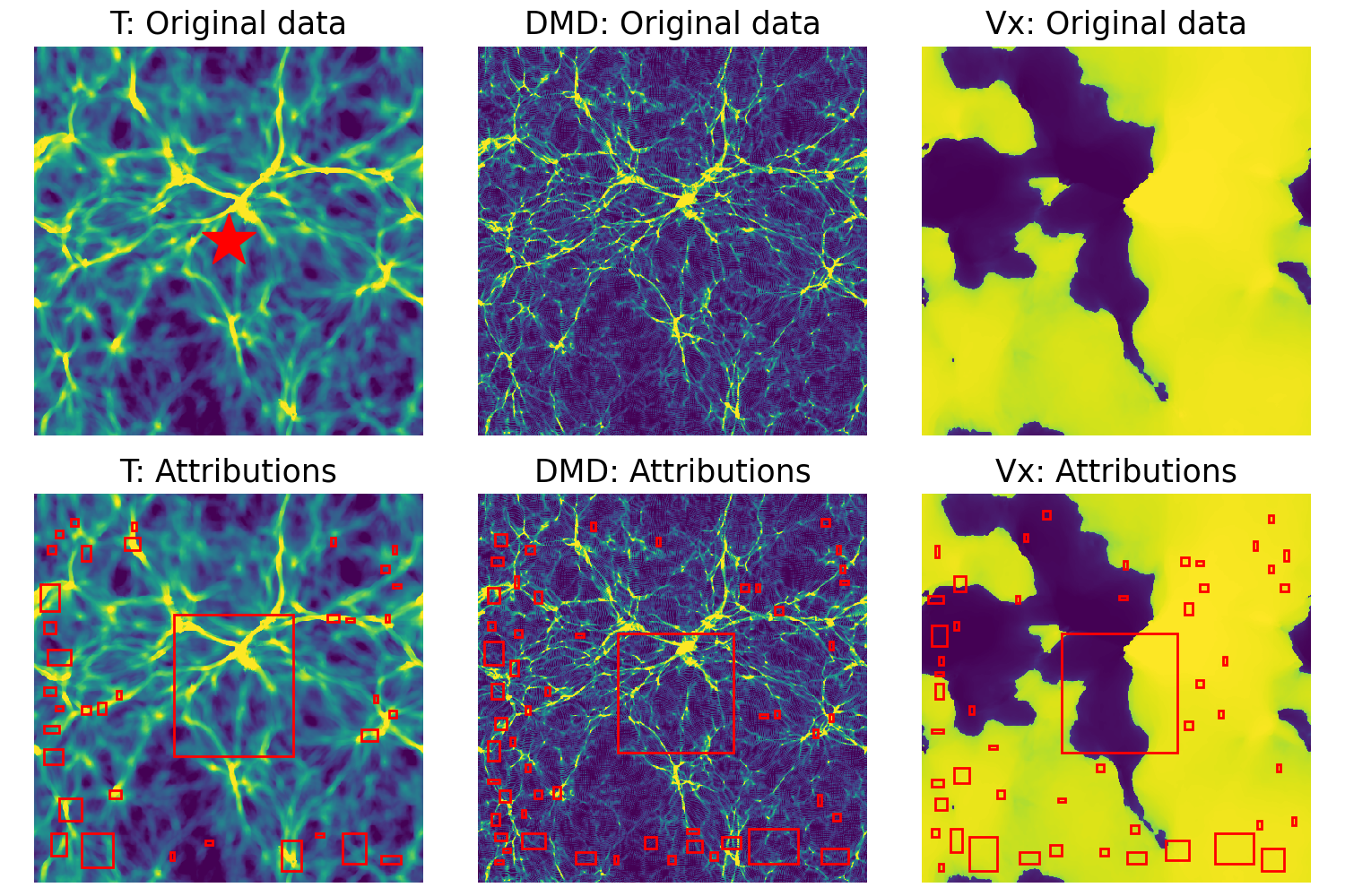
Figure 17. An visualization of cross-field learning: The top row shows three slices from the original data of three fields: T (Temperature), DMD (Dark Matter Density), and Vx (Velocity X). The bottom row displays the attribution regions for each field, highlighted with red rectangles, indicating areas with significant attribution values that contribute to the prediction at the (256, 256) position in the original data slice of T field, marked by a red star.

5.3. Understanding Performance Limitations: Does Conflict Hinder NeurLZ  at Stricter Error Bounds?

As discussed in Section 5, stricter error bounds generally result in diminished improvements from NeurLZ. For instance, the relative reduction in bit rate for the Velocity X field in the Nyx dataset is only 1.08% when NeurLZ  enhances SZ3 with an error bound of 1E-4, as shown in Table 2. In fact, with even stricter error bounds, such as 5E-5, NeurLZ  may not provide any improvement at all. Figure 18 illustrates the evolution of PSNR and outlier rate (OLR) (%) during training for the Velocity X field. Initially, the PSNR enhanced by NeurLZ  plateaus for the first 20 epochs before rapidly increasing and then becoming stagnant. Concurrently, the OLR increases as the enhanced PSNR improves, leading to a negative bit rate reduction, indicating that NeurLZ  may have a detrimental effect. This pattern of PSNR and OLR evolution contrasts with cases where NeurLZ  achieves significant improvements, as depicted in Figure 12. In these cases, PSNR increases while OLR decreases, resulting in overall relative reductions in bit rate of 66.4% and 36.3%. Overall, it seems that with stricter error bounds, NeurLZ  has less room for optimization. However, the question remains: why is there a performance limitation with stricter error bounds?

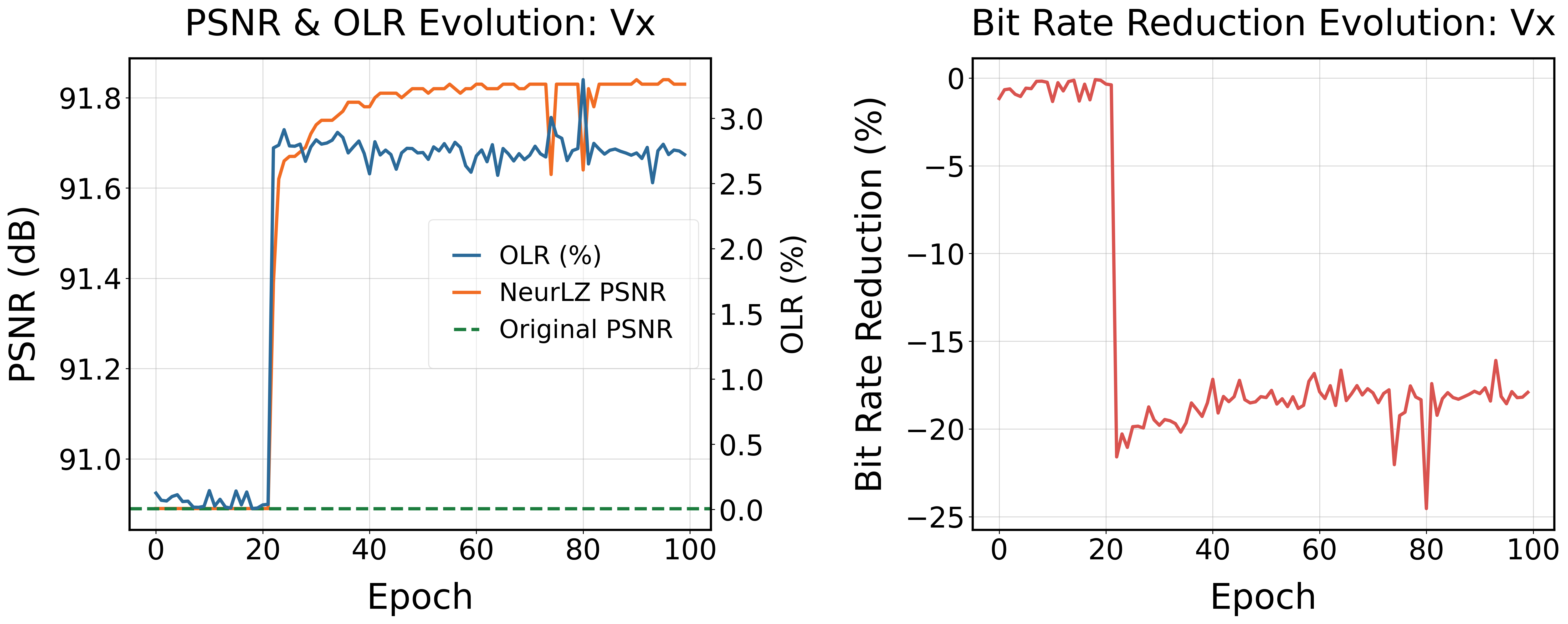
Figure 18. An illustration of the evolution of PSNR and outlier rate (OLR) (%) during training for the Velocity X (Vx) field in the Nyx dataset. PSNR was obtained using NeurLZ, which enhances the SZ3 compressor with a relative error bound of 5E-5. The sharp rise in PSNR and OLR, along with the drop in bit rate reduction, suggests that the skipping DNN model struggles to improve PSNR while keeping OLR low.

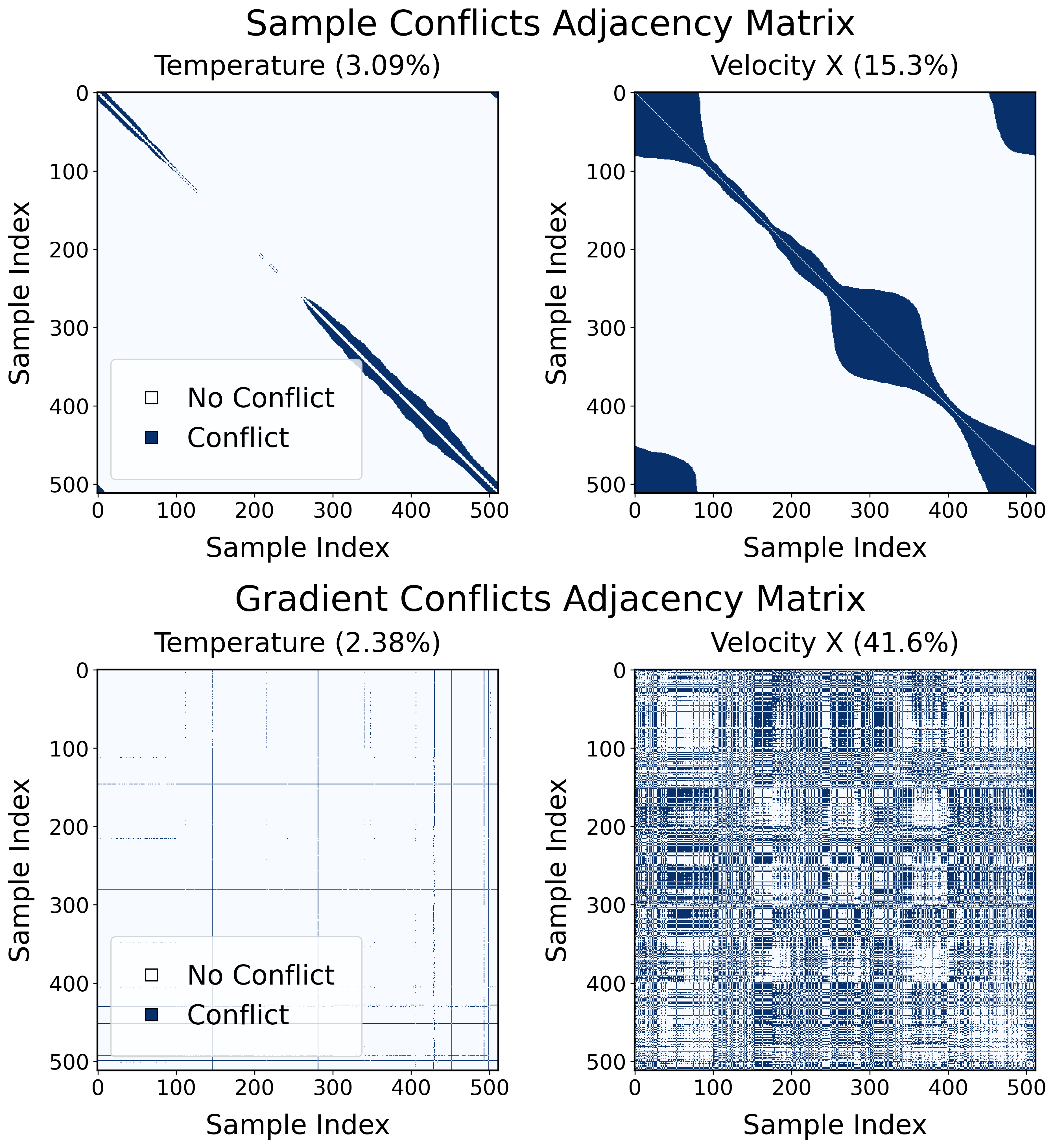
Figure 19. Sample conflicts (top) and gradient conflicts (bottom) adjacency matrices for Temperature and Velocity X fields in the Nyx dataset, each comprising 512 samples. Each sample forms a pair with every other sample, leading to a total of 262,144 pairs. The matrices depict conflict occurrences between these pairs. White areas (value 0) represent pairs without conflicts, while dark blue areas (value 1) indicate conflicting pairs. The subplot titles display the conflict proportions, quantifying the percentage of pairs exhibiting conflicts.

We hypothesize that the issue may stem from sample conflict, which introduce noise and hinder NeurLZ  at stricter error bounds. In certain situations, the input data $x_{1}$ and $x_{2}$ might be very similar, or even identical, but their corresponding desired outputs $y_{1}$ and $y_{2}$ are significantly different. Specifically, if $x_{1}\approx x_{2}$ or $x_{1}=x_{2}$, but at the same time $y_{1}\neq y_{2}$, it becomes very challenging for the model to learn effectively. We want the model to learn $f(x_{1})=y_{1}$ and $f(x_{2})=y_{2}$, but due to the similarity between $x_{1}$ and $x_{2}$, the model may struggle to distinguish between the two and generate the appropriate outputs. This phenomenon is often referred to as sample conflict. In such cases, it becomes difficult for the model to fit the training data properly, as it must generate different outputs for nearly identical inputs. Specifically, when $x_{1}\approx x_{2}$ and $y_{1}\neq y_{2}$, the model tends to map similar inputs to similar outputs, meaning $f(x_{1})\approx f(x_{2})$, which clearly conflicts with the goal of having $y_{1}\neq y_{2}$.

In our case, $x$ represents the decompressed slice, and $y$ represents the target field’s residual slice. For simplicity, we take the Nyx dataset’s Velocity X field under the SZ3 compressor as an example, using single-field learning. However, this analysis can also be extended to cross-field learning. Each decompressed slice, with a shape of 512 $\times$ 512, corresponds to an input $x$, while each residual slice, also with a shape of 512 $\times$ 512, corresponds to the output $y$. We can compute the similarity between different $x$ slices and between different $y$ slices, using the absolute value of cosine similarity as the metric. If the similarity between two decompressed slices, $x_{1}$ and $x_{2}$, exceeds 0.95 while the similarity between their corresponding residual slices, $y_{1}$ and $y_{2}$, is less than 0.05, we consider $(x_{1},y_{1})$ and $(x_{2},y_{2})$ to be in conflict. Otherwise, they are not considered as being in conflict.

The upper part of Figure 19 shows the sample conflict adjacency matrix. Since there are 512 $(x_{i},y_{i})$ pairs, the matrix has a shape of 512 $\times$ 512, representing a total of 262,144 pairwise comparisons for conflict calculation. The matrices depict the occurrence of conflicts between these pairs: white areas (value 0) indicate non-conflicting pairs, while dark blue areas (value 1) represent conflicting pairs. The subplot titles display the proportion of conflicts, quantifying the percentage of pairs exhibiting conflicts. In the left figure for Temperature, fewer conflicts are observed, with only 3.09% of the total pairs showing conflicts, compared to 15.3% for Velocity X. This aligns with the fact that Velocity X is more challenging to enhance. Interestingly, for both cases, most conflicts occur between neighboring slices, such as $(x_{i},y_{i})$ and $(x_{i+1},y_{i+1})$, which is visible as a dark blue region along the line $y=x$. This may be due to the decompressed values being smoother than the residual values, as the residuals tend to be more random. As a result, similar $x_{i}$ and $x_{i+1}$ values but different $y_{i}$ and $y_{i+1}$ values lead to conflicts.

The conflicts among samples can also lead to conflicting gradient updates during model training. We trained the models for 100 epochs and extracted the gradients for all 3,000 parameters for each sample, resulting in gradient vectors of size 3000 $\times$ 1. To analyze sample similarity based on gradients, we calculated the gradient conflict adjacency matrix. The lower part of Figure 19 presents the gradient conflict adjacency matrices for Temperature and Velocity X. Temperature exhibits a low conflict rate of 2.38%, indicating that most samples have similar gradient directions for updating model parameters. In contrast, Velocity X has a high conflict rate of 41.6%, suggesting that samples disagree on the optimal update directions. The differing proportions of conflicting gradient pairs among samples may contribute to the distinct training dynamics observed in Figure 12 and Figure 18. For Temperature, the consistent gradient directions lead to a smooth increase in PSNR and a decrease in OLR. However, for Velocity X, the conflicting gradients result in unstable increases in both PSNR and OLR, hindering model optimization. Overall, the observed sample and gradient conflicts limit model optimization, resulting in limited PSNR improvement and higher OLR, ultimately leading to diminished or even negative performance gains.

6. Conclusion

In this paper, we propose NeurLZ, an error-controlled compression framework based on neural learning. By utilizing skipping DNN models as lightweight enhancers incorporating cross-field learning, NeurLZ  significantly improves the quality of decompressed data reconstruction while maintaining excellent compression efficiency. The integrated error management ensures strict error control throughout the process. Experiments conducted on diverse datasets, including Nyx, Miranda, and Hurricane, demonstrate that NeurLZ achieves up to a 90% relative reduction in bit rate. To the best of our knowledge, NeurLZ is the first DNN-based, learn-to-compress, error-controlled framework.

References

- (1)
- Almgren et al. (2013) Ann S Almgren, John B Bell, Mike J Lijewski, Zarija Lukić, and Ethan Van Andel. 2013. Nyx: A massively parallel amr code for computational cosmology. The Astrophysical Journal 765, 1 (2013), 39.
- Chandak et al. (2020) Shubham Chandak, Kedar Tatwawadi, Chengtao Wen, Lingyun Wang, Juan Aparicio Ojea, and Tsachy Weissman. 2020. LFZip: Lossy compression of multivariate floating-point time series data via improved prediction. In 2020 Data Compression Conference (DCC). IEEE, 342–351.
- Collet and Kucherawy (2015) Yann Collet and EM Kucherawy. 2015. Zstandard-real-time data compression algorithm. Zstandard–real-time data compression algorithm (2015).
- Cook and Cabot (2024) Andrew Cook and William Cabot. 2024. Miranda Simulation Code. https://wci.llnl.gov/simulation/computer-codes/miranda. Accessed: [Date you accessed the site].
- Di and Cappello (2016) Sheng Di and Franck Cappello. 2016. Fast error-bounded lossy HPC data compression with SZ. In 2016 ieee international parallel and distributed processing symposium (ipdps). IEEE, 730–739.
- Di et al. (2024) Sheng Di, Jinyang Liu, Kai Zhao, Xin Liang, Robert Underwood, Zhaorui Zhang, Milan Shah, Yafan Huang, Jiajun Huang, Xiaodong Yu, et al. 2024. A Survey on Error-Bounded Lossy Compression for Scientific Datasets. arXiv preprint arXiv:2404.02840 (2024).
- Fan et al. (2022) Chi-Mao Fan, Tsung-Jung Liu, and Kuan-Hsien Liu. 2022. SUNet: Swin transformer UNet for image denoising. In 2022 IEEE International Symposium on Circuits and Systems (ISCAS). IEEE, 2333–2337.
- Gailly and Adler (2004) Jean-loup Gailly and Mark Adler. 2004. Zlib compression library. (2004).
- He et al. (2016) Kaiming He, Xiangyu Zhang, Shaoqing Ren, and Jian Sun. 2016. Deep residual learning for image recognition. In Proceedings of the IEEE conference on computer vision and pattern recognition. 770–778.
- Hu et al. (2019) Xiaodan Hu, Mohamed A Naiel, Alexander Wong, Mark Lamm, and Paul Fieguth. 2019. RUNet: A robust UNet architecture for image super-resolution. In Proceedings of the IEEE/CVF Conference on Computer Vision and Pattern Recognition Workshops. 0–0.
- Huffman (1952) David A Huffman. 1952. A method for the construction of minimum-redundancy codes. Proceedings of the IRE 40, 9 (1952), 1098–1101.
- Jia et al. (2024) Wenqi Jia, Sian Jin, Jinzhen Wang, Wei Niu, Dingwen Tao, and Miao Yin. 2024. GWLZ: A Group-wise Learning-based Lossy Compression Framework for Scientific Data. arXiv preprint arXiv:2404.13470 (2024).
- Kokhlikyan et al. (2020) Narine Kokhlikyan, Vivek Miglani, Miguel Martin, Edward Wang, Bilal Alsallakh, Jonathan Reynolds, Alexander Melnikov, Natalia Kliushkina, Carlos Araya, Siqi Yan, et al. 2020. Captum: A unified and generic model interpretability library for PyTorch. arXiv. arXiv preprint arXiv:2009.07896 (2020).
- Kokkinos and Lefkimmiatis (2018) Filippos Kokkinos and Stamatios Lefkimmiatis. 2018. Deep image demosaicking using a cascade of convolutional residual denoising networks. In Proceedings of the European conference on computer vision (ECCV). 303–319.
- Kong and Fu (2022) Yu Kong and Yun Fu. 2022. Human action recognition and prediction: A survey. International Journal of Computer Vision 130, 5 (2022), 1366–1401.
- Lakshminarasimhan et al. (2011) Sriram Lakshminarasimhan, Neil Shah, Stephane Ethier, Scott Klasky, Rob Latham, Rob Ross, and Nagiza F Samatova. 2011. Compressing the incompressible with ISABELA: In-situ reduction of spatio-temporal data. In Euro-Par 2011 Parallel Processing: 17th International Conference, Euro-Par 2011, Bordeaux, France, August 29-September 2, 2011, Proceedings, Part I 17. Springer, 366–379.
- Lakshminarasimhan et al. (2013) Sriram Lakshminarasimhan, Neil Shah, Stephane Ethier, Seung-Hoe Ku, Choong-Seock Chang, Scott Klasky, Rob Latham, Rob Ross, and Nagiza F Samatova. 2013. ISABELA for effective in situ compression of scientific data. Concurrency and Computation: Practice and Experience 25, 4 (2013), 524–540.
- Liang et al. (2019) Xin Liang, Sheng Di, Sihuan Li, Dingwen Tao, Bogdan Nicolae, Zizhong Chen, and Franck Cappello. 2019. Significantly improving lossy compression quality based on an optimized hybrid prediction model. In Proceedings of the International Conference for High Performance Computing, Networking, Storage and Analysis. 1–26.
- Liang et al. (2018) Xin Liang, Sheng Di, Dingwen Tao, Sihuan Li, Shaomeng Li, Hanqi Guo, Zizhong Chen, and Franck Cappello. 2018. Error-controlled lossy compression optimized for high compression ratios of scientific datasets. In 2018 IEEE International Conference on Big Data (Big Data). IEEE, 438–447.
- Liang et al. (2021) Xin Liang, Ben Whitney, Jieyang Chen, Lipeng Wan, Qing Liu, Dingwen Tao, James Kress, David Pugmire, Matthew Wolf, Norbert Podhorszki, et al. 2021. Mgard+: Optimizing multilevel methods for error-bounded scientific data reduction. IEEE Trans. Comput. 71, 7 (2021), 1522–1536.
- Liang et al. (2022) Xin Liang, Kai Zhao, Sheng Di, Sihuan Li, Robert Underwood, Ali M Gok, Jiannan Tian, Junjing Deng, Jon C Calhoun, Dingwen Tao, et al. 2022. Sz3: A modular framework for composing prediction-based error-bounded lossy compressors. IEEE Transactions on Big Data 9, 2 (2022), 485–498.
- Lindstrom (2014) Peter Lindstrom. 2014. Fixed-rate compressed floating-point arrays. IEEE transactions on visualization and computer graphics 20, 12 (2014), 2674–2683.
- Lindstrom and Isenburg (2006) Peter Lindstrom and Martin Isenburg. 2006. Fast and efficient compression of floating-point data. IEEE transactions on visualization and computer graphics 12, 5 (2006), 1245–1250.
- Lindstrom (2017) Peter G Lindstrom. 2017. Fpzip. Technical Report. Lawrence Livermore National Laboratory (LLNL), Livermore, CA (United States).
- Liu et al. (2023a) Jinyang Liu, Sheng Di, Sian Jin, Kai Zhao, Xin Liang, Zizhong Chen, and Franck Cappello. 2023a. SRN-SZ: Deep Leaning-Based Scientific Error-bounded Lossy Compression with Super-resolution Neural Networks. arXiv preprint arXiv:2309.04037 (2023).
- Liu et al. (2021) Jinyang Liu, Sheng Di, Kai Zhao, Sian Jin, Dingwen Tao, Xin Liang, Zizhong Chen, and Franck Cappello. 2021. Exploring autoencoder-based error-bounded compression for scientific data. In 2021 IEEE International Conference on Cluster Computing (CLUSTER). IEEE, 294–306.
- Liu et al. (2022) Jinyang Liu, Sheng Di, Kai Zhao, Xin Liang, Zizhong Chen, and Franck Cappello. 2022. Dynamic quality metric oriented error bounded lossy compression for scientific datasets. In SC22: International Conference for High Performance Computing, Networking, Storage and Analysis. IEEE, 1–15.
- Liu et al. (2023b) Jinyang Liu, Sheng Di, Kai Zhao, Xin Liang, Zizhong Chen, and Franck Cappello. 2023b. Faz: A flexible auto-tuned modular error-bounded compression framework for scientific data. In Proceedings of the 37th International Conference on Supercomputing. 1–13.
- Liu et al. (2023c) Jinyang Liu, Sheng Di, Kai Zhao, Xin Liang, Sian Jin, Zizhe Jian, Jiajun Huang, Shixun Wu, Zizhong Chen, and Franck Cappello. 2023c. High-performance Effective Scientific Error-bounded Lossy Compression with Auto-tuned Multi-component Interpolation. arXiv preprint arXiv:2311.12133 (2023).
- Liu et al. (2020) Li Liu, Wanli Ouyang, Xiaogang Wang, Paul Fieguth, Jie Chen, Xinwang Liu, and Matti Pietikäinen. 2020. Deep learning for generic object detection: A survey. International journal of computer vision 128 (2020), 261–318.
- Lukić et al. (2015) Zarija Lukić, Casey W Stark, Peter Nugent, Martin White, Avery A Meiksin, and Ann Almgren. 2015. The Lyman forest in optically thin hydrodynamical simulations. Monthly Notices of the Royal Astronomical Society 446, 4 (2015), 3697–3724.
- Mao et al. (2022) Yu Mao, Yufei Cui, Tei-Wei Kuo, and Chun Jason Xue. 2022. A fast transformer-based general-purpose lossless compressor. arXiv preprint arXiv:2203.16114 (2022).
- Oñorbe et al. (2019) Jose Oñorbe, FB Davies, Z Lukić, JF Hennawi, and D Sorini. 2019. Inhomogeneous reionization models in cosmological hydrodynamical simulations. Monthly Notices of the Royal Astronomical Society 486, 3 (2019), 4075–4097.
- Peter (1996) DEUTSCH Peter. 1996. GZIP file format specification version 4.3. Request for Comments: 1952 (1996).
- Rawat and Wang (2017) Waseem Rawat and Zenghui Wang. 2017. Deep convolutional neural networks for image classification: A comprehensive review. Neural computation 29, 9 (2017), 2352–2449.
- Rissanen and Langdon (1979) Jorma Rissanen and Glen G Langdon. 1979. Arithmetic coding. IBM Journal of research and development 23, 2 (1979), 149–162.
- Ronneberger et al. (2015) Olaf Ronneberger, Philipp Fischer, and Thomas Brox. 2015. U-net: Convolutional networks for biomedical image segmentation. In Medical image computing and computer-assisted intervention–MICCAI 2015: 18th international conference, Munich, Germany, October 5-9, 2015, proceedings, part III 18. Springer, 234–241.
- Shannon (1948) Claude Elwood Shannon. 1948. A mathematical theory of communication. The Bell system technical journal 27, 3 (1948), 379–423.
- Sundararajan et al. (2017) Mukund Sundararajan, Ankur Taly, and Qiqi Yan. 2017. Axiomatic attribution for deep networks. In International conference on machine learning. PMLR, 3319–3328.
- Tai et al. (2017) Ying Tai, Jian Yang, Xiaoming Liu, and Chunyan Xu. 2017. Memnet: A persistent memory network for image restoration. In Proceedings of the IEEE international conference on computer vision. 4539–4547.
- Tao et al. (2017) Dingwen Tao, Sheng Di, Zizhong Chen, and Franck Cappello. 2017. Significantly improving lossy compression for scientific data sets based on multidimensional prediction and error-controlled quantization. In 2017 IEEE International Parallel and Distributed Processing Symposium (IPDPS). IEEE, 1129–1139.
- Tao et al. (2019a) Dingwen Tao, Sheng Di, Hanqi Guo, Zizhong Chen, and Franck Cappello. 2019a. Z-checker: A framework for assessing lossy compression of scientific data. The International Journal of High Performance Computing Applications 33, 2 (2019), 285–303.
- Tao et al. (2019b) Dingwen Tao, Sheng Di, Xin Liang, Zizhong Chen, and Franck Cappello. 2019b. Optimizing lossy compression rate-distortion from automatic online selection between SZ and ZFP. IEEE Transactions on Parallel and Distributed Systems 30, 8 (2019), 1857–1871.
- Torbunov et al. (2023) Dmitrii Torbunov, Yi Huang, Haiwang Yu, Jin Huang, Shinjae Yoo, Meifeng Lin, Brett Viren, and Yihui Ren. 2023. Uvcgan: Unet vision transformer cycle-consistent gan for unpaired image-to-image translation. In Proceedings of the IEEE/CVF winter conference on applications of computer vision. 702–712.
- Torfi et al. (2020) Amirsina Torfi, Rouzbeh A Shirvani, Yaser Keneshloo, Nader Tavaf, and Edward A Fox. 2020. Natural language processing advancements by deep learning: A survey. arXiv preprint arXiv:2003.01200 (2020).
- Wang et al. (2020) Zhihao Wang, Jian Chen, and Steven CH Hoi. 2020. Deep learning for image super-resolution: A survey. IEEE transactions on pattern analysis and machine intelligence 43, 10 (2020), 3365–3387.
- Zhang et al. (2018) Haoran Zhang, Zhenzhen Hu, Changzhi Luo, Wangmeng Zuo, and Meng Wang. 2018. Semantic image inpainting with progressive generative networks. In Proceedings of the 26th ACM international conference on Multimedia. 1939–1947.
- Zhang et al. (2017) Kai Zhang, Wangmeng Zuo, Yunjin Chen, Deyu Meng, and Lei Zhang. 2017. Beyond a gaussian denoiser: Residual learning of deep cnn for image denoising. IEEE transactions on image processing 26, 7 (2017), 3142–3155.
- Zhao et al. (2021) Kai Zhao, Sheng Di, Maxim Dmitriev, Thierry-Laurent D Tonellot, Zizhong Chen, and Franck Cappello. 2021. Optimizing error-bounded lossy compression for scientific data by dynamic spline interpolation. In 2021 IEEE 37th International Conference on Data Engineering (ICDE). IEEE, 1643–1654.
- Zhao et al. (2020a) Kai Zhao, Sheng Di, Xin Lian, Sihuan Li, Dingwen Tao, Julie Bessac, Zizhong Chen, and Franck Cappello. 2020a. SDRBench: Scientific data reduction benchmark for lossy compressors. In 2020 IEEE international conference on big data (Big Data). IEEE, 2716–2724.
- Zhao et al. (2020b) Kai Zhao, Sheng Di, Xin Liang, Sihuan Li, Dingwen Tao, Zizhong Chen, and Franck Cappello. 2020b. Significantly improving lossy compression for HPC datasets with second-order prediction and parameter optimization. In Proceedings of the 29th International Symposium on High-Performance Parallel and Distributed Computing. 89–100.
- Ziv and Lempel (1977) Jacob Ziv and Abraham Lempel. 1977. A universal algorithm for sequential data compression. IEEE Transactions on information theory 23, 3 (1977), 337–343.