A discussion on estimating small bodies taxonomies using phase curves results

Abstract

Upcoming large multiwavelength photometric surveys will provide a leap in our understanding of small body populations, among other fields of modern astrophysics. Serendipitous observations of small bodies in different orbital locations allow us to study diverse phenomena related to how their surfaces scatter solar light.

In particular, multiple observations of the same object in different epochs permit us to construct their phase curves to obtain absolute magnitudes and phase coefficients. In this work, we tackle a series of long-used relationships associating these phase coefficients with the taxa of small bodies and suggest that some may need to be revised in the light of large-number statistics.

organization=Instituto de Astrofísica de Andalucía, CSIC,addressline=Apt 3004, city=Granada, postcode=E18080, country=Spain organization=Instituto de Física Aplicada a las Ciencias y las Tecnologías, Universidad de Alicante,addressline=San Vicent del Raspeig, E03080, city=Alicante, postcode=E03080, country=Spain

The geometric albedo vs. slope of the linear part of the phase curve relation may not hold to large numbers.

Taxonomy analyses from phase coefficients should be considered with care.

1 Introduction

Bobrovnikoff (1929) showed that asteroids do not only reflect light from the Sun but that light carries information from the surfaces, showing that not all asteroids’ surfaces are equal. Nevertheless, it was only in Chapman et al. (1975) that two broad groups with different reflectivity, i.e., colors, the S and C, were recognized. Further photometric analyses using multi-wavelength data re-identified the C and S major groupings while adding more details and generating the first taxonomies (see Tholen, 1984; Tholen and Barucci, 1989). The arrival of extensive photometric surveys, in particular the Sloan Digital Sky Survey’s Moving Objects Catalog (Ivezić et al., 2001; Jurić et al., 2002), further increased the details in the taxonomic distributions, but it kept the discrimination in two large complexes (see, for example, Carvano et al., 2010; Hasselmann et al., 2015; Colazo et al., 2022, and references therein) Certainly, spectroscopic data produce even more detailed taxonomic classifications (for example Bus and Binzel, 2002; DeMeo et al., 2009; Mahlke et al., 2022) but for the scope of this work, that level of detail is too large; therefore, we will only discuss photometric data in the remaining of this work.

The taxonomic classification is a proxy for the mineralogical properties of the surface of small bodies, hence its importance. The distribution of the taxa in the Solar System helps us understand the evolution that the Solar System suffered, not only from a dynamical point of view but also its physical-chemical evolution (for instance Gradie and Tedesco, 1982; Bell et al., 1989; Mothé-Diniz et al., 2003; DeMeo and Carry, 2013, 2014). The procedure to assign taxa uses colors obtained in a single observation (usually close in time if not simultaneous) or averages (weighted by uncertainties mostly) and different clustering techniques with convenient thresholds that define the borders between different groups; nevertheless, using a single observation or an average of the colors, although a valid approach when few data are available, turns out to increase the blur in borders between taxa due to phase coloring (Alvarez-Candal, 2024). Thus, we have been proposing a different approach: to determine the phase curves of the objects using multi-wavelength data from large surveys (Alvarez-Candal et al., 2022) and measure absolute colors, defined as the difference of absolute magnitudes in different filters (Ayala-Loera et al., 2018), to determine taxonomical classification.

The phase curve of asteroids shows the change of apparent brightness, normalized to unit distance from the Sun and the observer, with the phase angle $(\alpha$). The angle $\alpha$ is the angular distance subtended between the Sun and the observer, as seen from the object. The phase curves usually show an increasing behavior characterized by a linear change for $\alpha\geq 5-9$ deg, and a sudden increase in brightness at low-$\alpha$ (the opposition effect, Hapke 1963; Muinonen 1989).

To make the most of the information extracted from phase curves, we need to use a photometric model that describes the behavior of the magnitude (or flux) with $\alpha$ in the generic form

$$M(\alpha)=H+f(\vec{G},\vec{\Phi},\alpha),$$ (1)

where $H$ is the absolute magnitude, $\vec{G}$ are the phase coefficients, and $\vec{\Phi}$ are functions that describe the shape of the phase curve. In the simplest form, $f(\vec{G},\vec{\Phi},\alpha)=\beta\alpha$ and Eq. 1 is reduced to a linear approximation, which is often used with transneptunian objects because of their restricted phase angle coverage ($\alpha<2$ deg). In this work we will restrict to the HG₁G₂ (Muinonen et al., 2010) and the HG${}^{*}_{12}$ (Penttilä et al., 2016) photometric models. The former is the IAU-accepted model for small bodies, while the latter is an adaptation to work with lower-quality data or sparse coverage of the phase curves. A brief description of the models is given in Sect. 2. The procedure is to fit the best values of $\vec{G}$ and $H$ from the observed apparent magnitudes and phase angles.

The phase coefficients, which can be and have been used to estimate the taxa of asteroids, are usually linked to previous taxonomical classifications. This linkage makes sense as it provides a second use to data taken, generally, with other purposes, such as multi-epoch lightcurves or straight phase curve measurements. However, these studies are limited because the data used were taken in one or two photometric filters in traditional observing runs that maximize the observations for a limited sample of objects in a restricted span of phase angles. Yet, with the data produced by massive photometric surveys, it may be possible to use the phase curves to compute the absolute magnitudes necessary to estimate taxa without using the phase coefficients.

In the next Section, we will describe some of the limitations encountered in the literature with taxa estimation from phase curves. In contrast, in the final Section, we argue that multi-wavelength is the best approach. Although some of the results presented here were hinted at in previous works, this is the first time these issues are put forward in one place.

2 Issues of estimating taxa from phase curves

We need some background about the photometric models before describing the issues below. As mentioned above, we will use the HG₁G₂ and HG${}^{*}_{12}$ models. Muinonen et al. (2010) defined the first model as

$$f(\vec{G},\vec{\Phi},\alpha)=-2.5\log{[G_{1}\Phi_{1}(\alpha)+G_{2}\Phi_{2}(\alpha)+(1-G_{1}-G_{2})\Phi_{3}(\alpha)]},$$ (2)

where the $\Phi_{i}$ functions are tabulated. In their work, they proposed a version using a single phase coefficient G₁₂ such that G${}_{i}=$G_i(G₁₂), $i=1,2$, that worked better for a small number of observations. Later, Penttilä et al. (2016) proposed an improvement over the model with a new definition of the parametric approximations G${}_{i}=$G_i(G${}^{*}_{12}$), $i=1,2$, keeping the same form of the photometric model as shown in Eq. 2. Therefore, the reader should remember that G${}_{12}\neq$ G${}^{*}_{12}$.

2.1 Data

Most data presented in this work was obtained following the procedures described in Alvarez-Candal et al. (2022) and Alvarez-Candal (2024), unless explicitly mentioned.

To briefly describe the processing of the data: We used as input the data from the revision of the Sloan Digital Sky Survey by Sergeyev and Carry (2021). From the initial database, of more than $10^{6}$ observations of almost $4\times 10^{5}$ small bodies, we selected only objects with at least three observations and a minimum span of at least 5 deg in phase angle. The only quality cut applied was ignoring any data with photometric error more significant than 1 mag.

The processing of the data includes the probability distribution of the possible rotational light-curve amplitude of the object, as well as its rotational phase (see Eq. 3 in Alvarez-Candal 2024), which is then used to fit the photometric model of choice, see the following sections for details. The estimation of the phase coefficients is made by the computation of the complete probability distributions unless explicitly stated.

2.2 Single parametric model: G₁₂ and G${}_{12}^{*}$

Since the 80s’ it has been suggested that the average values of phase coefficients for different taxonomical types are different (Harris and Young, 1989) and can be used to estimate taxa. Note that, at the time, the photometric model used was the HG model (Bowell et al., 1989). Nevertheless, the usual uncertainties in the average values and the spread of each taxon in the phase coefficients phase space argue against a clear relation when analyzing massive numbers of phase curves (e.g., Oszkiewicz et al., 2012; Mahlke et al., 2021). Nevertheless, it must be noted that when using high-quality and well-covered phase curves of individual objects, differences in the shape of the phase curves are apparent (Shevchenko et al., 2016).

If the phase coefficients are good estimators of the small bodies taxa, they should show some relation with either wavelength and (or) the actual taxa of the objects. Therefore, we first analyze the possible dependence of the phase coefficients, in this case the parametric coefficient G₁₂ or G${}^{*}_{12}$, with these two.

Oszkiewicz et al. (2012) used results from her previous work (Oszkiewicz et al., 2011) on the phase curves of about half a million asteroids to study the relationship between the G₁₂ parameter and taxonomy. (Note that this work is previous to Penttilä et al. (2016) and therefore they did not use the G${}_{12}^{*}$.) The authors stated that it could be possible to compute the probability of an object having a given taxon according to its value of G₁₂, but that the distributions could be wide and overlapping (see Fig. 1 on their paper).

We repeated Oszkiewicz et al. (2012) analysis, but using our estimations of G${}_{12}^{*}$ (from Alvarez-Candal, 2024) and the taxonomy classification made by Colazo et al. (2022). The cross-match between these databases shows in total 3 196 objects classified as S-complex, 2 649 as C-complex, 2 209 as X-complex, and 1 142 as V-type. Figure 1, left panel, shows that the distributions of G${}_{12}^{*}$ are all similar, with mean values of 0.68, 0.70, 0.70, and 0.69 for the S, C, V, and X complexes, as defined in Colazo et al. (2022). The only notable feature in the distribution is the apparent extended tail of the V-complex, but we will not enter into details because this is out of the scope of this work.

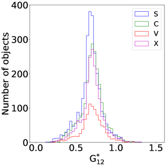
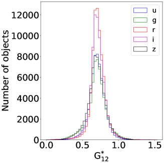
Figure 1: Distributions of G${}_{12}^{*}$. Left: The distributions for different taxa are shown in different colors. Right: The distributions for different filters are shown in different colors.

We also checked the possible variation of G${}_{12}^{*}$ with wavelength but found no evidence of it (see Fig. 1, right panel). The number of objects per filter is shown in Table 1.

Table 1: Number of objects. Columns 1, 4, and 7 indicate the photometric model used; columns 2, 5, and 8 indicate the photometric filter used. Colums 3, 6, and 9 indicate the number of phase curves fitted.

HG${}_{12}^{*}$	u	61 711	Lineal	u	14 877	HG1G2	V	3 819
	g	61 753	($\alpha>7.5$ deg)	g	16 008
	r	80 177		r	16 338
	i	80 196		i	16 331
	z	68 622		z	15 952
	all	42 168		all	17 387

2.3 Using G₁ and G₂

Using the parametric form of the phase coefficients permits the computation for scores of objects that cannot be fitted using the full HG₁G₂ model. The model needs a well-sampled phase curve and data with low-$\alpha$, below 3 degrees, to account for the opposition effect correctly. Nevertheless, studying what happens when using the model, even if it means working with fewer objects, is helpful.

Since the HG₁G₂ system was established in 2010 it was proposed a linear relation between the phase coefficients, G₁ and G₂ (see, for example, Muinonen et al., 2010; Shevchenko et al., 2016; Penttilä et al., 2016) where the different taxa more or less fall in different regions of the phase space (C-complex at high G₁ and low G₂, while S-complex at low G₁ and high G₂. E-type asteroids break this relation.) Although recent work by Arcoverde et al. (2023) on the phase curves of near-Earth asteroids does not show this distribution, showing, instead, a mix of objects with different taxa in different regions, new results obtained using ATLAS sparse data with dense data from ground-based telescopes support this view (Wilawer et al., 2024).

On the other hand, Mahlke et al. (2021) computed the phase curves in the cyan and orange filters of the Asteroid Terrestrial-impact Last Alert System, ATLAS, survey (Tonry et al., 2018) producing several tens of thousands of absolute magnitudes and phase coefficients. They created density plots for different taxa using G₁ and G₂ (see their work for details). From Fig. 6 in their paper, it is apparent that, although there are some differences at first glance, all taxa overlap significantly. Moreover, Dobson et al. (2023) fitted phase functions for a dozen transneptunian objects, centaurs, and Jupiter family comets. The authors could use the HG₁G₂ model for the ATLAS cyan and orange magnitudes for some of these objects. Whenever the values of G₁ and G₂ are plotted, with uncertainties, on top of Mahlke et al.’s regions, the values are compatible with all different taxonomical classes within one or two $\sigma$, meaning that the statistical difference between them is doubtful.

To check the accuracy of using G₁ and G₂ to estimate taxa, we use Mahlke’s database, selecting only the values of G₁ and G₂ obtained with the orange filter (the most numerous) to reconstruct the 2D maps. Instead of using all the taxonomical classes listed in Mahlke et al. (2021), we encompassed them into only four groups: 15 230 objects in the S-complex, 7 865 objects in the C-complex, 2 096 objects in the X-complex, and 2 009 objects in the V-complex (see Table 2 for details on how Mahlke’s taxa were divided into the complexes by Colazo et al. 2022). The reader should bear in mind that, due to the overall uncertainties in our data, we needed to make this simplification as we cannot yet detect the level of detail necessary to split our large complexes into smaller groups. We used the results from Shevchenko et al. (2016) to select a C-type and a S-type asteroid, with values G${}_{1}=0.76\pm 0.05$ and $0.30\pm 0.03$; and G${}_{2}=0.03\pm 0.03$ and $0.30\pm 0.03$, respectively. We also included a fictional object with G${}_{1}=0.50\pm 0.03$ and G${}_{2}=0.50\pm 0.03$ for comparison. Note that these values correspond to phase curves obtained in Johnson’s V filter, but for the sake of argument, we will assume they are all compatible with ATLAS’ orange filter. Figure 2 shows the phase space covered by the different complexes.

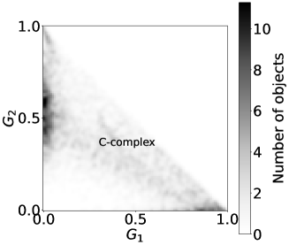
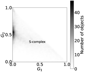
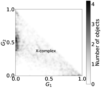
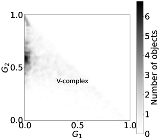
Figure 2: Heat maps of G₁ versus G₂. Each panel shows a different complex (see Table 2 for details).

Then, we wanted to answer the question: given the values of G_i of our test subjects, what are the probabilities of falling into one or more complex(es)? Therefore, we normalized each map to the total number of objects per map, and we created two-dimensional Gaussian profiles of each test object using the same binning as shown in Figs. 2 with the values of G_i mentioned above. To compute the probability of a given measurement belonging to each of the complexes, we just multiplied the Gaussian profile (also normalized to the unity area under the 2D curve) to each of the four maps. The results are: For the a priori C-type asteroid: C-complex 47 %, X-complex 45 %, S-complex 6 %, and V-complex 2 %; for the S-type asteroid: C-complex 55 %, S-complex 42 %, V-type 2 %, and X-complex 1 %. The generic asteroid has probabilities V-complex 32 %, X-complex 26 %, S-complex 22 %, and C-complex 20 %. From these figures, it is unclear that just one pair (G₁, G₂) could certify a taxonomical classification. However, the high-G₁, low-G₂ region seems to have a low probability of spectra with the 900 nm absorption band.

Table 2: Associated taxa

Complexa	Taxab
C	Cgh,Ch,B,F,FC,C,CB,CD,CF,CG,CL,CO,Cb,Cg,Cgx,Co,D,DP
S	K,L,LQ,Ld,S,SQ,SV,Sa,Sk,Sl,Sp,Sq,Sqw,Sr,Srw,Sv,Sw,A,AQ,Q,QO,QV
X	M,P,PC,PD,X,XC,XD,XL,Xc,Xe,Xk,Xt,E
V	O,V,Vw

^a Adapted from Colazo et al. (2022)
^b From Mahlke et al. (2021)

2.4 Geometrical albedoes and phase coefficients

Another parameter that enters into the taxonomic classification is the geometrical albedo of the objects. It is well-established that the C-complex and some X-complex objects tend to have low albedoes, while the S and V-complexes are associated with higher albedoes. Therefore, we checked whether using the albedo as an extra parameter in the G₁-G₂ space could distinguish among different kinds of objects.

We used our values of G₁ and G₂ computed from the data in Sergeyev and Carry (2021). We applied the HG₁G₂ model to all objects with at least three data, spanning a minimum of five degrees, and used the same methodology as in Alvarez-Candal (2024) only for the V filter. We obtained results for almost 4 000 objects (see Table 1). We cross-matched our results with the WISE albedoes (Mainzer et al., 2019). The cross-match provided almost 800 matches. The results are display in Fig. 3 separated in two samples: low-albedo ($p_{v}<0.1$) and high-albedo ($p_{v}>0.1$).

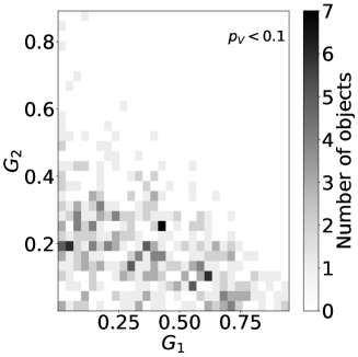
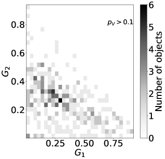
Figure 3: Heat map of G₁ versus G₂. The left panel shows objects with $p_{v}<0.1$, while the right panel shows $p_{v}>0.1$. Albedoes extracted from the WISE database.

There is no clear distinction among different albedoes in the figures, except perhaps a concentration of higher-albedoes objects towards values of G${}_{1}<0.5$, but the distribution generally seems reasonably uniform. In any case, these results should regarded with care because most of the phase curves have few points; nevertheless, there are about 350 objects with more than ten observations. Furthermore, on average, the results should not differ much from higher coverage phase curves, but a more thorough analysis is warranted when higher-quality data is available.

2.5 Relationship between albedo and the linear part of the phase curve

Regarding the use of albedoes and phase curve parameters, a significant relation that has been explored since Belskaya and Shevchenko (2000) put it forward is the apparent correlation found between the slope of the linear part of the phase curve, $h$, and albedo. The phase curves of small bodies have a linear behavior for $\alpha\gtrsim 7$ deg. The (anti) correlation seems like a strong result in the literature (see Fig. 4 in their work or, also Fig. 4, in Wilawer et al. 2022). Nevertheless, neither of these references reports the result of an actual correlation test. Moreover, scrutiny to Wilawer et al. (2022) data in Table 2 shows objects departing from apparent anticorrelation. These objects, the let-outs, have uncertainties more significant than 20 %, which are less precise values but not necessarily less accurate ones.

In Fig. 4, we show all objects in Wilawer et al. (2022) as they appear in their Table 2; in these cases of objects with more than one value, we selected the lower uncertainty to be as close as possible to their original criterion. The correlation disappears. Moreover, Spearman’s test shows that the null hypothesis cannot be rejected, i.e., that the quantities are uncorrelated.

A fair question is, what would happen if more data is added to the plot? Will the relation hold, dilute, or disappear? As in the previous Section, we used Sergeyev and Carry (2021)’s data to compute the $h$ for as many objects as possible. The selection criteria we used involved phase curves with at least 3 data, $\alpha_{min}>5.0$ deg, and a minimum span of 5 deg. We only used $m:\sigma_{m}\leq 1$ and the same method as in Alvarez-Candal (2024) but using a linear function as a photometric model. See the total numbers in Table 1. The outputs are the probability distributions of the slopes ($h$). The distributions of the almost 24 000 objects are available in the OSF folder https://osf.io/v2wkj/.

Using our $h$, we first matched the AKARI albedo list Alí-Lagoa et al. (2018) to our list, finding only 83 objects in common (see Fig. 4, left panel). We over-plot the data from Wilawer et al. (2022) as red points in the figure. Note that in the figure are only plotted objects with $h\leq 0.2$ mag per degree to match the range span from Wilawer et al. (2022). The Spearman test does not show evidence of correlation.

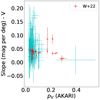
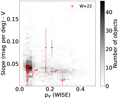
Figure 4: Left: Geometric albedo versus $h$. Albedoes from the AKARI mission. Right: Heat map of geometric albedo versus $h$. Albedoes from the WISE mission. The plot was cut for $p_{v}<0.5$ for clarity. Overplotted is Wilawer et al. (2022)’s data in red.

Still, the AKARI albedos do not cover the phase space Wilawer’s data covers. Note that only one datum has an albedo larger than 0.2.

Next, aiming at increasing the numbers, we cross-matched our $h$ with the albedos from the WISE mission (Mainzer et al., 2019), obtaining 4 122 matches. The comparison is shown in Fig. 4, right panel, where the data is displayed as a heat map to ease visualization. In this case, the Spearman test shows a weak anticorrelation with a $r_{s}=-0.2$. To explore how the uncertainty of the data may affect this anticorrelation, we generated 10 000 clones using normal distributions with $\sigma$ equal to the uncertainties in the $x$ and $y$ axes. The results of $r_{s}$ and $P_{r_{r}}$ are shown in Fig. 5 and indicate that a weak anticorrelation, most of the results cluster around $p_{r}\approx-0.06$ with very low $P_{r_{r}}$, may exist, implying steeper face curves tend to have lower-albedoes.

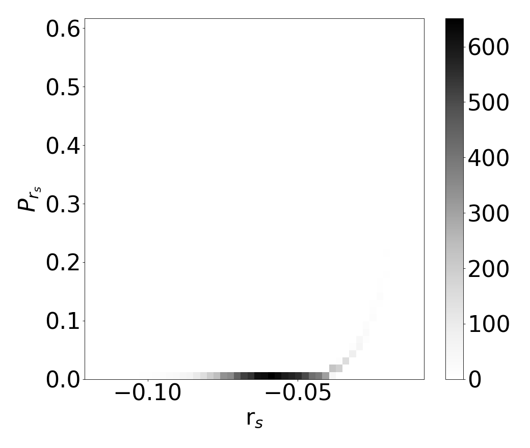
Figure 5: Distribution of the 10 000 Spearman test’ runs.

3 Taxonomy based on absolute colors

The above issues were raised not in an attempt to minimize the importance of previous (nor future) knowledge but to show that the upcoming flood of data, such as that from the Rubin Observatory’s Legacy Survey of Space and Time, LSST, will open up new avenues for improvement in the way we interpret data. This influx of data will not only change the way we look at current results but also provide the potential to reinterpret long-standing relations that may become blurred when more (a lot more) data is added.

In Alvarez-Candal et al. (2022), we presented absolute colors for over 14 000 objects. One of the objectives was to measure multi-wavelength absolute magnitudes to obtain the taxonomic classification of the objects ($>8\,000$ objects in Colazo et al., 2022). We extended this work for $>40\,000$ objects in Alvarez-Candal (2024), but a taxonomical classification is yet to be done. Indeed, this number is about only 10% of what we would get if using average colors or some other sorting algorithm. Therefore, is it worth the trouble to compute phase curves in multiple wavelengths? The answer is yes because the absolute colors are corrected by phase coloring, thus removing one possible bias. However, there may be issues when collating data from different apparitions. Nevertheless, the method used in Alvarez-Candal (2024) somehow includes this while computing the probability distribution $P_{A}(m,\Delta m)$ (see their Eqs. 3 and 4). It can be further improved. Moreover, we have shown in Alvarez-Candal et al. (2022) and Alvarez-Candal (2024) that using average colors biases the results towards low-$\alpha$ observations and that there is not a 1-1 relation between absolute colors and average colors; in fact, there is quite a large spread. Finally, in Alvarez-Candal (2024), we showed that the spectral slopes and colors of the objects do not follow the traditionally assumed reddening tendency with increasing $\alpha$. Moreover, two different kinds of photometric behavior that change at a critical angle of about 5 deg seem to exist (see also Wilawer et al. 2024). These behaviors are unrelated in any straightforward way to the actual taxa of the objects, size, or location in the Solar System.

As a side product, the absolute colors (or the respective relative reflectances) can be used as templates to study the phase effects because they provide the zero-phase angle benchmark and the effects of space weathering, providing uncolored templates.

4 Conclusions

This article highlights that estimating taxa from phase coefficients or relations based on small numbers of objects may not be ideal. The main problem when using phase curves is the need for more than one, in fact, a lot more than one, observations of the same object at different $\alpha$. Therefore, using phase angle-corrected colors to estimate taxa is less efficient than using single observations or averages, which do not have the risk of failing to fit a photometric model. Nevertheless, the near future seems bright, as the arrival of the LSST and its synergy with other large photometric surveys with similar photometric systems (for example the Dark Energy Survey, DES, Dark Energy Survey Collaboration et al. 2016, the Javalambre Physics of the Accelerating Universe Survey, J-PAS, Benitez et al. 2014; Bonoli et al. 2021, or the SkyMapper’s Southern Sky Survey, Wolf et al. 2018) will provide for observations of scores of objects in different $\alpha$ and epochs. Nevertheless, it is important to remember that, although similar, the photometric systems are not identical. Therefore, conversion relations must be used or developed, increasing the uncertainty budget.

Using absolute magnitudes to estimate taxa should eliminate some of the blur when different objects’ observations are used. There are some limitations to the method we have been developing; for instance, it tends to have larger uncertainties than traditional ones, such as averaging. However, we deal with complete probability distributions containing, if not all, at least most of the possible solutions within the current uncertainties of the observational data and rotational state of the object. As mentioned before, including more data from LSST or any other survey with a similar photometric system, or whose data can be transformed into SDSS-like, should improve the posterior distributions, increasing the precision of our absolute magnitudes, thus improving the taxonomical classification, which is free of phase angle effects.

References

- Alí-Lagoa et al. (2018) Alí-Lagoa, V., Müller, T.G., Usui, F., Hasegawa, S., 2018. The AKARI IRC asteroid flux catalogue: updated diameters and albedos. \aap 612, A85. doi:10.1051/0004-6361/201731806, arXiv:1712.07496.
- Alvarez-Candal (2024) Alvarez-Candal, A., 2024. The multiwavelength phase curves of small bodies. Phase coloring. \aap 685, A29. doi:10.1051/0004-6361/202348287, arXiv:2402.11113.
- Alvarez-Candal et al. (2022) Alvarez-Candal, A., Benavidez, P.G., Campo Bagatin, A., Santana-Ros, T., 2022. Phase curves of small bodies from the SLOAN Moving Objects Catalog. \aap 657, A80. doi:10.1051/0004-6361/202141033, arXiv:2110.06621.
- Arcoverde et al. (2023) Arcoverde, P., Rondón, E., Monteiro, F., Pereira, W., Ieva, S., Michtchenko, T., Evangelista-Santana, M., Michimani, J., Mesquita, W., Corrêa, T., Dotto, E., Giunta, A., Di Paola, A., Medeiros, H., Carvano, J.M., Rodrigues, T., Lazzaro, D., 2023. Physical properties of NEOs derived from their phase curves. \mnras 523, 739–757. doi:10.1093/mnras/stad1486.
- Ayala-Loera et al. (2018) Ayala-Loera, C., Alvarez-Candal, A., Ortiz, J.L., Duffard, R., Fernández-Valenzuela, E., Santos-Sanz, P., Morales, N., 2018. Absolute colours and phase coefficients of trans-Neptunian objects: HV - HR and relative phase coefficients. \mnras 481, 1848–1857. doi:10.1093/mnras/sty2363, arXiv:1808.09938.
- Bell et al. (1989) Bell, J.F., Davis, D.R., Hartmann, W.K., Gaffey, M.J., 1989. Asteroids: the big picture., in: Binzel, R.P., Gehrels, T., Matthews, M.S. (Eds.), Asteroids II, pp. 921–945.
- Belskaya and Shevchenko (2000) Belskaya, I.N., Shevchenko, V.G., 2000. Opposition Effect of Asteroids. \icarus 147, 94–105. doi:10.1006/icar.2000.6410.
- Benitez et al. (2014) Benitez, N., Dupke, R., Moles, M., Sodre, L., Cenarro, J., Marin-Franch, A., Taylor, K., Cristobal, D., Fernandez-Soto, A., Mendes de Oliveira, C., Cepa-Nogue, J., Abramo, L.R., Alcaniz, J.S., Overzier, R., Hernandez-Monteagudo, C., Alfaro, E.J., Kanaan, A., Carvano, J.M., Reis, R.R.R., Martinez Gonzalez, E., Ascaso, B., Ballesteros, F., Xavier, H.S., Varela, J., Ederoclite, A., Vazquez Ramio, H., Broadhurst, T., Cypriano, E., Angulo, R., Diego, J.M., Zandivarez, A., Diaz, E., Melchior, P., Umetsu, K., Spinelli, P.F., Zitrin, A., Coe, D., Yepes, G., Vielva, P., Sahni, V., Marcos-Caballero, A., Shu Kitaura, F., Maroto, A.L., Masip, M., Tsujikawa, S., Carneiro, S., Gonzalez Nuevo, J., Carvalho, G.C., Reboucas, M.J., Carvalho, J.C., Abdalla, E., Bernui, A., Pigozzo, C., Ferreira, E.G.M., Chandrachani Devi, N., Bengaly, C. A. P., J., Campista, M., Amorim, A., Asari, N.V., Bongiovanni, A., Bonoli, S., Bruzual, G., Cardiel, N., Cava, A., Cid Fernandes, R., Coelho, P., Cortesi, A., Delgado, R.G., Diaz Garcia, L., Espinosa, J.M.R., Galliano, E., Gonzalez-Serrano, J.I., Falcon-Barroso, J., Fritz, J., Fernandes, C., Gorgas, J., Hoyos, C., Jimenez-Teja, Y., Lopez-Aguerri, J.A., Lopez-San Juan, C., Mateus, A., Molino, A., Novais, P., OMill, A., Oteo, I., Perez-Gonzalez, P.G., Poggianti, B., Proctor, R., Ricciardelli, E., Sanchez-Blazquez, P., Storchi-Bergmann, T., Telles, E., Schoennell, W., Trujillo, N., Vazdekis, A., Viironen, K., Daflon, S., Aparicio-Villegas, T., Rocha, D., Ribeiro, T., Borges, M., Martins, S.L., Marcolino, W., Martinez-Delgado, D., Perez-Torres, M.A., Siffert, B.B., Calvao, M.O., Sako, M., Kessler, R., Alvarez-Candal, A., De Pra, M., Roig, F., Lazzaro, D., Gorosabel, J., Lopes de Oliveira, R., Lima-Neto, G.B., Irwin, J., Liu, J.F., Alvarez, E., Balmes, I., Chueca, S., Costa-Duarte, M.V., da Costa, A.A., Dantas, M.L.L., Diaz, A.Y., Fabregat, J., Ferrari, F., Gavela, B., Gracia, S.G., Gruel, N., Gutierrez, J.L.L., Guzman, R., Hernandez-Fernandez, J.D., Herranz, D., Hurtado-Gil, L., Jablonsky, F., Laporte, R., Le Tiran, L.L., Licandro, J., Lima, M., Martin, E., Martinez, V., Montero, J.J.C., Penteado, P., Pereira, C.B., Peris, V., Quilis, V., Sanchez-Portal, M., Soja, A.C., Solano, E., Torra, J., Valdivielso, L., 2014. J-PAS: The Javalambre-Physics of the Accelerated Universe Astrophysical Survey. arXiv e-prints , arXiv:1403.5237arXiv:1403.5237.
- Bobrovnikoff (1929) Bobrovnikoff, N.T., 1929. The spectra of minor planets. Lick Observatory Bulletin 407, 18–27. doi:10.5479/ADS/bib/1929LicOB.14.18B.
- Bonoli et al. (2021) Bonoli, S., Marín-Franch, A., Varela, J., Vázquez Ramió, H., Abramo, L.R., Cenarro, A.J., Dupke, R.A., Vílchez, J.M., Cristóbal-Hornillos, D., González Delgado, R.M., Hernández-Monteagudo, C., López-Sanjuan, C., Muniesa, D.J., Civera, T., Ederoclite, A., Hernán-Caballero, A., Marra, V., Baqui, P.O., Cortesi, A., Cypriano, E.S., Daflon, S., de Amorim, A.L., Díaz-García, L.A., Diego, J.M., Martínez-Solaeche, G., Pérez, E., Placco, V.M., Prada, F., Queiroz, C., Alcaniz, J., Alvarez-Candal, A., Cepa, J., Maroto, A.L., Roig, F., Siffert, B.B., Taylor, K., Benitez, N., Moles, M., Sodré, L., Carneiro, S., Mendes de Oliveira, C., Abdalla, E., Angulo, R.E., Aparicio Resco, M., Balaguera-Antolínez, A., Ballesteros, F.J., Brito-Silva, D., Broadhurst, T., Carrasco, E.R., Castro, T., Cid Fernandes, R., Coelho, P., de Melo, R.B., Doubrawa, L., Fernandez-Soto, A., Ferrari, F., Finoguenov, A., García-Benito, R., Iglesias-Páramo, J., Jiménez-Teja, Y., Kitaura, F.S., Laur, J., Lopes, P.A.A., Lucatelli, G., Martínez, V.J., Maturi, M., Overzier, R.A., Pigozzo, C., Quartin, M., Rodríguez-Martín, J.E., Salzano, V., Tamm, A., Tempel, E., Umetsu, K., Valdivielso, L., von Marttens, R., Zitrin, A., Díaz-Martín, M.C., López-Alegre, G., López-Sainz, A., Yanes-Díaz, A., Rueda-Teruel, F., Rueda-Teruel, S., Abril Ibañez, J., L Antón Bravo, J., Bello Ferrer, R., Bielsa, S., Casino, J.M., Castillo, J., Chueca, S., Cuesta, L., Garzarán Calderaro, J., Iglesias-Marzoa, R., Íniguez, C., Lamadrid Gutierrez, J.L., Lopez-Martinez, F., Lozano-Pérez, D., Maícas Sacristán, N., Molina-Ibáñez, E.L., Moreno-Signes, A., Rodríguez Llano, S., Royo Navarro, M., Tilve Rua, V., Andrade, U., Alfaro, E.J., Akras, S., Arnalte-Mur, P., Ascaso, B., Barbosa, C.E., Beltrán Jiménez, J., Benetti, M., Bengaly, C.A.P., Bernui, A., Blanco-Pillado, J.J., Borges Fernandes, M., Bregman, J.N., Bruzual, G., Calderone, G., Carvano, J.M., Casarini, L., Chaves-Montero, J., Chies-Santos, A.L., Coutinho de Carvalho, G., Dimauro, P., Duarte Puertas, S., Figueruelo, D., González-Serrano, J.I., Guerrero, M.A., Gurung-López, S., Herranz, D., Huertas-Company, M., Irwin, J.A., Izquierdo-Villalba, D., Kanaan, A., Kehrig, C., Kirkpatrick, C.C., Lim, J., Lopes, A.R., Lopes de Oliveira, R., Marcos-Caballero, A., Martínez-Delgado, D., Martínez-González, E., Martínez-Somonte, G., Oliveira, N., Orsi, A.A., Penna-Lima, M., Reis, R.R.R., Spinoso, D., Tsujikawa, S., Vielva, P., Vitorelli, A.Z., Xia, J.Q., Yuan, H.B., Arroyo-Polonio, A., Dantas, M.L.L., Galarza, C.A., Gonçalves, D.R., Gonçalves, R.S., Gonzalez, J.E., Gonzalez, A.H., Greisel, N., Jiménez-Esteban, F., Landim, R.G., Lazzaro, D., Magris, G., Monteiro-Oliveira, R., Pereira, C.B., Rebouças, M.J., Rodriguez-Espinosa, J.M., Santos da Costa, S., Telles, E., 2021. The miniJPAS survey: A preview of the Universe in 56 colors. \aap 653, A31. doi:10.1051/0004-6361/202038841, arXiv:2007.01910.
- Bowell et al. (1989) Bowell, E., Hapke, B., Domingue, D., Lumme, K., Peltoniemi, J., Harris, A.W., 1989. Application of photometric models to asteroids., in: Binzel, R.P., Gehrels, T., Matthews, M.S. (Eds.), Asteroids II, pp. 524–556.
- Bus and Binzel (2002) Bus, S.J., Binzel, R.P., 2002. Phase II of the Small Main-Belt Asteroid Spectroscopic Survey. A Feature-Based Taxonomy. \icarus 158, 146–177. doi:10.1006/icar.2002.6856.
- Carry et al. (2024) Carry, B., Peloton, J., Le Montagner, R., Mahlke, M., Berthier, J., 2024. Combined spin orientation and phase function of asteroids. arXiv e-prints , arXiv:2403.20179doi:10.48550/arXiv.2403.20179, arXiv:2403.20179.
- Carvano et al. (2010) Carvano, J.M., Hasselmann, P.H., Lazzaro, D., Mothé-Diniz, T., 2010. SDSS-based taxonomic classification and orbital distribution of main belt asteroids. \aap 510, A43. doi:10.1051/0004-6361/200913322.
- Chapman et al. (1975) Chapman, C.R., Morrison, D., Zellner, B., 1975. Surface Properties of Asteroids: A Synthesis of Polarimetry, Radiometry, and Spectrophotometry. \icarus 25, 104–130. doi:10.1016/0019-1035(75)90191-8.
- Colazo et al. (2022) Colazo, M., Alvarez-Candal, A., Duffard, R., 2022. Zero-phase angle asteroid taxonomy classification using unsupervised machine learning algorithms. \aap 666, A77. doi:10.1051/0004-6361/202243428, arXiv:2204.05075.
- Dark Energy Survey Collaboration et al. (2016) Dark Energy Survey Collaboration, Abbott, T., Abdalla, F.B., Aleksić, J., Allam, S., Amara, A., Bacon, D., Balbinot, E., Banerji, M., Bechtol, K., Benoit-Lévy, A., Bernstein, G.M., Bertin, E., Blazek, J., Bonnett, C., Bridle, S., Brooks, D., Brunner, R.J., Buckley-Geer, E., Burke, D.L., Caminha, G.B., Capozzi, D., Carlsen, J., Carnero-Rosell, A., Carollo, M., Carrasco-Kind, M., Carretero, J., Castander, F.J., Clerkin, L., Collett, T., Conselice, C., Crocce, M., Cunha, C.E., D’Andrea, C.B., da Costa, L.N., Davis, T.M., Desai, S., Diehl, H.T., Dietrich, J.P., Dodelson, S., Doel, P., Drlica-Wagner, A., Estrada, J., Etherington, J., Evrard, A.E., Fabbri, J., Finley, D.A., Flaugher, B., Foley, R.J., Fosalba, P., Frieman, J., García-Bellido, J., Gaztanaga, E., Gerdes, D.W., Giannantonio, T., Goldstein, D.A., Gruen, D., Gruendl, R.A., Guarnieri, P., Gutierrez, G., Hartley, W., Honscheid, K., Jain, B., James, D.J., Jeltema, T., Jouvel, S., Kessler, R., King, A., Kirk, D., Kron, R., Kuehn, K., Kuropatkin, N., Lahav, O., Li, T.S., Lima, M., Lin, H., Maia, M.A.G., Makler, M., Manera, M., Maraston, C., Marshall, J.L., Martini, P., McMahon, R.G., Melchior, P., Merson, A., Miller, C.J., Miquel, R., Mohr, J.J., Morice-Atkinson, X., Naidoo, K., Neilsen, E., Nichol, R.C., Nord, B., Ogando, R., Ostrovski, F., Palmese, A., Papadopoulos, A., Peiris, H.V., Peoples, J., Percival, W.J., Plazas, A.A., Reed, S.L., Refregier, A., Romer, A.K., Roodman, A., Ross, A., Rozo, E., Rykoff, E.S., Sadeh, I., Sako, M., Sánchez, C., Sanchez, E., Santiago, B., Scarpine, V., Schubnell, M., Sevilla-Noarbe, I., Sheldon, E., Smith, M., Smith, R.C., Soares-Santos, M., Sobreira, F., Soumagnac, M., Suchyta, E., Sullivan, M., Swanson, M., Tarle, G., Thaler, J., Thomas, D., Thomas, R.C., Tucker, D., Vieira, J.D., Vikram, V., Walker, A.R., Wechsler, R.H., Weller, J., Wester, W., Whiteway, L., Wilcox, H., Yanny, B., Zhang, Y., Zuntz, J., 2016. The Dark Energy Survey: more than dark energy - an overview. \mnras 460, 1270–1299. doi:10.1093/mnras/stw641, arXiv:1601.00329.
- DeMeo et al. (2009) DeMeo, F.E., Binzel, R.P., Slivan, S.M., Bus, S.J., 2009. An extension of the Bus asteroid taxonomy into the near-infrared. \icarus 202, 160–180. doi:10.1016/j.icarus.2009.02.005.
- DeMeo and Carry (2013) DeMeo, F.E., Carry, B., 2013. The taxonomic distribution of asteroids from multi-filter all-sky photometric surveys. \icarus 226, 723–741. doi:10.1016/j.icarus.2013.06.027, arXiv:1307.2424.
- DeMeo and Carry (2014) DeMeo, F.E., Carry, B., 2014. Solar System evolution from compositional mapping of the asteroid belt. \nat 505, 629–634. doi:10.1038/nature12908, arXiv:1408.2787.
- Dobson et al. (2023) Dobson, M.M., Schwamb, M.E., Benecchi, S.D., Verbiscer, A.J., Fitzsimmons, A., Shingles, L.J., Denneau, L., Heinze, A.N., Smith, K.W., Tonry, J.L., Weiland, H., Young, D.R., 2023. Phase Curves of Kuiper Belt Objects, Centaurs, and Jupiter-family Comets from the ATLAS Survey. \psj 4, 75. doi:10.3847/PSJ/acc463, arXiv:2303.08643.
- Gradie and Tedesco (1982) Gradie, J., Tedesco, E., 1982. Compositional Structure of the Asteroid Belt. Science 216, 1405–1407. doi:10.1126/science.216.4553.1405.
- Hapke (1963) Hapke, B.W., 1963. A theoretical photometric function for the lunar surface. \jgr 68, 4571–4586. doi:10.1029/JZ068i015p04571.
- Harris and Young (1989) Harris, A.W., Young, J.W., 1989. Asteroid lightcurve observations from 1979-1981. \icarus 81, 314–364. doi:10.1016/0019-1035(89)90056-0.
- Hasselmann et al. (2015) Hasselmann, P.H., Fulchignoni, M., Carvano, J.M., Lazzaro, D., Barucci, M.A., 2015. Characterizing spectral continuity in SDSS u’g’r’i’z’ asteroid photometry. \aap 577, A147. doi:10.1051/0004-6361/201424620, arXiv:1710.01180.
- Ivezić et al. (2001) Ivezić, Ž., Tabachnik, S., Rafikov, R., Lupton, R.H., Quinn, T., Hammergren, M., Eyer, L., Chu, J., Armstrong, J.C., Fan, X., Finlator, K., Geballe, T.R., Gunn, J.E., Hennessy, G.S., Knapp, G.R., Leggett, S.K., Munn, J.A., Pier, J.R., Rockosi, C.M., Schneider, D.P., Strauss, M.A., Yanny, B., Brinkmann, J., Csabai, I., Hindsley, R.B., Kent, S., Lamb, D.Q., Margon, B., McKay, T.A., Smith, J.A., Waddel, P., York, D.G., SDSS Collaboration, 2001. Solar System Objects Observed in the Sloan Digital Sky Survey Commissioning Data. \aj 122, 2749–2784. doi:10.1086/323452, arXiv:astro-ph/0105511.
- Jurić et al. (2002) Jurić, M., Ivezić, Ž., Lupton, R.H., Quinn, T., Tabachnik, S., Fan, X., Gunn, J.E., Hennessy, G.S., Knapp, G.R., Munn, J.A., Pier, J.R., Rockosi, C.M., Schneider, D.P., Brinkmann, J., Csabai, I., Fukugita, M., 2002. Comparison of Positions and Magnitudes of Asteroids Observed in the Sloan Digital Sky Survey with Those Predicted for Known Asteroids. \aj 124, 1776–1787. doi:10.1086/341950, arXiv:astro-ph/0202468.
- Mahlke et al. (2021) Mahlke, M., Carry, B., Denneau, L., 2021. Asteroid phase curves from ATLAS dual-band photometry. \icarus 354, 114094. doi:10.1016/j.icarus.2020.114094, arXiv:2009.05129.
- Mahlke et al. (2022) Mahlke, M., Carry, B., Mattei, P.A., 2022. Asteroid taxonomy from cluster analysis of spectrometry and albedo. \aap 665, A26. doi:10.1051/0004-6361/202243587, arXiv:2203.11229.
- Mainzer et al. (2019) Mainzer, A.K., Bauer, J.M., Cutri, R.M., Grav, T., Kramer, E.A., Masiero, J.R., Sonnett, S., Wright, E.L., 2019. NEOWISE Diameters and Albedos V2.0. NASA Planetary Data System doi:10.26033/18S3-2Z54.
- Mothé-Diniz et al. (2003) Mothé-Diniz, T., Carvano, J.M.á., Lazzaro, D., 2003. Distribution of taxonomic classes in the main belt of asteroids. \icarus 162, 10–21. doi:10.1016/S0019-1035(02)00066-0.
- Muinonen (1989) Muinonen, K., 1989. Scattering of light by crystals: a modified Kirchhoff approximation. \ao 28, 3044–3050. doi:10.1364/AO.28.003044.
- Muinonen et al. (2010) Muinonen, K., Belskaya, I.N., Cellino, A., Delbò, M., Levasseur-Regourd, A.C., Penttilä, A., Tedesco, E.F., 2010. A three-parameter magnitude phase function for asteroids. \icarus 209, 542–555. doi:10.1016/j.icarus.2010.04.003.
- Oszkiewicz et al. (2011) Oszkiewicz, D., Muinonen, K., Bowell, E., Trilling, D., Penttilä, A., Pieniluoma, T., Wasserman, L., Enga, M.T., 2011. Online multi-parameter phase-curve fitting and application to a large corpus of asteroid photometric data. Journal of Quantitative Spectroscopy and Radiative Transfer 112, 1919–1929. URL: https://www.sciencedirect.com/science/article/pii/S0022407311001130, doi:https://doi.org/10.1016/j.jqsrt.2011.03.003. electromagnetic and Light Scattering by Nonspherical Particles XII.
- Oszkiewicz et al. (2012) Oszkiewicz, D.A., Bowell, E., Wasserman, L.H., Muinonen, K., Penttilä, A., Pieniluoma, T., Trilling, D.E., Thomas, C.A., 2012. Asteroid taxonomic signatures from photometric phase curves. \icarus 219, 283–296. doi:10.1016/j.icarus.2012.02.028, arXiv:1202.2270.
- Penttilä et al. (2016) Penttilä, A., Shevchenko, V.G., Wilkman, O., Muinonen, K., 2016. H, G1, G2 photometric phase function extended to low-accuracy data. \planss 123, 117–125. doi:10.1016/j.pss.2015.08.010.
- Sergeyev and Carry (2021) Sergeyev, A.V., Carry, B., 2021. A million asteroid observations in the Sloan Digital Sky Survey. \aap 652, A59. doi:10.1051/0004-6361/202140430, arXiv:2108.05749.
- Shevchenko et al. (2016) Shevchenko, V.G., Belskaya, I.N., Muinonen, K., Penttilä, A., Krugly, Y.N., Velichko, F.P., Chiorny, V.G., Slyusarev, I.G., Gaftonyuk, N.M., Tereschenko, I.A., 2016. Asteroid observations at low phase angles. IV. Average parameters for the new H, G1, G2 magnitude system. \planss 123, 101–116. doi:10.1016/j.pss.2015.11.007.
- Tholen (1984) Tholen, D.J., 1984. Asteroid Taxonomy from Cluster Analysis of Photometry. Ph.D. thesis. University of Arizona.
- Tholen and Barucci (1989) Tholen, D.J., Barucci, M.A., 1989. Asteroid taxonomy., in: Binzel, R.P., Gehrels, T., Matthews, M.S. (Eds.), Asteroids II, pp. 298–315.
- Tonry et al. (2018) Tonry, J.L., Denneau, L., Heinze, A.N., Stalder, B., Smith, K.W., Smartt, S.J., Stubbs, C.W., Weiland, H.J., Rest, A., 2018. ATLAS: A High-cadence All-sky Survey System. \pasp 130, 064505. doi:10.1088/1538-3873/aabadf, arXiv:1802.00879.
- Wilawer et al. (2024) Wilawer, E., Muinonen, K., Oszkiewicz, D., Kryszczyńska, A., Colazo, M., 2024. Phase curve wavelength dependency as revealed by shape- and geometry- corrected asteroid phase curves. \mnras 531, 2802–2816. doi:10.1093/mnras/stae1282.
- Wilawer et al. (2022) Wilawer, E., Oszkiewicz, D., Kryszczyńska, A., Marciniak, A., Shevchenko, V., Belskaya, I., Kwiatkowski, T., Kankiewicz, P., Horbowicz, J., Kudak, V., Kulczak, P., Perig, V., Sobkowiak, K., 2022. Asteroid phase curves using sparse Gaia DR2 data and differential dense light curves. Monthly Notices of the Royal Astronomical Society 513, 3242–3251. URL: https://doi.org/10.1093/mnras/stac1008, doi:10.1093/mnras/stac1008, arXiv:https://academic.oup.com/mnras/article-pdf/513/3/3242/43668322/stac1008.pdf.
- Wolf et al. (2018) Wolf, C., Onken, C.A., Luvaul, L.C., Schmidt, B.P., Bessell, M.S., Chang, S.W., Da Costa, G.S., Mackey, D., Martin-Jones, T., Murphy, S.J., Preston, T., Scalzo, R.A., Shao, L., Smillie, J., Tisserand, P., White, M.C., Yuan, F., 2018. SkyMapper Southern Survey: First Data Release (DR1). \pasa 35, e010. doi:10.1017/pasa.2018.5, arXiv:1801.07834.