Are Heterophilic GNNs and Homophily Metrics Really Effective? Evaluation Pitfalls and New Benchmarks

Abstract

Over the past decade, Graph Neural Networks (GNNs) have achieved great success on machine learning tasks with relational data. However, recent studies have found that heterophily can cause significant performance degradation of GNNs, especially on node-level tasks. Numerous heterophilic benchmark datasets have been put forward to validate the efficacy of heterophily-specific GNNs and various homophily metrics have been designed to help people recognize these malignant datasets. Nevertheless, there still exist multiple pitfalls that severely hinder the proper evaluation of new models and metrics. In this paper, we point out three most serious pitfalls: 1) a lack of hyperparameter tuning; 2) insufficient model evaluation on the real challenging heterophilic datasets; 3) missing quantitative evaluation benchmark for homophily metrics on synthetic graphs. To overcome these challenges, we first train and fine-tune baseline models on $27$ most widely used benchmark datasets, categorize them into three distinct groups: malignant, benign and ambiguous heterophilic datasets, and identify the real challenging subsets of tasks. To our best knowledge, we are the first to propose such taxonomy. Then, we re-evaluate $10$ heterophily-specific state-of-the-arts (SOTA) GNNs with fine-tuned hyperparameters on different groups of heterophilic datasets. Based on the model performance, we reassess their effectiveness on addressing heterophily challenge. At last, we evaluate $11$ popular homophily metrics on synthetic graphs with three different generation approaches. To compare the metrics strictly, we propose the first quantitative evaluation method based on Fréchet distance.

1 Introduction

As a generic data structure, graph is capable of modeling complex relations among objects in many real-world problems [1, 2, 3, 4]. In the last decade, various Graph Neural Networks (GNNs) architectures have been proposed [5, 6, 7, 8, 9, 10, 11, 12, 13] and shown to outperform traditional neural networks (NNs) in modeling graph-based real-world tasks [14, 15, 16, 17, 18, 19, 20].

The success of GNNs, especially on node-level tasks, is commonly believed to be rooted in the homophily principle [21], which means that connected nodes are more likely to have similar labels [22] or attributes [23]. Such inductive bias is thought to be a major contributor to the superiority of GNNs over NNs on various tasks [24]. On the other hand, the lack of homophily, i.e., heterophily [25, 26], is considered as the main cause of the inferiority of GNNs on heterophilic graphs, because heterophilic edges connect nodes between different classes, which can lead to mixed and indistinguishable node embeddings in message passing process [24, 27]. Recently, numerous models have been proposed to address the heterophily challenge [22, 24, 27, 28, 29, 30, 31, 32, 33, 34, 35, 26] and many homophily metrics have been put forward to identify the graph datasets that are unfriendly to GNNs [26, 36].

However, there is currently no work attempting to validate the effectiveness of the recent advances in heterophilic graph representation learning. Upon examination, we empirically find that there exist several pitfalls that can severely impede fair and accurate assessment of models and metrics:

• Lacking Enough Hyperparameter Tuning. Sufficient hyperparameter tuning is critical for reliable evaluation and fair comparison between models, and it also applies to heterophily-specific GNNs. With careful hyperparameter tuning, it is empirically found that basic GNNs can actually outperform some heterophily-specific models on several heterophilic graphs [37]. Through experiments we have found that, even on the datasets where the baseline models are claimed to be quite robust to the hyperparameter selection, tuning hyperparameters in a sufficiently large range can still make a significant difference to model performance. This indicates that there potentially exist a substantial amount of inaccurate and biased results reported in current literature, which mislead our understanding of heterophily problem. A fair model re-evaluation with careful hyperparameter fine-tuning is urgently needed.

• Insufficient Evaluation on The Real Challenging Heterophilic Datasets. Based on the studies in [37, 38, 39], the real challenging heterophilic datasets are those where graph-aware models underperform graph-agnostic models, instead of those with small homophily values. With this criterion, many of the commonly used heterophilic benchmark datasets cannot represent the real difficult heterophily tasks. Therefore, the evaluation results from these datasets cannot adequately demonstrate the effectiveness of newly proposed GNNs in handling heterophily.

• Absence of Quantitative Evaluation Benchmark for Homophily Metrics. The existing evaluation methods for homophily metrics mostly include these steps: 1) generate synthetic graphs with different levels of homophily-related parameters, e.g., edge homophily [34] and homophily coefficient [40]; 2) for each synthetic graph, we calculate the metric values and fine-tune baseline GNNs; 3) plot metric curves and GNN performance curves w.r.t. the homophily-related parameters, observe and compare the correlation between metric curves and GNN performance curves. However, such observation-based comparison can easily lead us to biased and inaccurate conclusions and there is no quantitative benchmark to evaluate homophily metrics.

In this paper, we aim to address the above issues for heterophilic graph learning and our main contributions are:

• Fine-tune Baseline Models and Discover Malignant, Benign and Ambiguous Heterophily Datasets. To find out the real challenging heterophilic datasets, in Section 3.3, we fine-tune graph-aware models and their corresponding graph-agnostic models on $27$ most used benchmark datasets. We find that there exist three disjoint sets of heterophilic datasets, where graph-aware models: 1) consistently outperform graph-aware models; 2) consistently underperform graph-aware models; 3) have inconsistent performance against graph-aware models. Based on this discovery, we categorize them into three types of heterophilic graphs: malignant, benign and ambiguous, and we argue that the malignant and ambiguous datasets are the truly challenging ones which should be used to validate the effectiveness of newly proposed models. Besides, several popular heterophilic datasets are actually mis-classified and found to be homophilic.

• Fine-tune $10$ SOTA Graph Models For Fair Comparison and Re-evaluation. In Section 3.4, we reassess $10$ state-of-the-arts (SOTA) GNNs with fine-tuned hyperparameters on the $27$ benchmark datasets. Based on the results, the efficacy of some widely used methods is questionable, e.g., most SOTA heterophily GNNs are not significantly better than a simple ensemble of the baseline models, and some of them actually compromise their performance on homophilic graphs in order to achieve good performance on heterophilic graphs.

• Fréchet Distance Based Quantitative Evaluation Benchmark for Homophily Metrics. In Section 4.1, we evaluate $11$ popular homophily metrics on synthetic graphs with three graph generation approaches. We find that the correlations between metric curves and GNN performance curves are different between graphs with different generation methods, and it is hard to tell which metric is better only by observation. To compare them strictly and accurately, in Section 4.2, we propose a Fréchet distance based method to assess the metrics and it is the first quantitative evaluation benchmark.

2 Preliminaries

2.1 Notation

We define a graph $\mathcal{G}=(\mathcal{V},\mathcal{E})$, where $\mathcal{V}=\{1,2,\ldots,N\}$ is the set of nodes and $\mathcal{E}=\{e_{ij}\}$ is the set of edges without self-loops. The adjacency matrix of $\mathcal{G}$ is denoted by $A=(A_{i,j})\in{\mathbb{R}}^{N\times N}$ with $A_{i,j}=1$ if there is an edge between nodes $i$ and $j$, otherwise $A_{i,j}=0$. The diagonal degree matrix of $\mathcal{G}$ is denoted by $D$ with $D_{i,i}=d_{i}=\sum_{j}A_{i,j}$. The neighborhood set $\mathcal{N}_{i}$ of node $i$ is defined as $\mathcal{N}_{i}=\{j:e_{ij}\in\mathcal{E}\}$. A graph signal is a vector in $\mathbb{R}^{N}$, whose $i$-th entry is a feature of node $i$. Additionally, we use ${X}\in\mathbb{R}^{N\times F_{h}}$ to denote the feature matrix, whose columns are graph signals and $i$-th row ${X_{i,:}}=\bm{x}_{i}^{\top}$ is the feature vector of node $i$ (we use bold font for vectors). The label encoding matrix is $Y\in\mathbb{R}^{N\times C}$, where $C$ is the number of classes, and its $i$-th row $Y_{i,:}$ is the one-hot encoding of the label of node $i$. We denote $y_{i}=\operatorname*{arg\,max}_{j}Y_{i,j}\in\{1,2,\dots C\}$. The indicator function $\bm{1}_{B}$ equals 1 when event $B$ happens and 0 otherwise.

For nodes $i,j\in\mathcal{V}$, if $y_{i}=y_{j}$, they are termed intra-class nodes; if $y_{i}\neq y_{j}$, they are termed inter-class nodes. Similarly, an edge $e_{i,j}\in\mathcal{E}$ is termed an intra-class edge if $y_{i}=y_{j}$, and an inter-class edge if $y_{i}\neq y_{j}$.

The affinity matrices can be derived from the adjacency matrix, e.g., $A_{\text{rw}}=D^{-1}A$ and $A_{\text{sym}}=D^{-1/2}AD^{-1/2}$. After applying the renormalization trick [8], we have $\hat{A}_{\text{sym}}=\tilde{D}^{-1/2}\tilde{A}\tilde{D}^{-1/2}$ and $\hat{A}_{\text{rw}}=\tilde{D}^{-1}\tilde{A}$, where $\tilde{A}\equiv A+I$ and $\tilde{D}\equiv D+I$. The renormalized affinity matrix essentially adds a self-loop to each node. The affinity matrices are commonly used as aggregation operators in GNNs.

2.2 Graph-aware Models and Graph-agnostic Models

A network that incorporates feature aggregation based on graph structure is referred to as a graph-aware model [39], e.g., GCN [8], SGC [41]; and a network that does not use graph structure information in each layer is called graph-agnostic model, such as MLP-2 (Multi-Layer Perceptron with 2 layers) and MLP-1. A graph-aware model is always coupled with a graph-agnostic model, as when the aggregation step is removed, the graph-aware model becomes exactly the same as its coupled graph-agnostic model, e.g., GCN is coupled with MLP-2 and SGC-1 is coupled with MLP-1 as shown below:

$$\textbf{GCN: }\text{Softmax}(\hat{A}_{\text{sym}}\;\text{ReLU}(\hat{A}_{\text{sym}}{X}W_{0})\;W_{1}),\ \ \textbf{MLP-2: }\text{Softmax}(\text{ReLU}({X}W_{0})\;W_{1})$$ (1)

$$\textbf{SGC-1: }\text{Softmax}(\hat{A}_{\text{sym}}{X}W_{0}),\;\textbf{MLP-1: }\text{Softmax}({X}W_{0}),$$

where $W_{0}\in{\mathbb{R}}^{F_{0}\times F_{1}}$ and $W_{1}\in{\mathbb{R}}^{F_{1}\times O}$ are learnable parameter matrices. A node classification task on graph is considered as real challenging if a graph-aware model underperforms its coupled graph-agnostic counterpart on it [39]. Numerous homophily metrics have been proposed to recognize the difficult graphs and the most commonly used ones will be introduced in the next subsection.

2.3 Homophily Metrics

There are mainly four ways to define homophily metrics [26]. We will introduce their calculations briefly in this subsection. See a more detailed summary of the metrics in Appendix B.

Graph-Label Consistency

There are four commonly used homophily metrics that are based on the consistency between node labels and graph structures, including edge homophily [40, 24], node homophily [22], class homophily [29] and adjusted homophily [42], defined as follows:

$$\text{H}_{\text{edge}}(\mathcal{G})=\frac{\big{|}\{e_{uv}\mid e_{uv}\in\mathcal{E},y_{u}=y_{v}\}\big{|}}{|\mathcal{E}|};\ \ \text{H}_{\text{node}}(\mathcal{G})=\frac{1}{|\mathcal{V}|}\sum_{v\in\mathcal{V}}\frac{\big{|}\{u\mid u\in\mathcal{N}_{v},y_{u}=y_{v}\}\big{|}}{d_{v}};$$ (2)

$$\text{H}_{\text{class}}(\mathcal{G})\!=\!\frac{1}{C\!-\!1}\sum_{k=1}^{C}\bigg{[}h_{k}\!-\!\frac{\big{|}\{v\!\mid\!Y_{v,k}\!=\!1\}\big{|}}{N}\bigg{]}_{+},\ \ h_{k}\!=\!\frac{\sum_{v\in\mathcal{V},Y_{v,k}=1}\big{|}\{u\!\mid\!u\in\mathcal{N}_{v},y_{u}\!=\!y_{v}\}\big{|}}{\sum_{v\in\{v|Y_{v,k}=1\}}d_{v}};$$

$$\text{H}_{\text{adj}}(\mathcal{G})=\frac{\text{H}_{\text{edge}}-\sum_{c=1}^{C}\bar{p}_{c}^{2}}{1-\sum_{c=1}^{C}\bar{p}_{c}^{2}},\ \ \bar{p}_{c}=\frac{\sum_{v:y_{v}=c}d_{v}}{2|\mathcal{E}|},$$

where $[a]_{+}=\max(a,0)$, $h_{k}$ is the class-wise homophily metric [29].

Similarity-Based Metrics

Generalized edge homophily [43] and aggregation homophily [34] leverages similarity functions to define the metrics:

$$\leavevmode\resizebox{441.57083pt}{}{$\text{H}_{\text{GE}}(\mathcal{G})=\frac{\sum_{(i,j)\in\mathcal{E}}\cos(\bm{x}_{i},\bm{x}_{j})}{|\mathcal{E}|};\ \ \text{H}_{\text{agg}}(\mathcal{G})=\frac{1}{\left|\mathcal{V}\right|}\times\left|\left\{v\,\big{|}\,\mathrm{Mean}_{u}\big{(}\{S(\hat{{A}},Y)_{v,u}^{y_{u}=y_{v}}\}\big{)}\geq\mathrm{Mean}_{u}\big{(}\{S(\hat{{A}},Y)_{v,u}^{y_{u}\neq y_{v}}\}\big{)}\right\}\right|$},$$ (3)

where $\mathrm{Mean}_{u}\left(\{\cdot\}\right)$ takes the average over $u$ of a given multiset of values or variables and $S(\hat{{A}},Y)=\hat{{A}}Y(\hat{{A}}Y)^{\top}$ is the post-aggregation node similarity matrix. These two metrics are feature-dependent.

Neighborhood Identifiability/Informativeness

Label informativeness [42] and neighborhood identifiability [44] use the neighbor distribution instead of pairwise comparison to define the metrics:

$$\leavevmode\resizebox{441.57083pt}{}{$\text{LI}=2-\frac{\sum\limits_{c_{1},c_{2}}p_{c_{1},c_{2}}\ln\frac{p_{c_{1},c_{2}}}{\bar{p}_{c_{1}}\bar{p}_{c_{2}}}}{\sum_{c}\bar{p}_{c}\log\bar{p}_{c}};\ \ \text{H}_{\text{neighbor }}(\mathcal{G})=\sum\limits_{k=1}^{C}\frac{n_{k}}{N}\text{H}_{\text{neighbor }}^{k},\ \ \text{H}_{\text{neighbor }}^{k}=\frac{-\sum\limits_{i=1}^{C}\tilde{\sigma}_{i}^{k}\ln\left(\tilde{\sigma}_{i}^{k}\right)}{\ln(C)}$}$$ (4)

where $p_{c_{1},c_{2}}=\sum_{(u,v)\in\mathcal{E}}\frac{\bm{1}\left\{y_{u}=c_{1},y_{v}=c_{2}\right\}}{2|\mathcal{E}|}$ for $c_{1},c_{2}\in\{1,\dots,C\}$; $n_{k}$ is the number of nodes with the label $k$; and $\tilde{\sigma}_{i}^{k}$ will be defined immediately. Let $A^{k}\in\mathbb{R}^{n_{k}\times C}$ be a class-level neighborhood label distribution matrix for class $k=1,\ldots,C$, i.e., for a node $i$ from class $k$, $(A^{k})_{i,c}$ is the proportion of the neighbors of node $i$ belonging to class $c$, and let $\sigma_{1}^{k},\sigma_{2}^{k},\ldots,\sigma_{C}^{k}$ denote the singular values of $A^{k}$, and they are normalized such that $\sum_{c=1}^{C}\tilde{\sigma}_{c}^{k}=1$, i.e., $\tilde{\sigma}_{c}^{k}=\sigma_{c}^{k}/\sum_{c=1}^{C}\sigma_{c}^{k}$.

Hypothesis Testing Based Performance Metrics

Classifier-based performance metric (CPM) [39] uses the p-value of the following hypothesis testing as a metric to measure the node distinguishability of the aggregated features $H$ compared with the original features $X$.

$$\text{H}_{0}:\text{Acc}(\text{Classifier}(H))\geq\text{Acc}(\text{Classifier}(X));\ \ \text{H}_{1}:\text{Acc}(\text{Classifier}(H))<\text{Acc}(\text{Classifier}(X))$$, (5)

where Acc is the prediction accuracy of the given classifier. To capture the feature-based linear or non-linear information efficiently, Luan et al. [39] choose Gaussian Naïve Bayes (GNB) [45] and Kernel Regression (KR) with Neural Network Gaussian Process (NNGP) [46, 47, 48, 49] as the classifiers, which do not require iterative training.

Overall, $\text{H}_{\text{adj}}$ can assume negative values, while other metrics all fall within the range of $[0,1]$. Except for $\text{H}_{\text{neighbor}}(\mathcal{G})$, where a smaller value indicates more identifiable, the other metrics with higher values indicate strong homophily, implying that graph-aware models are more likely to outperform their coupled graph-agnostic model, and vice versa. These metrics will be compared in Section 4.

3 Categorization of Benchmark Datasets, Model Re-Evaluation

In this section, we conduct a series of experiments with fine-tuned hyperparameters for accurate assessment and fair comparison of GNNs built for heterophilic graphs. Specifically, in Section 3.1, we introduce the $27$ benchmark datasets used in this paper and the experimental setups; in Section 3.2, we use the performance of baseline models to demonstrate the necessity of hyperparameter tuning for fair comparison; in Section 3.3, based on the performance of fine-tuned graph-aware and graph-agnostic models, we classify the existing heterophily benchmark datasets into malignant, benign and ambiguous groups, and we argue that the real challenging tasks are on malignant and ambiguous datasets; in Section 3.4, we re-evaluate $10$ popular SOTA models with fine-tuned hyperparameters on each group of heterophilic graphs to reassess their effectiveness and disclose their limitations on addressing heterophily.

3.1 Experimental Settings

We collect $27$ mostly used benchmark datasets for heterophily research [22, 50, 29, 51, 52, 53, 54]. The dataset names and data splits are,

• Cornell, Wisconsin, Texas, Film are from [22], Chameleon, Squirrel are from [50], Cora, CiteSeer, PubMed are from [55]. We use the data processed by [22]. The models are trained on $10$ random splits with 60%/20%/20% for train/validation/test, which follows [30].

• Deezer-Europe, genius, arXiv-year, Penn94, pokec, snap-patents, twitch-gamers are from [29, 51]. We train models on each dataset with five fixed 50%/25%/25% splits for train/validation/test, which is the same as [29, 51].

• roman-empire, amazon-ratings, minesweeper, tolokers, questions, Chameleon-filtered, Squirrel-filtered are from [53]. The models are trained on $10$ fixed splits with 50%/25%/25% samples for train/validation/test, which is provided by [53].

• BlogCatalog, Flickr, BGP, Wiki-cooc are from [54, 52]. The splits for training/validation/test are $10$ 60%/20%/20% random splits, which is the same as [30].

For other experimental settings such as early stopping, optimizer, max number of training epochs, evaluation metrics, we all follow the original papers.

Computing Resources

For all experiments on real-world and synthetic datasets, we use NVIDIA V100 GPUs with 16/32GB GPU memory. The software implementation is based on PyTorch and PyTorch Geometric [56].

3.2 Hyperparameter Fine-Tuning for Fair and Reliable Comparison

Table 1: Comparison of baseline models with (w) and without (w/o) hyperparameter tuning. The results are highlighted in red if hyperparameter tuning significantly improve the model performance. The un-tuned models use the hyperparameters provided in [53].

Datasets/Models	GCN		MLP-2		SGC-1		MLP-1
	w/o	w	w/o	w	w/o	w	w/o	w
Squirrel-filtered	30.35 $\pm$ 1.71	37.33 $\pm$ 1.88	26.20 $\pm$ 1.46	38.30 $\pm$ 1.22	30.81 $\pm$ 1.69	37.54 $\pm$ 2.13	28.78 $\pm$ 1.38	30.14 $\pm$ 1.53
Chameleon-filtered	39.39 $\pm$ 3.81	41.46 $\pm$ 3.42	29.24 $\pm$ 3.17	38.06 $\pm$ 3.98	37.64 $\pm$ 2.95	44.00 $\pm$ 3.10	29.54 $\pm$ 3.77	35.72 $\pm$ 2.23
roman-empire	41.77 $\pm$ 0.51	48.92 $\pm$ 0.46	65.14 $\pm$ 0.60	66.04 $\pm$ 0.71	28.48 $\pm$ 1.01	44.60 $\pm$ 0.52	52.67 $\pm$ 1.41	64.12 $\pm$ 0.61
amazon-ratings	45.28 $\pm$ 0.77	50.05 $\pm$ 0.67	43.13 $\pm$ 0.95	49.55 $\pm$ 0.81	38.00 $\pm$ 0.64	40.69 $\pm$ 0.42	36.46 $\pm$ 0.58	38.60 $\pm$ 0.41
minesweeper	71.73 $\pm$ 1.09	72.34 $\pm$ 0.93	50.10 $\pm$ 0.84	50.92 $\pm$ 1.25	49.54 $\pm$ 18.79	82.04 $\pm$ 0.77	49.88 $\pm$ 1.30	50.59 $\pm$ 0.83
tolokers	63.74 $\pm$ 3.30	77.44 $\pm$ 1.32	70.73 $\pm$ 1.07	74.58 $\pm$ 0.75	46.91 $\pm$ 15.67	73.80 $\pm$ 1.35	45.64 $\pm$ 11.00	71.89 $\pm$ 0.82
questions	55.21 $\pm$ 1.52	72.72 $\pm$ 1.93	70.95 $\pm$ 1.20	69.97 $\pm$ 1.16	51.59 $\pm$ 3.97	70.06 $\pm$ 0.92	51.70 $\pm$ 3.14	70.33 $\pm$ 0.96

To demonstrate the importance of hyperparameter fine-tuning, following [39], we first fine-tune two baseline GNNs, GCN [8] and 1-hop SGC (SGC-1) [41], and their coupled graph-agnostic models, MLP-2 and MLP-1  on the datasets where the baseline models are claimed to be quite robust to hyperparameter values [53]. From the experimental results shown in Table 1, we have identified a serious pitfall for model evaluation on heterophilic datasets, i.e., there exits a huge discrepancy between the model performance with and without (w/o) hyperparameter fine-tuning, even on the ’hyperparameter-robust’ datasets. In Table 1, we can see that in $19$ out of $28$ cases, hyperparameter fine-tuning can significantly improve model performance. This implies that a large amount of reported results in existing literature are potentially unreliable if there is no fine-tuning or the hyperparameter searching range is not large enough. This pitfall significantly hinders the fair model comparison and disrupt our way to discover the real challenging heterophilic datasets and really effective models. (See Appendix A.1 for our hyperparameter searching range.)

3.3 Malignant, Benign and Ambiguous Heterophily Datasets

Table 2: Categorization of benchmark datasets. The cells marked by green are the better results for the comparison of graph-aware models vs. graph-agnostic models.

Categories		Datasets	#nodes	#edges	#feature dim	#classes	$\text{H}_{\text{edge}}$	$\text{H}_{\text{node}}$	Eval Metric	GCN	MLP-2	SGC-1	MLP-1	Literature
		Cornell	183	295	1,703	5	0.2983	0.2001	Accuracy	82.46 $\pm$ 3.11	91.30 $\pm$ 0.70	70.98 $\pm$ 8.39	93.77 $\pm$ 3.34	[22]
		Wisconsin	251	499	1,703	5	0.1703	0.0991	Accuracy	75.5 $\pm$ 2.92	93.87 $\pm$ 3.33	70.38 $\pm$ 2.85	93.87 $\pm$ 3.33	[22]
		Texas	183	309	1,703	5	0.0615	0.0555	Accuracy	83.11 $\pm$ 3.2	92.26 $\pm$ 0.71	83.28 $\pm$ 5.43	93.77 $\pm$ 3.34	[22]
		Film	7,600	33,544	931	5	0.2163	0.2023	Accuracy	35.51 $\pm$ 0.99	38.58 $\pm$ 0.25	25.26 $\pm$ 1.18	34.53 $\pm$ 1.48	[22]
	Malignant	Deezer-Europe	28,281	92,752	31,241	2	0.5251	0.5299	Accuracy	62.23 $\pm$ 0.53	66.55 $\pm$ 0.72	61.63 $\pm$ 0.25	63.14 $\pm$ 0.41	[29]
		genius	421,961	984,979	12	2	0.6176	0.0985	Accuracy	83.26 $\pm$ 0.14	86.62 $\pm$ 0.08	82.31 $\pm$ 0.45	86.48 $\pm$ 0.11	[51]
		roman-empire	22,662	32,927	300	18	0.0469	0.046	Accuracy	48.92 $\pm$ 0.46	66.04 $\pm$ 0.71	44.60 $\pm$ 0.52	64.12 $\pm$ 0.61	[53]
		BlogCatalog	5,196	171,743	8,189	6	0.4011	0.3914	Accuracy	79.67 $\pm$ 1.06	92.97 $\pm$ 0.89	71.07 $\pm$ 1.15	91.86 $\pm$ 0.93	[54]
		Flickr	7,575	239,738	12,047	9	0.2386	0.2434	Accuracy	71.38 $\pm$ 1.00	90.24 $\pm$ 0.96	60.10 $\pm$ 1.21	89.91 $\pm$ 0.97	[54]
		BGP	63,977	174,803	287	8	0.2545	0.083	Accuracy	62.56 $\pm$ 0.94	65.56 $\pm$ 0.55	61.74 $\pm$ 0.73	64.67 $\pm$ 0.81	[52]
Heterophily		Chameleon	2,277	36,101	2,325	5	0.2339	0.2467	Accuracy	64.18 $\pm$ 2.62	46.72 $\pm$ 0.46	64.86 $\pm$ 1.81	45.01 $\pm$ 1.58	[50]
Graphs		Squirrel	5,201	217,073	2,089	5	0.2234	0.2154	Accuracy	44.76 $\pm$ 1.39	31.28 $\pm$ 0.27	47.62 $\pm$ 1.27	29.17 $\pm$ 1.46	[50]
	Benign	Chameleon-filtered	890	8,854	2,325	5	0.2361	0.2441	Accuracy	41.46 $\pm$ 3.42	38.06 $\pm$ 3.98	44.00 $\pm$ 3.10	35.72 $\pm$ 2.23	[53]
		arXiv-year	169,343	1,166,243	128	5	0.2218	0.2778	ROC AUC	40 $\pm$ 0.26	36.36 $\pm$ 0.23	35.58 $\pm$ 0.22	34.11 $\pm$ 0.17	[51]
		amazon-ratings	24,492	93,050	300	5	0.3804	0.3757	Accuracy	50.05 $\pm$ 0.67	49.55 $\pm$ 0.81	40.69 $\pm$ 0.42	38.60 $\pm$ 0.41	[53]
		Wiki-cooc	10,000	2,243,042	100	5	0.3435	0.175	Accuracy	95.40 $\pm$ 0.41	89.38 $\pm$ 0.42	72.38 $\pm$ 0.78	48.86 $\pm$ 0.37	[54]
		Squirrel-filtered	2,223	46,998	2,089	5	0.2072	0.1905	Accuracy	37.33 $\pm$ 1.88	38.30 $\pm$ 1.22	37.54 $\pm$ 2.13	30.14 $\pm$ 1.53	[53]
		Penn94	41,554	1,362,229	5	2	0.4704	0.4828	Accuracy	82.08 $\pm$ 0.31	74.68 $\pm$ 0.28	67.06 $\pm$ 0.19	73.72 $\pm$ 0.5	[51]
	Ambiguous	pokec	1,632,803	30,622,564	65	2	0.4449	0.3931	Accuracy	70.3 $\pm$ 0.1	62.13 $\pm$ 0.1	52.88 $\pm$ 0.64	59.89 $\pm$ 0.11	[51]
		snap-patents	2,923,922	13,975,788	269	5	0.073	0.1857	Accuracy	35.8 $\pm$ 0.05	31.43 $\pm$ 0.04	29.65 $\pm$ 0.04	30.59 $\pm$ 0.02	[51]
		twitch-gamers	168,114	6,797,557	7	2	0.545	0.556	Accuracy	62.33 $\pm$ 0.23	60.9 $\pm$ 0.11	57.9 $\pm$ 0.18	59.45 $\pm$ 0.16	[51]
		Cora	2,708	5,429	1,433	7	0.8100	0.8252	Accuracy	87.78 $\pm$ 0.96	76.44 $\pm$ 0.30	85.12 $\pm$ 1.64	74.3 $\pm$ 1.27	[55]
		CiteSeer	3,327	4,732	3,703	6	0.7355	0.7062	Accuracy	81.39 $\pm$ 1.23	76.25 $\pm$ 0.28	79.66 $\pm$ 0.75	75.51 $\pm$ 1.35	[55]
Homophily		PubMed	19,717	44,338	500	3	0.8024	0.7924	Accuracy	88.9 $\pm$ 0.32	86.43 $\pm$ 0.13	86.5 $\pm$ 0.76	86.23 $\pm$ 0.54	[55]
Graphs		minesweeper	10,000	39,402	7	2	0.6828	0.6829	ROC AUC	72.34 $\pm$ 0.93	50.92 $\pm$ 1.25	82.04 $\pm$ 0.77	50.59 $\pm$ 0.83	[53]
		tolokers	11,758	519,000	10	2	0.5945	0.6344	ROC AUC	77.44 $\pm$ 1.32	74.58 $\pm$ 0.75	73.80 $\pm$ 1.35	71.89 $\pm$ 0.82	[53]
		questions	48,921	153,540	301	2	0.8396	0.898	ROC AUC	72.72 $\pm$ 1.93	69.97 $\pm$ 1.16	71.06 $\pm$ 0.92	70.33 $\pm$ 0.96	[53]

Due to the unreliable reported results in previous papers, a question arises: are all the existing heterophilic benchmark datasets really harmful for message passing? Due to the importance of hyperparameter tuning demonstrated in the above section, we reassess $27$ benchmark datasets with fine-tuned baseline models. The statistics and experimental results are shown in Table 2. In this paper, a dataset is considered as heterophilic if at least one of its $\text{H}_{\text{edge}}$ or $\text{H}_{\text{node}}$ value is smaller or close to $0.5$, otherwise it is homophilic. From the results in Table 2, we have identified heterophilic datasets with distinct properties, marking a novel discovery,

• There exist a subset of heterophilic datasets where the graph-aware models consistently underperform their corresponding graph-agnostic models, e.g., Cornell, Wisconsin, Texas, Film, Deezer-Europe, genius, roman-empire, BlogCatalog, Flickr and BGP, which indicates the heterophilic graph structure provides harmful information in feature aggregation step. On the other hand, there exist another class of heterophilic graphs where the graph-aware models consistently outperform graph-agnostic models, e.g., Chameleon, Squirrel, Chameleon-filtered, arXiv-year, amazon-ratings and Wiki-cooc, which indicates that these heterophilic graph structures actually provide beneficial information for GNNs and do not cause challenges to graph learning . We call them malignant and benign heterophilic datasets, separately.

• Besides, we discover a third group of datasets, where there exists inconsistency between linear and non-linear graph-aware models compared with their coupled graph-agnostic models. For instance, on Penn94, pokec, snap-patents and twitch-gamers, GCN (non-linear model) outperforms MLP-2, while SGC-1 (linear model) underperforms MLP-1; on Squirrel-filtered, GCN underperforms MLP-2 but SGC-1 outperforms MLP-1. Such inconsistency indicates that the underlying synergy between graph structure and model non-linearity can influence GNN performance together. However, no theory can explain such relationship for now. Thus, we call this group of datasets the ambiguous heterophilic dataset. The tasks on malignant and ambiguous heterophilic dataset are considered as the real challenging ones.

• Some new released heterophilic datasets are actually homophilic dataset as their homophily values are much larger than $0.5$, e.g.,minesweeper, tolokers, questions. They should not be used to evaluate the effectiveness of heterophily-specific GNNs.

Table 3: Re-evaluation of $10$ SOTA models on different categories of datasets. The result is marked by red if it is lower than the best of baseline models (GCN, SGC-1, MLP-2, MLP-1); the cell is marked by red if the result is lower than the worst of baseline models. OOM indicates out of memory.

Categories		Datasets	H2GCN	GPRGNN	BernNet	FAGCN	ACM-GCN*	LINKX	GloGNN	GBK-GNN	FSGNN	APPNP
		Cornell	86.23 $\pm$ 4.71	91.36 $\pm$ 0.70	92.13 $\pm$ 1.64	88.03 $\pm$ 5.6	95.9 $\pm$ 1.83	82.11 $\pm$ 4.53	86.32 $\pm$ 3.62	80.26 $\pm$ 7.92	91.58 $\pm$ 4.68	87.37 $\pm$ 5.49
		Wisconsin	87.5 $\pm$ 1.77	93.75 $\pm$ 2.37	87.25 $\pm$ 3.75	89.75 $\pm$ 6.37	97.5 $\pm$ 1.25	83.53 $\pm$ 4.74	89.98 $\pm$ 2.63	85.10 $\pm$ 5.49	89.22 $\pm$ 3.19	85.29 $\pm$ 5.77
		Texas	85.90 $\pm$ 3.53	92.92 $\pm$ 0.61	93.12 $\pm$ 0.65	88.85 $\pm$ 4.39	96.56 $\pm$ 2	84.21 $\pm$ 6.12	87.62 $\pm$ 4.89	84.21 $\pm$ 6.12	90.26 $\pm$ 4.86	87.89 $\pm$ 6.02
		Film	38.85 $\pm$ 1.17	39.30 $\pm$ 0.27	41.79 $\pm$ 1.01	31.59 $\pm$ 1.37	41.86 $\pm$ 1.48	35.64 $\pm$ 1.36	39.65 $\pm$ 1.03	38.47 $\pm$ 1.53	37.65 $\pm$ 0.79	37.68 $\pm$ 0.96
	Malignant	Deezer-Europe	67.22 $\pm$ 0.90	66.90 $\pm$ 0.50	67.33 $\pm$ 0.73	66.86 $\pm$ 0.53	67.5 $\pm$ 0.53	65.84 $\pm$ 0.80	OOM	OOM	OOM	66.31 $\pm$ 0.67
		genius	87.67 $\pm$ 0.10	90.05 $\pm$ 0.31	86.22 $\pm$ 0.36	90.03 $\pm$ 0.20	91.37 $\pm$ 0.07	90.77 $\pm$ 0.27	90.66 $\pm$ 0.11	OOM	89.82 $\pm$ 0.03	87.59 $\pm$ 0.12
		roman-empire	60.11 $\pm$ 0.52	64.85 $\pm$ 0.27	65.56 $\pm$ 1.34	65.22 $\pm$ 0.56	71.89 $\pm$ 0.61	56.15 $\pm$ 0.93	59.63 $\pm$ 0.69	74.57 $\pm$ 0.47	79.92 $\pm$ 0.56	65.87 $\pm$ 0.53
		BlogCatalog	97.14 $\pm$ 0.50	97.07 $\pm$ 0.45	96.95 $\pm$ 0.52	97.31 $\pm$ 0.46	97.38 $\pm$ 0.41	95.81 $\pm$ 0.69	OOM	OOM	97.00 $\pm$ 0.55	96.01 $\pm$ 0.56
		Flickr	92.46 $\pm$ 1.00	92.60 $\pm$ 0.70	92.71 $\pm$ 0.80	93.50 $\pm$ 0.81	92.64 $\pm$ 0.67	90.69 $\pm$ 0.73	OOM	OOM	93.39 $\pm$ 0.99	91.43 $\pm$ 0.67
		BGP	66.40 $\pm$ 0.73	65.48 $\pm$ 0.77	66.04 $\pm$ 0.66	66.06 $\pm$ 0.54	66.79 $\pm$ 0.81	63.80 $\pm$ 0.62	OOM	66.92 $\pm$ 0.49	66.72 $\pm$ 0.62	65.66 $\pm$ 0.64
Heterophily		Chameleon	52.30 $\pm$ 0.48	67.48 $\pm$ 0.40	68.29 $\pm$ 1.58	49.47 $\pm$ 2.84	76.08 $\pm$ 2.13	81.38 $\pm$ 1.41	71.98 $\pm$ 2.38	50.57 $\pm$ 1.86	76.95 $\pm$ 1.03	48.55 $\pm$ 1.89
Graphs		Squirrel	30.39 $\pm$ 1.22	49.93 $\pm$ 0.53	51.35 $\pm$ 0.73	42.24 $\pm$ 1.2	69.98 $\pm$ 1.53	77.44 $\pm$ 1.69	59.56 $\pm$ 1.82	34.92 $\pm$ 1.23	72.11 $\pm$ 2.66	34.08 $\pm$ 1.21
	Benign	Chameleon-filtered	42.90 $\pm$ 3.91	41.95 $\pm$ 3.68	40.90 $\pm$ 4.06	42.87 $\pm$ 5.01	42.73 $\pm$ 3.59	42.34 $\pm$ 4.13	OOM	36.20 $\pm$ 4.37	40.96 $\pm$ 2.73	37.50 $\pm$ 3.69
		arXiv-year	49.09 $\pm$ 0.10	45.07 $\pm$ 0.21	35.21 $\pm$ 0.25	40.12 $\pm$ 0.44	52.49 $\pm$ 0.23	56.00 $\pm$ 1.34	54.68 $\pm$ 0.34	OOM	50.62 $\pm$ 0.18	35.17 $\pm$ 0.23
		amazon-ratings	36.47 $\pm$ 0.23	44.88 $\pm$ 0.34	44.64 $\pm$ 0.56	44.12 $\pm$ 0.30	52.49 $\pm$ 0.24	52.66 $\pm$ 0.64	36.89 $\pm$ 0.14	45.98 $\pm$ 0.71	52.74 $\pm$ 0.83	46.02 $\pm$ 0.73
		Wiki-cooc	98.75 $\pm$ 0.15	92.58 $\pm$ 1.18	94.76 $\pm$ 0.31	89.50 $\pm$ 0.92	99.32 $\pm$ 0.23	98.24 $\pm$ 0.37	OOM	OOM	98.96 $\pm$ 0.15	88.96 $\pm$ 0.49
		Squirrel-filtered	42.77 $\pm$ 1.61	38.05 $\pm$ 1.44	41.18 $\pm$ 1.77	42.37 $\pm$ 1.77	42.35 $\pm$ 1.97	40.10 $\pm$ 2.21	OOM	35.07 $\pm$ 1.26	37.56 $\pm$ 1.12	35.12 $\pm$ 1.12
		Penn94	81.31 $\pm$ 0.60	81.38 $\pm$ 0.16	82.88 $\pm$ 0.52	79.87 $\pm$ 0.82	86.08 $\pm$ 0.43	84.71 $\pm$ 0.52	85.57 $\pm$ 0.35	OOM	OOM	75.57 $\pm$ 0.26
	Ambiguous	pokec	OOM	78.83 $\pm$ 0.05	OOM	OOM	81.07 $\pm$ 0.165	82.04 $\pm$ 0.07	83.00 $\pm$ 0.10	OOM	OOM	61.82 $\pm$ 0.19
		snap-patents	OOM	40.19 $\pm$ 0.03	OOM	OOM	54.786 $\pm$ 0.616	61.95 $\pm$ 0.12	62.09 $\pm$ 0.27	OOM	OOM	32.47 $\pm$ 0.11
		twitch-gamers	OOM	61.89 $\pm$ 0.29	60.08 $\pm$ 0.29	OOM	66.24 $\pm$ 0.24	66.06 $\pm$ 0.19	66.19 $\pm$ 0.29	OOM	61.71 $\pm$ 0.24	60.57 $\pm$ 0.13
		Cora	87.52 $\pm$ 0.61	79.51 $\pm$ 0.36	88.52 $\pm$ 0.95	88.85 $\pm$ 1.36	89.75 $\pm$ 1.16	82.62 $\pm$ 1.44	87.67 $\pm$ 1.16	87.09 $\pm$ 1.52	87.51 $\pm$ 1.21	88.29 $\pm$ 1.24
		CiteSeer	79.97 $\pm$ 0.69	67.63 $\pm$ 0.38	80.09 $\pm$ 0.79	82.37 $\pm$ 1.46	81.87 $\pm$ 1.38	69.92 $\pm$ 1.36	78.91 $\pm$ 1.75	76.62 $\pm$ 0.84	76.59 $\pm$ 1.45	74.88 $\pm$ 1.27
Homophily		PubMed	87.78 $\pm$ 0.28	85.07 $\pm$ 0.09	88.48 $\pm$ 0.41	89.98 $\pm$ 0.54	90.96 $\pm$ 0.62	88.12 $\pm$ 0.47	90.32 $\pm$ 0.54	88.88 $\pm$ 0.44	90.11 $\pm$ 0.43	90.02 $\pm$ 0.43
Graphs		minesweeper	89.71 $\pm$ 0.31	86.24 $\pm$ 0.61	77.99 $\pm$ 0.95	88.17 $\pm$ 0.73	84.71 $\pm$ 0.85	56.78 $\pm$ 2.47	51.08 $\pm$ 1.23	90.85 $\pm$ 0.58	90.08 $\pm$ 0.70	69.62 $\pm$ 2.11
		tolokers	73.35 $\pm$ 1.01	72.94 $\pm$ 0.97	77.00 $\pm$ 0.65	77.75 $\pm$ 1.05	74.95 $\pm$ 1.16	81.15 $\pm$ 1.23	73.39 $\pm$ 1.17	81.01 $\pm$ 0.67	82.76 $\pm$ 0.61	76.98 $\pm$ 1.03
		questions	63.59 $\pm$ 1.46	55.48 $\pm$ 0.91	70.43 $\pm$ 1.38	77.24 $\pm$ 1.26	62.91 $\pm$ 2.10	71.96 $\pm$ 2.07	65.74 $\pm$ 1.19	74.47 $\pm$ 0.86	78.86 $\pm$ 0.92	64.77 $\pm$ 1.32
	Overall		7.29	7.33	6.24	5.75	3.00	6.74	6.25	7.47	4.48	8.70
Average	Malignant Heterophily		6.80	5.40	5.30	5.90	1.60	9.60	7.00	7.50	4.89	7.70
Ranking	Benign Heterophily		8.00	6.67	7.67	8.17	3.00	2.33	6.25	9.75	3.33	10.50
	Ambiguous Heterophily		4.50	6.00	6.33	5.50	2.80	3.80	2.00	12.00	7.50	9.00
	Homophily		8.33	12.33	6.33	3.17	5.50	8.83	8.33	5.17	4.00	8.33

3.4 Reassessment of State-of-the-arts Models

Based on the new categorization of heterophilic datasets, our next question is: are our current SOTA GNN models really effective on heterophily challenge? In this subsection, we reassess $10$ popular SOTA GNNs with fine-tuned hyperparameters on different groups of heterophilic benchmark datasets. The models we select are: H₂GCN [24], GPRGNN [30], BernNet [32], FAGCN [28], ACM-GCN* [34], LINKX [29], GloGNN [33], GBK-GNN [57], FSGNN [58], APPNP [59]. In this paper, we call a heterophily-specific GNN a good model if it performs significantly better than baseline models on heterophily datasets, especially on malignant and ambiguous heterophily graphs, and perform at least as good as baseline models on homophily graphs. According to the results in Table 3, we find that,

• SOTA GNN Performance In most cases, the majority of SOTA GNNs do not perform significantly better than the baseline models, except ACM-GCN* and FSGNN. FAGCN performs well on homophilic graphs, LINKX is good on benign and ambiguous heterophilic graphs, and GloGNN is good on ambiguous heterophily datasets.

• Effectiveness of Heterophily-Specific Methods We can only comfortably say that ACM-GCN* and FSGNN satisfy our standard for good models. Other GNNs, in most cases, only perform equally well as an ensemble of the baseline models, i.e., they cannot beat the best of the baseline models. Therefore, their effectiveness on addressing heterophily is questionable. We can only identify high-pass filtering and selective message passing to be effective for heterophily.

• Imbalanced Performance Some GNNs sacrifice their capability on homophily graphs to achieve relatively better performance on heterophily graphs, e.g.,H₂GCN, GPRGNN, BernNet, LINKX and GloGNN. Such imbalanced and heterophily-favored results imply that their proposed methods are not universally effective. To our surprise, FAGCN is found to be a homophily-favored model.

• Scalability Issue Some of the tested GNNs suffer from severe out-of-memory (OOM) problem, e.g., GloGNN, GBK-GNN and FSGNN, which indicates that some heterophily-specific methods might encounter scalability issue.

4 Benchmark for the Evaluation of Homophily Metrics on Synthetic Graphs

Homophily metrics are proposed to help people recognize the challenging heterophilic datasets [39] and people usually evaluate the metrics by synthetic graphs. In Section 4.1, we summarize three most widely used graph generation methods; in Section 4.2, we introduce the current evaluation methods, compare $11$ popular homophily metrics on synthetic graphs and illustrate the challenges in the observation-based evaluation approach; in Section 4.3, we propose a Fréchet distance based benchmark to compare the metrics strictly and quantitatively.

4.1 Generation Methods for Synthetic Graphs

There are mainly three ways to generate synthetic graph for homophily metric evaluation.

Regular Graph (RG)

Luan et al. [34] proposed to generate regular graphs as follows: 1) $10$ graphs are generated for each of the $28$ edge homophily levels, from $0.005$ to $0.95$, with a total of $280$ graphs; 2) Every generated graph has five classes, with $400$ nodes in each class. For nodes in each class, $800$ random intra-class edges and [$\frac{800}{\text{H}_{\text{edge}}(\mathcal{G})}-800$] inter-class edges are uniformly generated ; 3) The features of nodes in each class are sampled from node features in the corresponding class of the base datasets, e.g., Figure 1 (a)(d) are based on the node features from Cora.

Preferential Attachment (PA)  [60]

Karimi et al. [61] incorporate homophily as an additional parameter to Preferential Attachment (PA) model and Abu-El-Haija et al. [40] extend it to multi-class settings, which is widely used in graph machine learning community. The process are as follows.

Suppose graph $\mathcal{G}$ has a total number of $N$ nodes, $C$ classes, and a homophily coefficient $\mu$, the generation begins by dividing the $N$ nodes into $C$ equal-sized classes. Then, $\mathcal{G}$ (initially empty) is updated iteratively. At each step, a new node $v_{i}$ is added, and its class $y_{i}$ is randomly assigned from the set $\{1,\ldots,C\}$. Whenever a new node $v_{i}$ is added to $\mathcal{G}$, a connection between $v_{i}$ and an existing node $v_{j}$ in $\mathcal{G}$ is established based on the probability $\bar{p}_{ij}$, which is calculated as follows,

$$p_{ij}=\begin{cases}d_{j}\times\mu,&\mbox{if $y_{i}=y_{j}$}\\ d_{j}\times(1-\mu)\times w_{d(y_{i},y_{j})},&\mbox{otherwise}\end{cases},\text{ and }\;\bar{p}_{ij}=\frac{p_{ij}}{\sum_{k:v_{k}\in\mathcal{N}(v_{i})}p_{ik}}$$ (6)

where $y_{i}$ and $y_{j}$ are class labels of node $i$ and $j$ respectively, and $w_{d(y_{i},y_{j})}$ denotes the “cost” of connecting nodes from two distinct classes with a class distance of $d(y_{i},y_{j})$ . The weight exponentially decreases as the distance increases and is normalized such that $\sum_{d}w_{d}=1$. For a larger $\mu$, the chance of connecting with a node with the same label increases. Lastly, the features of each node in the output graph are sampled from overlapping 2D Gaussian distributions. Each class has its own distribution defined separately.

GenCat

GenCat [62, 63] generates synthetic graphs based on a real-world graph and a hyper-parameter $\beta$ controlling the homophily/heterophily property of the generated graph. According to base graph and $\beta$, class preference mean ${M}^{(\beta)}\in{\mathbb{R}}^{C\times C}$, class preference deviation ${D}^{(\beta)}\in{\mathbb{R}}^{C\times C}$, class size distribution and attribute-class correlation $H\in{\mathbb{R}}^{F\times C}$ are calculated, which are then used to create three latent factors: node-class membership proportions ${U}\in[0,1]^{N\times C}$, node-class connection proportions ${U}^{\prime}\in[0,1]^{N\times C}$, and attribute-class proportions ${V}\in[0,1]^{F\times C}$, where $C,F$ and $N$ are the numbers of classes, features and nodes of the base graph, respectively. Finally, the synthetic graph is generated using these latent factors.

The class preference mean between class $c_{1}$ and class $c_{2}$ is initially calculated as:

$${M}_{c_{1},c_{2}}=\frac{1}{|\Omega_{c_{1}}|}\sum_{i\in\Omega_{c_{1}}}\left(\sum_{j\in\Omega_{c_{2}}}{A}_{ij}/\sum_{j}{A}_{ij}\right),$$

where $\Omega_{c_{k}}=\{v|{Z}_{v,k}=1\}$ is the set of nodes in class $c_{k}$. Then, ${M}_{c_{1},c_{2}}$ is adjusted by $\beta$ as follows,

$${M}_{c_{1},c_{2}}^{(\beta)}=\begin{cases}\max({M}_{c_{1},c_{2}}-0.1*\beta,0)&(c_{1}=c_{2})\\ {M}_{c_{1},c_{2}}+0.1*\beta/(C-1)&(c_{1}\neq c_{2})\end{cases}.$$

For a larger $\beta$, fewer edges would be generated later between nodes within the same class, thus corresponding to a more heterophilic graph. The range of $\beta$ is $\{\left\lfloor 10{M}_{\text{avg}}\right\rfloor-9,\left\lfloor 10{M}_{\text{avg}}\right\rfloor-8,\ldots,\left\lfloor 10{M}_{\text{avg}}\right\rfloor\}$. The average of intra-class connections is calculated as ${M}_{\text{avg}}=\frac{1}{C}\sum_{c_{i}}{M}_{c_{i},c_{i}}$.

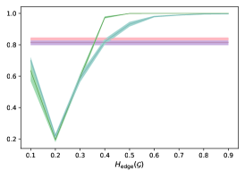
(a) RG: Model Curves

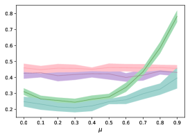
(b) PA: Model Curves

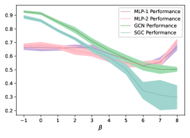
(c) GenCat: Model Curves

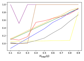
(d) RG: Metric Curves

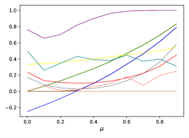
(e) PA: Metric Curves

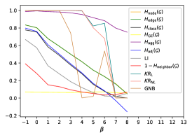
(f) GenCat: Metric Curves

Figure 1: Comparison of metrics on synthetic graphs with different generation methods. Note that $\text{H}_{\text{node}}$ overlaps with $\text{H}_{\text{edge}}$ in Figure (e) and (f). In Figure (e), $\text{H}_{\text{class}}(\mathcal{G})$ overlaps with $\text{H}_{\text{adj}}(\mathcal{G})$. $\text{KR}_{\text{L}}$, $\text{KR}_{\text{NL}}$ and GNB overlaps in Figure (d).

4.2 Evaluation of Metrics and Observation-Based Comparison

Evaluation of Metrics

The evaluation includes the following steps: 1) generate synthetic graphs with different homophily-related hyperparameters, e.g., edge homophily for regular graphs, $\mu$ for PA model and $\beta$ for GenCat; 2) for each generated graph, nodes are randomly splitted into train/validation/test sets, in proportion of 60%/20%/20%; 3) each baseline model (GCN, SGC-1, MLP-2 and MLP-1) is trained on every synthetic graph with the same hyperparameter searching range as [34], the mean test accuracy and standard deviation of $10$ runs are recorded; 4) calculate the corresponding metric values for each synthetic graph; 5) plot the metric curves and the performance curves of baseline models w.r.t. the homophily-related hyperparameters, compare their correlations.

Comparison and Observations

The performance curves of baseline models are shown in Figure 1 (a)(b)(c) and the metric curves are shown in Figure 1 (d)(e)(f). From the figures we observe that

• Inconsistent Shapes of GNN Performance Curves Between Methods. The curves in RG (Figure 1(a)) are fully U-shaped, which indicates the performance of GNNs in low-homophily area can rebound up to the same level as the high-homophily area. However, in PA and GenCat, the curves are partially U-shaped, which implies that the performance in heterophily area cannot rebound back to the same level as homophily area.

• Different Correlations Between Metrics and GNN Performance. The highest correlated metrics are inconsistent between figures. For example in Figure 1(d), the curves of $\text{KR}_{\text{L}},\text{KR}_{\text{NL}}$ and GNB highly correlate the curves of baseline GNNs on regular graphs. However, in PA, the curves of label informativeness and aggregated homophily have the highest correlations; and in GenCat, the curves of label informativeness and $\text{KR}_{\text{L}},\text{KR}_{\text{NL}}$ exhibit the strongest correlations.

Based on the above analysis, it is evident that getting a consistent and strict comparison results of the metrics based on observation is hard. Thus, we propose the first quantitative evaluation benchmarks for homophily metrics in the next subsection.

4.3 Fréchet Distance Based Quantitative Evaluation Benchmarks for Homophily Metrics

Table 4: Fréchet distance based quantitative comparison of homophily metrics on synthetic graphs

Metrics\Graphs	$\text{D}_{\text{Fr\'{e}chet}}$(Metric curve, GCN curve)				$\text{D}_{\text{Fr\'{e}chet}}$ (Metric curve, SGC-1 curve)
	RG	PA	GenCat	Ave Ranking	RG	PA	GenCat	Ave Ranking
$\text{H}_{\text{edge}}$	0.55	0.27	0.19	5.00	0.62	0.21	0.17	3.67
$\text{H}_{\text{node}}$	0.55	0.27	0.19	4.67	0.62	0.21	0.17	4.00
$\text{H}_{\text{class}}$	0.53	0.15	0.07	2.33	0.61	0.21	0.15	2.67
$\text{H}_{\text{adj}}$	0.55	0.27	0.19	4.33	0.62	0.21	0.17	3.33
$\text{H}_{\text{GE}}$	0.68	0.26	0.94	8.33	0.67	0.21	0.92	8.33
$\text{H}_{\text{agg}}$	0.50	0.42	0.51	6.33	0.48	0.40	0.46	5.33
LI	0.52	0.14	0.28	3.00	0.59	0.12	0.34	3.00
$\text{H}_{\text{neighbor}}$	0.51	0.26	0.50	4.33	0.58	0.18	0.50	4.00
GNB	0.55	0.38	0.48	6.67	0.62	0.48	0.50	7.33
$\text{KR}_{\text{L}}$	0.55	0.88	0.80	8.67	0.62	0.79	0.77	8.67
$\text{KR}_{\text{NL}}$	0.55	0.36	0.67	7.33	0.62	0.27	0.60	7.33

The Fréchet distance between two curves is a metric to measure the similarity between two arbitrary curves and it can be approximately calculated by the discrete Fréchet distance [64, 65]. A smaller distance value indicates higher similarity. In this section, we use the discrete Fréchet distance between the metric curves and GNN performance curves to evaluate and compare the homophily metrics quantitatively . The results are reported in Table 4 and a smaller value implies that the metric can better reflect GNN performance. From the results we can see that,

• Although some new proposed metrics can reveal the rebounding up phenomenon in extremely low homophily area, e.g., $\text{H}_{\text{agg}}$, the old homophily metrics, e.g.,$\text{H}_{\text{edge}},\text{H}_{\text{node}},\text{H}_{\text{class}}$, are still better at revealing GNN performance in most homophily area.

• On synthetic graphs with different generation methods, the metric can have different correlation with GNN performance. For example, curves of $\text{H}_{\text{GE}}$ have high correlation with GNN performance curves in PA generated graph, but have much lower correlation on GenCat generated graphs.

5 Conclusion

In this paper, we propose three pitfalls in the model and metric evaluation for heterophilic graph representation learning: 1) lacking hyperparameter tuning; 2) insufficient model evaluation on the real challenging heterophilic datasets; 3) absence of quantitative evaluation benchmark for homophily metrics on synthetic graphs. To address these issues, we fine-tune the baseline models to discover three different types of heterophilic graphs among $27$ most used benchmark datasets, i.e., malignant, benign and ambiguous heterophily datasets. We identify the real challenging tasks and reassess $10$ popular SOTA model with fine-tuned hyperparameters. At last, we design a Fréchet distance based quantitative evaluation benchmark for homophily metrics, and we compare $11$ popular metrics with our proposed benchmark.

Appendix A More Experimental Setups

A.1 Hyperparameter Searching Range

For every models and datasets, we perform a grid search for learning rate $\in\{{0.01,0.05,0.1}\}$, weight decay $\in\{0,5e-7,5e-6,1e-5,5e-5,1e-4,5e-4,1e-3,5e-3,1e-2\}$, dropout $\in\{0,0.1,0.3,0.5,0.7\}$ with the Adam optimizer. We use hidden unit $=128$ for wiki-cooc, 512 for roman-empire, amazon-ratings, minesweeper, tolokers, questions, Squirrel-filtered, Chameleon-filtered, and 64 for all the other datasets. These settings are used for GCN, SGC-1, MLP-2, MLP-1, and shared by other GNN models. Specific hyperparameters for are listed as follows

• GPRGNN: the weight is initialized by their Personalized PageRank, $\alpha\in\{0.1,0.2,0.5,0.9\}$ and $K=10$ power of the adjacency is used.

• BernNet: the propagation steps $K=10$.

• FAGCN: $\epsilon\in\{0.3,0.4,0.5\}$

• LINKX: the number of layers of $\text{MLP}_{\mathbf{A}}$ and $\text{MLP}_{\mathbf{X}}$ are in $\{1,2\}$.

• ACM-GCN: “structure_info" $\in\{0,1\}$, “variant" $\in\{0,1\}$, with “ACM-GCN+" and “ACM-GCN++".

• GBK-GNN: we set $\lambda=30$ and use the model based on GraphSage.

• FSGNN: 3-hop configuration under “all-feature" settings.

• APPNP: $\alpha\in\{0.1,0.2,0.5,0.9\}$ and $K=10$ power of the adjacency is used.

Appendix B Homophily Metrics

There are mainly four ways to define the metrics that describe the relations among node labels, features and graph structure to predict whether graph-aware models can outperform their coupled graph-agnostic counterparts.

Graph-Label Consistency

Four commonly used homophily metrics based on the consistency between node labels and graph structures are edge homophily [40, 24], node homophily [22], class homophily [29] and adjusted homophily [42] defined as follows:

$$\text{H}_{\text{edge}}(\mathcal{G})=\frac{\big{|}\{e_{uv}\mid e_{uv}\in\mathcal{E},y_{u}=y_{v}\}\big{|}}{|\mathcal{E}|};\text{H}_{\text{node}}(\mathcal{G})=\frac{1}{|\mathcal{V}|}\sum_{v\in\mathcal{V}}\frac{\big{|}\{u\mid u\in\mathcal{N}_{v},y_{u}=y_{v}\}\big{|}}{d_{v}};$$ (7)

$$\text{H}_{\text{class}}(\mathcal{G})\!=\!\frac{1}{C\!-\!1}\sum_{k=1}^{C}\bigg{[}h_{k}\!-\!\frac{\big{|}\{v\!\mid\!Y_{v,k}\!=\!1\}\big{|}}{N}\bigg{]}_{+},\text{ where }h_{k}\!=\!\frac{\sum_{v\in\mathcal{V},Y_{v,k}\!=\!1}\big{|}\{u\!\mid\!u\in\mathcal{N}_{v},y_{u}\!=\!y_{v}\}\big{|}}{\sum_{v\in\{v|Y_{v,k}=1\}}d_{v}};$$

$$\text{H}_{\text{adj}}(\mathcal{G})=\frac{\text{H}_{\text{edge}}-\sum_{c=1}^{C}\bar{p}_{c}^{2}}{1-\sum_{c=1}^{C}\bar{p}_{c}^{2}},\text{ where }\bar{p}_{c}=\frac{\sum_{v:y_{v}=c}d_{v}}{2|\mathcal{E}|}$$

where $\text{H}_{\text{node}}^{v}$ is the local homophily value for node $v$; $[a]_{+}=\max(a,0)$, $h_{k}$ is the class-wise homophily metric [29].

Note that $\text{H}_{\text{edge}}(\mathcal{G})$ measures the proportion of edges that connect two nodes in the same class; $\text{H}_{\text{node}}(\mathcal{G})$ evaluates the average proportion of edge-label consistency of all nodes; $\text{H}_{\text{class}}(\mathcal{G})$ tries to avoid sensitivity to imbalanced classes, which can make $\text{H}text{edge}(\mathcal{G})$ misleadingly large; $\text{H}_{\text{adj}}(\mathcal{G})$ is constructed to satisfy maximal agreement and constant baseline properties. The above definitions are all based on the linear feature-independent graph-label consistency. The inconsistency relation indicated by a small metric value implies that the graph structure has a negative effect on the performance of GNNs.

Similarity Based Metrics

Generalized edge homophily [43] and aggregation homophily [34] leverages similarity functions to define the metrics,

$$\leavevmode\resizebox{469.75499pt}{}{$\text{H}_{\text{GE}}(\mathcal{G})=\frac{\sum\limits_{(i,j)\in\mathcal{E}}\text{cos}(\bm{x}_{i},\bm{x}_{j})}{|\mathcal{E}|};\ \text{H}_{\text{agg}}(\mathcal{G})=\frac{1}{\left|\mathcal{V}\right|}\times\left|\left\{v\,\big{|}\,\mathrm{Mean}_{u}\big{(}\{S(\hat{{A}},Y)_{v,u}^{y_{u}=y_{v}}\}\big{)}\geq\mathrm{Mean}_{u}\big{(}\{S(\hat{{A}},Y)_{v,u}^{y_{u}\neq y_{v}}\}\big{)}\right\}\right|$}$$ (8)

where $\mathrm{Mean}_{u}\left(\{\cdot\}\right)$ takes the average over $u$ of a given multiset of values or variables and $S(\hat{{A}},Y)=\hat{{A}}Y(\hat{{A}}Y)^{\top}$ is the post-aggregation node similarity matrix. These two metrics are feature-dependent.

$\text{H}_{\text{GE}}(\mathcal{G})$ generalizes $\text{H}_{\text{edge}}(\mathcal{G})$ to the the cosine similarities between node features; $\text{H}_{\text{agg}}(\mathcal{G})$ measures the proportion of nodes $v\in\mathcal{V}$ as which the average $S(\hat{{A}},Y)$ weights on the set of nodes in the same class (including $v$) is larger than that in other classes. They are both feature-dependent metrics.

Neighborhood Identifiability/Informativeness

Label informativeness  [42] and neighborhood identifiability [44] leverage the neighborhood distribution instead of pairwise comparison to define the metrics,

$$\leavevmode\resizebox{469.75499pt}{}{$\text{LI}=-\frac{\sum_{c_{1},c_{2}}p_{c_{1},c_{2}}\log\frac{p_{c_{1},c_{2}}}{\bar{p}_{c_{1}}\bar{p}_{c_{2}}}}{\sum_{c}\bar{p}_{c}\log\bar{p}_{c}};\ {H}_{\text{neighbor }}(\mathcal{G})=\sum_{k=1}^{C}\frac{n_{k}}{N}\text{H}_{\text{neighbor }}^{k},\text{ where }{H}_{\text{neighbor }}^{k}=\frac{-\sum_{i=1}^{C}\tilde{\sigma}_{i}^{k}\log\left(\tilde{\sigma}_{i}^{k}\right)}{\log(C)}.$}$$ (9)

where $p_{c_{1},c_{2}}=\sum_{(u,v)\in\mathcal{E}}\frac{\bm{1}\left\{y_{u}=c_{1},y_{v}=c_{2}\right\}}{2|\mathcal{E}|},c_{1},c_{2}\in\{1,\dots,C\}$; $A^{k}\in\mathbb{R}^{n_{k}\times C}$ is a class-level neighborhood label distribution matrix for each class $k$, where $k=1,\ldots,C$ for different classes and $n_{k}$ indicates the number of nodes with the label $k$, $(A^{k})_{i,c}$ is the proportion of the neighbors of node $i$ belonging to class $c$, $\sigma_{1}^{k},\sigma_{2}^{k},\ldots,\sigma_{C}^{k}$ denote singular values of $A^{k}$, they are normalized to $\sum_{c=1}^{C}\tilde{\sigma}_{c}^{k}=1$, $c=1,\ldots,C$ is the index of singular values.

LI is to characterize different connectivity patterns by measuring the informativeness of the label of a neighbor for the label of a node; $\text{H}_{\text{neighbor}}(\mathcal{G})$ is a weighted sum of ${H}_{\text{neighbor}}(\mathcal{G})$, quantifying neighborhood identifiability through the entropy of the singular value distribution of $A^{k}$, which is a generalization of the von Neumann entropy in quantum statistical mechanics [67] that measures the pureness/information of a quantum-mechanical system. This metric effectively measures the complexity/randomness of neighborhood distributions by indicating the number of vectors (or neighbor patterns) necessary to sufficiently describe the neighborhood label distribution matrix.

Hypothesis Testing Based Performance Metrics

Luan et al. [39] proposed classifier-based performance metric (CPM), which uses the p-value of hypothesis testing as the metric to measure the node distinguishability of the aggregated features compared with the original features.

They first randomly sample 500 labeled nodes from $\mathcal{V}$ and splits them into 60%/40% as "training" and "test" data. The original features $X$ and aggregated features $H$ of the sampled training and test nodes can be calculated and are then fed into a given classifier. The prediction accuracy on the test nodes will be computed directly with the feedforward method. This process will be repeated 100 times to get 100 samples of prediction accuracy for $X$ and $H=\hat{A}X$. Then, for the given classifier, they compute the p-value of the following hypothesis testing,

$$\leavevmode\resizebox{469.75499pt}{}{$\text{H}_{0}:\text{Acc}(\text{Classifier}(H))\geq\text{Acc}(\text{Classifier}(X));\ \text{H}_{1}:\text{Acc}(\text{Classifier}(H))<\text{Acc}(\text{Classifier}(X))$}$$ (10)

The p-value can provide a statistical threshold value, such as 0.05, to indicate whether $H$ is significantly better than $X$ for node classification. To capture the feature-based linear or non-linear information efficiently, Luan et al.choose Gaussian Naïve Bayes (GNB) [45] and Kernel Regression (KR) with Neural Network Gaussian Process (NNGP) [46, 47, 48, 49] as the classifiers, which do not require iterative training.

Overall, $\text{H}_{\text{adj}}$ can assume negative values, while other metrics all fall within the range of $[0,1]$. Except for $\text{H}_{\text{neighbor}}(\mathcal{G})$, where a smaller value indicates more identifiable, the other metrics with a value closer to $1$ indicate strong homophily and suggest that the connected nodes tend to share the same label, implying that graph-aware models are more likely to outperform their coupled graph-agnostic model, and vice versa.

$\text{H}_{\text{edge}},\text{H}_{\text{node}},\text{H}_{\text{class}},\text{H}_{\text{adj}}$ and LI are linear feature-independent metrics. $LI$ and ${H}_{\text{neighbor}}(\mathcal{G})$ are nonlinear feature-independent metrics. $\text{H}_{\text{GE}}$ and $\text{H}_{\text{agg}}$ are feature-dependent and measure the linear similarity between nodes. CPM is the first metric that can capture nonlinear feature-dependent information and provide accurate threshold values to indicate the superiority of graph-aware models. In Section 4, we will introduce the approach for the comparison of the above metrics by synthetic graphs with different generation methods.

References

- Sperduti [1993] Alessandro Sperduti. Encoding labeled graphs by labeling raam. Advances in Neural Information Processing Systems, 6, 1993.
- Goller and Kuchler [1996] Christoph Goller and Andreas Kuchler. Learning task-dependent distributed representations by backpropagation through structure. In Proceedings of International Conference on Neural Networks (ICNN’96), volume 1, pages 347–352. IEEE, 1996.
- Sperduti and Starita [1997] Alessandro Sperduti and Antonina Starita. Supervised neural networks for the classification of structures. IEEE Transactions on Neural Networks, 8(3):714–735, 1997.
- Frasconi et al. [1998] Paolo Frasconi, Marco Gori, and Alessandro Sperduti. A general framework for adaptive processing of data structures. IEEE transactions on Neural Networks, 9(5):768–786, 1998.
- Scarselli et al. [2008] Franco Scarselli, Marco Gori, Ah Chung Tsoi, Markus Hagenbuchner, and Gabriele Monfardini. The graph neural network model. IEEE transactions on neural networks, 20(1):61–80, 2008.
- Bruna et al. [2014] Joan Bruna, Wojciech Zaremba, Arthur Szlam, and Yann LeCun. Spectral networks and deep locally connected networks on graphs. In 2nd International Conference on Learning Representations, ICLR 2014, 2014.
- Defferrard et al. [2016] Michaël Defferrard, Xavier Bresson, and Pierre Vandergheynst. Convolutional neural networks on graphs with fast localized spectral filtering. Advances in neural information processing systems, 29, 2016.
- Kipf and Welling [2016] Thomas N Kipf and Max Welling. Semi-supervised classification with graph convolutional networks. In International Conference on Learning Representations, 2016.
- Hamilton et al. [2017] Will Hamilton, Zhitao Ying, and Jure Leskovec. Inductive representation learning on large graphs. Advances in neural information processing systems, 30, 2017.
- Gilmer et al. [2017] Justin Gilmer, Samuel S Schoenholz, Patrick F Riley, Oriol Vinyals, and George E Dahl. Neural message passing for quantum chemistry. In Proceedings of the 34th International Conference on Machine Learning-Volume 70, pages 1263–1272. JMLR. org, 2017.
- Velickovic et al. [2018] Petar Velickovic, Guillem Cucurull, Arantxa Casanova, Adriana Romero, Pietro Liò, and Yoshua Bengio. Graph attention networks. In International Conference on Learning Representations, 2018.
- Xu et al. [2018] Keyulu Xu, Weihua Hu, Jure Leskovec, and Stefanie Jegelka. How powerful are graph neural networks? In International Conference on Learning Representations, 2018.
- Luan et al. [2019] Sitao Luan, Mingde Zhao, Xiao-Wen Chang, and Doina Precup. Break the ceiling: Stronger multi-scale deep graph convolutional networks. Advances in neural information processing systems, 32, 2019.
- Monti et al. [2017] Federico Monti, Davide Boscaini, Jonathan Masci, Emanuele Rodola, Jan Svoboda, and Michael M Bronstein. Geometric deep learning on graphs and manifolds using mixture model cnns. In Proceedings of the IEEE Conference on Computer Vision and Pattern Recognition, pages 5115–5124, 2017.
- Ying et al. [2018] Rex Ying, Ruining He, Kaifeng Chen, Pong Eksombatchai, William L Hamilton, and Jure Leskovec. Graph convolutional neural networks for web-scale recommender systems. In Proceedings of the 24th ACM SIGKDD international conference on knowledge discovery & data mining, pages 974–983, 2018.
- Pfaff et al. [2020] Tobias Pfaff, Meire Fortunato, Alvaro Sanchez-Gonzalez, and Peter Battaglia. Learning mesh-based simulation with graph networks. In International Conference on Learning Representations, 2020.
- Zhao et al. [2021] Mingde Zhao, Zhen Liu, Sitao Luan, Shuyuan Zhang, Doina Precup, and Yoshua Bengio. A consciousness-inspired planning agent for model-based reinforcement learning. Advances in neural information processing systems, 34:1569–1581, 2021.
- Bongini et al. [2021] Pietro Bongini, Monica Bianchini, and Franco Scarselli. Molecular generative graph neural networks for drug discovery. Neurocomputing, 450:242–252, 2021.
- Hua et al. [2024] Chenqing Hua, Sitao Luan, Minkai Xu, Zhitao Ying, Jie Fu, Stefano Ermon, and Doina Precup. Mudiff: Unified diffusion for complete molecule generation. In Learning on Graphs Conference, pages 33–1. PMLR, 2024.
- Lu et al. [2024a] Qincheng Lu, Sitao Luan, and Xiao-Wen Chang. Gcepnet: Graph convolution-enhanced expectation propagation for massive mimo detection. arXiv preprint arXiv:2404.14886, 2024a.
- McPherson et al. [2001] Miller McPherson, Lynn Smith-Lovin, and James M Cook. Birds of a feather: Homophily in social networks. Annual review of sociology, 27(1):415–444, 2001.
- Pei et al. [2020] Hongbin Pei, Bingzhe Wei, Kevin Chen-Chuan Chang, Yu Lei, and Bo Yang. Geom-gcn: Geometric graph convolutional networks. In International Conference on Learning Representations, 2020.
- Hamilton [2020] William L Hamilton. Graph representation learning. Synthesis Lectures on Artifical Intelligence and Machine Learning, 14(3):1–159, 2020.
- Zhu et al. [2020] Jiong Zhu, Yujun Yan, Lingxiao Zhao, Mark Heimann, Leman Akoglu, and Danai Koutra. Beyond homophily in graph neural networks: Current limitations and effective designs. Advances in Neural Information Processing Systems, 33, 2020.
- Lozares et al. [2014] Carlos Lozares, Joan Miquel Verd, Irene Cruz, and Oriol Barranco. Homophily and heterophily in personal networks. from mutual acquaintance to relationship intensity. Quality & Quantity, 48:2657–2670, 2014.
- Luan et al. [2024a] Sitao Luan, Chenqing Hua, Qincheng Lu, Liheng Ma, Lirong Wu, Xinyu Wang, Minkai Xu, Xiao-Wen Chang, Doina Precup, Rex Ying, et al. The heterophilic graph learning handbook: Benchmarks, models, theoretical analysis, applications and challenges. arXiv preprint arXiv:2407.09618, 2024a.
- Luan et al. [2022a] Sitao Luan, Mingde Zhao, Chenqing Hua, Xiao-Wen Chang, and Doina Precup. Complete the missing half: Augmenting aggregation filtering with diversification for graph convolutional networks. In NeurIPS 2022 Workshop: New Frontiers in Graph Learning, 2022a.
- Bo et al. [2021] Deyu Bo, Xiao Wang, Chuan Shi, and Huawei Shen. Beyond low-frequency information in graph convolutional networks. In Proceedings of the AAAI Conference on Artificial Intelligence, volume 35, pages 3950–3957, 2021.
- Lim et al. [2021a] Derek Lim, Xiuyu Li, Felix Hohne, and Ser-Nam Lim. New benchmarks for learning on non-homophilous graphs. arXiv preprint arXiv:2104.01404, 2021a.
- Chien et al. [2021] Eli Chien, Jianhao Peng, Pan Li, and Olgica Milenkovic. Adaptive universal generalized pagerank graph neural network. In International Conference on Learning Representations, 2021.
- Yan et al. [2022] Yujun Yan, Milad Hashemi, Kevin Swersky, Yaoqing Yang, and Danai Koutra. Two sides of the same coin: Heterophily and oversmoothing in graph convolutional neural networks. In 2022 IEEE International Conference on Data Mining (ICDM), pages 1287–1292. IEEE, 2022.
- He et al. [2021] Mingguo He, Zhewei Wei, Hongteng Xu, et al. Bernnet: Learning arbitrary graph spectral filters via bernstein approximation. Advances in Neural Information Processing Systems, 34, 2021.
- Li et al. [2022] Xiang Li, Renyu Zhu, Yao Cheng, Caihua Shan, Siqiang Luo, Dongsheng Li, and Weining Qian. Finding global homophily in graph neural networks when meeting heterophily. In International Conference on Machine Learning, pages 13242–13256. PMLR, 2022.
- Luan et al. [2022b] Sitao Luan, Chenqing Hua, Qincheng Lu, Jiaqi Zhu, Mingde Zhao, Shuyuan Zhang, Xiao-Wen Chang, and Doina Precup. Revisiting heterophily for graph neural networks. Advances in neural information processing systems, 35:1362–1375, 2022b.
- Lu et al. [2024b] Qincheng Lu, Jiaqi Zhu, Sitao Luan, and Xiao-Wen Chang. Representation learning on heterophilic graph with directional neighborhood attention. arXiv preprint arXiv:2403.01475, 2024b.
- Zheng et al. [2024] Yilun Zheng, Sitao Luan, and Lihui Chen. What is missing in homophily? disentangling graph homophily for graph neural networks. arXiv preprint arXiv:2406.18854, 2024.
- Ma et al. [2021] Yao Ma, Xiaorui Liu, Neil Shah, and Jiliang Tang. Is homophily a necessity for graph neural networks? In International Conference on Learning Representations, 2021.
- Luan et al. [2021] Sitao Luan, Chenqing Hua, Qincheng Lu, Jiaqi Zhu, Mingde Zhao, Shuyuan Zhang, Xiao-Wen Chang, and Doina Precup. Is heterophily a real nightmare for graph neural networks to do node classification? arXiv preprint arXiv:2109.05641, 2021.
- Luan et al. [2024b] Sitao Luan, Chenqing Hua, Minkai Xu, Qincheng Lu, Jiaqi Zhu, Xiao-Wen Chang, Jie Fu, Jure Leskovec, and Doina Precup. When do graph neural networks help with node classification? investigating the homophily principle on node distinguishability. Advances in Neural Information Processing Systems, 36, 2024b.
- Abu-El-Haija et al. [2019] Sami Abu-El-Haija, Bryan Perozzi, Amol Kapoor, Nazanin Alipourfard, Kristina Lerman, Hrayr Harutyunyan, Greg Ver Steeg, and Aram Galstyan. Mixhop: Higher-order graph convolutional architectures via sparsified neighborhood mixing. In international conference on machine learning, pages 21–29. PMLR, 2019.
- Wu et al. [2019] Felix Wu, Amauri Souza, Tianyi Zhang, Christopher Fifty, Tao Yu, and Kilian Weinberger. Simplifying graph convolutional networks. In International conference on machine learning, pages 6861–6871. PMLR, 2019.
- Platonov et al. [2023] Oleg Platonov, Denis Kuznedelev, Artem Babenko, and Liudmila Prokhorenkova. Characterizing graph datasets for node classification: Beyond homophily-heterophily dichotomy. Advances in Neural Information Processing Systems, 36, 2023.
- Jin et al. [2022] Di Jin, Rui Wang, Meng Ge, Dongxiao He, Xiang Li, Wei Lin, and Weixiong Zhang. Raw-gnn: Random walk aggregation based graph neural network. In 31st International Joint Conference on Artificial Intelligence, IJCAI 2022, pages 2108–2114. International Joint Conferences on Artificial Intelligence, 2022.
- Chen et al. [2023] Jie Chen, Shouzhen Chen, Junbin Gao, Zengfeng Huang, Junping Zhang, and Jian Pu. Exploiting neighbor effect: Conv-agnostic gnn framework for graphs with heterophily. IEEE Transactions on Neural Networks and Learning Systems, 2023.
- Hastie et al. [2009] Trevor Hastie, Robert Tibshirani, Jerome H Friedman, and Jerome H Friedman. The elements of statistical learning: data mining, inference, and prediction, volume 2. Springer, 2009.
- Lee et al. [2018] Jaehoon Lee, Yasaman Bahri, Roman Novak, Samuel S Schoenholz, Jeffrey Pennington, and Jascha Sohl-Dickstein. Deep neural networks as gaussian processes. In International Conference on Learning Representations, 2018.
- Arora et al. [2019] Sanjeev Arora, Simon S Du, Wei Hu, Zhiyuan Li, Russ R Salakhutdinov, and Ruosong Wang. On exact computation with an infinitely wide neural net. Advances in neural information processing systems, 32, 2019.
- Garriga-Alonso et al. [2018] Adrià Garriga-Alonso, Carl Edward Rasmussen, and Laurence Aitchison. Deep convolutional networks as shallow gaussian processes. In International Conference on Learning Representations, 2018.
- Matthews et al. [2018] Alexander G de G Matthews, Mark Rowland, Jiri Hron, Richard E Turner, and Zoubin Ghahramani. Gaussian process behaviour in wide deep neural networks. In International Conference on Learning Representations, 2018.
- Rozemberczki et al. [2021] Benedek Rozemberczki, Carl Allen, and Rik Sarkar. Multi-scale attributed node embedding. Journal of Complex Networks, 9(2):cnab014, 2021.
- Lim et al. [2021b] Derek Lim, Felix Hohne, Xiuyu Li, Sijia Linda Huang, Vaishnavi Gupta, Omkar Bhalerao, and Ser Nam Lim. Large scale learning on non-homophilous graphs: New benchmarks and strong simple methods. Advances in Neural Information Processing Systems, 34:20887–20902, 2021b.
- Sun et al. [2022] Yifei Sun, Haoran Deng, Yang Yang, Chunping Wang, Jiarong Xu, Renhong Huang, Linfeng Cao, Yang Wang, and Lei Chen. Beyond homophily: structure-aware path aggregation graph neural network. In Proceedings of the Thirty-First International Joint Conference on Artificial Intelligence, IJCAI, pages 2233–2240, 2022.
- Platonov et al. [2022] Oleg Platonov, Denis Kuznedelev, Michael Diskin, Artem Babenko, and Liudmila Prokhorenkova. A critical look at the evaluation of gnns under heterophily: Are we really making progress? In The Eleventh International Conference on Learning Representations, 2022.
- Zhou et al. [2024] Zhiyao Zhou, Sheng Zhou, Bochao Mao, Xuanyi Zhou, Jiawei Chen, Qiaoyu Tan, Daochen Zha, Yan Feng, Chun Chen, and Can Wang. Opengsl: A comprehensive benchmark for graph structure learning. Advances in Neural Information Processing Systems, 36, 2024.
- Yang et al. [2016] Zhilin Yang, William Cohen, and Ruslan Salakhudinov. Revisiting semi-supervised learning with graph embeddings. In International conference on machine learning, pages 40–48. PMLR, 2016.
- Fey and Lenssen [2019] Matthias Fey and Jan Eric Lenssen. Fast graph representation learning with pytorch geometric. arXiv preprint arXiv:1903.02428, 2019.
- Du et al. [2022] Lun Du, Xiaozhou Shi, Qiang Fu, Xiaojun Ma, Hengyu Liu, Shi Han, and Dongmei Zhang. Gbk-gnn: Gated bi-kernel graph neural networks for modeling both homophily and heterophily. In Proceedings of the ACM Web Conference 2022, pages 1550–1558, 2022.
- Maurya et al. [2022] Sunil Kumar Maurya, Xin Liu, and Tsuyoshi Murata. Simplifying approach to node classification in graph neural networks. Journal of Computational Science, 62:101695, 2022.
- Gasteiger et al. [2018] Johannes Gasteiger, Aleksandar Bojchevski, and Stephan Günnemann. Predict then propagate: Graph neural networks meet personalized pagerank. In International Conference on Learning Representations, 2018.
- Barabási and Albert [1999] Albert-László Barabási and Réka Albert. Emergence of scaling in random networks. science, 286(5439):509–512, 1999.
- Karimi et al. [2018] Fariba Karimi, Mathieu Génois, Claudia Wagner, Philipp Singer, and Markus Strohmaier. Homophily influences ranking of minorities in social networks. Scientific reports, 8(1):11077, 2018.
- Maekawa et al. [2022] Seiji Maekawa, Koki Noda, Yuya Sasaki, et al. Beyond real-world benchmark datasets: An empirical study of node classification with gnns. Advances in Neural Information Processing Systems, 35:5562–5574, 2022.
- Maekawa et al. [2023] Seiji Maekawa, Yuya Sasaki, George Fletcher, and Makoto Onizuka. Gencat: Generating attributed graphs with controlled relationships between classes, attributes, and topology. Information Systems, 115:102195, 2023.
- Alt and Godau [1995] Helmut Alt and Michael Godau. Computing the fréchet distance between two polygonal curves. International Journal of Computational Geometry & Applications, 5(01n02):75–91, 1995.
- Efrat et al. [2002] Efrat, Guibas, Sariel Har-Peled, and Murali. New similarity measures between polylines with applications to morphing and polygon sweeping. Discrete & Computational Geometry, 28:535–569, 2002.
- Eiter and Mannila [1994] Thomas Eiter and Heikki Mannila. Computing discrete fréchet distance. 1994.
- Bengtsson and Życzkowski [2017] Ingemar Bengtsson and Karol Życzkowski. Geometry of quantum states: an introduction to quantum entanglement. Cambridge university press, 2017.
- Luan et al. [2023] Sitao Luan, Chenqing Hua, Qincheng Lu, Jiaqi Zhu, Xiao-Wen Chang, and Doina Precup. When do we need graph neural networks for node classification? In International Conference on Complex Networks and Their Applications, pages 37–48. Springer, 2023.