Examining the Relationship Between the Persistent Emission and the Accretion Rate During a Type I X-ray Burst

Abstract

The accretion flow onto a neutron star will be impacted due to irradiation by a Type I X-ray burst. The burst radiation exerts Poynting-Robertson (PR) drag on the accretion disk, leading to an enhanced mass accretion rate. Observations of X-ray bursts often find evidence that the normalization of the disk-generated persistent emission (commonly denoted by the factor $f_{a}$) increases during a burst, and changes in $f_{a}$ have been used to infer the evolution in the mass accretion rate due to PR drag. Here, we examine this proposed relationship between $f_{a}$ and mass accretion rate enhancement using time-resolved data from simulations of accretion disks impacted by Type I X-ray bursts. We consider bursts from both spinning and non-spinning neutron stars and track both the change in accretion rate due to PR grad and the disk emission spectra during the burst. Regardless of the neutron star spin, we find that $f_{a}$ strongly correlates with the disk temperature and only weakly follows the mass accretion rate (the Pearson correlation coefficients are $\leq 0.63$ in the latter case). Additionally, heating causes the disk to emit at higher energies, reducing its contribution to a soft excess. We conclude that $f_{a}$ cannot accurately capture the mass accretion rate enhancement and is rather a tracer of the disk temperature.

1 Introduction

Neutron stars in low-mass X-ray binaries accrete matter from their companion star via Roche-Lobe overflow. The accreted matter moves inwards through an accretion disk aided by viscous processes moving angular momentum outwards (for a review, see Abramowicz & Fragile, 2013). The accretion liberates potential energy, a large fraction of which is radiated by the disk. If the accretion disk is optically thick, its spectrum is expected to be consistent with a multicolor blackbody, where the blackbody temperature varies with radius (e.g., Mitsuda et al., 1984; Kubota et al., 2005).

The accretion disk around neutron stars in these systems can be impacted by Type I X-ray bursts (for a review of Type I X-ray bursts, see Galloway & Keek, 2021). Type I X-ray bursts occur due to the ongoing accumulation of accreted material onto the neutron star surface. The accumulation of matter gradually increases the temperature and pressure at the neutron star surface, which can cause unstable nuclear burning. This unstable burning consumes the accumulated matter and heats the neutron star. The resulting X-ray burst radiates $\sim 10^{39}$ ergs away over a time span usually lasting on the order of tens of seconds (e.g., Bult et al., 2019; Galloway et al., 2020; Güver et al., 2022a; Yan et al., 2024).

The burst radiation illuminates the neutron star environment, leading to structural and spectral changes of the accretion flow (for a review, see Degenaar et al., 2018). A common observation is a drop in hard X-ray emission during bursts (e.g. Maccarone & Coppi, 2003; Ji et al., 2014; Sánchez-Fernández et al., 2020; Peng et al., 2024), which has been connected to the cooling of the corona, a region containing hot electrons (e.g., Fragile et al., 2018a; Speicher et al., 2020). Reprocessed emission from the accretion disk produces a reflection spectrum. During X-ray bursts, reflection is observable, for instance, through the detection of emission lines (e.g., Ballantyne & Strohmayer, 2004; Degenaar et al., 2013; Keek et al., 2017; Bult et al., 2019), which will evolve during bursts (Speicher et al., 2022).

Furthermore, observations suggest that the burst enhances the accretion flow emission. Worpel et al. (2013) and Worpel et al. (2015) introduced a normalization factor $f_{a}$ for the accretion-powered preburst emission, also called the persistent emission, and showed that $f_{a}>1$ during most bursts. Since its introduction, $f_{a}$ has become a common tool in burst analysis due to its ability to improve spectral fits (Jaisawal et al., 2019; Bult et al., 2022; Yu et al., 2024; Lu et al., 2024), and also by being able to account for a soft excess below 3 keV (e.g., Keek et al., 2018; Chen et al., 2022; Güver et al., 2022a).

The increase in the persistent emission during the burst has been attributed to Poynting-Robertson (PR) drag (Robertson, 1937). Burst photons exert PR drag onto the disk material, removing angular momentum. The angular momentum loss expedites the material infall and thus increases the mass accretion rate, which raises the accretion luminosity and its emission (Walker & Meszaros, 1989; Walker, 1992). Simulations of accretion flows impacted by X-ray bursts showed that PR drag can enhance the mass accretion rate by over an order of magnitude (Fragile et al., 2018a, 2020; Speicher et al., 2023), similar to the increase in $f_{a}$ inferred from burst observations (e.g., Worpel et al., 2015; Bult et al., 2022).

However, how the mass accretion rate enhancement translates into $f_{a}$ is not understood. While in the thin disk simulations by Fragile et al. (2020) and Speicher et al. (2023) the mass accretion rate significantly increased during the burst, the burst irradiation also heated the accretion disk. The increase in temperature at the accretion disk surface will modify its spectrum, and the heating effect could be mistaken as the impact of an enhanced mass accretion rate. Likewise, while $f_{a}$ can be used to fit the soft excess, this feature can also be explained with reflection (e.g. Bult et al., 2019; Speicher et al., 2022; Zhao et al., 2022).

This paper examines the relationship between the normalization factor $f_{a}$ and the mass accretion rate enhancement using the simulation data by Speicher et al. (2023). In addition, we will investigate the suitability of $f_{a}$ to account for the soft excess. In Section 2, we outline our calculations, with results presented in Section 3. We discuss the results in Section 4 and conclude with Section 5.

2 Methods

2.1 Calculation of the disk emission

We calculate the emission of the accretion disk using data from the four Cosmos++ (e.g., Anninos et al., 2005; Fragile et al., 2012, 2014) simulations analyzed by Speicher et al. (2023). The simulation space covers a radial range of 10.7 km $\lesssim r\lesssim$350 km and a polar angular range of $0\lesssim\theta\lesssim\pi$. The space is subdivided into cells, with more being concentrated towards the equatorial plane and smaller radii. Each simulation consists of a neutron star within the inner simulation boundary and an accretion disk within the simulation space. The neutron star has a mass of $M=1.45$ M_⊙ and radius $R=10.7$ km. In two simulations, the neutron star does not spin ($a_{*}=0$), while in the other two simulations, $a_{*}=0.2$ and the rotational frequency is 500 Hz. The spin parameter $a_{*}$ is calculated as $a_{*}=cJ/GM^{2}$, where $J$ is the angular momentum (for further details, see Speicher et al., 2023).

The accretion disks are initialized following the gas-pressure-dominated regime of the $\alpha$ model (Shakura & Sunyaev, 1973), with the viscosity parameter $\alpha=0.025$. Initially, the disks are in hydrostatic and thermal equilibrium. We assume that all magnetic fields are weak enough to be negligible.

In each simulation set, the neutron star is either quiescent or emits burst radiation isotropically as observed in the neutron star’s rest frame. The luminosity $L$ of the simulated bursts (black solid line in Fig.1) follows the lightcurve (e.g., Norris et al., 2005; Barrière et al., 2015),

$$L(t)=L_{0}e^{2\left(\tau_{1}/\tau_{2}\right)^{1/2}}e^{-\frac{\tau_{1}}{t-t_{s}}-\frac{t-t_{\mathrm{s}}}{\tau_{2}}},$$ (1)

where $L_{0}=10^{38}$ erg s^-1, $t_{\mathrm{s}}=-0.25$ s, $\tau_{1}=6$ s, and $\tau_{2}=1$ s. Within the simulation space, Cosmos++ solves for the interaction between the burst radiation and the gas of the disk by evolving general relativistic, radiative, viscous hydrodynamics equations (e.g., Fragile et al., 2018b).

We time-average gas-temperature and mass density data from the simulation within several $\approx 0.4$ s long time intervals (Fig. 1, shaded areas) with each time interval separated by $\approx 7\times 10^{-3}$ s. The burst simulations ran for $\approx 4.1$ s, yielding nine time intervals labeled A through I. The no-burst simulations ran for $\approx 3.2$ s, but because disk properties vary negligibly in this setup we analyze data from their time-interval F.

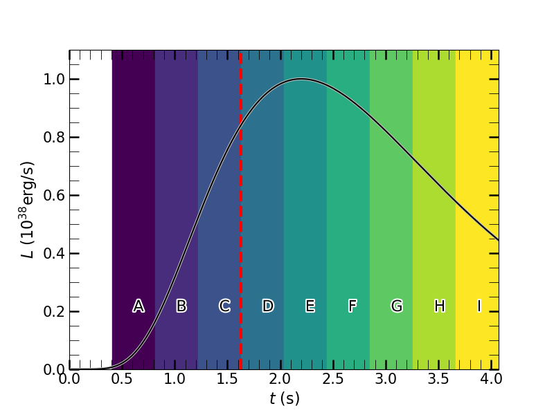
Figure 1: Luminosity profile (eq. 1) of the burst in the simulations by Speicher et al. (2023). The luminosity (black solid line) peaks at $10^{38}$ erg s^-1 at $\approx 2.2$ s. The shaded regions mark $\approx 0.4$s long time intervals, during which we time-average the simulation data to calculate the disk emission (eq. 2). Due to a transient numerical event, we only analyze the time intervals past the red dashed line for the $a_{*}=0.2$ burst simulation. For all no-burst simulations we use time interval F to calculate disk properties.

During each time interval, we assume that the disk radiates as a multicolor blackbody. Its emission is evaluated between an inner radius $r_{in}$ and an outer radius $r_{out}$, (e.g., Zdziarski et al., 2022),

$$\nu L_{\nu}=\frac{4\pi h\nu^{4}}{c^{2}}\\ \int_{r_{in}}^{r_{out}}\frac{r\,ds}{f_{c}\left[T_{eff}\right]^{4}\left\{\exp\left[h\nu/kf_{c}T_{eff}\right]-1\right\}},$$ (2)

where $h$ is Planck’s constant, $c$ the speed of light and $T_{eff}$ the effective temperature. As the disk is not flat and changes shape during the simulations with bursts the incremental length $ds=\sqrt{1+\left(\frac{dz}{dr}\right)^{2}}dr$. We fix $dr=10$ m and interpolate the simulation data to find $r$ and $z$ for use in Eq. 2.

The inner radius $r_{in}$ corresponds to the time-averaged radial position where the density-weighted surface density is the closest to 250 g cm^-2, following the definition of Speicher et al. (2023). In the $a_{*}=0$ burst simulations, $r_{in}$ moves outwards from $\approx 12.9$ km in time interval A to $\approx 14.4$ km in interval I due to PR drag. In the $a_{*}=0.2$ burst simulations, $r_{in}\approx 13$ km in time interval D and reaches $\approx 13.5$ km in interval I. In the no-burst simulations, $r_{in}$ is $\approx 12.9$ km ($a_{*}=0$) and $\approx 11.5$ km ($a_{*}=0.2$), both close to the respective radii of the innermost stable circular orbits $r_{\mathrm{isco}}$ of $12.85$ km ($a_{*}=0$) and $11.41$ km ($a_{*}=0.2$). The outer radius $r_{out}$ is set to 300 km, close to the outer simulation boundary but not so close as to introduce boundary effects.

The emitted spectrum will differ from a blackbody due to scattering processes. These deviations are captured with a color correction factor $f_{c}$, (Done et al., 2012),

$$f_{c}\left(T_{eff}\right)=\left(\frac{72\,\mathrm{keV}}{kT_{eff}}\right)^{1/9}.$$ (3)

In our calculations, $f_{c}$ varies between $\approx 1.5$ and $\approx 2.2$, consistent with previous results (e.g., Kubota et al., 2010; Suleimanov et al., 2012). Color corrections $>1$ will reduce and shift the emission to higher energies.

With the assumption that the accretion disk radiates as a color-corrected blackbody at every radius, we equate $T_{eff}$ to the gas temperature where $\tau$ is first $\geq 1$, with $\tau$ being the optical depth due to Thomson scattering integrated towards the equatorial plane. Examples of radial temperature profiles for time intervals A (blue solid line), E (red dotted line) and I (green dash-dotted line) are shown in Fig. 2 for the $a_{*}=0$ burst simulation. For visualization, the plotted temperature profiles have been smoothed by calculating the moving average with varying window sizes. Due to the strong illumination by the X-ray burst, the disk temperature is higher during the burst than in interval F of the no-burst simulation (black dashed line). The disk remains hot in the burst tail, visible by the little difference in temperature profiles of intervals I and E. The disk temperatures are also spin dependent, with the simulated $a_{*}=0.2$ disk being hotter than the $a_{*}=0$ disk (see also Speicher et al., 2023). We again use linear interpolation of the simulation data and $dr=10$ m to find the $T_{eff}$ values for use in Eqs. 2 and 3.

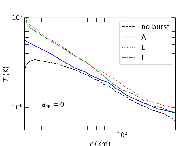
Figure 2: Radial temperature profile of the $a_{*}=0$ burst simulations for intervals A (blue solid line), E (red dotted line), and F (green dash-dotted line). The temperature profile of the no-burst simulation (black dashed line) is from interval F. The temperatures are located where the optical depth due to Thomson scattering, integrated towards the equatorial plane, first surpasses 1 and are equated to $T_{eff}$ for eq. 2 and 3. The plotted temperature profiles have been smoothed for visualization by calculating moving averages with varying window sizes.

With our interpolated values, we numerically integrate eq. 2 using the trapezoidal method for a linearly spaced, 600-entry-long energy grid between $\approx 8\times 10^{-3}$ keV and $\approx 33$ keV. For the $a_{*}=0$ burst simulation, we calculate spectra for all time intervals A-I. The $a_{*}=0.2$ burst simulation experienced a transient numerical event at $\lesssim 1$ s (see also Speicher et al., 2023), so we only calculate spectra for intervals D-I (those past the red dashed line in Fig. 1). We compare each spectrum from the burst simulations with the spectra of the corresponding no-burst simulations at their time interval F.

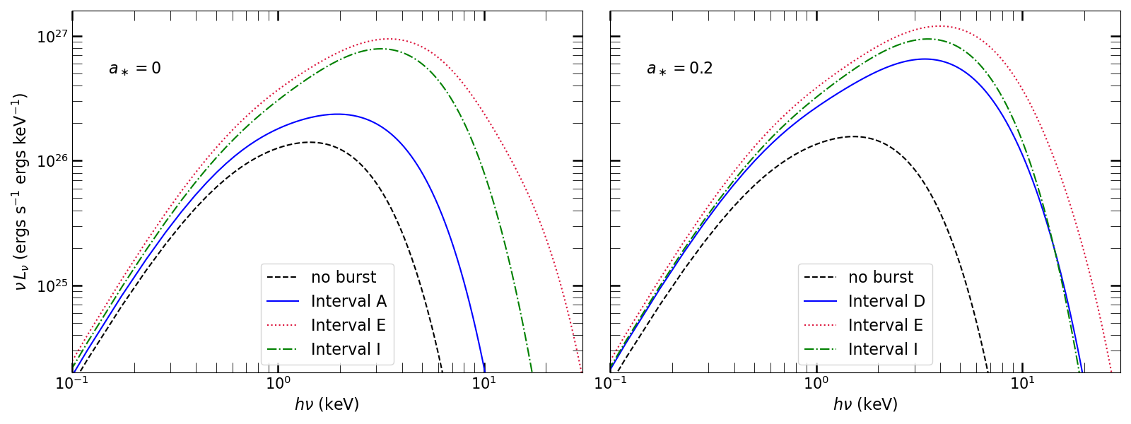
Figure 3: Left panel: Radially integrated disk spectra of the $a_{*}=0$ simulations. The spectra are integrated between the respective inner disk radius and 300 km (eq. 2). The time intervals and line styles are the same as in Fig. 2. Right panel: Same as the left panel, but for the $a_{*}=0.2$ simulations, and the spectra of time interval D instead of A being shown.

Fig. 3 shows integrated spectra (eq. 2) for time intervals A (blue solid line), E (red dotted line), and I (green dash-dotted line) for the $a_{*}=0$ burst simulation (left panel) and for time intervals D (blue solid line), E (red dotted line), and I (green dash-dotted line) for the $a_{*}=0.2$ burst simulation (right panel). Compared to the no-burst spectra of interval F (black solid lines), the disk spectra of both the $a_{*}=0$ and $a_{*}=0.2$ burst simulations are enhanced in magnitude and peak at higher energies. The enhanced magnitude and shift to higher energies is still present for the spectra of interval I due to the maintained high disk temperatures (Fig. 2). Furthermore, for a respective time interval, the $a_{*}=0.2$ spectrum has a greater amplitude than the $a_{*}=0$ spectrum due to the higher disk temperatures in the $a_{*}=0.2$ simulation.

2.2 Definition of $f_{a}$ and the mass accretion rate enhancement

To quantify the emission enhancement of the calculated spectra (eq. 2, Fig. 3), we utilize the normalization factor $f_{a}$. We calculate $f_{a}$ as the ratio between the maximum emission of the burst and the no-burst simulation,

$$f_{a}=\frac{\left(\nu L_{\nu}\right)_{\mathrm{max,\,b}}}{\left(\nu L_{\nu}\right)_{\mathrm{max,\,nb}}}.$$ (4)

The left panel of Fig. 4 shows the evolution of $f_{a}$ (eq. 4) for the $a_{*}=0$ (circle markers) and the $a_{*}=0.2$ (cross markers) burst simulation as a function of time. The marker size increases with time and the colors correspond to the time interval shadings in Fig. 1. The overplotted burst lightcurve (gray solid line, eq.1) shows that $f_{a}$ follows the burst evolution with some scatter for both spin configurations. For the $a_{*}=0$ simulation, $f_{a}$ is $\approx 1.7$ at interval A, reaches a maximum of $\approx 8.1$ at interval F, and is $\approx 5.6$ in interval I. In the $a_{*}=0.2$ burst simulation, $f_{a}\approx 4.2$ in time interval D, reaches a maximum of $\approx 7.7$ in interval E, and decreases to $\approx 6.1$ in interval I.

During the burst, the mass accretion rate also increases due to PR drag (Fragile et al., 2020; Speicher et al., 2023) We calculate the mass accretion rate enhancement $\dot{M}_{\mathrm{enh}}$ as the ratio of the time-averaged mass accretion rates between the burst and the no-burst simulations, measured at the respective $r_{\mathrm{isco}}$,

$$\dot{M}_{\mathrm{enh}}=\left.\frac{\left<\dot{M}_{\mathrm{b}}\right>}{\left<\dot{M}_{\mathrm{nb}}\right>}\right|_{r=r_{\mathrm{isco}}}.$$ (5)

The right panel of Fig. 4 shows the evolution of $\dot{M}_{\mathrm{enh}}$. The size and colors of the scatter points are the same as for the left panel. For the $a_{*}=0$ burst simulation, $\dot{M}_{\mathrm{enh}}$ is initially $\approx 1.6$ at interval A, reaches $\approx 9$ at the burst peak at interval E, and decreases to $\approx 1.6$ in the burst tail at interval I. In the $a_{*}=0.2$ burst simulation, the first considered time interval D has the highest $\dot{M}_{\mathrm{enh}}$ of $\approx 10.6$, decreasing slightly to $\approx 7.5$ at interval E and reaching $\approx 3.7$ in time interval I.

Figure 4: Left panel: The evolution of the normalization factor $f_{a}$, overplotted with the burst lightcurve (eq. 1, same as in Fig.1) for the $a_{*}=0$ (circle markers) and $a_{*}=0.2$ (cross markers) burst simulations. The size of the points in both panels increase with time. Their colors correspond to the shadings in Fig.1 for their respective time interval. With some scatter, $f_{a}$ follows the burst lightcurve for both simulations. Right panel: Same as the left panel, but showing the evolution of the mass accretion rate enhancement. Due to PR drag during the burst, $\dot{M}_{\mathrm{enh}}$ calculated at $r_{\mathrm{isco}}$ (eq. 5) increases in the $a_{*}=0$ burst simulation (circle markers) from $\approx 1.6$ to $\approx 9$ and decreases again to $\approx 1.6$. For the $a_{*}=0.2$ burst simulation (cross markers), $\dot{M}_{\mathrm{enh}}$ is $\approx 10.6$ in interval F, and decreases to $\approx 3.7$ in interval I.

3 Results

While the increase in the persistent emission captured by $f_{a}$ has been proposed to be connected to the $\dot{M}_{\mathrm{enh}}$ caused by PR drag, how well $f_{a}$ and $\dot{M}_{\mathrm{enh}}$ correlate remains unclear. In section 3.1, we examine the connection between $f_{a}$ and $\dot{M}_{\mathrm{enh}}$. Because $f_{a}$ has also been used to account for the soft excess, in Section 3.2 we investigate the contribution of the persistent emission to the soft excess.

3.1 Emission and mass accretion rate relationship

Figure 5: Left panel: Plot of $f_{a}$ versus $\dot{M}_{\mathrm{enh}}$ for the $a_{*}=0$ simulation. The colors are the same as in Fig. 1 and the marker sizes increase with time. $f_{a}$ and $\dot{M}_{\mathrm{enh}}$ are weakly linearly correlated, with a Pearson coefficient of $0.63$. Right panel: Same as the left panel, but for the $a_{*}=0.2$ simulation. Here, scatter affects the $f_{a}$ versus $\dot{M}_{\mathrm{enh}}$ relationship more significantly than for the $a_{*}=0$ simulation. The correlation between $\dot{M}_{\mathrm{enh}}$ and $f_{a}$ is only positive when restricting the time intervals E-I, with a correlation factor of $0.56$.

The relationship of $f_{a}$ versus $\dot{M}_{\mathrm{enh}}$ for the $a_{*}=0$ (left panel) and the $a_{*}=0.2$ (right panel) burst simulations can be seen in Fig. 5. For the $a_{*}=0$ simulation, a linear fit yields $\dot{M}_{\mathrm{enh}}=\left(0.9\pm 0.4\right)f_{a}+\left(-1.0\pm 2.4\right)$ and a Pearson correlation coefficient of $0.63$. Hence, $f_{a}$ and $\dot{M}_{\mathrm{enh}}$ are weakly related for the $a_{*}=0$ simulation.

Scatter affects the $f_{a}$ versus $\dot{M}_{\mathrm{enh}}$ relationship significantly more in the $a_{*}=0.2$ simulation (Fig. 5, right panel). Fitting a linear function yields $\dot{M}_{\mathrm{enh}}=\left(-0.6\pm 1.1\right)f_{a}+\left(11.1\pm 6.7\right)$ and a Pearson correlation coefficient of $-0.26$. The negative correlation is due to the large $\dot{M}_{\mathrm{enh}}$ despite a low $f_{a}$ in interval D. Ignoring this time interval and using only intervals E-I for fitting gives $\dot{M}_{\mathrm{enh}}=\left(2.0\pm 1.7\right)f_{a}+\left(-6.2\pm 11.4\right)$ and increases the Pearson correlation coefficient to $0.56$. For the $a_{*}=0$ burst simulation, restricting the fit to intervals E-I yields $\dot{M}_{\mathrm{enh}}=\left(1.6\pm 1.2\right)f_{a}+\left(-5.5\pm 7.7\right)$ and reduces the Pearson correlation coefficient slightly to $0.62$. Neglecting the burst rise, the slopes of the $f_{a}$ versus $\dot{M}_{\mathrm{enh}}$ relationships of the $a_{*}=0$ and $a_{*}=0.2$ simulations agree with each other within their uncertainties. However, the large uncertainties in slopes and the relatively low Pearson correlation coefficients ($\leq 0.63$) point towards a rather weak $f_{a}$ versus $\dot{M}_{\mathrm{enh}}$ relationship.

The weak $f_{a}$ versus $\dot{M}_{\mathrm{enh}}$ stems largely from the high temperatures in the burst tail, which decreases $f_{a}$ less than $\dot{M}_{\mathrm{enh}}$ (Fig. 4). In the $a_{*}=0$ simulation, $f_{a}$ increases from interval A to E by a factor of $4.02$ while $\dot{M}_{\mathrm{enh}}$ increases by a factor of $5.54$. However, as $\dot{M}_{\mathrm{enh}}$ decreases significantly again by a factor of $5.78$ between interval E and I, $f_{a}$ decreases only by a factor of $1.20$. Considering only intervals A-E of the $a_{*}=0$ simulation yields a correlation coefficient of $0.73$. Hence, $f_{a}$ and $\dot{M}_{\mathrm{enh}}$ are more correlated in the burst rise, and $f_{a}$ becomes more decoupled from the $\dot{M}_{\mathrm{enh}}$ evolution in the burst tail. Since $f_{a}$ follows the high disk temperatures in the burst tail rather than $\dot{M}_{\mathrm{enh}}$, $f_{a}$ correlates with temperature. Between $f_{a}$ and the disk temperature at $r_{in}$, we find a high Pearson correlation factor of $0.93$ for the $a_{*}=0$ simulation (based on intervals A-I) and $0.86$ for the $a_{*}=0.2$ simulation (based on intervals E-I). Because $f_{a}$ traces the disk temperature evolution, which especially in the burst tail does not represent $\dot{M}_{\mathrm{enh}}$, $f_{a}$ is not a reliable tracer of $\dot{M}_{\mathrm{enh}}$ in observations.

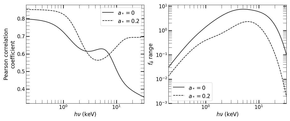
Figure 6: Left panel: Pearson correlation coefficient between $f_{\tilde{a}}$ (eq. 6) and $\dot{M}_{\mathrm{enh}}$ (eq. 5) as a function of energy. For both the $a_{*}=0$ (solid line) and $a_{*}=0.2$ (dashed line) simulations, $f_{\tilde{a}}$ correlates most strongly with $\dot{M}_{\mathrm{enh}}$ at energies below 1 keV. Right panel: The range of $f_{\tilde{a}}$ for the $a_{*}=0$ (solid line) and the $a_{*}=0.2$ (dashed line) simulations. With decreasing energy and beyond $\approx 10$ keV, $f_{\tilde{a}}$ varies less.

The weak $f_{a}$ versus $\dot{M}_{\mathrm{enh}}$ correlation changes with a different definition of the normalization factor (eq. 4). At energy $h\nu$, the redefined normalization factor called $f_{\tilde{a}}$ is the ratio between the emission at that energy of the burst simulation and the maximum emission of the no-burst simulation,

$$f_{\tilde{a}}(h\nu)=\frac{\left[\nu L_{\nu}(h\nu)\right]_{\mathrm{b}}}{\left[\nu L_{\nu}\right]_{\mathrm{max,\,nb}}}.$$ (6)

The left panel of Fig. 6 shows the Pearson correlation coefficients between $f_{\tilde{a}}$ and $\dot{M}_{\mathrm{enh}}$ at different energies. The correlation coefficient is based on time intervals A-I for the $a_{*}=0$ burst simulation (solid line). For the $a_{*}=0.2$ burst simulation (dashed line), only intervals E-I are used because the inclusion of interval D yielded significantly lower coefficients $\leq 0.36$. The correlation coefficients are highest at lower energies, reaching values up to $0.80$ for $a_{*}=0$ and $0.85$ for $a_{*}=0.2$. However, the range in $f_{\tilde{a}}$ decreases with decreasing energy for $h\nu\lesssim 10$ keV (Fig. 6, right panel). For example, at $0.51$ keV $f_{\tilde{a}}$ ranges between $0.58$ and $0.92$ for the $a_{*}=0$ simulation and between $0.71$ and $0.84$ for the $a_{*}=0.2$ simulation. The small range and values in $f_{\tilde{a}}$ at low energies differ from the $f_{a}$ inferred in observations (e.g., Worpel et al., 2015; Bult et al., 2022; Güver et al., 2022b), so the low energy $f_{\tilde{a}}$ are not a better representation of the observational $f_{a}$ compared to eq. 4. Hence, finding a high correlation between the low energy $f_{\tilde{a}}$ and $\dot{M}_{\mathrm{enh}}$ does not indicate that the observational $f_{a}$ factors would also have a high correlation as well. Obtaining these high coefficients in observational fits would require a redefinition of $f_{a}$. However, while $f_{\tilde{a}}$ correlates well with $\dot{M}_{\mathrm{enh}}$ at small energies, the small variation of $f_{\tilde{a}}$ at those energies might be challenging to measure in observations, especially if reflected and coronal emissions also extend to low energies (see section 4).

3.2 Impact of the spectral evolution on the soft excess

In addition to the emission enhancement, burst-induced disk heating shifts the calculated disk emission (Fig. 3) to higher energies. For the $a_{*}=0$ burst simulation, the spectral peak occurs at $\approx 0.5$ keV higher energy in time interval A than for the no-burst simulation spectrum. The spectral peak shift reaches $\approx 2.9$ keV in interval F (its maximum) and decreases to $\approx 1.7$ keV in interval I. The spectral peak is shifted similarly in the $a_{*}=0.2$ burst simulation. For time interval D, the spectral peak shift compared to its no-burst spectrum is $\approx 1.9$ keV, reaching its maximum of $\approx 2.5$ keV in interval E, and decreasing to $\approx 2.0$ keV in time interval I.

The shift of the disk emission to higher energies impacts its contribution to the soft excess, as shown in Fig. 7. Here, we define the soft excess as the disk emission surpassing the burst emission at energies $\lesssim 3$ keV. To calculate the burst emission, we assume it follows a blackbody with a blackbody temperature

$$T_{b}(t)=\left(\frac{L(t)}{4\pi\sigma_{b}R^{2}}\right)^{1/4}\left(1+z_{*}\right)^{-1},$$ (7)

where $\sigma_{b}$ is the Stefan–Boltzmann constant. The gravitational redshift $1+z_{*}$ is (Lewin et al., 1993),

$$1+z_{*}=\left(1-\frac{2GM}{Rc^{2}}\right)^{-1/2},$$ (8)

with $G$ being the gravitational constant. The burst spectrum is evaluated with the blackbody function,

$$B_{\nu}(T)=\frac{2h\nu^{3}}{c^{2}}\frac{1}{\exp\left[h\nu/kT_{b}\right]-1}.$$ (9)

Assuming the neutron star emits isotropically, the burst luminosity is $B_{\nu}$ multiplied by the redshifted neutron star surface area and $\pi$ (Rybicki & Lightman, 1986; Lewin et al., 1993):

$$L_{\nu,burst}=\left(\pi B_{\nu}(T)\right)\left[4\pi\left(1+z_{*}\right)^{2}R^{2}\right].$$ (10)

Note that these choices preserve the equality $4\pi\left(1+z_{*}\right)^{2}R^{2}\sigma_{b}T_{b}^{4}=4\pi\left(1+z_{*}\right)^{2}R^{2}\,\pi\int B_{\nu}\,d\nu$.

The top row of Fig. 7 shows the disk spectra for time interval E (red dotted lines, same as in Fig. 3) and the burst spectra (black solid lines) for the $a_{*}=0$ (left column) and $a_{*}=0.2$ (right column) simulations. Neither in time interval E nor during any other time interval does the disk emission surpass the burst emission at low energies, amounting to no contribution to a soft excess. Since we terminate the radial integration of the disk emission (eq. 2) at 300 km due to the outer simulation boundary, the shown spectra do not include the low-temperature emission of further out accretion disk regions. Including those would raise the emission at low energies and may generate a soft excess. However, the disk region beyond 300 km will not be significantly impacted by the burst radiation, so its luminosity will likely remain low and constant during the burst. Hence, even with an extension beyond 300 km, the disk emission is not expected to produce a strong soft excess.

The absence of a soft soft excess during the burst simulations is due to the evolution of the accretion disk spectra. The bottom row of Fig. 7 shows the no-burst disk spectra of interval F (red dashed lines) multiplied by the respective $f_{a}$ of time interval E. At energies $\lesssim 0.3$ keV, the scaled no-burst emission exceeds the burst emission (black solid lines) for both the $a_{*}=0$ (left panel) and $a_{*}=0.2$ (right panel) configurations, creating a soft excess. The spectral shape evolution to higher energies therefore reduces the accretion disk contribution to the soft excess.

To compare the soft excess from the disk emission to the soft excess due to reflection (Speicher et al., 2022), we calculate the percentage of soft excess below 3 keV as (Speicher et al., 2022)

$$\mathcal{S}=\frac{\int_{0.01\,\mathrm{keV}}^{3\,\mathrm{keV}}\left[F_{s}(E)-F_{bb}(E)\right]\,dE}{\int_{0.01\,\mathrm{keV}}^{3\,\mathrm{keV}}F_{s}(E)\,dE}\times 100,$$ (11)

with $F_{s}(E)$ being the disk emission and $F_{bb}(E)$ the burst emission as a function of energy $E$. The disk emission of the burst simulations (Fig. 7, top row) does not surpass the burst emission below 3 keV, yielding no positive $\mathcal{S}$ for any time intervals or spin configurations. For the scaled no-burst emission (Fig. 7, bottom row), we exclude instances where $F_{s}(E)-F_{bb}(E)<0$ when evaluating the integral in the numerator of eq. 11. Otherwise, $\mathcal{S}$ would also never be positive. Despite this modified calculation of $\mathcal{S}$, the percentage of soft excess is $\lesssim 0.2\%$ for all time intervals and spin configurations and thus negligible. Considering the strong soft excess due to reflection of up to $\approx 38\%$ found by Speicher et al. (2022), calculated using comparable simulation data (see also Fragile et al., 2020), these results imply that disk reprocessing is the main contributor to the soft excess.

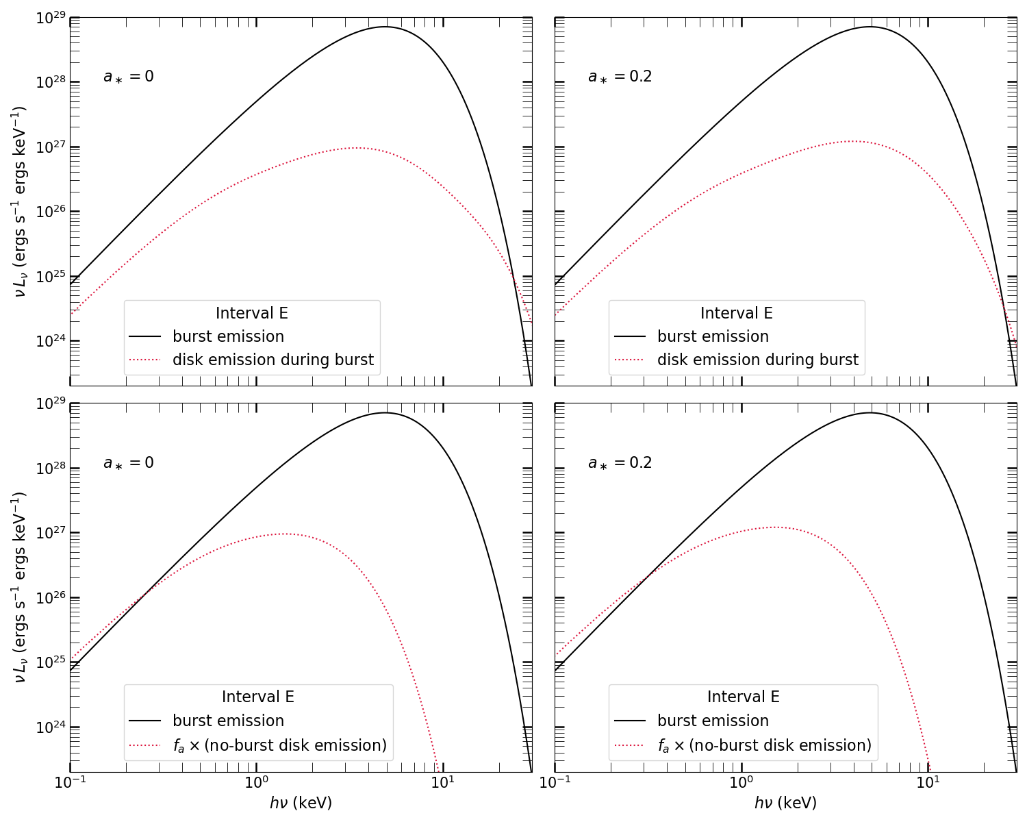
Figure 7: Top row: The disk spectra (red dotted lines, same as in Fig. 3) do not surpass the burst spectra (black solid lines) in time interval E for either the $a_{*}=0$ (left column) nor $a_{*}=0.2$ (right column) simulation, and thus do not contribute to a soft excess. Bottom row: Same as the top row, but instead of true disk spectra, no-burst spectra multiplied by $f_{a}$ are plotted. The scaled no-burst spectra exceed the burst spectra at low energies and generate an apparent soft excess. The disk spectra shifting to higher energies (top row) compared to them staying fixed in shape (bottom row) reduces their contribution to the soft excess.

4 Discussion

As varying the normalization of the accretion disk emission can improve the fit applied to burst observations, the $f_{a}$ factor has become a standard tool in the burst analysis repertoire. However, as shown in section 3, $f_{a}$ carries limited physical meaning. The normalization factor cannot accurately constrain $\dot{M}_{\mathrm{enh}}$ due to the relatively weak correlation of $f_{a}$ and $\dot{M}_{\mathrm{enh}}$. However, additional factors may further impact the correlation during real X-ray bursts, and are discussed in this section.

Burst properties will affect the $f_{a}$ versus $\dot{M}_{\mathrm{enh}}$ correlation. The burst photon energies impact the extent of disk heating and depend on the abundances in the atmosphere of the neutron star and its surface gravity (e.g., Suleimanov et al., 2011; Nättilä et al., 2015). Since disk heating affects $f_{a}$, its extent cannot only strengthen or weaken the $f_{a}$ vs $\dot{M}_{\mathrm{enh}}$ relationship, but also change its slope. Thus, neutron star systems can be expected to display a variety of $f_{a}$ vs $\dot{M}_{\mathrm{enh}}$ correlations, which will complicate constraining $\dot{M}_{\mathrm{enh}}$ using $f_{a}$.

In addition, the spectral evolution of the corona will impact $f_{a}$. In this paper, we focused on the spectral evolution of the accretion disk. However, the persistent emission also encompasses the emission of the corona, which radiates at high X-ray energies when not irradiated by an X-ray burst. During X-ray bursts, burst photons cool the corona (e.g., Fragile et al., 2018a; Speicher et al., 2020), leading to a drop in the observed hard X-ray emission (e.g., Maccarone & Coppi, 2003; Ji et al., 2014; Sánchez-Fernández et al., 2020). As the coronal emission at high X-ray energies decreases, the emission at low X-ray energies can increase depending on burst and coronal parameters (Speicher et al., 2020). An increase in soft coronal emission will increase $f_{a}$. While coronal cooling is accompanied by an increase in the mass accretion rate (Fragile et al., 2018a), the mass accretion rate evolution might be different in the corona compared to the accretion disk. Furthermore, the soft X-ray increase due to coronal cooling is not expected to trace the coronal accretion rate accurately because the emission increase depends on burst and coronal parameters. Hence, accounting for the coronal evolution during an X-ray burst will further cloud the $f_{a}$ versus $\dot{M}_{\mathrm{enh}}$ relationship further.

While the abovementioned factors complicate the $f_{a}$ versus $\dot{M}_{\mathrm{enh}}$ correlation, a different heating description could potentially strengthen it. The weak correlation largely stems from the high disk temperatures in the burst tail. Despite the receding burst luminosity in the tail, the burst radiation can still efficiently heat the disk. The high heating efficiency may be maintained by the evolving disk properties, such as a decreasing optical depth in the disk, which allows the burst radiation to heat deeper in the disk. Longer burst simulations are needed to fully decipher the disk evolution in the burst tail. In addition, accounting for magnetic fields in the disk structure could impact the thermodynamics of the disk (e.g., Sądowski, 2016) and this may avert the high disk temperatures maintained in the burst tail found here and therefore strengthen any $f_{a}$ versus $\dot{M}_{\mathrm{enh}}$ relationship. Numerical simulations of accretion disks impacted by X-ray bursts that follow the disk response through to the end of the burst are needed to better understand the thermal evolution of the disk.

5 Conclusions

X-ray spectral observations of Type I X-ray bursts are often fit with the persistent emission varying in magnitude, quantified with the normalization factor $f_{a}$ (e.g., Worpel et al., 2013, 2015; Bult et al., 2022). In addition, $f_{a}$ has been used to account for an often-observed soft excess (e.g., Keek et al., 2018; Güver et al., 2022a). The increase of $f_{a}$ is usually attributed to an increase in the mass accretion rate due to PR drag.

This paper examined the $f_{a}$ versus $\dot{M}_{\mathrm{enh}}$ relationship. With the simulation data of Speicher et al. (2023), we calculated the accretion disk emission during the burst evolution (section 2) and found that $f_{a}$ traces the disk temperature evolution but only shares a weak relationship with $\dot{M}_{\mathrm{enh}}$ (section 3.1), suggesting that $f_{a}$ cannot accurately capture $\dot{M}_{\mathrm{enh}}$ in observations (section 4).

Moreover, heating of the disk by the burst causes the disk emission to peak at increasingly higher energies, which reduces its contribution to the soft excess. The X-ray reflection spectra produced by the illuminated disk will therefore contribute more significantly to the soft excess than changes to the persistent emission (section 3.2). Therefore, X-ray reflection models appropriate for X-ray bursts (e.g., Ballantyne, 2004; García et al., 2022) should be used to account for any observed soft excesses found in the spectra of X-ray bursts.

To account for the spectral shape evolution, the disk emission could be fitted as a scaled multicolor blackbody with a varying temperature $T_{\mathrm{nb}}+\Delta T$, where $T_{\mathrm{nb}}$ is the temperature at $r_{in}$ with no burst (assuming the disk emission is fitted with the diskbb model by Makishima et al., 1986). Alternatively, a normalization factor focused solely on changes at low energy may give more insight into $\dot{M}_{\mathrm{enh}}$ (section 3.1). The current approach of scaling the persistent emission with $f_{a}$ will give an inaccurate picture of $\dot{M}_{\mathrm{enh}}$, as well as incorrectly classifying parts of the observed emission as originating from the accretion disk. In its current form, $f_{a}$ may provide some insight into the temperature of disk during an X-ray burst, although the complicated structural changes of the disk will limit its utility to accurately probe the details of the disk. Since the burst-disk interaction leads to a rich range of physical processes ongoing simultaneously (e.g., Ballantyne & Everett, 2005; Degenaar et al., 2018; Russell et al., 2024), spectral models motivated by the results of simulations such as these are likely the best strategy to infer the physical properties of the system.

References

- Abramowicz & Fragile (2013) Abramowicz, M. A., & Fragile, P. C. 2013, Living Reviews in Relativity, 16, 1, doi: 10.12942/lrr-2013-1
- Anninos et al. (2005) Anninos, P., Fragile, P. C., & Salmonson, J. D. 2005, ApJ, 635, 723, doi: 10.1086/497294
- Ballantyne (2004) Ballantyne, D. R. 2004, MNRAS, 351, 57, doi: 10.1111/j.1365-2966.2004.07767.x
- Ballantyne & Everett (2005) Ballantyne, D. R., & Everett, J. E. 2005, ApJ, 626, 364, doi: 10.1086/429860
- Ballantyne & Strohmayer (2004) Ballantyne, D. R., & Strohmayer, T. E. 2004, ApJ, 602, L105, doi: 10.1086/382703
- Barrière et al. (2015) Barrière, N. M., Krivonos, R., Tomsick, J. A., et al. 2015, ApJ, 799, 123, doi: 10.1088/0004-637X/799/2/123
- Bult et al. (2019) Bult, P., Jaisawal, G. K., Güver, T., et al. 2019, ApJ, 885, L1, doi: 10.3847/2041-8213/ab4ae1
- Bult et al. (2022) Bult, P., Mancuso, G. C., Strohmayer, T. E., et al. 2022, ApJ, 940, 81, doi: 10.3847/1538-4357/ac9b26
- Chen et al. (2022) Chen, Y.-P., Zhang, S., Ji, L., et al. 2022, ApJ, 936, 46, doi: 10.3847/1538-4357/ac87a0
- Degenaar et al. (2013) Degenaar, N., Miller, J. M., Wijnands, R., Altamirano, D., & Fabian, A. C. 2013, ApJ, 767, L37, doi: 10.1088/2041-8205/767/2/L37
- Degenaar et al. (2018) Degenaar, N., Ballantyne, D. R., Belloni, T., et al. 2018, Space Sci. Rev., 214, 15, doi: 10.1007/s11214-017-0448-3
- Done et al. (2012) Done, C., Davis, S. W., Jin, C., Blaes, O., & Ward, M. 2012, MNRAS, 420, 1848, doi: 10.1111/j.1365-2966.2011.19779.x
- Fragile et al. (2020) Fragile, P. C., Ballantyne, D. R., & Blankenship, A. 2020, Nature Astronomy, 4, 541, doi: 10.1038/s41550-019-0987-5
- Fragile et al. (2018a) Fragile, P. C., Ballantyne, D. R., Maccarone, T. J., & Witry, J. W. L. 2018a, ApJ, 867, L28, doi: 10.3847/2041-8213/aaeb99
- Fragile et al. (2018b) Fragile, P. C., Etheridge, S. M., Anninos, P., Mishra, B., & Kluźniak, W. 2018b, ApJ, 857, 1, doi: 10.3847/1538-4357/aab788
- Fragile et al. (2012) Fragile, P. C., Gillespie, A., Monahan, T., Rodriguez, M., & Anninos, P. 2012, ApJS, 201, 9, doi: 10.1088/0067-0049/201/2/9
- Fragile et al. (2014) Fragile, P. C., Olejar, A., & Anninos, P. 2014, ApJ, 796, 22, doi: 10.1088/0004-637X/796/1/22
- Galloway & Keek (2021) Galloway, D. K., & Keek, L. 2021, in Astrophysics and Space Science Library, Vol. 461, Timing Neutron Stars: Pulsations, Oscillations and Explosions, ed. T. M. Belloni, M. Méndez, & C. Zhang, 209–262, doi: 10.1007/978-3-662-62110-3_5
- Galloway et al. (2020) Galloway, D. K., in’t Zand, J., Chenevez, J., et al. 2020, ApJS, 249, 32, doi: 10.3847/1538-4365/ab9f2e
- García et al. (2022) García, J. A., Dauser, T., Ludlam, R., et al. 2022, ApJ, 926, 13, doi: 10.3847/1538-4357/ac3cb7
- Güver et al. (2022a) Güver, T., Bostancı, Z. F., Boztepe, T., et al. 2022a, ApJ, 935, 154, doi: 10.3847/1538-4357/ac8106
- Güver et al. (2022b) Güver, T., Boztepe, T., Ballantyne, D. R., et al. 2022b, MNRAS, 510, 1577, doi: 10.1093/mnras/stab3422
- Jaisawal et al. (2019) Jaisawal, G. K., Chenevez, J., Bult, P., et al. 2019, ApJ, 883, 61, doi: 10.3847/1538-4357/ab3a37
- Ji et al. (2014) Ji, L., Zhang, S., Chen, Y., et al. 2014, ApJ, 782, 40, doi: 10.1088/0004-637X/782/1/40
- Keek et al. (2017) Keek, L., Iwakiri, W., Serino, M., et al. 2017, ApJ, 836, 111, doi: 10.3847/1538-4357/836/1/111
- Keek et al. (2018) Keek, L., Arzoumanian, Z., Bult, P., et al. 2018, ApJ, 855, L4, doi: 10.3847/2041-8213/aab104
- Kubota et al. (2010) Kubota, A., Done, C., Davis, S. W., et al. 2010, ApJ, 714, 860, doi: 10.1088/0004-637X/714/1/860
- Kubota et al. (2005) Kubota, A., Ebisawa, K., Makishima, K., & Nakazawa, K. 2005, ApJ, 631, 1062, doi: 10.1086/432900
- Lewin et al. (1993) Lewin, W. H. G., van Paradijs, J., & Taam, R. E. 1993, Space Sci. Rev., 62, 223, doi: 10.1007/BF00196124
- Lu et al. (2024) Lu, Y., Li, Z., Yu, W., Pan, Y., & Falanga, M. 2024, ApJ, 969, 15, doi: 10.3847/1538-4357/ad4d86
- Maccarone & Coppi (2003) Maccarone, T. J., & Coppi, P. S. 2003, A&A, 399, 1151, doi: 10.1051/0004-6361:20021881
- Makishima et al. (1986) Makishima, K., Maejima, Y., Mitsuda, K., et al. 1986, ApJ, 308, 635, doi: 10.1086/164534
- Mitsuda et al. (1984) Mitsuda, K., Inoue, H., Koyama, K., et al. 1984, PASJ, 36, 741
- Nättilä et al. (2015) Nättilä, J., Suleimanov, V. F., Kajava, J. J. E., & Poutanen, J. 2015, A&A, 581, A83, doi: 10.1051/0004-6361/201526512
- Norris et al. (2005) Norris, J. P., Bonnell, J. T., Kazanas, D., et al. 2005, ApJ, 627, 324, doi: 10.1086/430294
- Peng et al. (2024) Peng, J. Q., Zhang, S., Chen, Y. P., et al. 2024, A&A, 685, A71, doi: 10.1051/0004-6361/202347534
- Robertson (1937) Robertson, H. P. 1937, MNRAS, 97, 423, doi: 10.1093/mnras/97.6.423
- Russell et al. (2024) Russell, T. D., Degenaar, N., van den Eijnden, J., et al. 2024, Nature, 627, 763, doi: 10.1038/s41586-024-07133-5
- Rybicki & Lightman (1986) Rybicki, G. B., & Lightman, A. P. 1986, Radiative Processes in Astrophysics
- Sánchez-Fernández et al. (2020) Sánchez-Fernández, C., Kajava, J. J. E., Poutanen, J., Kuulkers, E., & Suleimanov, V. F. 2020, A&A, 634, A58, doi: 10.1051/0004-6361/201936599
- Shakura & Sunyaev (1973) Shakura, N. I., & Sunyaev, R. A. 1973, A&A, 24, 337
- Sądowski (2016) Sądowski, A. 2016, MNRAS, 459, 4397, doi: 10.1093/mnras/stw913
- Speicher et al. (2022) Speicher, J., Ballantyne, D. R., & Fragile, P. C. 2022, MNRAS, 509, 1736, doi: 10.1093/mnras/stab3087
- Speicher et al. (2020) Speicher, J., Ballantyne, D. R., & Malzac, J. 2020, MNRAS, 499, 4479, doi: 10.1093/mnras/staa3137
- Speicher et al. (2023) Speicher, J., Fragile, P. C., & Ballantyne, D. R. 2023, MNRAS, 526, 1388, doi: 10.1093/mnras/stad2684
- Suleimanov et al. (2011) Suleimanov, V., Poutanen, J., & Werner, K. 2011, A&A, 527, A139, doi: 10.1051/0004-6361/201015845
- Suleimanov et al. (2012) —. 2012, A&A, 545, A120, doi: 10.1051/0004-6361/201219480
- Walker (1992) Walker, M. A. 1992, ApJ, 385, 642, doi: 10.1086/170969
- Walker & Meszaros (1989) Walker, M. A., & Meszaros, P. 1989, ApJ, 346, 844, doi: 10.1086/168065
- Worpel et al. (2013) Worpel, H., Galloway, D. K., & Price, D. J. 2013, ApJ, 772, 94, doi: 10.1088/0004-637X/772/2/94
- Worpel et al. (2015) —. 2015, ApJ, 801, 60, doi: 10.1088/0004-637X/801/1/60
- Yan et al. (2024) Yan, Z., Zhang, G., Chen, Y.-P., et al. 2024, MNRAS, 529, 1585, doi: 10.1093/mnras/stae283
- Yu et al. (2024) Yu, W., Li, Z., Lu, Y., et al. 2024, A&A, 683, A93, doi: 10.1051/0004-6361/202348195
- Zdziarski et al. (2022) Zdziarski, A. A., You, B., & Szanecki, M. 2022, ApJ, 939, L2, doi: 10.3847/2041-8213/ac9474
- Zhao et al. (2022) Zhao, G., Li, Z., Pan, Y., et al. 2022, A&A, 660, A31, doi: 10.1051/0004-6361/202142801