OTFS-MDMA: An Elastic Multi-Domain Resource Utilization Mechanism for High Mobility Scenarios

Abstract

By harnessing the delay-Doppler (DD) resource domain, orthogonal time-frequency space (OTFS) substantially improves the communication performance under high-mobility scenarios by maintaining quasi-time-invariant channel characteristics. However, conventional multiple access (MA) techniques fail to efficiently support OTFS in the face of diverse communication requirements. Recently, multi-dimensional MA (MDMA) has emerged as a flexible channel access technique by elastically exploiting multi-domain resources for tailored service provision. Therefore, we conceive an elastic multi-domain resource utilization mechanism for a novel multi-user OTFS-MDMA system by leveraging user-specific channel characteristics across the DD, power, and spatial resource domains. Specifically, we divide all DD resource bins into separate subregions called DD resource slots (RSs), each of which supports a fraction of users, thus reducing the multi-user interference. Then, the most suitable MA, including orthogonal, non-orthogonal, or spatial division MA (OMA/ NOMA/ SDMA), will be selected with each RS based on the interference levels in the power and spatial domains, thus enhancing the spectrum efficiency. Then, we jointly optimize the user assignment, access scheme selection, and power allocation in all DD RSs to maximize the weighted sum-rate subject to their minimum rate and various practical constraints. Since this results in a non-convex problem, we develop a dynamic programming and monotonic optimization (DPMO) method to find the globally optimal solution in the special case of disregarding rate constraints. Subsequently, we apply a low-complexity algorithm to find sub-optimal solutions in general cases.

I Introduction

Next-generation cellular systems are expected to provide reliable communications for a massive number of users [1, 2, 3]. This is particularly challenging for the dynamic channels encountered in high-mobility scenarios of aircraft-to-ground communications, industrial automation, intelligent transportation, etc. Conventional multi-carrier modulation techniques, such as orthogonal frequency division multiplexing (OFDM), suffer from performance degradation in high-mobility scenarios due to the doubly selective channels with substantial delay-Doppler spreads [4]. On the other hand, conventional multiple access (MA) schemes such as frequency division, time division, spatial division, or non-orthogonal MA (FDMA, TDMA, SDMA, NOMA) have inherent limitations in terms of accommodating numerous users with high spectrum efficiency, which lacks flexibility in terms of supporting diverse users due to the rigid utilization of a single resource domain. This motivates us to investigate novel elastic multi-dimensional modulation and access mechanisms to fulfill diverse user demands in mobile communications.

Orthogonal time-frequency space (OTFS) modulation has demonstrated superior performance compared to traditional multi-carrier modulation methods in high-mobility scenarios [5, 6, 7, 8, 9]. This is because OTFS maps the data symbols to the two-dimensional delay-Doppler (DD) resource domain, and each path of a doubly-selective channel with specific delay and Doppler spreads can be represented by a specific quasi-time-invariant channel tap on the DD plane. Consequently, the received OTFS signals can be viewed as a two-dimensional convolution between the information symbols and the effective DD domain channel. This scheme harnesses both the frequency- and time-diversity of doubly-selective channels, enabling reliable communication [10]. Moreover, despite the complexity challenges associated with OTFS [11], its time-invariant channel characteristics in the DD domain facilitate stable resource allocation in mobility scenarios, making it more promising than OFDM facing time-varying channels, particularly in multi-user cases. This advantage arises because adapting resource allocation for time-varying channels increases both design complexity and control overhead for exchanging updated allocation schemes between transceivers. References [12, 13] demonstrate that as the degrees of freedom in the optimization variables increase, the performance gap between OTFS and OFDM becomes more pronounced.

Due to its promising potential, OTFS modulation has garnered significant attention recently from both industry and academia. Specifically, a simple matrix representation of the input-output relationship of OTFS modulation using practical pulse-shaping waveforms was developed in [14]. The resultant relationship exhibits a sparse structure, which facilitates the implementation of sophisticated detection algorithms having low computational complexity. Then, a simplified linear minimum mean square error receiver was introduced in [15], which utilizes the sparse nature of the channel and the quasi-band structure of the matrices in the demodulation process to reduce the decoding complexity. The authors of [16] introduced an iterative interference canceller and detector that employs message passing for joint inter-Doppler and inter-carrier interference cancellation as well as symbol detection. Then, this detector was extended in [17] by using unitary approximate techniques and exploiting the structured nature of the channel matrix. Furthermore, the channel sparsity was exploited to devise a Bayesian learning framework for estimating DD domain channels for single-input single-output (SISO) [18] and multiple-input multiple-output (MIMO) [19] systems.

As expected, there is already literature investigating OTFS systems relying on various MA technologies. Specifically, for single-antenna OTFS systems [20, 21, 22, 23, 24, 25], the classical orthogonal MA (OMA) methods were investigated in [20, 21], where users are assigned distinct delay, Doppler, or frequency resource bins to reduce co-channel interference. Besides, [20] found that interleaved DD domain OMA offers better spectral efficiency than interleaved time-frequency (TF) domain OMA. Then, power-domain NOMA was investigated in [22, 23] to enable non-orthogonal spectrum sharing between high-mobility and low-mobility users. The sophisticated equalization and message-passing algorithms were utilized in [22] and [23], respectively, to achieve efficient OTFS signal reception. In [24], a sparse code MA (SCMA) scheme was conceived for the uplink of coordinated multi-point vehicular networks, where the performance was improved by leveraging additional diversity from both the Doppler and spatial domains. Next, a tandem spreading MA (TSMA) arrangement was introduced in [25] for a large-scale network, where segment coding and tandem spreading methods were deployed to improve both connectivity and reliability by sacrificing the data rate. Later, for multi-antenna OTFS systems [26, 27], path division MA (PDMA) was proposed in [26] for both uplink and downlink by allocating angle-domain resources for multiple users to avoid co-channel interference. As a further advance, a deep learning-based predictive precoder design was proposed in [27] to enable ultra-reliable low-latency communications.

Topics	Paper	OTFS	MA Scheme	BS Antenna	Characteristics
OTFS-MA	[20, 21]	$\checkmark$	OMA	Single	$\bullet$ Single-domain resource allocatioin $\bullet$ Fixed MA scheme
	[22, 23]	$\checkmark$	power-domain NOMA	Single
	[24]	$\checkmark$	SCMA	Single
	[25]	$\checkmark$	TSMA	Single
	[26]	$\checkmark$	PDMA	Multiple
	[27]	$\checkmark$	SDMA	Multiple
MDMA	[28, 29]	$\texttimes$	OMA, power/spatial-domain NOMA	Multiple	$\bullet$ Adaptive MA for stationary channels
	[30]	$\texttimes$	OMA, power/spatial/hybrid-domain NOMA	Multiple
OTFS- MDMA	Our	$\checkmark$	OMA/NOMA/SDMA	Multiple	$\bullet$ Elastic multi-domain resource allocation $\bullet$ Adaptive MA for mobility channels

TABLE I: Recent advances in OTFS and MDMA systems

Nonetheless, the aforementioned studies exclusively concentrate on a single-domain or fixed access scheme, thereby exhibiting inherent limitations in terms of enhancing spectral efficiency. As a remedy, the multi-dimensional MA (MDMA) method may be regarded as a promising MA technique[3]. Explicitly, MDMA is a hybrid multiple-access technology capable of flexibly apportioning interference levels across various radio resource domains by beneficially integrating different types of MA methods (orthogonal or non-orthogonal). Thus flexible channel access is capable of increasing the number of users while supporting diverse high quality-of-services (QoSs). Specifically, the authors of [28],[29] explored how the non-orthogonality introduced by NOMA and SDMA affects the resource utilization costs in various radio resource domains. They dynamically switched between OMA, power-domain NOMA, and spatial-domain NOMA to maximize the cost-aware system throughput. Then, these solutions were extended in [30], where a hybrid spatial- and power-domain NOMA was proposed to glean additional resource diversity for performance enhancement. They carefully considered the user-specific resource availability and the resource exploitation capability to strike a balance between the resource utilization cost and the performance gain. However, these studies only address MDMA designs for stationary wireless channels. Hence, their solutions suffer from significant performance degradation in high-mobility scenarios of future cellular systems.

Against the above backdrop, also summarized in Table I, we highlight our main contributions as follows:

• We develop an elastic multi-domain resource utilization mechanism for multi-user OTFS-MDMA systems, which leverages the time-invariant user-specific channel characteristics across the DD, power, and spatial domains to facilitate flexible channel access and resource allocation, thereby enabling efficient varied service provisions.

• We conceive a novel DD domain division and user accommodation scheme, where the DD resource bins are partitioned into separate subregions called resource slots (RSs), and each RS is associated with a specific group of users based on their channel characteristics, thus reducing multi-user interference. This is termed as DD domain user accommodation. Then, the most suitable MA techniques, including OMA/NOMA/SDMA, are applied for each RS based on their interference levels in the power and spatial domains, thus increasing the spectrum efficiency.

• We jointly optimize the user accommodation, access scheme selection, and power allocation for maximizing the weighted sum-rate of all users subject to individual minimum rate constraints and various practical constraints. Since the problem formulated belongs to the mixed integer nonlinear programming (MINLP) family, we develop an optimal algorithm based on dynamic programming and monotonic optimization (DPMO) for the problem in the special case of disregarding individual rate constraints. Subsequently, we propose a low-complexity successive convex approximation-based simulated annealing (SCA-SA) algorithm to obtain a sub-optimal solution to the original problem in general cases.

• Simulation results show that the proposed sub-optimal algorithm approaches the performance of the optimal algorithms, and significantly outperforms other baselines.

Organizations: Sections II and III introduce the OTFS-MDMA system model and problem formulation, respectively. Section IV develops the optimal solution for the relaxed problem and Section V develops the sub-optimal algorithm for the original problem. Finally, Section VI provides simulation results and Section VII concludes the paper.

Notations: The scalar, vector, and matrix using lowercase, bold lowercase, and bold uppercase letters are represented by $x$, $\mathbf{x}$, and $\mathbf{X}$, respectively. The transpose, conjugate transpose, diagonalization, Kronecker product, vectorization, inverse vectorization, and Dirac delta function are denoted by $(\cdot)^{T}$, $(\cdot)^{H}$, ${\rm diag}(\cdot)$, $\otimes$, ${\rm vec}(\cdot)$, ${\rm vec}^{-1}(\cdot)$, and $\delta(\cdot)$, respectively. Moreover, we let ${{\bf{F}}_{X}}=\left\{{\frac{1}{{\sqrt{X}}}{e^{j2\pi\frac{{kl}}{X}}}}\right\}_{k,l=0}^{X-1}$ be the $X$-point DFT matrices. Finally, $\left|{\cal R}\right|$ denotes the number of elements in set $\cal R$ and ${\bf 1}_{R}$ represents a size $R$ vector with all elements as 1.

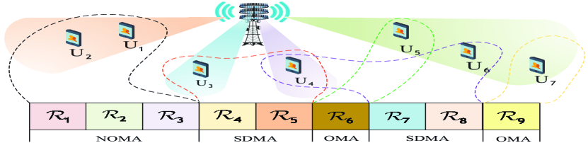
(a) DD domain user accommodation with MDMA

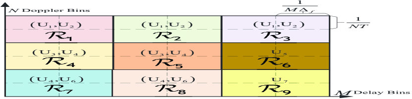
(b) DD domain division with $R=9$ resource slot (RS), each of which includes ${\left|{{{{\cal R}}_{r}}}\right|}=\delta_{M}\delta_{N}=4$ resource bins

Figure 1: Illustration of user accommodation in the DD domain in a multi-user MISO OTFS-MDMA system.

II System Model

As shown in Fig. 1, we consider a multi-user multiple-input single-output (MISO) OTFS-MDMA system, where a BS equipped with $D$ antennas broadcasts individual OTFS modulated signals to $Q$ single-antenna users, denoted by ${\rm U}_{1},\cdots,{\rm U}_{Q}$. We assume all channels are time-invariant in the DD domain during each transmission frame and the channel knowledge is perfectly known at the BS for the system design. Then, by exploiting different degrees of orthogonality and interference of channels across the DD, power, and spatial domains, we develop the OTFS-MDMA scheme. Specifically, all DD resource bins are divided into multiple non-overlapping subregions called resource slots (RSs). Taking into account the individual channel characteristics of each user in the multi-dimensional resource domains, we assign specific groups of users to distinct RSs, which is called DD domain user accommodation. Then, we apply MDMA to these RSs to achieve information transmission for these users. This involves choosing the most suitable MA schemes from different resource domains, including NOMA and SDMA/OMA, tailored to each RS for enhancing spectral efficiency. Intuitively, the NOMA scheme is preferred by users equipped with powerful hardware for self-interference cancellation (SIC) and whose channels are highly correlated in the spatial domain, where the co-channel interference remains significant despite its mitigation by beamforming. On the other hand, users having limited computational capabilities and orthogonal channels may opt for SDMA/OMA to achieve improved capacity at low complexity and interference.

II-A DD Domain User Accommodation

In the DD domain, $MN$ data symbols are embedded in the two-dimensional $M\times N$ DD resource bins, where $M$ and $N$ denote the number of delay bins (or subcarriers) and the number of Doppler bins (or time intervals), respectively. The subcarrier bandwidth and symbol duration are denoted by $\Delta_{f}$ and $T=1/\Delta_{f}$, respectively. Let the $b$-th resource bin represent the resource bin associated with the $(k+1)$-th Doppler bin (i.e., $\frac{k}{NT}$) and the $(l+1)$-th delay bin (i.e., $\frac{l}{M\Delta_{f}}$), where ${b}=kM+l+1$ for $0\leq k\leq N-1$ and $0\leq\l\leq M-1$. As illustrated in Fig. 1 (b), we assume that $M\times N$ DD resource bins are equally partitioned into $R$ RSs for simplicity, i.e., ${\cal R}_{1},{\cal R}_{2},\cdots,{\cal R}_{R}$, and each RS is characterized by lengths of $\delta_{M}$ and $\delta_{N}$. We assume that ${M}/{{{\delta_{M}}}}$ are ${N}/{{{\delta_{N}}}}$ are integers, and we know that $R=\frac{{MN}}{{{\delta_{M}}{\delta_{N}}}}$, ${\left|{{{{\cal R}}_{r}}}\right|}=\delta_{M}\delta_{N}$, $\sum\nolimits_{r=1}^{R}{\left|{{{{\cal R}}_{r}}}\right|}=MN$, and $\bigcup\nolimits_{r=1}^{R}{{{\cal R}_{r}}}=\left\{{1,\cdots,b,\cdots,MN}\right\}$.

Next, a subset of users is accommodated in RS ${\cal R}_{r}$, where the choice of using NOMA or SDMA/OMA is based on the channel orthogonality among these users across the DD, power, and spatial domains. Since increasing the number of users in the same RS increases both the interference and also the decoding complexity and delay in the NOMA scheme, we assume that each RS ${\cal R}_{r}$ only accommodates two users for NOMA [31, 32], but the maximum of $Q$ users for SDMA. Here, OMA can be regarded as a special case of SDMA if there is only a single user in an RS.

Then, let $a_{rqi}^{\rm N}$ and $a^{\rm S}_{r}$ denote binary variables involving user accommodation decisions and MA scheme selections, i.e., $a_{rqi}^{\rm N}=1$ means that users ${\rm U}_{q}$ and ${\rm U}_{i}$ are accommodated in ${\cal R}_{r}$ using NOMA, otherwise $a_{rqi}^{\rm N}=0$. Besides, $a_{r}^{\rm S}=1$ means that users are accommodated in ${\cal R}_{r}$ using SDMA/OMA, otherwise $a_{r}^{\rm S}=0$. Then, let the data symbol of user ${\rm U}_{q}$ transmitted in the $b$-th resource bin be $x_{qb}$. Thus, the $b$-th DD domain data symbol in RS ${{\cal R}_{r}}$ transmitted through the $d$-th antenna before multiplexing with the aid of the transmit precoding matrix is

$$x_{{\rm{DD}}}^{d}\left[b\right]=\left\{{\begin{array}[]{*{20}{l}}{\sqrt{{p_{qb}}}w_{qb}^{d}{x_{qb}}+\sqrt{{p_{ib}}}w_{ib}^{d}{x_{ib}},\;{\rm{if}}\;a_{rqi}^{\rm{N}}=1},\\ {\sum\nolimits_{q=1}^{Q}{\sqrt{{p_{qb}}}w_{qb}^{d}{x_{qb}}},\;{\rm{if}}\;a_{r}^{\rm{S}}=1{\rm{}},}\end{array}}\right.$$ (3)

for $b\in{\cal R}_{r}$ and $\forall r$, where $w_{qb}^{d}$ is the $d$-th element of the transmit beamforming vector ${\bf w}_{qb}\in{\mathbb{C}}^{D\times 1}$ with normalized power for the information transmission of ${\rm U}_{q}$ at the $b$-th DD resource bin. Besides, $p_{qb}$ is the corresponding transmission power.

II-B OTFS Transmit Signal Model

In this part, we introduce the OTFS downlink transmission signal model. By rewriting $x_{{\rm{DD}}}^{d}\left[b\right]$ $(1\leq b\leq MN)$ into the vectorial form, i.e., ${{\bf{x}}^{d}_{\rm{DD}}}\in{\mathbb{C}}^{MN\times 1}$ and denoting the transmit precoding matrix by ${\bf P}_{\rm tx}\in{{\mathbb{C}}^{MN\times MN}}$, we have the following symbol matrix, i.e.,

$${{\bf{\tilde{X}}}_{{\rm{DD}}}^{d}}={\rm{ve}}{{\rm{c}}^{-1}}\left({{\bf P}_{\rm tx}{{\bf{x}}^{d}_{\rm{DD}}}}\right)\in{{\mathbb{C}}^{N\times M}}.$$ (4)

By applying the inverse symplectic finite Fourier transform (SFFT), these data symbols in the TF domain transmitted through the $d$-th antenna can be represented by

$${S}^{d}_{\rm{TF}}\left[{n,m}\right]=\frac{1}{\sqrt{MN}}\sum\limits_{k=0}^{N-1}{\sum\limits_{l=0}^{M-1}{{{\tilde{x}}^{d}_{\rm{DD}}}\left[{k,l}\right]{e^{{\rm{j}}2\pi\left({\frac{{kn}}{N}-\frac{{ml}}{M}}\right)}}}},$$ (5)

where ${{\tilde{x}}^{d}_{\rm{DD}}}\left[{k,l}\right]$ is the $(k,l)$-th element of ${{\bf{\tilde{X}}}_{{\rm{DD}}}^{d}}$. Then, by applying the Heisenberg transform to the transmit waveform $G_{\rm tx}(t)$, the TF domain signals ${S}^{d}_{\rm{TF}}\left[{n,m}\right]$ can be transformed into a continuous waveform in the time domain, yielding:

$$s^{d}\left(t\right)$$

$$= \sum\limits_{n=0}^{N-1}{\sum\limits_{m=0}^{M-1}{S^{d}_{\rm{TF}}\left[{n,m}\right]}}{G_{\rm tx}}\left(t-nT\right){e^{j2\pi m{\Delta_{f}}\left({t-nT}\right)}}.$$ (6)

II-C Channel Model

Let $h_{q}^{d}\left(\tau,\nu\right)$ denote the channel response between the $d$-th antenna at the BS and user ${\rm U}_{q}$ in the DD domain. This channel response comprises $L_{q}$ propagation paths, each with distinct delay $\tau_{q,\ell}$, Doppler shift $\upsilon_{q,\ell}$, and angle of departure $\theta_{q,\ell}$, formulated as

$${h_{q}^{d}}\left({\tau,\upsilon}\right)$$

$$= \sum\nolimits_{\ell=1}^{{L_{q}}}{\frac{h_{q,\ell}}{\sqrt{L_{q}}}{{e^{-j\pi\sin{\theta_{q,\ell}}\left({d-1}\right)}}}\delta\left({\tau-{\tau_{q,\ell}}}\right)}\delta\left({\upsilon-{\upsilon_{q,\ell}}}\right),$$ (7)

where $h_{q,\ell}$ is the complex channel response of the $\ell$-th propagation path arriving from the BS to user ${\rm U}_{q}$. Furthermore, ${\tau_{q,\ell}}$ and ${\upsilon_{q,\ell}}$ can be represented by ${\tau_{q,\ell}}=\frac{{{l_{q,\ell}}}}{{M{\Delta_{f}}}}$ and ${\upsilon_{q,\ell}}=\frac{{{k_{q,\ell}}+{{\tilde{k}}_{q,\ell}}}}{{NT}}$, respectively, where ${l_{q,\ell}}$ and ${k_{q,\ell}}$ are integers representing the indices of ${\tau_{q,\ell}}$ and ${\upsilon_{q,\ell}}$, respectively. The real parameter $-0.5\leq{\tilde{k}_{q,\ell}}\leq 0.5$ denotes the fraction of Doppler phase shift from the nearest integer ${k_{q,\ell}}$. Here, the fractional delay can be ignored due to the high-resolution sampling time $\frac{1}{M\Delta_{f}}$ [17].

II-D OTFS Receive Signal Model

From (7), the signal received in the time domain at user $q$ upon transmitting $\left\{s^{d}\left(t\right),1\leq d\leq D\right\}$ through $D$ antennas is formulated as:

$$y_{q}\left(t\right)$$

$$= \int{\!\int{\sum\limits_{d=1}^{D}{h_{q}^{d}\left({\tau,\upsilon}\right){s^{d}}\left({t\!-\!\tau}\right){e^{j2\pi\upsilon\left({t-\tau}\right)}}}}}{{\rm{d}}_{\tau}}{{\rm{d}}_{\upsilon}}+u_{q}\left(t\right),$$ (8)

where $u_{q}\left(t\right)$ is the complex additive white Gaussian noise.

Upon denoting the receive waveform by ${G_{\rm rx}}\left({t}\right)$, the signal received at user ${\rm U}_{q}$ in the TF domain becomes:

$${Y_{\rm TF}^{q}}\left[{n,m}\right]=\int{{y_{q}}}\left(t\right){G_{\rm rx}}\left({t-nT}\right){e^{j2\pi m{\Delta_{f}}\left({t-nT}\right)}}{{\rm{d}}_{t}}.$$ (9)

Next, we assume that ${G}_{\rm tx}(t)$ and ${G}_{\rm rx}(t)$ satisfy the bi-orthogonal property, which can eliminate cross-symbol interference during symbol reception. This assumption provides an upper bound on the performance of OTFS with other waveforms, such as rectangular waveforms [6, 16]. By applying the SFFT to ${Y_{\rm TF}^{q}}\left[{n,m}\right]$, the channel’s input-output relationship in the DD domain is expressed as:

$$y_{{\rm{DD}}}^{q}\left[{k,l}\right]= \frac{1}{{\sqrt{MN}}}\sum\nolimits_{n=0}^{N-1}{\sum\nolimits_{m=0}^{M-1}{Y_{{\rm{TF}}}^{q}\left[{n,m}\right]{e^{-{\rm{j}}2\pi\left({\frac{{nk}}{N}-\frac{{ml}}{M}}\right)}}}}$$

$$= \frac{1}{{MN}}\sum\nolimits_{n=0}^{N-1}{\sum\nolimits_{m=0}^{M-1}{\left({\sum\nolimits_{d=1}^{D}{\tilde{x}_{{\rm{DD}}}^{d}\left[{n,m}\right]}}\right.}}$$

$$\times\left.{\tilde{h}_{q}^{d}\left[{{{\left({k-n}\right)}_{N}},{{\left({l-m}\right)}_{M}}}\right]}\right)+{u_{q}}\left[{k,l}\right],$$ (10)

where ${u_{q}}\left[{k,l}\right[$ is the noise term and $\tilde{h}_{q}^{d}\left({k,l}\right)$ is given by

$$\tilde{h}_{q}^{d}\left({k,l}\right)=\sum\limits_{\ell=1}^{{L_{q}}}{h_{q,\ell}^{d}{e^{-j2\pi{\nu_{q,\ell}}{\tau_{q,\ell}}}}\phi\left({k-{k_{q,\ell}},l-{l_{q,\ell}}}\right)},$$ (11)

with $h_{q,\ell}^{d}={h_{q,\ell}}{e^{-j\pi\sin{\theta_{q,\ell}}\left({d-1}\right)}}$ and $\phi\left({k-{k_{q,\ell}},l-{l_{q,\ell}}}\right)=\sum\nolimits_{n^{\prime}=0}^{N-1}{\sum\nolimits_{m^{\prime}=0}^{M-1}{{e^{-{\rm{j}}2\pi\left({n^{\prime}\frac{{k-{k_{q,\ell}}-{{\tilde{k}}_{q,\ell}}}}{N}-m^{\prime}\frac{{l-{l_{q,\ell}}}}{M}}\right)}}}}$. Following a similar approximation of [16], $y_{{\rm{DD}}}^{q}\left[{k,l}\right]$ is rewritten by

$$y_{{\rm{DD}}}^{q}\left[{k,l}\right]\!\approx \!\sum\limits_{d=1}^{D}{\sum\limits_{\ell=1}^{{L_{q}}}{\sum\limits_{i=-{N_{q,\ell}}}^{{N_{q,\ell}}}{\left({\tilde{x}_{{\rm{DD}}}^{d}\left[{{{\left({k\!-\!{k_{q,\ell}}\!+\!i}\right)}_{N}},{{\left({l\!-\!{l_{q,\ell}}}\right)}_{M}}}\right]}\right.}}}$$

$$\times\left.{\bar{h}_{q,\ell,i}^{d}{e^{-j2\pi{\nu_{q,\ell}}{\tau_{q,\ell}}}}}\right)+{u_{q}}\left[{k,l}\right],$$ (12)

where $\bar{h}_{q,\ell,i}^{d}=h_{q,\ell}^{d}\left({\frac{{{e^{-{\rm{j}}2\pi\left({-i-{\tilde{k}_{q,\ell}}}\right)}}-1}}{{N{e^{-{\rm{j}}\frac{{2\pi}}{N}\left({-i-{\tilde{k}_{q,\ell}}}\right)}}-N}}}\right)$. Here, $N_{q,\ell}\ll N$ is a small number, considering the significant values of $\phi\left({k-{k_{q,\ell}},l-{l_{q,\ell}}}\right)$ around the peak at $k-k_{q,\ell}$.

Then, upon denoting the vectorial versions of $y_{{\rm{DD}}}^{q}\left[{k,l}\right]$ and $\tilde{x}_{{\rm{DD}}}^{q}\left[{k,l}\right]$ by ${{\bf{y}}^{q}_{\rm DD}}\in{\mathbb{C}}^{MN\times 1}$ and ${{\bf{\tilde{x}}}^{q}_{\rm DD}}\in{\mathbb{C}}^{MN\times 1}$, we rewrite (12) into the following matrix form [17]

$${{\bf{y}}^{q}_{\rm DD}}=\sum\nolimits_{d=1}^{D}{{\bf{H}}_{q}^{d}}{\bf{\tilde{x}}}^{d}_{{{\rm{DD}}}}+{{\bf{u}}^{q}_{\rm DD}},$$ (13)

where ${{\bf{u}}^{q}_{\rm DD}}\in{\mathbb{C}}^{MN\times 1}$ is the vectorial version of ${u_{q}}\left[{k,l}\right]$, and ${{\bf{H}}_{q}^{d}}\in{\mathbb{C}}^{MN\times MN}$ is given by

$${\bf{H}}_{q}^{d} =\sum\nolimits_{\ell=1}^{{L_{q}}}{\sum\nolimits_{i=-{N_{q,\ell}}}^{{N_{q,\ell}}}{\left({\bar{h}_{q,\ell,i}^{d}{e^{-j2\pi\frac{{\left({{k_{q,\ell}}+{{\tilde{k}}_{q,\ell}}}\right){l_{q,\ell}}}}{{MN}}}}}\right.}}$$

$$\qquad\times\left.{{{\bf{I}}_{N}}\left({-{{\left[{i-{k_{q,\ell}}}\right]}_{N}}}\right)\otimes{{\bf{I}}_{M}}\left({{l_{q,\ell}}}\right)}\right).$$ (14)

Here, ${{\bf{I}}_{N}}\left({-{{\left[{i-{k}}\right]}_{N}}}\right)$ is the matrix obtained upon circularly shifting the rows of the $N\times N$ identity matrix by $-[i-k]_{N}$, and ${{\bf{I}}_{M}}\left({{l_{q,\ell}}}\right)\in{\mathbb{C}}^{M\times M}$ is defined similarly. For the special case of no fractional Doppler phase shift, we have

$${\bf{H}}_{q}^{d}=\sum\nolimits_{\ell=1}^{{L_{q}}}{h_{q,\ell}^{d}{e^{-j2\pi\frac{{{{k_{q,\ell}}}{l_{q,\ell}}}}{{MN}}}}}{{\bf{I}}_{N}}\left({{k_{q,\ell}}}\right)\otimes{{\bf{I}}_{M}}\left({{l_{q,\ell}}}\right).$$ (15)

Note that regardless of whether there are fractional Doppler phase shifts, ${\bf H}_{q}^{d}$ is a block circulant matrix [17], which can be formulated by ${\bf H}_{q}^{d}={\rm{circ}}\left[{{{\bf{G}}_{q,0}^{d}},{{\bf{G}}_{q,1}^{d}},\cdots{{\bf{G}}_{q,N-1}^{d}}}\right]\in{\mathbb{C}}^{NM\times NM}$, i.e.,

$${\bf{H}}_{q}^{d}=\left[{\begin{array}[]{*{20}{c}}{{\bf{G}}_{q,0}^{d}}&{{\bf{G}}_{q,N-1}^{d}}&\cdots&{{\bf{G}}_{q,1}^{d}}\\ \vdots&\ddots&\ddots&\vdots\\ {{\bf{G}}_{q,N-1}^{d}}&\cdots&{{{\bf{G}}_{q,1}}}&{{\bf{G}}_{q,0}^{d}}\end{array}}\right],$$ (19)

where ${{\mathbb{I}}_{x}}\left(y\right)$ is the indicator function, i.e., ${{\mathbb{I}}_{x}}\left(y\right)=1$ if $x=y$, and ${{\mathbb{I}}_{x}}\left(y\right)=0$ otherwise, and

$${\bf{G}}_{q,n}^{d} =\sum\nolimits_{\ell=1}^{{L_{q}}}{\sum\nolimits_{i=-{N_{q,\ell}}}^{{N_{q,\ell}}}{\left({{{\mathbb{I}}_{n}}\left({-{{\left[{i-{k_{q,\ell}}}\right]}_{N}}}\right)}\right.}}$$

$$\times\left.{\bar{h}_{q,\ell,i}^{d}{e^{-j2\pi\frac{{\left({{k_{q,\ell}}+{{\tilde{k}}_{q,\ell}}}\right){l_{q,\ell}}}}{{MN}}}}{{\bf{I}}_{M}}\left({{l_{q,\ell}}}\right)}\right)\in{\mathbb{C}}^{M\times M}.$$ (20)

III Problem Formulation: Weighted Sum-Rate Maximization

In this section, we first derive the capacity within each RS using NOMA or SDMA/OMA for the studied OFTS-MDMA system. Then, we formulate the weighted sum-rate maximization problem by jointly optimizing the multi-domain resource allocation and MA selection.

III-A Communication Performance Derivations

This part derives the capacity of each user in each RS employing known access technologies.

The fractional Doppler shifts will cause ISI, as shown in (12), which have been addressed by using ZF/MMSE linear schemes [34], message-passing schemes [35], and cross-domain schemes [36, 37]. In this paper, we apply a similar approach to the ZF of [34] and unitary approximate message passing of [17] to address ISI by utilizing the block circulant matrix characteristic of ${\bf H_{q}^{d}}$. Specifically, upon denoting the $N$-point and $M$-point DFT matrices by ${{\bf{F}}_{N}}$ and ${{\bf{F}}_{M}}$, respectively, we can apply the receive precoding matrix ${\bf P}_{\rm rx}=\left({{{\bf{F}}_{N}}\otimes{\bf{F}}_{M}^{H}}\right)$ on the signals in (13) and transmit precoding matrix of ${\bf P}_{\rm tx}=\left({{\bf{F}}_{N}^{H}\otimes{{\bf{F}}_{M}}}\right)$ defined in (4) to express effective channel’s input-output relationship in the DD domain as a sum of diagonal matrices, i.e.,

$${{{\bf{\tilde{y}}}}_{q}}=\left({{{\bf{F}}_{N}}\otimes{\bf{F}}_{M}^{H}}\right){\bf{y}}_{{\rm{DD}}}^{q}=\sum\nolimits_{d=1}^{D}{{\bf{\Lambda}}_{q}^{d}{\bf{x}}_{{\rm{DD}}}^{d}}+{{{\bf{\tilde{u}}}}_{q}},$$ (21)

where ${\mbox{\boldmath{$\Lambda$}}}_{q}^{d}={\rm{diag}}\left({\sum\nolimits_{n=0}^{N-1}{{\bf{\Lambda}}_{q,n}^{d}{e^{-{\rm{j2}}\pi\frac{{ni}}{{N}}}},0\leq i\leq N-1}}\right)$, ${\mbox{\boldmath{$\Lambda$}}}_{q,n}^{d}={\rm{diag}}\left({\sum\nolimits_{m=0}^{M-1}{g_{q,n}^{d}\left({m,1}\right){e^{{\rm{j2}}\pi\frac{{mj}}{{M}}}}},0\leq j\leq M-1}\right)$, and $g_{q,n}^{d}\left({m,1}\right)$ is the element located in the $m$-th row and the first column of the matrix ${\bf G}_{q,n}^{d}$, and ${{{\bf{\tilde{u}}}}_{q}}=\left({{{\bf{F}}_{N}}\otimes{\bf{F}}_{M}^{H}}\right){{\bf{u}}^{q}_{\rm DD}}$. For detailed derivations, please refer to Appendix -A.

III-A1 Transmission Rate by NOMA

Based on (21), if the $r$-th RS ${\cal R}_{r}$ accommodates users ${\rm U}_{q}$ and ${\rm U}_{i}$ by NOMA, the received signal at user $k\in\left\{{q,i}\right\}$ in DD resource bin $b$ is

$${\rm{y}}_{kb}^{\rm{N}} =\sum\nolimits_{d=1}^{D}{h_{kb}^{d}\left({\sqrt{{p_{qb}}}w_{qb}^{d}{x_{qb}}+\sqrt{{p_{ib}}}w_{ib}^{d}{x_{ib}}}\right)+{{\tilde{u}}_{kb}}}$$

$$={\bf{h}}_{kb}^{H}\left({\sqrt{{p_{qb}}}{{\bf{w}}_{qb}}{x_{qb}}+\sqrt{{p_{ib}}}{{\bf{w}}_{ib}}{x_{ib}}}\right)+{{\tilde{u}}_{{kb}}},$$ (22)

for $b\in{{\cal R}_{r}}$, where the superscript “$\rm N$” indicates that the signals are related to the NOMA scheme; ${{\tilde{u}}_{kb}}$ is the equivalent Gaussian noise with zero mean and power ${\varsigma_{k}}$. Furthermore, we have ${\bf{w}}_{kb}=\left[{w_{kb}^{1}},\cdots,{w_{kb}^{D}}\right]^{T}\in{\mathbb{C}}^{D\times 1}$ and ${\bf{h}}_{kb}=\left[h_{kb}^{1},\cdots,h_{kb}^{D}\right]^{T}\in{\mathbb{C}}^{D\times 1}$, where $h_{kb}^{d}$ denotes the $b$-th diagonal element of ${\bf{\Lambda}}_{k}^{d}$ defined in (21).

By using the popular maximum ratio transmission (MRT) beamforming for simplicity, we have $\textstyle{{{\bf{w}}_{qb}}=\frac{{{\bf{h}}_{qb}^{H}}}{{\left\|{{{\bf{h}}_{qb}}}\right\|}}}$. Besides, we also assume that the power of the channel ${\bf{h}}_{qb}$ is larger than that of ${\bf{h}}_{ib}$ if $q<i$. Then, in order to guarantee the successful SIC in NOMA [38, 32], the transmit power with the adopted beamforming should follow the condition that ${{\gamma_{qqb}}{p_{qb}}<{\gamma_{qib}}{p_{ib}}}$ if $q<i$, where we define $\textstyle{{\gamma_{qqb}}={\left|{{\bf{h}}_{qb}^{H}{{\bf{w}}_{qb}}}\right|^{2}}}/\varsigma_{q}$ and $\textstyle{{\gamma_{qib}}={\left|{{\bf{h}}_{qb}^{H}{{\bf{w}}_{ib}}}\right|^{2}}}/\varsigma_{q}$, respectively. This implies that at user $q$, the effective power of the desired signal $x_{qb}$ is lower than the effective power of the interference signal $x_{ib}$. Consequently, user $q$ can first decode the high-power signal $x_{ib}$ and then perform SIC to eliminate this interference before decoding its own low-power signal $x_{qb}$. Conversely, at user $i$, the effective power of desired signal $x_{ib}$ is higher than the effective power of the interference signal $x_{qb}$. Therefore, user $i$ decodes its own signal directly by regarding $x_{qb}$ as interference [38, 32]. Based on the above setup, the average transmission rates of user $q$ and user $i$ under NOMA in RS ${{\cal R}_{r}}$ are

$$C_{rqi}^{{\rm{N}},q} =\frac{1}{{MN}}\sum\nolimits_{b\in{{\cal R}_{r}}}{{{\log}_{2}}\left({1+{\gamma_{qqb}}p_{qb}}\right)},$$ (23a)

$$C_{rqi}^{{\rm{N}},i} =\frac{1}{{MN}}\sum\nolimits_{b\in{{\cal R}_{r}}}{{{\log}_{2}}\left({1+\frac{{{\gamma_{iib}}p_{ib}}}{{{\gamma_{iqb}}p_{qb}+1}}}\right)}.$$ (23b)

III-A2 Transmission Rate by SDMA/OMA

Based on (21), if RS ${\cal R}_{r}$ accommodates multiple users by SDMA/OMA, the corresponding signals received at ${\rm U}_{q}$ in DD resource bin $b$ is

$${\rm{y}}_{qb}^{\rm{S}}={\bf{h}}_{qb}^{H}\sum\nolimits_{i=1}^{Q}{\sqrt{{p_{ib}}}{{\bf{w}}_{ib}}{x_{ib}}}+{{\tilde{u}}_{qb}},$$ (24)

for $b\in{{\cal R}_{r}}$, where the superscript “$\rm S$” indicates that the signals are related to the SDMA/OMA scheme. Then, upon using MRT beamforming again, the corresponding average transmission rate of ${\rm U}_{q}$ under SDMA in RS ${{\cal R}_{r}}$ is

$$C_{rq}^{\rm{S}}=\frac{1}{{MN}}\sum\nolimits_{b\in{{\cal R}_{r}}}{{{\log}_{2}}\left({1+\frac{{{\gamma_{qqb}}{p_{qb}}}}{{\sum\nolimits_{i\neq q}{{\gamma_{qib}}{p_{ib}}}+1}}}\right)},$$ (25)

where ${\gamma_{qqb}}$ and ${\gamma_{qib}}$ are defined in (23).

III-A3 Weighted Sum-Rate in Each RS

Following (23) and (25), the weighted sum-rate in RS ${\cal R}_{r}$ is expressed as:

$${C_{r}}=\sum\limits_{q=1}^{Q-1}{\sum\limits_{i=q+1}^{Q}{a_{rqi}^{\rm{N}}\left({{\alpha_{q}}C_{rqi}^{{\rm{N}},q}+{\alpha_{i}}C_{rqi}^{{\rm{N}},i}}\right)}}+a_{r}^{\rm{S}}\sum\limits_{q=1}^{Q}{{\alpha_{q}}C_{rq}^{\rm{S}}},$$ (26)

where ${\alpha_{q}}$ are the constant priorities of users in the resource allocation, which can be related to their rate fairness objective and to their computation capabilities [32].

III-B Weighted Sum-Rate Maximization

In the multi-user MISO OTFS-MDMA system, we aim to jointly optimize the user accommodation, MA selection, and power allocation for maximizing the weighted sum-rate in all RSs. For notational simplicity, the power allocation is represented by the vector ${\bf{p}}\in{\mathbb{C}}^{QMN\times 1}$, which includes all elements ${{{p}}_{qb}}$ for each $b\in{{\cal R}_{r}}$, $\forall r$, and $\forall q$. The binary user accommodation variables for the SDMA scheme are denoted by the vector ${\bf a}^{\rm S}\in{\mathbb{C}}^{R\times 1}$, including all elements ${a_{r}^{\rm{S}}}$ for $\forall r$. As for the NOMA scheme, these variables are represented by the vector ${\bf{a}}^{\rm N}\in{\mathbb{C}}^{\frac{{Q\left({Q-1}\right)}}{2}R\times 1}$, which consists of all elements ${a_{rqi}^{\rm{N}}}$ for $\forall r$ and user pairs, i.e., ${\cal Q}\buildrel\Delta\over{=}\left\{{\left({q,i}\right)\left|{1\leq q<i\leq Q}\right.}\right\}$ Then, the problem can be mathematically formulated as:

$$\mathop{\max}\limits_{{{\bf a}^{\rm N}},{{\bf a}^{\rm S}},{{\bf{p}}}}\sum\nolimits_{r=1}^{R}{{C_{r}}}$$ (P1)

$${\rm{s}}.{\rm{t}}. \sum\limits_{r=1}^{R}{\left({\sum\limits_{i=1}^{q-1}{a_{riq}^{\rm{N}}C_{riq}^{{\rm{N}},q}}+\sum\limits_{i=q+1}^{Q}{a_{rqi}^{\rm{N}}C_{rqi}^{{\rm{N}},q}+}a_{r}^{\rm{S}}C_{rq}^{\rm{S}}}\right)}$$

$$\qquad\qquad\qquad\qquad\qquad\qquad\qquad\geq{C_{\min,q}},\forall q,$$ (27a)

$$\sum\limits_{r=1}^{R}{\sum\limits_{b\in{{\cal R}_{r}}}{\left({\sum\limits_{q=1}^{Q-1}{\sum\limits_{i=q+1}^{Q}{a_{rqi}^{\rm{N}}\left({{p_{qb}}+{p_{ib}}}\right)+a_{r}^{\rm{S}}\sum\limits_{q=1}^{Q}{{p_{qb}}}}}}\right)}}$$

$$\qquad\qquad\qquad\qquad\qquad\qquad\qquad\qquad\quad\leq P,$$ (27b)

$$\sum\nolimits_{q=1}^{Q-1}{\sum\nolimits_{i=q+1}^{Q}{a_{rqi}^{\rm{N}}}}+a_{r}^{\rm{S}}=1,\forall r,$$ (27c)

$$a_{rqi}^{\rm{N}}\left({{\gamma_{qqb}}{p_{qb}}-{\gamma_{qib}}{p_{ib}}}\right)\leq 0,\forall b\in{{\cal R}_{r}},\forall r,\forall\left({q,i}\right)\in{\cal Q},$$ (27d)

$$p_{qb}\geq 0,\forall b\in{{\cal R}_{r}},\forall r,\forall q,$$ (27e)

$$a_{rqi}^{\rm{N}}\in\left\{{0,1}\right\},a_{r}^{\rm{S}}\in\left\{{0,1}\right\},\forall r,\forall\left({q,i}\right)\in{\cal Q}.$$ (27f)

To elaborate, (27a) is the individual rate constraint, which implies that the minimal transmission rate of user ${\rm U}_{q}$ should be higher than a constant rate $C_{{\rm min},q}$; (27b) represents average power constraint; (27c) is the binary user accommodation optimization constraint, which indicates that each RS is only applied to NOMA or SDMA/OMA. Furthermore, (27d) is the power constraint determining the decoding order within the NOMA protocol [40, 32], and (27e) and (27f) represent additional practical constraints. However, $\bf P1$ is a non-convex MINLP problem, which is generally NP-hard [41, 42, 43]. Hence, the exhaustive search is usually applied to find the optimal solution, which results in complexity issues.

IV Optimal Solution to The Special Case: Without Rate Constraints

This section proposes an efficient dynamic programming and monotonic optimization (DPMO) algorithm to find the optimal solution in the special case of disregarding the individual rate constraints, i.e., ${C_{\min,q}}=0$. Specifically, we first transform problem $\bf P1$ into a DP recursion framework. Then, since each recursion has to solve a non-convex sub-problem, we transform it into a MO form and apply the branch-and-bound (BRB) algorithm to find the optimal solution.

IV-A Dynamic Programming Recursion Framework

We find that problem P1 can be partitioned into $R$ independent problems if ${C_{\min,q}}=0$ and the power allocation to RS ${\cal R}_{r}$ is already given. Thus, to find the optimal solution of P1, we transform it into a DP recursion framework by defining the resource allocation state at the $r$-th RS ${\cal R}_{r}$ by

$$E_{r}=\sum\nolimits_{i=1}^{r}{{p_{i}}},$$ (28)

where ${p_{i}}$ is the power allocated to RS ${\cal R}_{r}$. Here, the resource allocation state $E_{r}$ in the $r$-th RS denotes the total power allocated to the first $r$ RSs. Similar to the analysis in [32], we can we the initialization of $E_{0}=0$ and we know that $E_{R}=P$ since a higher transmission power achieves higher capacity.

Then, the state transition probability among $R$ RSs can be modeled by a Markov chain, which means that the remaining amount of power that can be optimized and allocated to RS ${\cal R}_{r}$ only depends on the previous state $E_{r-1}$. Governed by the Markov state transition, the weighted sum-rate achieved in the first $r$ DD RSs is rewritten as:

$$\sum\nolimits_{i=1}^{r}{{C_{r}}}=\sum\nolimits_{i=1}^{r-1}{{C_{r}}}+\Delta C\left({{E_{r-1}},{E_{r}}}\right),$$ (29)

where $\Delta C\left({{E_{r-1}},{E_{r}}}\right)$ denotes the weighted sum-rate achieved in RS ${\cal R}_{r}$, when the state changes from $E_{r-1}$ to $E_{r}$.

Based on the above definitions, the optimal solution to problem $\bf P1$ can be obtained through the following DP recursion framework:

$${C^{\star}}\left({{E_{r}}}\right) =\mathop{\max}\limits_{\forall{E_{r-1}}}\left\{{{\Delta^{\star}}C\left({{E_{r-1}},{E_{r}}}\right)+{C^{\star}}\left({{E_{r-1}}}\right)}\right\},$$

$$\quad\qquad\qquad\qquad\qquad\qquad\qquad 2\leq r\leq R,$$ (30a)

$${C^{\star}}\left({{E_{1}}}\right) ={\Delta^{\star}}C\left({{E_{0}},{E_{1}}}\right),$$ (30b)

where ${C^{\star}}\left({{E_{r}}}\right)$ is the optimal weighted sum-rate achieved in the $r$-th RS when the state goes to $E_{r}$. Furthermore, ${{\Delta^{\star}}C\left({{E_{r-1}},{E_{r}}}\right)}$ is the optimal $C_{r}$, when the state changes from $E_{r-1}$ to $E_{r}$. Moreover, ${{\Delta^{\star}}C\left({{E_{r-1}},{E_{r}}}\right)}$ can be mathematically obtained from

$${\Delta^{\star}}C\left({{E_{r-1}},{E_{r}}}\right)\buildrel\Delta\over{=}\max\left\{{\mathop{\max}\limits_{\forall a_{rqi}^{\rm{N}}}C_{rqi}^{{\rm{N}},\star},C_{r}^{{\rm{S}},\star}}\right\}.$$ (P2)

Here, $C_{rqi}^{{\rm{N,\star}}}$ is derived from the following problem by setting $a_{rqi}^{\rm N}=1$ and $a_{r}^{\rm S}=0$ under NOMA, i.e.,

$$C_{rqi}^{{\rm{N}},\star}\buildrel\Delta\over{=} \mathop{\max}\limits_{{{\bf{p}}}}\sum\nolimits_{b\in{R_{r}}}{\left({{{\tilde{\alpha}}_{q}}{{\log}_{2}}\left({1+{\gamma_{qqb}}{p_{qb}}}\right)}\right.}$$

$$\qquad\quad\left.{+{{\tilde{\alpha}}_{i}}{{\log}_{2}}\left({1+\frac{{{\gamma_{iib}}{p_{ib}}}}{{{\gamma_{iqb}}{p_{qb}}+1}}}\right)}\right)$$ (P2a)

$${\rm{s}}.{\rm{t}}. \;\sum\nolimits_{b\in{{\cal R}_{r}}}{\left({{p_{qb}}+{p_{ib}}}\right)}\leq{p_{r}},\eqref{eqP1a1},\;{\rm and}\;\eqref{eqP1d},$$ (31)

where ${\tilde{\alpha}}_{q}=\frac{{\alpha}_{q}}{MN}$, and $p_{r}=E_{r}-E_{r-1}$ denotes the total power allocated to RS ${\cal R}_{r}$. Similarly, ${C_{r}^{{\rm{S,\star}}}}$ is obtained from solving the following problem by setting $a_{r}^{\rm S}=1$ and ${a_{rqi}^{\rm{N}}}=0$ under SDMA/OMA, i.e.,

$$\!\!\!\!\!\!C_{r}^{{\rm{S}},\star}{\rm{}}\buildrel\Delta\over{=}\mathop{\max}\limits_{\bf{p}} \sum\limits_{b\in{R_{r}}}{\sum\limits_{q=1}^{Q}{{{\tilde{\alpha}}_{q}}{{\log}_{2}}\left({1+\frac{{{\gamma_{qqb}}{p_{qb}}}}{{\sum\nolimits_{i\neq q}^{Q}{{\gamma_{qib}}{p_{ib}}}+1}}}\right)}}$$ (P2b)

$${\rm{s}}.{\rm{t}}. \sum\nolimits_{b\in{{\cal R}_{r}}}{\sum\nolimits_{q=1}^{Q}{{p_{qb}}}}\leq{p_{r}},\;{\rm and}\;\eqref{eqP1d}.$$ (32)

To solve problem $\bf P2$, we have to solve problem $\bf P2a$ $\frac{{Q\left({Q-1}\right)}}{2}$ times because there are $\frac{{Q\left({Q-1}\right)}}{2}$ different combinations of $a_{rqi}^{\rm N}$ in RS ${\cal R}_{r}$, and further solve problem $\bf P2b$ once. Finally, if problem $\bf P2$ can be solved optimally, the optimal solution to problem ${\bf P1}$ can be obtained by using the DP framework in (30), which is summarized in Algorithm 1.

However, obtaining optimal solutions to problems IV-A and P2b is challenging due to the associated non-convex fractional terms. While the widely used fractional programming [44] can efficiently solve both problems, it can only guarantee stationary solutions instead of the optimal solution. This limitation diminishes the significance of our efforts in proposing the DP framework, since we lose the optimality of the original problem P1. Therefore, we introduce the following MO technique to find the optimal solutions of IV-A and P2b.

Algorithm 1 Optimal solution (DPMO) to problem $\bf P1$

1:  Initialize $E_{0}=0$, $E_{R}=P$, ${{C}^{*}}({E_{0}})=0$, and quantify $P$ as $[0:\frac{P}{{\Delta_{p}}}:P]$ with resolution accuracy $\frac{P}{{\Delta_{p}}}$.

2:  for  $r=1,\dots,R$ do

3:     for power $p_{r}=[0:\frac{P}{{\Delta_{p}}}:P]$, and all possible $a_{rqi}^{\rm N}$ and $a_{r}^{\rm S}$ on RS ${\cal R}_{r}$  do

4:        Calculate and save $C_{rqi}^{{\rm{N}},\star}$ by using Algorithm 2 to solve IV-A, which is equivalent to P2a-MO

5:        Calculate and save $C_{r}^{{\rm{S}},\star}$ by using Algorithm 2 to solve P2b, which is equivalent to P2b-MO

6:     end for

7:     for each state $E_{r}=[0:\frac{P}{{\Delta_{p}}}:P]$ on RS ${\cal R}_{r}$  do

8:        for all possible state $E_{r-1}=[0:\frac{P}{{\Delta_{p}}}:E_{r}]$ on RS ${\cal R}_{r-1}$  do

9:           Set $p_{r}=E_{r}-E_{r-1}$ and calculate $\Delta\!^{*}{C}({{E_{r\!-\!1}},{E_{r}}})$ in problem P2 by using results obtained in steps 4 and 5

10:           Calculate and save ${{\cal D}}({\!E_{r\!-\!1}}\!)=\!\Delta\!^{*}{C}({{E_{r\!-\!1}},{E_{r}}})\!+\!{{C}^{*}}({E_{r\!-\!1}})$

11:        end for

12:        Calculate ${{C}^{*}}({{E}_{r}})=\mathop{\max}\nolimits_{\forall{E_{r-1}}}{\cal D}({E_{r-1}})$

13:     end for

14:  end for

15:  Recover the optimal ${\bf{a}^{\rm N}}$, ${\bf{a}^{\rm S}}$, and ${{\bf{p}}}$ by backtracking on the state transition path, one by one, from $E_{R}$ to $E_{0}$ that achieves maximum ${{C}^{*}}({E_{R}})$.

IV-B Preliminaries of MO and Problem Transformation

In this part, we first introduce the basic concepts in MO [45]. Subsequently, we reformulate problems IV-A and P2b as MO forms, allowing us to employ standard MO algorithms to obtain their optimal solutions.

• Box: Given any $K$-dimensional vectors ${\bf b}\in{\mathbb{R}}_{+}^{K}$ and ${\bf c}\in{\mathbb{R}}_{+}^{K}$ associated with $\bf b\leq c$, a box with lower vertex $\bf b$ and upper vertex $\bf c$ is defined by the hyper rectangle $\left[{{\bf{b}},{\bf{c}}}\right]=\left\{{{\bf{z}}\left|{{\bf{b}}\leq{\bf{z}}\leq{\bf{c}}}\right.}\right\}$.

• Normal: An infinite set ${\cal Z}\subset{\mathbb{R}}_{+}^{K}$ is said to be normal if the box follows $\left[{{\bf{0}},{\bf{z}}}\right]\subset{\cal Z}$ for any element ${\bf z}\in{\cal Z}$.

• MO problem: An optimization problem belongs to the MO family if it can be written as

  $$\mathop{\max}\limits_{\bf{z}}{\cal L}\left({\bf{z}}\right)\quad{\rm s.t.}\;{\bf{z}}\in{\cal Z},$$ (33)

  where ${\cal L}\left({\bf{z}}\right)$ is monotonically increasing with respect to $\bf z$ on ${\mathbb{R}}_{+}^{K}$ and ${\cal Z}$ is a normal closed set. The globally optimal solution of problem (33) can be obtained using the BRB algorithm [46].

IV-B1 Transform P2a to an MO Problem

By introducing the auxiliary optimization vector ${\bf{z}}_{r}^{\rm N}={\left[{z_{qib}^{{\rm N},q},z_{qib}^{{\rm N},i}\left|{\forall b\in{{\cal R}_{r}}}\right.}\right]^{T}}\in{{\mathbb{R}}_{+}^{2{\left|{{{\cal R}_{r}}}\right|}}}$, problem ${\bf P2a}$ can be equivalently transformed into the following MO problem, i.e.,

$$\mathop{\max}\limits_{{\bf{z}}_{r}^{\rm{N}}}\;{\cal L}^{\rm N}\left({\bf{z_{r}^{\rm N}}}\right)\quad{\rm{s}}{\rm{.t}}{\rm{.}}\;{\bf{z}}_{r}^{\rm{N}}\in{\cal Z}_{r}^{\rm{N}},$$ (P2a-MO)

where ${\cal L}^{\rm N}\left({\bf{z_{r}^{\rm N}}}\right)\buildrel\Delta\over{=}\sum\nolimits_{b\in{{\cal R}_{r}}}{\left({{{\tilde{\alpha}}_{q}}z_{qib}^{{\rm N},q}+{{\tilde{\alpha}}_{i}}z_{qib}^{{\rm N},i}}\right)}$. Here, ${\cal Z}_{r}^{\rm N}$ is the feasible region of ${\bf{z}}_{r}^{\rm N}$, i.e.,

$${\cal Z}_{r}^{\rm{N}}=\left\{{{\bf{z}}_{r}^{\rm{N}}\left|{z_{qib}^{{\rm N},q}\leq c_{qib}^{{\rm N},q}\left({\bf{p}}\right),z_{qib}^{{\rm N},i}\leq c_{qib}^{{\rm N},i}\left({\bf{p}}\right),\forall b\in{{\cal R}_{r}},\eqref{eq31}}\right.}\right\},$$ (34)

with $c_{qib}^{{\rm N},q}\left({\bf{p}}\right)={\log_{2}}\left({1+{\gamma_{qqb}}{p_{qb}}}\right)$ and $c_{qib}^{{\rm N},i}\left({\bf{p}}\right)={\log_{2}}\left({1+\frac{{{\gamma_{iib}}{p_{ib}}}}{{{{\gamma_{iqb}}{p_{qb}}+1}}}}\right)$.

IV-B2 Transform P2b to an MO Problem

By introducing the optimization vector ${\bf{z}}_{r}^{\rm S}={\left[{z_{qb}^{S}\left|{\forall b\in{{\cal R}_{r}}},\forall q\right.}\right]^{T}}\in{{\mathbb{R}}_{+}^{Q{\left|{{{\cal R}_{r}}}\right|}}}$, ${\bf P2b}$ becomes equivalent to the following MO problem:

$$\mathop{\max}\limits_{{\bf z}_{r}^{\rm{S}}}\;{\cal L}^{\rm S}\left({\bf{z_{r}^{\rm S}}}\right)\quad{\rm{s}}{\rm{.t}}{\rm{.}}{\bf{z}}_{r}^{\rm{S}}\in{\cal Z}_{r}^{\rm{S}},$$ (P2b-MO)

where ${\cal L}^{\rm S}\left({\bf{z_{r}^{\rm S}}}\right)\buildrel\Delta\over{=}\sum\nolimits_{b\in{{\cal R}_{r}}}{\sum\nolimits_{q=1}^{Q}{{{\tilde{\alpha}}_{q}}z_{qb}^{\rm{S}}}}$. Here, ${\cal Z}_{r}^{\rm S}$ is the feasible set of ${\bf{z}}_{r}^{\rm S}$, i.e.,

$${\cal Z}_{r}^{\rm{S}}=\left\{{{\bf{z}}_{r}^{\rm{S}}\left|{z_{qb}^{\rm{S}}\leq c_{qb}^{\rm{S}}\left({\bf{p}}\right),\forall b\in{{\cal R}_{r}},\forall q,\eqref{eq32}}\right.}\right\},$$ (35)

with $c_{qb}^{\rm{S}}\left({\bf{p}}\right)={\log_{2}}\left({1+\frac{{{\gamma_{qqb}}{p_{qb}}}}{{\sum\nolimits_{i\neq q}^{Q}{{\gamma_{qib}}{p_{ib}}}+1}}}\right)$.

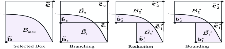
(a) Steps in one iteration

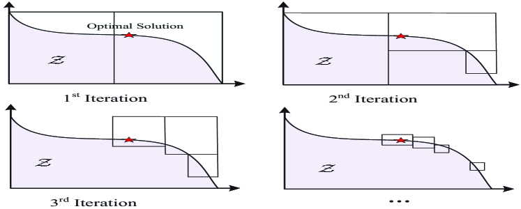
(b) Boxes updating during the iterations

Figure 2: Illustration of the BRB algorithm for MO: the algorithm aims to maximize the objective function by approximating the feasible region using a set of boxes. This approximation process is refined iteratively, with parts that cannot contain the optimal point being removed.

IV-C BRB Algorithm for MO

In this part, we first present the principle of the BRB algorithm to find optimal solutions to the general MO problems in (33). Subsequently, we utilize the BRB algorithm to solve P2a-MO and P2b-MO and illustrate the details using the pseudocode in Algorithm 2. To begin with, we briefly introduce the fundamental principles of solving the general MO problem (33), also illustrated in Fig. 2:

• Since ${\cal L}\left({\bf{z}}\right)$ is monotonically increasing with respect to $\bf z$, the optimal solution must lie on the boundary of the feasible region $\cal Z$. To obtain the optimal solutions, we utilize a box set $\cal N$ associated with multiple non-overlapping boxes to approximate the boundary of the feasible region $\cal Z$, where the optimal solutions are located.

• For one box of the set $\cal N$ denoted by ${\cal B}=\left[{{\bf{b}},{\bf{c}}}\right]$ with lower bound ${f^{\rm lb}\left(\cal B\right)}$ and upper bound ${f^{\rm ub}\left(\cal B\right)}$, we can observe that ${f^{\rm lb}\left(\cal B\right)}={{\cal L}\left({\bf{b}}\right)}$ and $f^{\rm ub}\left(\cal B\right)={{\cal L}\left({\bf{c}}\right)}$, thanks to the monotonically increasing objective function.

• The maximum lower and upper bounds can be found by comparing the lower and upper bounds of all boxes of $\cal N$, and we denote them by $f^{\rm min}_{\cal N}$ and $f^{\rm max}_{\cal N}$, respectively. Then, we iteratively split certain boxes into sub-boxes and try to improve $f^{\rm min}_{\cal N}$ and reduce $f^{\rm max}_{\cal N}$. The algorithm will converge to global optimality with a predefined positive accuracy parameter $\varepsilon$, i.e., $f^{\rm max}_{\cal N}<(1+\varepsilon)f^{\rm min}_{\cal N}$.

Next, we introduce the detailed procedures of the BRB algorithm for solving MO problems. Firstly, we establish an initial box set ${\cal N}=\left\{{\cal B}_{0}\right\}$ where ${\cal B}_{0}=[0,{\bf z}_{0}]$ is the box that contains the whole feasible set $\cal Z$. We initialize the lower and upper bounds by $f^{\rm min}_{\cal N}={\cal L}\left({\bf{0}}\right)=0$ and $f^{\rm max}_{\cal N}={\cal L}\left({\bf{z_{0}}}\right)$. Then, each iteration of the BRB consists of three steps, i.e., branching, reduction, and bounding.

IV-C1 Branching

We first find the specific box ${{\cal B}_{\max}}$ from the box set $\cal N$ that achieves the upper bound $f^{\rm max}_{\cal N}$, i.e.,

$${{\cal B}_{\max}}\buildrel\Delta\over{=}\mathop{\arg\max}\limits_{{\cal B}\in{\cal N}}{f^{{\rm{ub}}}}\left({\cal B}\right).$$ (36)

Then, upon denoting ${{\cal B}_{\max}}=\left[{{\tilde{\bf{b}}},{\tilde{\bf{c}}}}\right]$, we bisect ${{\cal B}_{\max}}$ along its longest side, resulting in two new boxes, i.e.,

$${\tilde{\cal B}_{1}}=\left[{{\tilde{\bf{b}}},{\tilde{\bf{c}}}-\xi{{\bf{e}}_{\dim}}}\right],{\tilde{\cal B}_{2}}=\left[{{\tilde{\bf{b}}}+\xi{{\bf{e}}_{\dim}},{\tilde{\bf{c}}}}\right],$$ (37)

where $\dim=\mathop{\arg\max}\nolimits_{i}\left\{{{{\tilde{c}}_{i}}-{{\tilde{b}}_{i}}}\right\}$ with ${\tilde{c}}_{i}$ and ${\tilde{b}}_{i}$ being the $i$-th element of $\tilde{\bf c}$ and $\tilde{\bf b}$, respectively. Furthermore, $\xi=\frac{{{{\tilde{c}}_{\dim}}-{{\tilde{b}}_{\dim}}}}{2}$ and ${\bf e}_{i}$ is the $i$-th column of ${\bf I}_{K}$. We update the upper bounds of each box as

$${f^{{\rm{ub}}}}\left({{{\tilde{\cal B}}_{1}}}\right) =\min\left\{{{f^{{\rm{ub}}}}\left({\cal B}\right),{\cal L}\left({\tilde{\bf{c}}}-\xi{{\bf{e}}_{\dim}}\right)}\right\},$$ (38a)

$${f^{{\rm{ub}}}}\left({{{\tilde{\cal B}}_{2}}}\right) ={\cal L}\left({\tilde{\bf{c}}}\right).$$ (38b)

IV-C2 Reduction

In this step, we remove parts of the two new boxes that cannot contain the optimal solutions. Specifically, Let the new boxes denoted by ${\tilde{\cal B}_{l}}=\left[{{\bf{\tilde{b}}}_{l},{\bf{\tilde{c}}}}_{l}\right]$ for $l=1,2$. Then, by exploiting monotonicity, we know that ${\tilde{\cal B}_{l}}$ cannot contain the optimal solution and can be removed if it satisfies one of the following constraints:

• ${\bf{\tilde{b}}}_{l}$ is not in the feasible region: because this implies that any vertex $\bf z$ of ${\tilde{\cal B}_{l}}$ satisfies ${\bf{\tilde{b}}}_{l}\leq\bf z$, indicating that it is lies out of the feasible region;

• ${f^{{\rm{ub}}}}\left({\tilde{\cal B}_{l}}\right)\leq f^{\rm min}_{\cal N}$: because this implies that there already exists a feasible solution that is larger than ${\cal L}({\bf z})$ for any vertex $\bf z$ in ${\tilde{\cal B}_{l}}$

On the other hand, if ${f^{{\rm{ub}}}}\left({\tilde{\cal B}_{l}}\right)\geq f^{\rm min}_{\cal N}$, we can also remove redundant vertices of ${\tilde{\cal B}_{l}}$ that cannot be the optimal solution, as illustrated in Fig. 2. Specifically, from [46], we know that the new reduced box ${\tilde{\cal B}}_{l}^{\star}\buildrel\Delta\over{=}\left[{{\bf{\tilde{b}}}_{l}^{\star},{\bf{\tilde{c}}}}_{l}^{\star}\right]$ can contain all the points ${\bf x}\in{\left[{{\bf{\tilde{b}}}_{l},{\bf{\tilde{c}}}}_{l}\right]}$ that satisfy $f^{\rm min}_{\cal N}\leq{\cal L}\left(\bf x\right)\leq{f^{{\rm{ub}}}}\left(\tilde{\cal B}_{l}\right)$, where

$${\bf{\tilde{b}}}_{l}^{\star}={{{\bf{\tilde{c}}}}_{l}}-\sum\nolimits_{k=1}^{K}{\bar{\mu}_{k}}\left({{{\tilde{c}}_{l,k}}-{{\tilde{b}}_{l,k}}}\right){{\bf{e}}_{k}},$$ (39)

$${\bf{\tilde{c}}}_{l}^{\star}={\bf{\tilde{b}}}_{l}^{\star}+\sum\nolimits_{k=1}^{K}{\bar{v}_{k}}\left({{{\tilde{c}}_{l,k}}-\tilde{b}_{l,k}^{\star}}\right){{\bf{e}}_{k}},$$ (40)

with ${\tilde{c}}_{l,k}$, ${\tilde{b}}_{l,k}$, and ${\tilde{b}}_{l,k}^{\star}$ being the $k$-th elements of ${{{\bf{\tilde{c}}}}_{l}}$, ${{{\bf{\tilde{b}}}}_{l}}$, ${{{\bf{\tilde{b}}}}_{l}^{\star}}$, respectively, and $\bar{\mu}_{k}$ and $\bar{v}_{k}$ are given by

$$\!\!{{\bar{\mu}}_{k}} \!=\!\max\!\left\{{\mu\left|\begin{array}[]{l}0\leq\mu\leq 1,\\ {\cal L}\left({{{{\bf{\tilde{c}}}}_{l}}-\mu\left({{{\tilde{c}}_{l,k}}-{{\tilde{b}}_{l,k}}}\right){{\bf{e}}_{k}}}\right)\!\geq\!f_{N}^{\min}\end{array}\right.}\right\},$$ (43)

$$\!\!{{\bar{v}}_{k}} \!=\!\max\!\left\{{v\left|\begin{array}[]{l}0\leq v\leq 1,\\ {\cal L}\left({{\bf{\tilde{b}}}_{l}^{\star}\!+\!v\left({{{\tilde{c}}_{l,k}}-\tilde{b}_{l,k}^{\star}}\right){{\bf{e}}_{k}}}\right)\!\leq\!{f^{{\rm{ub}}}}\left({{{\widetilde{\cal B}}_{l}}}\right)\end{array}\right.}\!\!\!\!\!\right\}.$$ (46)

Note that the closed-form expressions of $\bar{\mu}_{k}$ and $\bar{v}_{k}$ can be obtained in some special cases, e.g., for the weighted sum-rate function with ${\cal L}\left({\bf{z}}\right)=\sum\nolimits_{k=1}^{K}{{\alpha_{k}}{z_{lk}}}$ for $l=1,2$, we have

$$\bar{\mu}_{k} =\min\left\{{1,\frac{{\sum\nolimits_{k=1}^{K}{{\alpha_{k}}{{\tilde{c}}_{l,k}}}-f_{\cal R}^{\min}}}{{{\alpha_{k}}\left({{{\tilde{c}}_{l,k}}-{{\tilde{b}}_{l,k}}}\right)}}}\right\},$$ (47)

$$\bar{v}_{k} =\min\left\{{1,\frac{{{f^{{\rm{ub}}}}\left({\tilde{\cal B}_{l}}\right)-\sum\nolimits_{k=1}^{K}{{\alpha_{k}}{{\tilde{b}}_{l,k}}}}}{{{\alpha_{k}}\left({{{\tilde{c}}_{l,k}}-{{\tilde{b}}_{l,k}}}\right)}}}\right\}.$$ (48)

IV-C3 Bounding

At the end of this iteration, we search for a feasible solution in one of the new boxes ${\tilde{\cal B}}_{l}^{\star}$ and use it for improving $f^{\rm min}_{\cal N}$ and reducing $f^{\rm max}_{\cal N}$. A popular scheme for achieving this is to project the upper vertex of ${\tilde{\cal B}}_{l}^{\star}$ onto the boundary [46]. However, this can potentially increase complexity, since the projection step usually requires a bisection method and each search entails conducting a feasibility check. To reduce the complexity, with the updated box set, ${\cal N}=\left({{\cal N}\backslash{{\cal B}_{\max}}}\right)\cup\left\{{{\tilde{\cal B}_{1}^{\star}},{\tilde{\cal B}_{2}^{\star}}}\right\}$, we just update $f^{\rm min}_{\cal N}$ and $f^{\rm max}_{\cal N}$ as follows:

$$f_{\cal N}^{{\rm{min}}} =\max\left\{{f_{\cal N}^{{\rm{min}}},{\cal L}\left({{\bf{\tilde{b}}}_{2}^{\star}}\right)}\right\},$$ (49)

$$f_{\cal N}^{{\rm{max}}} =\mathop{\arg\max}\limits_{{\cal B}\in{\cal N}}{f^{{\rm{ub}}}}\left({\cal B}\right).$$ (50)

Remark 1

Note that in the reduction step, it is obvious that ${\bf\tilde{b}}_{1}^{\star}$ belongs to the feasible region. However, we must check whether ${\bf\tilde{b}}_{2}^{\star}$ belongs to the feasible region. This also means checking whether we can find the solutions of the remaining optimization variables in problems P2a-MO or P2b-MO to make them feasible when ${\bf z}={\bf\tilde{b}}_{2}^{\star}$. Specifically, when using the BRB to solve problem P2a-MO, the corresponding feasibility check problem is given by

$${\rm find}\;{\bf p}$$ (P2a-F)

$${\rm s.t.} \;\frac{{{2^{z_{qib}^{{\rm N},q}}}-1}}{{{\gamma_{qqb}}}}\leq{p_{qb}},$$

$$\frac{{\left({{2^{z_{qib}^{{\rm N},i}}}-1}\right)\left({{\gamma_{iqb}}{p_{qb}}+1}\right)}}{{{\gamma_{iib}}}}\leq{p_{ib}},\forall b\in{{\cal R}_{r}},\eqref{eq31},$$

As for problem P2b-MO, the corresponding feasibility check problem is given by

$${\rm{find}}\;{\bf{p}}$$ (P2b-F)

$${\rm{s}}.{\rm{t}}. \;\frac{{\left({{2^{z_{qb}^{\rm{S}}}}-1}\right)\left({\sum\nolimits_{i\neq q}^{Q}{{\gamma_{qib}}{p_{ib}}}+1}\right)}}{{{\gamma_{qqb}}}}\leq{p_{qb}},\forall b\in{{\cal R}_{r}},\eqref{eq32}.$$

Since the constraints are affine functions and ${z_{qib}^{{\rm N},q}}$, ${z_{qib}^{{\rm N},i}}$, and ${z_{qb}^{\rm{S}}}$ are constant parameters based on the lower vertex of the corresponding box, the above two problems are convex optimization problems. Thus, they can be efficiently solved by using the Matlab toolbox CVX [47].

Finally, the details of applying BRB to solve the MO problem are summarized in Algorithm 1. Note that although this algorithm can obtain the $\varepsilon$-accuracy globally optimal solution at a lower complexity than the exhaustive search, the DPMO algorithm still imposes exponentially increasing complexity and cannot be applied to the general case involving rate constraints.

Algorithm 2 Optimal solutions to P2a-MO (or P2b-MO)

1:  Initialize ${\cal B}_{0}=\left[{\bf 0},{\bf z}_{0}\right]$, where the elements of ${\bf z}_{0}$ are set as $z_{qib}^{{\rm N},q}={\log_{2}}\left({1+{\gamma_{qqb}}{p_{r}}}\right)$,$z_{qib}^{{\rm N},i}={\log_{2}}\left({1+{\gamma_{iib}}{p_{r}}}\right)$ for problem P2b-MO (or $z_{qb}^{{\rm S}}={\log_{2}}\left({1+{\gamma_{qqb}}{p_{r}}}\right)$ for problem P2b-MO)

2:  Set ${\cal N}=\left\{{\cal B}_{0}\right\}$, and $f^{\rm min}_{\cal N}={\cal L}^{\rm X}\left({\bf{0}}\right)=0$ and $f^{\rm max}_{\cal N}={\cal L}^{\rm X}\left({\bf{z}}_{0}\right)$ where “${\rm X}={\rm N}$” for P2a-MO and “${\rm X}={\rm S}$” for P2b-MO

3:  while $f^{\rm max}_{\cal N}>(1+\varepsilon)f^{\rm min}_{\cal N}$ and below the maximum number of iterations do

4:     Find ${{\cal B}_{\max}}$ by (36)

5:     for $l=1,2$ do

6:        Create new box ${{\tilde{\cal B}}_{l}}$ by (37); Set ${f^{{\rm{ub}}}}\left({{{\tilde{\cal B}}_{l}}}\right)$ by (38)

7:        if $f^{\rm min}_{\cal N}\leq{f^{{\rm{ub}}}}\left({{{\tilde{\cal B}}_{l}}}\right)$:     Calculate ${{\tilde{\cal B}}_{l}^{\star}}$ by utilizing (39) and (40) for ${{\tilde{\cal B}}_{l}}$; else: set ${{\tilde{\cal B}}_{l}^{\star}}=\emptyset$ end if

8:     end for

9:     Check feasibility of ${\bf{\tilde{b}}}_{2}^{\star}$ by solving P2a-F for P2a-MO (or by solving P2b-F for P2b-MO)

10:     if feasible:     Update the lower bound $f^{\rm min}_{\cal N}$ by (49); else: set ${{\tilde{\cal B}}_{2}^{\star}}=\emptyset$ end if

11:     Update box set ${\cal N}=\left({{\cal N}\backslash{{\cal B}_{\max}}}\right)\cup\left\{{{\tilde{\cal B}_{1}^{\star}},{\tilde{\cal B}_{2}^{\star}}}\right\}$

12:     Update the upper bound $f^{\rm max}_{\cal N}$ by (50)

13:  end while

14:  Return a feasible solution that can achieve $f^{\rm min}_{\cal N}$.

V Suboptimal Solution to The General Case: With Rate Constraints

The DPMO method solves problem P1 in the special scenario of no rate constraints, and it exhibits exponential complexity. To efficiently solve it for the general cases with rate constraints, we employ the SCA-SA algorithm to find the sub-optimal solution within polynomial time complexity.

V-A Simulated Annealing (SA) Algorithm Development

In the face of individual rate constraints, the original problem P1 is hard to solve and cannot be directly divided into independent problems using the DP framework. Therefore, we need to develop efficient sub-optimal algorithms.

To begin with, we need to decouple the optimization of the binary variables ${\bf a}^{\rm S}$ and ${\bf a}^{\rm N}$. To do so, we first apply the SA algorithm [48] to find the sub-optimal solution of ${\bf{P1}}$ by randomly setting ${\bf a}^{\rm S}$ iteratively. Specifically, we denote the randomly selected solution of ${\bf a}^{\rm S}$ and the corresponding objective function value in the $t$-th iteration of SA by ${\bf a}^{\rm S}_{t}$ and $\tilde{C}\left({{\bf{a}}_{t}^{\rm{S}}}\right)$, respectively. Besides, $\tilde{C}\left({{\bf{a}}_{t}^{\rm{S}}}\right)$ is obtained by solving ${\bf{P1}}$ with ${{\bf{a}}^{\rm{S}}}={\bf{a}}_{t}^{\rm{S}}$, i.e.,

$${{\tilde{C}}}\left({{\bf{a}}_{t}^{\rm{S}}}\right)\buildrel\Delta\over{=}\mathop{\max}\limits_{{{\bf{a}}^{\rm{S}}}={\bf{a}}_{t}^{\rm{S}},{{\bf{a}}^{\rm{N}}},{\bf{p}}} \sum\nolimits_{r=1}^{R}{{C_{r}}}$$ (P3)

$${\rm{s}}.{\rm{t}}.\quad \eqref{eqP1a0}-\eqref{eqP1c}.$$

The suboptimal solution to P3 can be obtained by applying SCA algorithm, which will be discussed in Section V-B.

After solving problem P3, the current optimum user accommodation and access scheme of ${\bf a}^{\rm S}$ can be replaced as follows:

$${\bf{a}}_{\star}^{\rm S}\leftarrow\left\{{\begin{array}[]{*{20}{l}}{{\bf{a}}_{t}^{\rm{S}},\;{\rm{if}}\;{{\bar{C}}^{\star}}\leq{{\tilde{C}}}\left({{\bf{a}}_{t}^{\rm{S}}}\right),}\\ {{\bf{a}}_{\star}^{\rm S},{\rm{otherwise}}},\end{array}}\right.$$ (53)

where ${\bf a}_{\star}^{\rm S}$ is the current optimal solution of ${\bf a}^{\rm S}$ that can achieve the maximum objective value ${{\bar{C}}^{\star}}$ in the previous iterations of SA, i.e., ${\bar{C}^{\star}}=\mathop{\max}\nolimits_{0\leq i\leq t-1}\tilde{C}\left({{\bf{a}}_{i}^{\rm{S}}}\right)$.

Then, to search for potential better solutions, we further explore other solutions of ${\bf a}^{\rm S}$. To do so, we denote an integer index $x$, which is randomly uniformly generated from the set $\left\{{1,2,\cdots,R}\right\}$. Consequently, we update ${\bf{a}}^{\rm{S}}$ in the $(t+1)$-th iteration as follows:

$${\left[{{\bf{a}}_{t+1}^{\rm{S}}}\right]_{r}}=\left\{{\begin{array}[]{*{20}{l}}{{{\left[{{\bf{\tilde{a}}}_{t}^{\rm{S}}}\right]}_{r}},\;{\rm{if}}\;r\neq x,}\\ {1-{{\left[{{\bf{\tilde{a}}}_{t}^{\rm{S}}}\right]}_{r}},{\rm{if}}\;r=x,}\end{array}}\right.$$ (56)

for $1\leq r\leq R$, where ${{{\left[{{\bf{a}}_{t+1}^{\rm{S}}}\right]}_{r}}}$ and ${{{\left[{{\bf{\tilde{a}}}_{t}^{\rm{S}}}\right]}_{r}}}$ are the $r$-th elements of vectors ${\bf{a}}_{t+1}^{\rm{S}}$ and ${\bf{\tilde{a}}}_{t}^{\rm{S}}$, respectively. Besides, ${\bf{\tilde{a}}}_{t}^{\rm{S}}$ is the solution updated by comparing ${{\bar{C}}^{\star}}$ and ${{\tilde{C}}}\left({{\bf{a}}_{t}^{\rm{S}}}\right)$, i.e.,

$${\bf{\tilde{a}}}_{t}^{\rm{S}}=\left\{{\begin{array}[]{*{20}{l}}{{\bf{a}}_{t}^{\rm{S}},\;{\rm{if}}\;{{\bar{C}}^{\star}}\leq\tilde{C}\left({{\bf{a}}_{t}^{\rm{S}}}\right),}\\ {{\bf{\hat{a}}}_{t}^{\rm{S}},\;{\rm{if}}\;{{\bar{C}}^{\star}}>\tilde{C}\left({{\bf{a}}_{t}^{\rm{S}}}\right),}\end{array}}\right.$$ (59)

where ${\bf{\hat{a}}}_{t}^{\rm{S}}=\left\{{\begin{array}[]{*{20}{l}}{{\bf{a}}_{t}^{\rm{S}},{\rm{with}}\;{\rm{probability}}\;{\cal P}_{t}}\\ {{\bf{\tilde{a}}}_{\star}^{\rm{S}}{\rm{,{\rm{with}}\;{\rm{probability}}\;(1-{\cal P}_{t})}}}\end{array}}\right.$. Here, we define the probability by ${\cal P}_{t}=\exp\left({\frac{1}{{T_{e}^{t}}}\left({{{\tilde{C}}}\left({{\bf{a}}_{t}^{\rm{S}}}\right)-{{\bar{C}}^{\star}}}\right)}\right)$, where $T_{e}^{t}$ is the temperature in $t$-th iteration of the SA algorithm, which will be updated by $T_{e}^{t+1}={\bar{\zeta}}T_{e}^{t}$. The parameter $0<{\bar{\zeta}}<1$ is the cooling factor, which determines how the temperature gradually decreases throughout the iterations, influencing the exploration and convergence speed in the search space. In this way, it allows the selected suboptimal ${\bf a}^{\rm S}$ a chance to enable the SA algorithm to escape poor local optima and converge to better solutions. Note that to reduce the computational complexity, if the randomly generated index $x$ results in ${\bf{a}}_{t+1}^{\rm{S}}$ that has already appeared, we have to regenerate this index so that the resultant ${\bf{a}}_{t+1}^{\rm{S}}$ is unprecedented.

It is readily apparent that the utility will not decrease during each iteration. Furthermore, the convergence can be guaranteed because the probability ${\cal P}_{t}$ decreases as the temperature decreases. Finally, the details are summarized in Algorithm 3.

V-B Sub-Optimal Solution of Problem P3

During each iteration of SA, we have to solve problem P3. However, this problem is hard to solve due to the remaining binary variables ${\bf a}^{\rm N}$. In the following, we transform problem P3 into a solvable form by introducing additional auxiliary and some necessary approximations and then apply the SCA algorithm to solve it efficiently.

Firstly, we introduce the auxiliary optimization variables $\bf\tilde{p}$, whose elements include $\left\{{\tilde{p}_{qib}^{{\rm{N}},q},\tilde{p}_{qib}^{{\rm{N}},i}\left|{\forall b,\forall\left({q,i}\right)\in{\cal Q}}\right.}\right\}$ and $\left\{{\tilde{p}_{qb}^{\rm{S}}\left|{\forall b,\forall q}\right.}\right\}$. Here, we define $\tilde{p}_{qib}^{{\rm{N}},q}=a_{rqi}^{\rm{N}}{p_{qb}}$ and $\tilde{p}_{qib}^{{\rm{N}},i}=a_{rqi}^{\rm{N}}{p_{ib}}$ if $b\in{\cal R}_{r}$, and $\tilde{p}_{qb}^{\rm{S}}={{{\left[{{\bf{\tilde{a}}}_{t}^{\rm{S}}}\right]}_{r}}}{p_{qb}}$ if $b\in{\cal R}_{r}$. Since some of the multiplicative terms consist of binary variables $a_{rqi}^{\rm{N}}$, problem P3 is challenging to solve. We apply the big-M method to decompose them [32], yielding:

$$\tilde{p}_{qib}^{{\rm{N}},q}\leq{p_{qb}},\tilde{p}_{qib}^{{\rm{N}},q}\geq{p_{qb}}-\left({1-a_{rqi}^{\rm{N}}}\right)P,\tilde{p}_{qib}^{{\rm{N}},q}\geq 0,$$

$$\qquad\qquad\qquad\qquad\quad\forall b\in{{\cal R}_{r}},\forall r,\forall\left({q,i}\right)\in{\cal Q},$$ (60)

$$\tilde{p}_{qib}^{{\rm{N}},i}\leq{p_{ib}},\tilde{p}_{qib}^{{\rm{N}},i}\geq{p_{ib}}-\left({1-a_{rqi}^{\rm{N}}}\right)P,\tilde{p}_{qib}^{{\rm{N}},i}\geq 0,$$

$$\qquad\qquad\qquad\qquad\quad\forall b\in{{\cal R}_{r}},\forall r,\forall\left({q,i}\right)\in{\cal Q}.$$ (61)

Algorithm 3 SCA-SA algorithm to solve P1

1:  Initialize ${\bf{a}}_{\star}^{\rm S}={\bf 1}_{R}$; initialize ${{\bar{C}}^{\star}}=\tilde{C}\left({\bf{a}}_{\star}^{\rm S}\right)$ by using SCA to solve problem P3; initialize $t=0$, ${\bf{a}}_{t}^{\rm S}={\bf 0}_{R}$, ${\bar{\zeta}}=0.92$, $T_{e}^{t}=\max\left\{{{{\bar{C}}^{\star}},10}\right\}$

2:  repeat

3:     $t\leftarrow t+1$ and calculate ${{\tilde{C}}}\left({{\bf{a}}_{t}^{\rm{S}}}\right)$ by using SCA algorithm to solve P3 (i.e., solve P3-2 iteratively)

4:     Update ${\bf{a}}_{\star}^{\rm S}$ by (53); Update ${\bf{a}}_{t+1}^{\rm{S}}$ by (56); Update ${{\bar{C}}^{\star}}=\max\left\{{{{\bar{C}}^{\star}},\tilde{C}\left({{\bf{a}}_{t}^{\rm{S}}}\right)}\right\}$ and $T_{e}^{t+1}={\bar{\zeta}}T_{e}^{t}$

5:  until Convergence

6:  Return the solutions of ${{\bf{a}}^{\rm{S}}}$, ${{\bf{a}}^{\rm{N}}}$, and ${\bf{p}}$.

Based on these auxiliary variables and the average rate defined in (23) and (25), we have

$$\tilde{C}_{rqi}^{{\rm{N}},q} \buildrel\Delta\over{=}a_{rqi}^{\rm{N}}C_{rqi}^{{\rm{N}},q}=\frac{1}{{MN}}\sum\limits_{b\in{{\cal R}_{r}}}{{{\log}_{2}}\left({1+{\gamma_{qqb}}\tilde{p}_{qib}^{{\rm{N}},q}}\right)},$$ (62)

$$\tilde{C}_{rqi}^{{\rm{N}},i} \buildrel\Delta\over{=}a_{rqi}^{\rm{N}}C_{rqi}^{{\rm{N}},i}=\frac{1}{{MN}}\sum\limits_{b\in{{\cal R}_{r}}}{{{\log}_{2}}\left({1+\nu_{qib}^{{\rm{N}}}}\right)},$$ (63)

$$\tilde{C}_{rq}^{\rm{S}} \buildrel\Delta\over{=}a_{t,r}^{\rm{S}}C_{rq}^{\rm{S}}=\frac{1}{{MN}}\sum\limits_{b\in{{\cal R}_{r}}}{{{\log}_{2}}\left({1+\nu_{qb}^{\rm{S}}}\right)},$$ (64)

where $\nu_{qib}^{{\rm{N}}}=\frac{{{\gamma_{iib}}\tilde{p}_{qib}^{{\rm{N}},i}}}{{{\gamma_{iqb}}\tilde{p}_{qib}^{{\rm{N}},q}}+1}$ for $b\in{\cal R}_{r},\forall r,\forall\left({q,i}\right)\in{\cal Q}$ and $\nu_{qb}^{\rm{S}}=\frac{{{\gamma_{qqb}}\tilde{p}_{qb}^{\rm{S}}}}{{\sum\nolimits_{i\neq q}{{\gamma_{qib}}\tilde{p}_{ib}^{\rm{S}}}+1}}$ for $b\in{\cal R}_{r},\forall r,\forall q$.

By substituting them into problem P3, the objective function and the achievable transmission rate of the $q$-th user defined in the individual rate constraint (27a) can be reformulated as:

$$\tilde{C}\left({{\bf{\tilde{p}}},{\mbox{\boldmath{$\nu$}}}}\right) =\sum\limits_{r=1}^{R}{{C_{r}}}$$

$$=\sum\limits_{q=1}^{Q-1}{\sum\limits_{i=q+1}^{Q}{\left({{\alpha_{q}}\tilde{C}_{rqi}^{{\rm{N}},q}+{\alpha_{i}}\tilde{C}_{rqi}^{{\rm{N}},i}}\right)}}+\sum\limits_{q=1}^{Q}{{\alpha_{q}}\tilde{C}_{rq}^{\rm{S}}},$$ (65)

$${{\tilde{C}}_{q}}\left({{\bf{\tilde{p}}},{\mbox{\boldmath{$\nu$}}}}\right) =\sum\limits_{r=1}^{R}{\left({\sum\limits_{i=1}^{q-1}{\tilde{C}_{riq}^{{\rm{N}},q}}+\sum\limits_{i=q+1}^{Q}{\tilde{C}_{rqi}^{{\rm{N}},q}+}\tilde{C}_{rq}^{\rm{S}}}\right)},$$ (66)

where $\nu$ is a vector consisting of these elements $\left\{{\nu_{qib}^{\rm{N}}\left|{\forall b\in{{\cal R}_{r}},\forall r,\forall\left({q,i}\right)\in{\cal Q}}\right.}\right\}$ and $\left\{{\nu_{qb}^{\rm{S}}\left|{\forall b\in{{\cal R}_{r}},\forall r,\forall q}\right.}\right\}$. Due to the existence of the individual QoS constraint, we introduce the following constraints to guarantee that each user can gain access at least once for information transmission if ${C_{\min,q}}>0$, i.e.,

$$\sum\nolimits_{r=1}^{R}{\left({\sum\nolimits_{i=1}^{q-1}{a_{riq}^{\rm{N}}+\sum\nolimits_{i=q+1}^{Q}{a_{rqi}^{\rm{N}}+a_{t,r}^{\rm{S}}}}}\right)}\geq{{\rm{I}}_{q}},$$ (67)

where ${{\rm{I}}_{q}}=\left\{0,1\right\}$ is a constant dependent on the minimal QoS requirement, i.e., ${{\rm{I}}_{q}}=1$ if ${C_{\min,q}}>0$, otherwise ${{\rm{I}}_{q}}=0$.

To address the binary integer constraint (27f) in P3, we introduce the following joint continuous equivalent constraints to replace it:

$$0\leq a_{rqi}^{\rm{N}}\leq 1,0\leq a_{r}^{\rm{N}}\leq 1,\forall r,\forall\left({q,i}\right)\in{\cal Q},$$ (68)

$${\sum\nolimits_{r=1}^{R}{\sum\nolimits_{q=1}^{Q-1}{\sum\nolimits_{i=q+1}^{Q}{\left({a_{rqi}^{\rm{N}}-{{\left({a_{rqi}^{\rm{N}}}\right)}^{2}}}\right)}}}}\leq 0.$$ (69)

With the above constraints (68) and (69), the binary variables $a_{rqi}^{\rm{N}}$ have been converted into continuous optimization variables. Although there are only continuous constraints and no direct integer constraints (27f), the joint constraints (54) and (55) effectively restrict the solution to integer values. Thus, this step is an equivalent substitution.

However, constraint (69) is non-convex, which still makes P3 hard to solve. Therefore, we introduce a penalty factor $\eta$ to relax (69) in the objective function. By further combining it with the above additional constraints and variables, we can reformulate problem P3 into the following form:

$$\mathop{\max}\limits_{{{\bf{a}}^{\rm{N}}},{\bf{p}},{\bf{\tilde{p}}},{\mbox{\boldmath{$\nu$}}}} \tilde{C}\left({\bf{\tilde{p}}},{\mbox{\boldmath{$\nu$}}}\right)+\eta\left({\tilde{G}\left({{{\bf{a}}^{N}}}\right)-G\left({{{\bf{a}}^{N}}}\right)}\right)$$ (P3-1)

$${\rm{s}}{\rm{.t}}{\rm{.}}\; \tilde{C}_{q}{\left({\bf{\tilde{p}}},{\mbox{\boldmath{$\nu$}}}\right)}\geq{C_{\min,q}},\forall q,$$ (70a)

$$V_{qib}^{\rm{N}}\left({{\bf{\tilde{p}}},{\mbox{\boldmath{$\nu$}}}}\right)-\tilde{V}_{qib}^{\rm{N}}\left({{\bf{\tilde{p}}},{\mbox{\boldmath{$\nu$}}}}\right)\leq{\gamma_{iib}}\tilde{p}_{qib}^{{\rm{N}},i},$$

$$\qquad\qquad\qquad\qquad\forall b\in{{\cal R}_{r}},\forall r,\forall\left({q,i}\right)\in{\cal Q},$$ (70b)

$${\gamma_{qqb}}\tilde{p}_{rqi}^{{\rm{N,}}q}-{\gamma_{qib}}\tilde{p}_{rqi}^{{\rm{N,}}i}\leq 0,$$

$$\qquad\qquad\qquad\qquad\forall b\in{{\cal R}_{r}},\forall r,\forall\left({q,i}\right)\in{\cal Q},$$ (70c)

$$V_{qb}^{\rm{S}}\left({{\bf{\tilde{p}}},{\mbox{\boldmath{$\nu$}}}}\right)-\tilde{V}_{qb}^{\rm{S}}\left({{\bf{\tilde{p}}},{\mbox{\boldmath{$\nu$}}}}\right)\leq{\gamma_{qqb}}\tilde{p}_{qb}^{\rm{S}},$$

$$\qquad\qquad\qquad\qquad\qquad\qquad\forall b\in{{\cal R}_{r}},\forall r,\forall q,$$ (70d)

$$\eqref{eqP1b0},\eqref{eqP1d},\eqref{eqintegerr1}-\eqref{eqintegerr2},\eqref{eqc61},\eqref{eqAapproximate1},$$

where the factor $\eta$, which should be much larger than 1 [32, 49], is used to penalize the objective function in cases where $a_{rqi}^{\rm N}$ is neither 0 nor 1; (70c) is due to (27d); and

$$G\left({{{\bf{a}}^{N}}}\right)=\sum\nolimits_{r=1}^{R}{\sum\nolimits_{q=1}^{Q-1}{\sum\nolimits_{i=q+1}^{Q}{a_{rqi}^{\rm{N}}}}},$$ (71)

$$\tilde{G}\left({{{\bf{a}}^{N}}}\right)=\sum\nolimits_{r=1}^{R}{\sum\nolimits_{q=1}^{Q-1}{\sum\nolimits_{i=q+1}^{Q}{{{\left({a_{rqi}^{\rm{N}}}\right)}^{2}}}}},$$ (72)

$$V_{qib}^{\rm{N}}\left({{\bf{\tilde{p}}},{\mbox{\boldmath{$\nu$}}}}\right)={\left({\nu_{qib}^{\rm{N}}+{\gamma_{iqb}}\tilde{p}_{qib}^{{\rm{N}},q}+1}\right)^{2}},$$ (73)

$$\tilde{V}_{qib}^{\rm{N}}\left({{\bf{\tilde{p}}},{\mbox{\boldmath{$\nu$}}}}\right)={\left({\nu_{qib}^{\rm{N}}-{\gamma_{iqb}}\tilde{p}_{qib}^{{\rm{N}},q}-1}\right)^{2}},$$ (74)

$$V_{qb}^{\rm{S}}\left({{\bf{\tilde{p}}},{\mbox{\boldmath{$\nu$}}}}\right)={\left({\nu_{qb}^{\rm{S}}+\sum\nolimits_{i\neq q}{{\gamma_{qib}}\tilde{p}_{ib}^{\rm{S}}}+1}\right)^{2}},$$ (75)

$$\tilde{V}_{qb}^{\rm{S}}\left({{\bf{\tilde{p}}},{\mbox{\boldmath{$\nu$}}}}\right)={\left({\nu_{qb}^{\rm{S}}-\sum\nolimits_{i\neq q}{{\gamma_{qib}}\tilde{p}_{ib}^{\rm{S}}}-1}\right)^{2}}.$$ (76)

It is obvious that $\tilde{C}\left({{\bf{\tilde{p}}},{\mbox{\boldmath{$\nu$}}}}\right)$, ${{\tilde{C}}_{q}}\left({{\bf{\tilde{p}}},{\mbox{\boldmath{$\nu$}}}}\right)$, $G\left({{{\bf{a}}^{N}}}\right)$, $\tilde{G}\left({{{\bf{a}}^{N}}}\right)$, $V_{qib}^{{\rm{N}},i}\left({{\bf{\tilde{p}}},{\mbox{\boldmath{$\nu$}}}}\right)$, $\tilde{V}_{qib}^{{\rm{N}},i}\left({{\bf{\tilde{p}}},{\mbox{\boldmath{$\nu$}}}}\right)$, $V_{qb}^{\rm{S}}\left({{\bf{\tilde{p}}},{\mbox{\boldmath{$\nu$}}}}\right)$, and $\tilde{V}_{qb}^{\rm{S}}\left({{\bf{\tilde{p}}},{\mbox{\boldmath{$\nu$}}}}\right)$ are affine or convex functions. Thus, problem P3-1 belongs to the standard difference of convex (DC) family [50], where the objective function or constraints can be expressed in terms of the differences between two concave/convex functions. Hence, we can apply the SCA method to solve it iteratively. In each iteration, the Taylor series expansion is used for approximating the convex/concave terms by linear functions, thus transforming them into convex problems. Specifically, defining the solutions of ${{\bf{a}}^{\rm{N}}}$, ${\bf{\tilde{p}}}$, $\nu$ in the $(i-1)$-th iteration by ${\bf{a}}^{\rm{N}}_{\imath}$, ${\bf{\tilde{p}}}_{\imath}$, ${\mbox{\boldmath{$\nu$}}}_{\imath}$, we have

$$\tilde{G}\left({{{\bf{a}}^{\rm{N}}}}\right) \mathop{\geq}\limits_{\left(\rm a\right)}\tilde{G}\left({{\bf{a}}_{\imath}^{\rm{N}}}\right)+\nabla\tilde{G}{\left({{\bf{a}}_{\imath}^{\rm{N}}}\right)^{T}}\left({{{\bf{a}}^{\rm{N}}}-{\bf{a}}_{\imath}^{\rm{N}}}\right)$$

$$\buildrel\Delta\over{=}{{\tilde{G}}^{{\rm{lb}}}}\left({{{\bf{a}}^{\rm{N}}};{\bf{a}}_{\imath}^{\rm{N}}}\right),$$ (77)

$$\tilde{V}_{qib}^{{\rm{N}}}\left({{\bf{\tilde{p}}},{\mbox{\boldmath{$\nu$}}}}\right){\rm{}} \mathop{\geq}\limits_{\left({\rm{b}}\right)}\tilde{V}_{qib}^{{\rm{N}}}\left({{\bf{\tilde{p}}},{\mbox{\boldmath{$\nu$}}}}\right)+{\left[{\begin{array}[]{*{20}{c}}{\nabla V_{qib}^{{\rm{N}}}\left({{{{\bf{\tilde{p}}}}_{\imath}}}\right)}\\ {\nabla V_{qib}^{{\rm{N}}}\left({{{\mbox{\boldmath{$\nu$}}}_{\imath}}}\right)}\end{array}}\right]^{T}}\left[{\begin{array}[]{*{20}{c}}{{\bf{\tilde{p}}}-{{{\bf{\tilde{p}}}}_{\imath}}}\\ {{\mbox{\boldmath{$\nu$}}}-{{\mbox{\boldmath{$\nu$}}}_{\imath}}}\end{array}}\right]$$ (82)

$$\buildrel\Delta\over{=}\tilde{V}_{qib}^{{\rm{lb}},{\rm{N}}}\left({{\bf{\tilde{p}}},{\mbox{\boldmath{$\nu$}}};{{{\bf{\tilde{p}}}}_{\imath}},{{\mbox{\boldmath{$\nu$}}}_{\imath}}}\right),$$ (83)

$$\tilde{V}_{qb}^{\rm{S}}\left({{\bf{\tilde{p}}},{\mbox{\boldmath{$\nu$}}}}\right) \mathop{\geq}\limits_{\left({\rm{c}}\right)}\tilde{V}_{qb}^{\rm{S}}\left({{\bf{\tilde{p}}},{\mbox{\boldmath{$\nu$}}}}\right)+{\left[{\begin{array}[]{*{20}{c}}{\nabla V_{qb}^{\rm{S}}\left({{{{\bf{\tilde{p}}}}_{\imath}}}\right)}\\ {\nabla V_{qb}^{\rm{S}}\left({{{\mbox{\boldmath{$\nu$}}}_{\imath}}}\right)}\end{array}}\right]^{T}}\left[{\begin{array}[]{*{20}{c}}{{\bf{\tilde{p}}}-{{{\bf{\tilde{p}}}}_{\imath}}}\\ {{\mbox{\boldmath{$\nu$}}}-{{\mbox{\boldmath{$\nu$}}}_{\imath}}}\end{array}}\right]$$ (88)

$$\buildrel\Delta\over{=}\tilde{V}_{qb}^{{\rm{lb}},{\rm{S}}}\left({{\bf{\tilde{p}}},{\mbox{\boldmath{$\nu$}}};{{{\bf{\tilde{p}}}}_{\imath}},{{\mbox{\boldmath{$\nu$}}}_{\imath}}}\right),$$ (89)

where $\nabla\tilde{G}\left({{\bf{a}}_{\imath}^{\rm{N}}}\right)=\frac{{\partial\tilde{G}\left({{{\bf{a}}^{\rm{N}}}}\right)}}{{\partial{{\bf{a}}^{\rm{N}}}}}\left|{{}_{{{\bf{a}}^{\rm{N}}}={\bf{a}}_{\imath}^{\rm{N}}}}\right.$, $\nabla V_{qib}^{{\rm{N}},i}\left({{{{\bf{\tilde{p}}}}_{\imath}}}\right)=\frac{{\partial\tilde{V}_{qib}^{{\rm{N}},i}\left({{\bf{\tilde{p}}},{\mbox{\boldmath{$\nu$}}}}\right)}}{{\partial{\bf{\tilde{p}}}}}\left|{{}_{{\bf{\tilde{p}}}={{{\bf{\tilde{p}}}}_{\imath}},{\mbox{\boldmath{$\nu$}}}={{\mbox{\boldmath{$\nu$}}}_{\imath}}}}\right.$, $\nabla V_{qib}^{{\rm{N}},i}\left({{{\mbox{\boldmath{$\nu$}}}_{\imath}}}\right)=\frac{{\partial\tilde{V}_{qib}^{{\rm{N}},i}\left({{\bf{\tilde{p}}},{\mbox{\boldmath{$\nu$}}}}\right)}}{{\partial{\mbox{\boldmath{$\nu$}}}}}\left|{{}_{{\bf{\tilde{p}}}={{{\bf{\tilde{p}}}}_{\imath}},{\mbox{\boldmath{$\nu$}}}={{\mbox{\boldmath{$\nu$}}}_{\imath}}}}\right.$, $\nabla V_{qb}^{\rm{S}}\left({{{{\bf{\tilde{p}}}}_{\imath}}}\right)=\frac{{\partial\tilde{V}_{qb}^{\rm{S}}\left({{\bf{\tilde{p}}},{\mbox{\boldmath{$\nu$}}}}\right)}}{{\partial{\bf{\tilde{p}}}}}\left|{{}_{{\bf{\tilde{p}}}={{{\bf{\tilde{p}}}}_{\imath}},{\mbox{\boldmath{$\nu$}}}={{\mbox{\boldmath{$\nu$}}}_{\imath}}}}\right.$, and $\nabla V_{qb}^{\rm{S}}\left({{{\mbox{\boldmath{$\nu$}}}_{\imath}}}\right)=\frac{{\partial\tilde{V}_{qb}^{\rm{S}}\left({{\bf{\tilde{p}}},{\mbox{\boldmath{$\nu$}}}}\right)}}{{\partial{\mbox{\boldmath{$\nu$}}}}}\left|{{}_{{\bf{\tilde{p}}}={{{\bf{\tilde{p}}}}_{\imath}},{\mbox{\boldmath{$\nu$}}}={{\mbox{\boldmath{$\nu$}}}_{\imath}}}}\right.$ are constant gradients of the functions $\tilde{G}\left({{{\bf{a}}^{\rm{N}}}}\right)$, $\tilde{V}_{qib}^{{\rm{N}},i}\left({{\bf{\tilde{p}}},{\mbox{\boldmath{$\nu$}}}}\right)$, and $\tilde{V}_{qb}^{\rm{S}}\left({{\bf{\tilde{p}}},{\mbox{\boldmath{$\nu$}}}}\right)$ with respect to $\bf a$, $\tilde{\bf p}$, and $\nu$, respectively. Here, the inequalities at (a) in (77), (b) in (83), and (c) in (89), are due to the semidefinite Hessian matrix of the concave function, which makes the right-hand side lower than the left-hand side [50].

Therefore, by harnessing the lower bounds defined in (77), (83), and (89), problem P3-1 can be solved by iteratively solving the following problem

$$\mathop{\max}\limits_{{{\bf{a}}^{\rm{N}}},{\bf{p}},{\bf{\tilde{p}}},{\mbox{\boldmath{$\nu$}}}} C\left({{\bf{\tilde{p}}},{\mbox{\boldmath{$\nu$}}}}\right)+\eta\left({{{\tilde{G}}^{{\rm{lb}}}}\left({{{\bf{a}}^{\rm{N}}};{\bf{a}}_{\imath}^{\rm{N}}}\right)-G\left({{{\bf{a}}^{N}}}\right)}\right)$$ (P3-2)

$${\rm{s}}.{\rm{t}}.\; V_{iqb}^{\rm{N}}\left({{\bf{\tilde{p}}},{\mbox{\boldmath{$\nu$}}}}\right)-\tilde{V}_{qb}^{{\rm{lb}},{\rm{N}}}\left({{\bf{\tilde{p}}},{\mbox{\boldmath{$\nu$}}};{{{\bf{\tilde{p}}}}_{\imath}},{{\mbox{\boldmath{$\nu$}}}_{\imath}}}\right)\leq{\gamma_{qqb}}\tilde{p}_{iqb}^{{\rm{N}},q},$$

$$\qquad\qquad\qquad\forall b\in{{\cal R}_{r}},\forall r,\forall\left({q,i}\right)\in{\cal Q},$$ (90a)

$$V_{qb}^{\rm{S}}\left({{\bf{\tilde{p}}},{\mbox{\boldmath{$\nu$}}}}\right)-\tilde{V}_{qb}^{{\rm{lb}},{\rm{S}}}\left({{\bf{\tilde{p}}},{\mbox{\boldmath{$\nu$}}};{{{\bf{\tilde{p}}}}_{\imath}},{{\mbox{\boldmath{$\nu$}}}_{\imath}}}\right)\leq{\gamma_{qqb}}\tilde{p}_{qb}^{\rm{S}},$$

$$\qquad\qquad\qquad\qquad\qquad\forall b\in{{\cal R}_{r}},\forall r,q,$$ (90b)

$$\eqref{eqP1b0},\eqref{eqP1d},\eqref{eqintegerr1}-\eqref{eqintegerr2},\eqref{eqc61},\eqref{eqAapproximate1},\eqref{eq56a},\eqref{eq56d}.$$

Obviously, problem P3-2 is convex due to the concave objective function and convex constraints. Therefore, it can be solved optimally by using the Matlab toolbox CVX. Then, we repeat this approximation and the convergence can be guaranteed due to the iteratively increased objective function.

In summary, problem P3 is relaxed as P3-1, whose approximated solution can be obtained by solving P3-2 iteratively.

V-C Complexity Analysis

In this subsection, we analyze the complexity of the proposed sub-optimal Algorithm 3, which consists of an inner loop for the SCA algorithm and an outer loop for the SA algorithm. The primary computational complexity arises from solving the convex optimization problem P3-2 within the inner loop, because we provide a closed-form update scheme in (53) for the outer loop. Specifically, from [51], the complexity of solving a convex optimization problem can be expressed as ${\cal O}\left({{\cal N}_{\rm{D}}^{1.5}{\cal N}_{\rm{C}}^{2}}\right)\ln\left({\frac{{{\cal W}\left({\cal P}\right)}}{{\mathord{\buildrel{\lower 3.0pt\hbox{$\scriptscriptstyle\frown$}}\over{\epsilon}}}}}\right)$, where $\cal P$ and ${\mathord{\buildrel{\lower 3.0pt\hbox{$\scriptscriptstyle\frown$}}\over{\varepsilon}}}$ represent any problem instance from the optimization family and the accuracy parameter, respectively. Besides, ${{\cal W}\left({\cal P}\right)}$ is a certain data-dependent scale factor, and the quantity $\ln\left({\frac{{{\cal W}\left({\cal P}\right)}}{{\mathord{\buildrel{\lower 3.0pt\hbox{$\scriptscriptstyle\frown$}}\over{\varepsilon}}}}}\right)$ represents the number of accuracy digits in ${\mathord{\buildrel{\lower 3.0pt\hbox{$\scriptscriptstyle\frown$}}\over{\varepsilon}}}$-solution. Additionally, ${{\cal N}_{\rm C}}=\frac{{Q\left({Q-1}\right)}}{2}\left({9MN+R}\right)+Q\left({MN+2}\right)$ and ${{\cal N}_{\rm D}}=\frac{{Q\left({Q-1}\right)}}{2}\left({3MN+R}\right)+3QMN$ represents the number of constraints and the dimension of optimization variables of problem P3-2. Next, Let ${{\cal N}_{\rm{SC}}}$ and ${{\cal N}_{\rm{SA}}}$ denote the number of iterations for the SCA and SA algorithms, respectively. The overall complexity is given by ${\cal R}\left({{{\cal N}_{\rm{SC}}}{{\cal N}_{\rm{SA}}}{\cal N}_{\rm{C}}^{1.5}{\cal N}_{\rm{D}}^{2}}\right)\ln\left({\frac{{{\cal W}\left({\cal P}\right)}}{{\mathord{\buildrel{\lower 3.0pt\hbox{$\scriptscriptstyle\frown$}}\over{\varepsilon}}}}}\right)$. This implies that Algorithm 3 can solve P1 within polynomial complexity.

VI Simulation Results

In this section, we provide simulation results to validate the effectiveness of the proposed algorithms. In the absence of specific elaboration, the noise powers $\varsigma_{q}$ of all users are set to $-108$ dBm and the channel $h_{q,\ell}$ obeys independent Rayleigh fading with power $\sigma_{q}=10^{\frac{{\rm PL}_{q}}{10}}$, where $10^{\frac{{\rm PL}_{q}}{10}}$ is the path-loss. Besides, we set ${\rm PL}_{q}$ as ${\rm PL}_{q}=-30.5-36.7\log_{10}\frac{D_{q}}{1m}$ [52], where $D_{q}$ is the distance between user $q$ and BS, which is generated from the uniform distribution between $200$ m and $500$ m. Then, we re-order it as a descending order, i.e., ${\sigma_{q}}\geq{\sigma_{\tilde{q}}}$ if $1\leq q<\tilde{q}\leq Q$ for simplicity. The angle of departure is modeled by ${\theta_{q,\ell}}={{\bar{\theta}}_{q}}+{\hat{\theta}}_{q,\ell}$, where ${{\bar{\theta}}_{q}}$ and ${\hat{\theta}}_{q,\ell}$ are randomly generated from the uniform distributions of ${\cal U}[0,\pi/2]$ and ${\cal U}[-\pi/8,\pi/8]$, respectively. Furthermore, the Doppler $\upsilon_{q,\ell}$ and delay $\tau_{q,\ell}$ are randomly generated from the following uniform distributions ${\cal U}[-v_{\rm max},v_{\rm max}]$ and ${\cal U}[0,\tau_{\rm max}]$, where the maximum Doppler and delay of each user are set to $\upsilon_{\rm max}=0.5\Delta_{f}$ and $\tau_{\rm max}=0.5/\Delta_{f}$, respectively. Here, the subcarrier bandwidth is set to $\Delta_{f}=$ 15 KHz. The parameter $N_{q,\ell}$ is set to 5. The minimal transmission rate and the corresponding weight of each user are set to $C_{{\rm min},q}=C_{\rm min}$ (bits/s/Hz) and $\alpha_{q}=1$, respectively. Besides, the total number of propagation paths of each user is set to $L_{q}=5$. The accuracy parameter $\epsilon$ and penalty factor are set to $\epsilon=1.05$ and $\eta=1000$, respectively. Note that due to having the rate constraints, the problem formulated may either become unsolvable or the solutions may not meet these constraints. Then, it will be deemed to be an outage case, where we regard the total rate of this channel realization as being zero. Finally, all results are averaged over 100 Monte Carlo trials. Additionally, we compare the performances of the proposed optimal DPMO in Algorithm 1 and the suboptimal SCA-SA in Algorithm 3 with the following baselines.

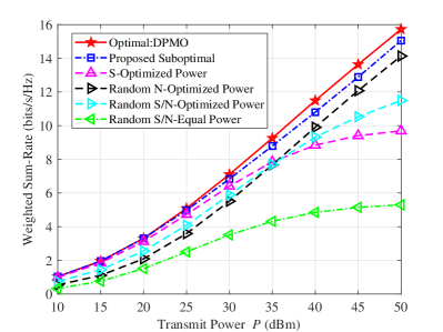
Figure 3: The weighted sum-rate of all users versus transmission power without considering QoS constraint: $Q=3$, $D=10$, $M=2$, $N=4$, $\delta_{M}=1$, $\delta_{N}=2$.

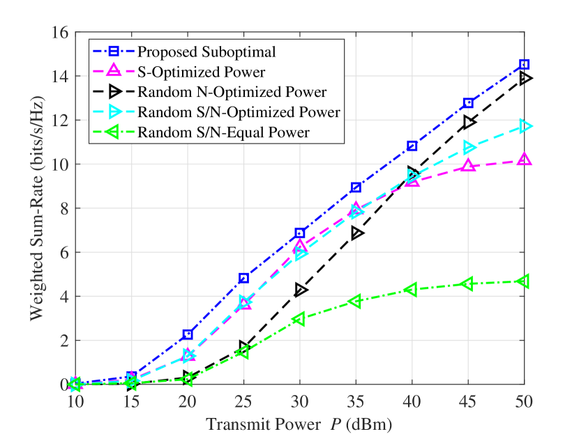
(a) Weighted Sum-Rate

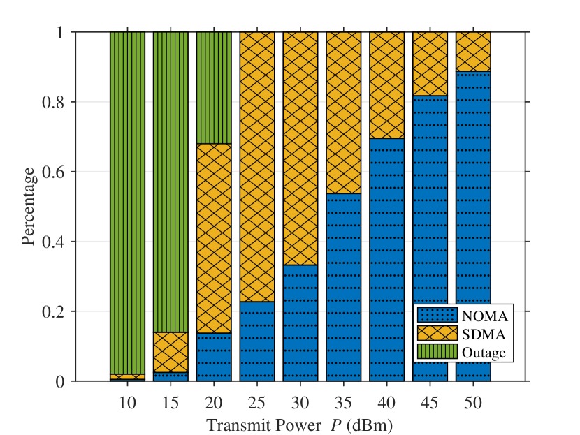
(b) Occurrence Percentage

Figure 4: The weighted sum-rate of all users versus transmission power with QoS constraint: $C_{\rm min}=0.6$, $Q=3$, $D=10$, $M=2$, $N=4$, $\delta_{M}=1$, $\delta_{N}=2$.

• S-Optimized Power: We implement SDMA for all DD RSs and then modify the SCA algorithm to solve the remaining power allocation problem.

• Random N-Optimized Power: We randomly select two users for each RS using the NOMA protocol, ensuring they satisfy constraint (67). Then, we modify the SCA algorithm to solve the power allocation problem.

• Random S/N-Optimized Power: We randomly choose between SDMA or NOMA for each DD RS, then select users for each RS while meeting constraint (67). Next, we modify the SCA algorithm to address the power allocation problem.

• Random S/N-Equal Power: We randomly choose between SDMA or NOMA for each DD RS, then select users for each RS while meeting constraint (67). Next, we apply equal power allocation to the users in each RS

Fig. 3 investigates the impact of transmission power on the weighted sum-rate without considering the individual rate constraint. Firstly, we observe that the weighted sum-rate of all schemes increases with the transmission power. But the performances in SDMA-based methods gradually saturate upon increasing the power. Because the MRT does not eliminate interference. Briefly, the powers of both the useful and the interference signals increase with the power, hence the SINR gradually approaches a constant value. By contrast, the NOMA-based baseline does not suffer from this phenomenon, because the utilization of SIC can eliminate the interference, and the SNR can increase with transmit power. Finally, the proposed sub-optimal algorithm can approach the performance of the optimal algorithm and outperform other baselines, which validates the effectiveness of the proposed algorithms.

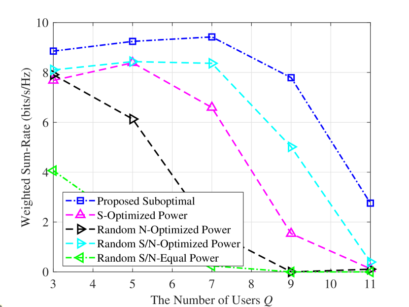
(a) Weighted Sum-Rate

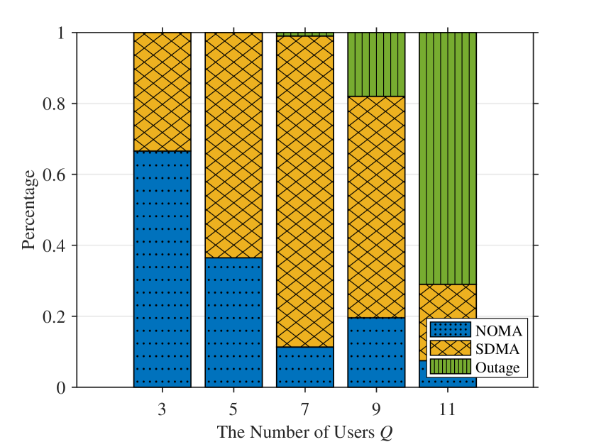
(b) Occurrence Percentage

Figure 5: The weighted sum-rate of all users versus the number of users with QoS constraint: $P=45$ dBm, $C_{\rm min}=0.6$, $D=8$, $M=3$, $N=8$, $\delta_{M}=1$, $\delta_{N}=2$.

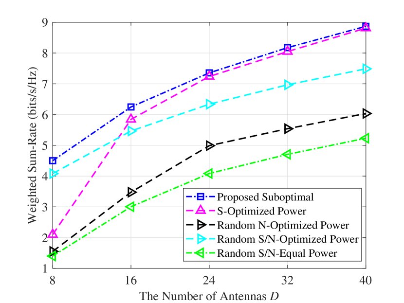
(a) Weighted Sum-Rate

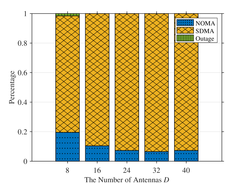
(b) Occurrence Percentage

Figure 6: The weighted sum-rate of all users versus the number of transmission antennas with QoS constraint: $P=45$ dBm, $C_{\rm min}=0.6$, $Q=3$, $M=18$, $N=16$, $\delta_{M}=6$, $\delta_{N}=8$.

Fig. 4 investigates the impact of transmission power on the weighted sum-rate of users, while considering the individual rate constraints. Firstly, we observe that the performances of all schemes degrade due to the rate constraints, especially when the transmission power is low. Then, the performance of the SDMA-based method is superior to that of the NOMA-based method at low transmission power because the latter struggles to effectively harness SIC. However, at a high transmission power, the performance of SDMA-based methods is limited by the interference, while the NOMA-based method benefits from the increase of power due to harnessing SIC. Hence, as the power increases, the proposed algorithm gradually shifts from favoring SDMA as the access scheme to favoring NOMA. Finally, the outage probability is reduced upon increasing the transmission power and the proposed algorithm outperforms the baselines.

Fig. 5 investigates the weighted sum-rate of users versus the number of users. Firstly, it shows that the performances of most schemes initially increase and then decrease as the number of users increases. The reason behind this trend is that the increased number of users can provide a higher degree of freedom for resource allocation, thus achieving an improved performance. However, the resources are limited and each newly added user has an individual minimal transmission rate. Hence, the outage probability will increase due to the increased additional contestants, which further decreases the performance. Furthermore, the performance of the SDMA-based method is relatively poorer compared to the NOMA-based method, when the number of users is low. However, as the number of users increases, the SDMA-based method exhibits superior performance compared to the NOMA-based method. This is attributed to the fact that for a smaller user count, the latter can apply SIC to cancel the interference, hence improving the transmission rate, while the latter readily meets the rate requirements without performing SIC for a sufficiently higher number of users. Therefore, as the number of users increases, the proposed algorithm gradually shifts from favoring SDMA to favoring NOMA. This validates the effectiveness of the proposed algorithms.

Fig. 6 investigates the weighted sum-rate of users versus the number of antennas. Firstly, it shows that the performances of all schemes increase with the number of antennas. The reason behind this trend is that the increased number of antennas can achieve higher beamforming gain, hence improving the SINR. Next, the performance of the SDMA-based method is relatively poorer compared to the NOMA-based method, when the number of antennas is low. However, as the number of antennas increases, the SDMA-based method exhibits superior performance compared to the NOMA-based method. Because upon increasing the number of antennas, the channels gradually become orthogonal. Thus, the SDMA-based method can simultaneously provide orthogonal transmissions to multiple users, whereas the NOMA-based method can only serve a maximum of two users. This leads to an increasing performance gap between them. Therefore, as the number of antennas increases, the proposed algorithm gradually shifts from favoring NOMA as the access scheme to favoring SDMA, which underlines the effectiveness of the advocated algorithm.

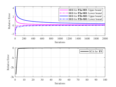
Figure 7: Convergence performances of BRB and SCA algorithms: $P=45$ dBm, $Q=3$, $D=10$, $M=2$, $N=4$, $\delta_{M}=1$, $\delta_{N}=2$.

Fig. 7 investigates the convergence performance of the BRB and SCA algorithms. Firstly, the upper and lower bounds of the BRB algorithm gradually approach each other and converge finally. Besides, the convergence speed of BRB in addressing SDMA-based problems is lower than that for NOMA-based problems. Because the former involves optimizing a higher number of variables. Finally, the SCA converges in just a few iterations, which confirms its low complexity.

VII Conclusions

We proposed an elastic multi-domain resource utilization mechanism for mobile communication and introduced a multi-user OTFS-MDMA system, which can leverage the associated user-specific channel characteristics across multi-domain resources including the DD, power, and spatial domains. Then, we formulated a weighted sum-rate maximization problem by jointly optimizing the user accommodation, access scheme selection, and power allocation subject to individual rate constraints and various other practical constraints. Since the problem formulated is a non-convex problem, we developed an efficient algorithm based on DPMO to find its globally optimal solution in the special case of disregarding rate constraints. Subsequently, we design a low-complexity SCA-SA algorithm to find its sub-optimal solutions in the general case. Finally, the simulation results demonstrate the benefits of employing elastic multi-domain resource utilization.

Note that the proposed sub-optimal algorithm still introduces some complexity that may affect the real-time application of OTFS-MDMA design, a potential solution is to more effectively approximate the original problem formulation and develop a lower-complexity sub-optimal algorithm. Besides, the proposed OTFS-MDMA design requires channel knowledge of all users. To reduce estimation overhead, we can incorporate channel temporal correlation and use learning-based methods [44] to allocate resources based on historical channel knowledge rather than current knowledge. However, as this paper focuses on the principle and validation of the OTFS-MDMA system design, we leave addressing the challenges of complexity and channel estimation overhead reduction in real-time applications as an interesting area for future work.

-A Derivation of (21)

In this part, we first introduce the following lemma in [14] and then apply it to prove the proposed theorem accordingly. Lemma 1 [14]: Let ${\bf{G}}={\rm{circ}}\left[{{{\bf{G}}_{0}},{{\bf{G}}_{1}},\cdots{{\bf{G}}_{N-1}}}\right]\in{\mathbb{C}}^{NM\times NM}$ be a block circulant matrix, where ${\bf G}_{n}\in{\mathbb{C}}^{M\times M}$ for $0\leq n\leq N-1$. Then, ${\bf{G}}$ can be re-expressed by a block diagonal matrix, i.e.,

$${\bf{G}} =\left({{\bf{F}}_{N}^{H}\otimes{{\bf{I}}_{M}}}\right){\rm{diag}}\left({{{\mbox{\boldmath{$\Theta$}}}_{i}},0\leq i\leq N-1}\right)\left({{{\bf{F}}_{N}}\otimes{{\bf{I}}_{M}}}\right)$$

$$= \left({{{\bf{F}}_{N}}\otimes{{\bf{I}}_{M}}}\right){\rm{diag}}\left({{{\tilde{\mbox{\boldmath{$\Theta$}}}}_{i}},0\leq i\leq N-1}\right)\left({{\bf{F}}_{N}^{H}\otimes{{\bf{I}}_{M}}}\right),$$

where ${{{\mbox{\boldmath{$\Theta$}}}_{i}}=\sum\limits_{n=0}^{N-1}{{{\bf{G}}_{n}}{e^{-{\rm{j2}}\pi\frac{{ni}}{{N}}}}}}$ and ${{\tilde{\mbox{\boldmath{$\Theta$}}}_{i}}=\sum\limits_{n=0}^{N-1}{{{\bf{G}}_{n}}{e^{{\rm{j2}}\pi\frac{{ni}}{{N}}}}}}$.

Based on this lemma, ${{\bf{H}}_{q}^{d}}$ can be represented by

$$\!\!\!\!{\bf{H}}_{q}^{d}=\left({{\bf{F}}_{N}^{H}\otimes{{\bf{I}}_{M}}}\right){\rm{diag}}\left({{\mbox{\boldmath{$\Theta$}}}_{q,0}^{d},\cdots,{\mbox{\boldmath{$\Theta$}}}_{q,N-1}^{d}}\right)\left({{{\bf{F}}_{N}}\otimes{{\bf{I}}_{M}}}\right),$$ (91)

where ${{\mbox{\boldmath{$\Theta$}}}_{q,i}^{d}=\sum\nolimits_{n=0}^{N-1}{{\bf{G}}_{q,n}^{d}{e^{-{\rm{j2}}\pi\frac{{ni}}{{N}}}},0\leq i\leq N-1}}$. Due to the definition of ${\bf{G}}_{q,n}^{d}$ in (20), we know ${\bf{G}}_{q,n}^{d}$ is a sum of $N$ circulant matrices, which means a similar diagonalization processes are present, i.e., ${\bf{G}}_{q,n}^{d}={{\bf{F}}_{M}}{\mbox{\boldmath{$\Lambda$}}}_{q,n}^{d}{\bf{F}}_{M}^{H}$ with ${\mbox{\boldmath{$\Lambda$}}}_{q,n}^{d}$ defined after (21). Then, we have

$${\bf{H}}_{q}^{d}=\left({{\bf{F}}_{N}^{H}\otimes{{\bf{F}}_{M}}}\right){\mbox{\boldmath{$\Lambda$}}}_{q}^{d}\left({{{\bf{F}}_{N}}\otimes{\bf{F}}_{M}^{H}}\right),$$ (92)

where ${\mbox{\boldmath{$\Lambda$}}}_{q}^{d}$ is defined after (21). Finally, we have (21).

References

• [1] H. Tataria, M. Shafi, A. F. Molisch, M. Dohler, H. Sjöland, and F. Tufvesson, “6G wireless systems: Vision, requirements, challenges, insights, and opportunities,” Proc. IEEE, vol. 109, no. 7, pp. 1166–1199, 2021.
• [2] Z. Zhang, Y. Xiao, Z. Ma, M. Xiao, Z. Ding, X. Lei, G. K. Karagiannidis, and P. Fan, “6G wireless networks: Vision, requirements, architecture, and key technologies,” IEEE Veh. Technol. Mag., vol. 14, no. 3, pp. 28–41, 2019.
• [3] X. Wang, J. Mei, S. Cui, C.-X. Wang, and X. S. Shen, “Realizing 6G: The operational goals, enabling technologies of future networks, and value-oriented intelligent multi-dimensional multiple access,” IEEE Netw., vol. 37, no. 1, pp. 10–17, 2023.
• [4] C. Xu, X. Zhang, P. Petropoulos, S. Sugiura, R. G. Maunder, L.-L. Yang, Z. Wang, J. Yuan, H. Haas, and L. Hanzo, “Optical OTFS is capable of improving the bandwidth-, power-and energy-efficiency of optical OFDM,” IEEE Trans. Commun., vol. 72, no. 2, pp. 938–953, 2024.
• [5] S. K. Mohammed, R. Hadani, A. Chockalingam, and R. Calderbank, “OTFS—A mathematical foundation for communication and radar sensing in the delay-doppler domain,” IEEE BITS Inf. Theory Mag., vol. 2, no. 2, pp. 36–55, 2022.
• [6] R. Hadani, S. Rakib, M. Tsatsanis, A. Monk, A. J. Goldsmith, A. F. Molisch, and R. Calderbank, “Orthogonal time frequency space modulation,” in Proc. IEEE Wireless Commun. Netw. Conf. (WCNC), 2017, pp. 1–6.
• [7] B. S. Reddy, C. Velampalli, and S. S. Das, “Performance analysis of multi-user OTFS, OTSM, and single carrier in uplink,” IEEE Trans. Commun., 2023.
• [8] Z. Wei, W. Yuan, S. Li, J. Yuan, G. Bharatula, R. Hadani, and L. Hanzo, “Orthogonal time-frequency space modulation: A promising next-generation waveform,” IEEE Wireless Commun., vol. 28, no. 4, pp. 136–144, 2021.
• [9] Z. Sui, H. Zhang, S. Sun, L.-L. Yang, and L. Hanzo, “Space-time shift keying aided OTFS modulation for orthogonal multiple access,” IEEE Trans. Commun., vol. 71, no. 12, pp. 7393–7408, 2023.
• [10] H. Lin and J. Yuan, “Orthogonal delay-doppler division multiplexing modulation,” IEEE Trans. Wireless Commun., vol. 21, no. 12, pp. 11 024–11 037, 2022.
• [11] L. Gaudio, G. Colavolpe, and G. Caire, “OTFS vs. OFDM in the presence of sparsity: A fair comparison,” IEEE Trans. Wireless Commun., vol. 21, no. 6, pp. 4410–4423, 2021.
• [12] M. Mohammadi, H. Q. Ngo, and M. Matthaiou, “Cell-free massive MIMO with OTFS modulation: Statistical CSI-based detection,” IEEE Wireless Commun. Lett., vol. 12, no. 6, pp. 987–991, 2023.
• [13] S. Li, J. Yuan, P. Fitzpatrick, T. Sakurai, and G. Caire, “Delay-doppler domain tomlinson-harashima precoding for OTFS-based downlink MU-MIMO transmissions: Linear complexity implementation and scaling law analysis,” IEEE Trans. Commun., vol. 71, no. 4, pp. 2153–2169, 2023.
• [14] P. Raviteja, Y. Hong, E. Viterbo, and E. Biglieri, “Practical pulse-shaping waveforms for reduced-cyclic-prefix OTFS,” IEEE Trans. Veh. Technol., vol. 68, no. 1, pp. 957–961, 2018.
• [15] S. Tiwari, S. S. Das, and V. Rangamgari, “Low complexity lmmse receiver for otfs,” IEEE Commun. Lett., vol. 23, no. 12, pp. 2205–2209, 2019.
• [16] P. Raviteja, K. T. Phan, Y. Hong, and E. Viterbo, “Interference cancellation and iterative detection for orthogonal time frequency space modulation,” IEEE Trans. Wireless Commun., vol. 17, no. 10, pp. 6501–6515, 2018.
• [17] Z. Yuan, F. Liu, W. Yuan, Q. Guo, Z. Wang, and J. Yuan, “Iterative detection for orthogonal time frequency space modulation with unitary approximate message passing,” IEEE Trans. Wireless Commun., vol. 21, no. 2, pp. 714–725, 2021.
• [18] Z. Wei, W. Yuan, S. Li, J. Yuan, and D. W. K. Ng, “Off-grid channel estimation with sparse Bayesian learning for OTFS systems,” IEEE Trans. Wireless Commun., vol. 21, no. 9, pp. 7407–7426, 2022.
• [19] A. Mehrotra, S. Srivastava, S. Asifa, A. K. Jagannatham, and L. Hanzo, “Online bayesian learning aided sparse CSI estimation in OTFS modulated MIMO systems for ultra-high-doppler scenarios,” IEEE Trans. Commun., vol. 72, no. 4, pp. 2182–2200, 2024.
• [20] V. Khammammetti and S. K. Mohammed, “Spectral efficiency of OTFS based orthogonal multiple access with rectangular pulses,” IEEE Trans. Veh. Technol., vol. 71, no. 12, pp. 12 989–13 006, 2022.
• [21] S. Habibi, J. Chen, F. Fang, and X. Wang, “User-specific channel estimation overhead optimization and resource allocation for multi-user OTFS systems,” IEEE Commun. Lett., 2024.
• [22] Z. Ding, R. Schober, P. Fan, and H. V. Poor, “OTFS-NOMA: An efficient approach for exploiting heterogenous user mobility profiles,” IEEE Trans. Commun., vol. 67, no. 11, pp. 7950–7965, 2019.
• [23] Y. Ge, Q. Deng, P. Ching, and Z. Ding, “OTFS signaling for uplink NOMA of heterogeneous mobility users,” IEEE Trans. Commun., vol. 69, no. 5, pp. 3147–3161, 2021.
• [24] Y. Ge, Q. Deng, D. González, Y. L. Guan, and Z. Ding, “OTFS signaling for SCMA with coordinated multi-point vehicle communications,” IEEE Trans. Veh. Technol., vol. 72, no. 7, pp. 9044–9057, 2023.
• [25] Y. Ma, G. Ma, N. Wang, Z. Zhong, and B. Ai, “OTFS-TSMA for massive internet of things in high-speed railway,” IEEE Trans. Wireless Commun., vol. 21, no. 1, pp. 519–531, 2021.
• [26] M. Li, S. Zhang, F. Gao, P. Fan, and O. A. Dobre, “A new path division multiple access for the massive MIMO-OTFS networks,” IEEE J. Sel. Areas Commun., vol. 39, no. 4, pp. 903–918, 2020.
• [27] C. Liu, S. Li, W. Yuan, X. Liu, and D. W. K. Ng, “Predictive precoder design for OTFS-enabled URLLC: A deep learning approach,” IEEE J. Sel. Areas Commun., vol. 41, no. 7, pp. 2245–2260, 2023.
• [28] Y. Liu, X. Wang, G. Boudreau, A. B. Sediq, and H. Abou-Zeid, “A multi-dimensional intelligent multiple access technique for 5G beyond and 6G wireless networks,” IEEE Trans. Wireless Commun., vol. 20, no. 2, pp. 1308–1320, 2020.
• [29] Y. Liu, X. Wang, J. Mei, G. Boudreau, H. Abou-Zeid, and A. B. Sediq, “Situation-aware resource allocation for multi-dimensional intelligent multiple access: A proactive deep learning framework,” IEEE J. Sel. Areas Commun., vol. 39, no. 1, pp. 116–130, 2020.
• [30] J. Mei, W. Han, X. Wang, and H. V. Poor, “Multi-dimensional multiple access with resource utilization cost awareness for individualized service provisioning in 6G,” IEEE J. Sel. Areas Commun., vol. 40, no. 4, pp. 1237–1252, 2022.
• [31] Y. Sun, D. W. K. Ng, Z. Ding, and R. Schober, “Optimal joint power and subcarrier allocation for full-duplex multicarrier non-orthogonal multiple access systems,” IEEE Trans. Commun., vol. 65, no. 3, pp. 1077–1091, 2017.
• [32] J. Chen, L. Zhang, Y.-C. Liang, and S. Ma, “Optimal resource allocation for multicarrier NOMA in short packet communications,” IEEE Trans. Veh. Technol., vol. 69, no. 2, pp. 2141–2156, 2019.
• [33] Z. Wei, W. Yuan, S. Li, J. Yuan, and D. W. K. Ng, “Transmitter and receiver window designs for orthogonal time-frequency space modulation,” IEEE Trans. Commun., vol. 69, no. 4, pp. 2207–2223, 2021.
• [34] P. Raviteja, E. Viterbo, and Y. Hong, “OTFS performance on static multipath channels,” IEEE Wireless Commun. Lett., vol. 8, no. 3, pp. 745–748, 2019.
• [35] F. Liu, Z. Yuan, Q. Guo, Z. Wang, and P. Sun, “Message passing-based structured sparse signal recovery for estimation of OTFS channels with fractional doppler shifts,” IEEE Trans. Wireless Commun., vol. 20, no. 12, pp. 7773–7785, 2021.
• [36] S. Li, W. Yuan, Z. Wei, and J. Yuan, “Cross domain iterative detection for orthogonal time frequency space modulation,” IEEE Trans. Wireless Commun., vol. 21, no. 4, pp. 2227–2242, 2021.
• [37] Y. Zhang, X. Zhu, Y. Liu, Y. Jiang, Y. L. Guan, D. González, and V. K. Lau, “A cross-domain iterative OTFS receiver for sparse doubly selective channels,” IEEE Wireless Commun. Lett., vol. 13, no. 1, pp. 54–58, 2024.
• [38] W. U. Khan, F. Jameel, T. Ristaniemi, S. Khan, G. A. S. Sidhu, and J. Liu, “Joint spectral and energy efficiency optimization for downlink NOMA networks,” IEEE Trans. Cogn. Commun. Netw., vol. 6, no. 2, pp. 645–656, 2019.
• [39] J. Chen, X. Wang, and Y.-C. Liang, “Impact of channel aging on dual-function radar-communication systems: Performance analysis and resource allocation,” IEEE Trans. Commun., vol. 71, no. 8, pp. 4972–4987, 2023.
• [40] J. Zhu, J. Wang, Y. Huang, S. He, X. You, and L. Yang, “On optimal power allocation for downlink non-orthogonal multiple access systems,” IEEE J. Sel. Areas Commun., vol. 35, no. 12, pp. 2744–2757, 2017.
• [41] H. Chen, D. Zhao, Q. Chen, and R. Chai, “Joint computation offloading and radio resource allocations in small-cell wireless cellular networks,” IEEE Trans. Green Commun. Netw., vol. 4, no. 3, pp. 745–758, 2020.
• [42] H. Chen, T. D. Todd, D. Zhao, and G. Karakostas, “Wireless and service allocation for mobile computation offloading with task deadlines,” IEEE Trans. Mob. Comput., vol. 23, no. 5, pp. 5054–5068, 2024.
• [43] P. Jia and X. Wang, “A new virtual network topology based digital twin for spatial-temporal load-balanced user association in 6G HetNets,” IEEE J. Sel. Areas Commun., vol. 41, no. 10, pp. 3080–3094, 2023.
• [44] J. Chen and X. Wang, “Learning-based intermittent CSI estimation with adaptive intervals in integrated sensing and communication systems,” arXiv preprint arXiv:2405.14724, 2024.
• [45] Y. J. A. Zhang, L. Qian, and J. Huang, “Monotonic optimization in communication and networking systems,” Found. Trends Netw., vol. 7, no. 1, pp. 1–75, 2013.
• [46] E. Björnson, G. Zheng, M. Bengtsson, and B. Ottersten, “Robust monotonic optimization framework for multicell MISO systems,” IEEE Trans. Signal Process., vol. 60, no. 5, pp. 2508–2523, 2012.
• [47] M. Grant, S. Boyd, and Y. Ye, “CVX: MATLAB software for disciplined convex programming,” [Online]. Available: http://stanford.edu/ boyd/cvx.
• [48] B. Di, L. Song, and Y. Li, “Sub-channel assignment, power allocation, and user scheduling for non-orthogonal multiple access networks,” IEEE Trans. Wireless Commun., vol. 15, no. 11, pp. 7686–7698, 2016.
• [49] L. Shan, S. Gao, Y. Yu, F. Zhang, Y. Hu, Y. Wang, and M. Chen, “Resource allocation for multi-cell multi-timeslot transmission: Centralized and distributed algorithms,” IEEE Trans. Netw. Service Manag., vol. 21, no. 3, pp. 3021–3034, 2024.
• [50] J. Chen, L. Zhang, Y.-C. Liang, X. Kang, and R. Zhang, “Resource allocation for wireless-powered IoT networks with short packet communication,” IEEE Trans. Wireless Commun., vol. 18, no. 2, pp. 1447–1461, 2019.
• [51] A. Nemirovskii, “Interior point polynomial algorithms in convex programming,” 2004, [Online]. Available: https://www2.isye.gatech.edu/~nemirovs/Lect_IPM.pdf.
• [52] M. Mohammadi, H. Q. Ngo, and M. Matthaiou, “Cell-free massive MIMO meets OTFS modulation,” IEEE Trans. Commun., vol. 70, no. 11, pp. 7728–7747, 2022.