Application of Physics-Informed Neural Networks in Removing Telescope Beam Effects

Abstract

This study introduces $\tt{PI-AstroDeconv}$, a physics-informed semi-supervised learning method specifically designed for removing beam effects in astronomical telescope observation systems. The method utilizes an encoder-decoder network architecture and combines the telescope’s point spread function or beam as prior information, while integrating fast Fourier transform accelerated convolution techniques into the deep learning network. This enables effective removal of beam effects from astronomical observation images. $\tt{PI-AstroDeconv}$ can handle multiple PSFs or beams, tolerate imprecise measurements to some extent, and significantly improve the efficiency and accuracy of image deconvolution. Therefore, this algorithm is particularly suitable for astronomical data processing that does not rely on annotated data. To validate the reliability of the algorithm, we used the SKA Science Data Challenge 3a datasets and compared it with the $\tt{CLEAN}$ deconvolution method at the 2-D matter power spectrum level. The results demonstrate that our algorithm not only restores details and reduces blurriness in celestial images at the pixel level but also more accurately recovers the true neutral hydrogen power spectrum at the matter power spectrum level.

1 Introduction

In the universe, there are various types of astronomical signals originating from the electromagnetic radiation emitted by celestial bodies, systems, or cosmic phenomena (Rohlfs & Wilson, 2013; Gudel, 2002). These signals reveal the nature and characteristics of the cosmic space and are crucial sources of information for humanity’s exploration of the universe. Examples of such signals are numerous, including cosmic microwave background radiation, radiation from galaxies and galaxy clusters, and starlight (de Bernardis et al., 2000; Martin & Irvine, 1983; Davis et al., 1985; Springel et al., 2006). Observing these different types of astronomical signals often requires specially designed telescopes, such as radio telescopes, infrared telescopes, optical telescopes, and X-ray telescopes. The beam width of a telescope is proportional to the wavelength it observes; that is, the longer the wavelength, the wider the beam. However, a beam that is too wide can affect the image clarity and detail resolution. Therefore, different telescope designs and technologies are needed to optimize observational results. Although radio telescopes have a relatively wide beam, their longer wavelengths provide stronger penetration capabilities, allowing them to observe interstellar dust and gas through the Earth’s atmosphere. Similarly, due to their longer wavelengths, radio telescopes can expand the observational area through large antenna arrays and improve spatial resolution. Consequently, radio telescopes play a crucial role in detecting and collecting radio waves from celestial radiation, making them ideal tools for exploring distant and mysterious cosmic phenomena such as black holes and dark matter (Schwab, 1984; Burns et al., 2012).

In recent years, the field of astronomy has achieved numerous breakthroughs and advancements, largely due to the rapid development of astronomical telescopes and related technologies. Among these, radio astronomy has seen significant success, with major radio telescopes such as FAST (Nan et al., 2011; Li et al., 2012, 2018), the Arecibo Observatory (Drake & Sagan, 1973; The Staff at the National Astronomy and Ionosphere Center, 1975; Mathews, 2013), the Very Large Array (Napier et al., 1983; Perley et al., 2011; Kellermann et al., 2020), MeerKAT (Camilo et al., 2018; Sorgho et al., 2018), CHIME (Bandura et al., 2014; Collaboration et al., 2018), LOFAR (Vermeulen & van Haarlem, 2011; Röttgering, 2003; de Vos et al., 2009), ASKAP (Johnston et al., 2007; Johnston & Wall, 2008), and MWA (Tingay et al., 2013; Lonsdale et al., 2009) playing crucial roles in advancing our understanding of the universe. The progress in radio astronomy is closely related to the capabilities of aperture synthesis arrays, which form images by cross-correlating signals from a series of antennas. Traditional imaging assumes a uniform primary beam pattern at all locations. MeerKAT, ASKAP, and MWA are precursor projects to the Square Kilometre Array (SKA) (Santos et al., 2015; Bull et al., 2015; Bacon et al., 2020), an international radio telescope construction initiative. Many telescopes are expected to be incorporated into the SKA project. With its high sensitivity and resolution, the SKA is set to provide unparalleled observational data.

However, as the world’s largest future synthetic aperture radio telescope system, the SKA faces significant challenges in imaging, including vast amounts of data, complex data management requirements, and the diversity of primary beam patterns (WU et al., 2015; Wang et al., 2020b; Spinelli et al., 2021). The size of the antenna beam, which is the sensitive area for receiving radio waves, affects the imaging quality between antennas, especially in continuous wave interferometry for celestial imaging. The resolution of celestial imaging is determined jointly by the distance between antennas and the size of the beam. Given the large number of antennas in the SKA, such as ASKAP in the central-western region of Australia, which consists of 36 dish antennas with baselines up to 6 kilometers, and MeerKAT in the Northern Cape Province of South Africa, which consists of 64 antennas with baselines up to 8 kilometers, the beam size of these telescopes significantly impacts imaging quality (Alexander et al., 2011; Williamson et al., 2021; Mort et al., 2016; Dodson et al., 2022). Interferometer baselines can be significantly larger compared to single-dish telescopes, and smaller beams can provide higher spatial and observational resolution, allowing them to detect weaker astronomical signals. However, smaller beams, due to their limited radio wave coverage, lead to a decrease in signal strength, which affects data quality. To achieve sufficient signal-to-noise ratio, data collected through the SKA will require longer integration times or more advanced data processing techniques, ultimately affecting imaging quality. Therefore, researchers must carefully consider the impact of antenna beam patterns in the SKA when conducting research and developing observations.

In the field of data processing for radio telescopes, the $\tt{CLEAN}$ deconvolution algorithm plays a crucial role. Since its introduction by Högbom in 1974 (Hogbom, 1974), it has not only revolutionized the technology of radio synthesis imaging but also significantly accelerated the development of the entire fielde (Cornwell, 2009; Rich et al., 2008). The efficiency of the $\tt{CLEAN}$ algorithm stems from its ability to identify and mitigate the effects of point source components in the point spread function (PSF), thereby accurately reconstructing the brightness distribution of the sky (Cornwell, 1983). The algorithm is particularly effective for celestial objects that can be approximated with a small number of parameters, which typically appear as a few widely distributed point sources in the imaging field. However, the $\tt{CLEAN}$ algorithm also has some notable drawbacks. For example, its deconvolution performance is less effective for extended sources with continuous intensity distributions. Additionally, when processing large amounts of interferometer data, the $\tt{CLEAN}$ algorithm requires substantial computational resources and has relatively slow processing speeds. Moreover, the algorithm relies on researchers having a solid background in astronomical data processing to set the parameters appropriately. Improper parameter settings can lead to underfitting or overfitting issues. With the continuous advancement of radio telescope technology, there is an increasing demand for more complex deconvolution algorithms. To meet this demand, various derivative versions of the $\tt{CLEAN}$ algorithm have emerged, such as $\tt{Clark}$ (Clark, 1980), $\tt{Cotton-Schwab}$ (Schwab & Cotton, 1983; Schwab, 1984), $\tt{MS-CLEAN}$ (Wakker & Schwarz, 1988; Cornwell, 2008), and $\tt{WSClean}$ (Offringa et al., 2014; Offringa & Smirnov, 2017; Van der Tol et al., 2018). These derivative algorithms retain the advantages of the $\tt{CLEAN}$ algorithm while further enhancing the capability to process complex astronomical data.

In recent years, with the gradual advancement of artificial intelligence technology, deep learning algorithms have been applied to address issues such as beam effects in radio telescopes (An et al., 2019; Ni et al., 2022; Schmidt et al., 2022; Chiche et al., 2023). Generally, deep learning algorithms have a strong dependence on the quantity and quality of training data and labeled data, which is particularly crucial in the field of astronomy where data labeling is essential. Historically, the application of deep learning algorithms in astronomy has been limited due to the difficulty in obtaining high-quality data. To address this issue and facilitate image deconvolution and reconstruction, we have introduced an unsupervised network architecture that integrates physical prior information, named $\tt{PI-DeconvAstro}$ (Ni et al., 2024). This network employs an encoder-decoder structure and utilizes the telescope’s point spread function (PSF) or beam as prior knowledge. We tested the network using the SKA Science Data Challenge 3a (SDC3a)  datasets and compared the algorithm with the $\tt{CLEAN}$ deconvolution algorithm at the level of the matter power spectra.

The structure of the remainder of this paper is organized as follows: Section 1 provides an introduction, Section 2 discusses data simulation and preprocessing, Section 3 elaborates on the deconvolution process, Section 4 presents the results and discussion, and Section 5 concludes the paper.

2 Data Simulation and Pre-Processing

In radio astronomy, interferometric array technology is a crucial observational method that significantly enhances the sensitivity and resolution for detecting radiation signals from celestial bodies through the coordinated observations of multiple antenna elements. However, in actual observations, data are often affected by various factors, such as the telescope’s beam effects and interference from the Milky Way and extragalactic sources, which can introduce errors and noise into the observational results (Makinen et al., 2021; Ni et al., 2022; Gao et al., 2023). To extract valuable astronomical information from raw observational data, meticulous data simulation and preprocessing are required. This chapter delves into this process, providing a detailed description of the data simulation specifics for SDC3a and conducting simulations based on the relevant parameters of SDC3a.

2.1 Telescope Model and Foreground Model

The principle of aperture synthesis technology involves combining signals from multiple telescopes using interferometric techniques to achieve high-resolution image reconstruction (Högbom, 1974). The key is to arrange the telescopes in an array and observe the same light source simultaneously (Wilson et al., 2009; Thompson et al., 2017a). Each telescope receives signals that carry phase information, reflecting the spatial structure of the source. In aperture synthesis, the first step is to process these signals for correlation, which is typically achieved through Fourier transformation. Fourier transformation converts signals from the time domain to the frequency domain, allowing for the measurement and recording of phase differences. By measuring the amplitude and phase of the correlated signals and performing appropriate data processing and analysis, high-resolution images can be reconstructed(Thompson et al., 2017b).

The SDC3a simulation project represents the third Science Data Challenge of the SKA radio telescope, with its core objective being the effective separation of foreground contamination signals from the Milky Way and extra-galactic sources to reveal the pristine neutral hydrogen (HI) signal. In the SDC3a simulation, the $\tt{OSKAR}$  software package is employed to generate visibilities, which are produced based on specific time and frequency sampling (Hamaker, 2006; Mort et al., 2010; Dewdney et al., 2017). The telescope model is based on the SKA-Low configuration, simulating the “Vogel” layout that includes 512 stations, a single-arm spiral configuration designed to achieve uniform antenna area density and maximized azimuthal angle sampling. To reduce computational costs, a single station layout was adopted in the simulation rather than $512$ distinct station layouts. This simplification resulted in an increased response in the far side-lobes, for which compensation was made in the definition of the foreground model.

The foreground model consists of two parts: the “outer” component covering a $2\pi$ steradian volume above the horizon and the “inner” component defining a more limited field of view near the pointing direction. The external component includes the A-Team sources with brightness exceeding several hundred Jy and sources from the $\tt{GLEAM}$ catalogue for which a composite $\tt{GLEAM}$ and $\tt{LoBES}$ $\tt{OSKAR}$ model file was kindly made available for use in these simulations (Wayth et al., 2015; Lynch et al., 2021). All sources with a brightness exceeding $5~{}\mathrm{Jy}$ at $150~{}\mathrm{MHz}$ (approximately $1200$ sources) are included in the external sky model. These sources, located in the far side-lobe regions of the observation, are typically modeled and removed through a “deconvolution” process during the observation and imaging procedures. To simulate the attenuation of these sources, a net attenuation factor of $10^{-3}$ is assumed.

The inner foregound model is an integral component of radio astronomical simulations, accurately depicting the distribution of sky sources at the observational frequency. This model is anchored on the first null of the station beam pattern at the minimum observational frequency, ensuring high-fidelity in the simulation. The model encompasses all sources from the $\tt{GLEAM}$ and $\tt{LoBES}$ catalogues with a $150~{}\mathrm{MHz}$ flux density exceeding $100~{}\mathrm{mJy}$, spatially represented through Gaussian models. For sources with a flux density below $100$ , the model employs the $\tt{T-RECS}$  code for simulation, extending down to a flux density of $1\mathrm{mJy}$, over an $8\times 8~{}\mathrm{degree}$ simulation area (Lucherini et al., 2021). The model utilizes a $5\times 5~{}\mathrm{arcsec}$ pixel sampling with a $10\times 10$ $\mathrm{arcsec}$ FWHM Gaussian gridding kernel to normalize the data to units of $\mathrm{Jy/pixel}$, facilitating analysis and comparison. Within the model, pixels brighter than $10^{-5}~{}\mathrm{Jy/pixel}$ are considered as Gaussian source model components with a $10\times 10~{}\mathrm{arcsec}$ extent, having a flux density equivalent to the pixel’s brightness, and a spectral index set to zero. The model is also updated for each observational frequency to track the spectral energy density variations of $\tt{T-RECS}$ sources, adapting to the characteristics of sources under different observational conditions. This detailed inner sky simulation provides a robust foundation for radio astronomical data processing, especially in dealing with beam effects and foreground interference.

The inner foreground model’s additional components were created using a coarser 512x512 pixel grid with $56.25\times 56.25$ arcsec sampling, balancing accuracy with computational demands. This resolution matches the $\tt{GSM2016}$ (Zheng et al., 2017) sky model’s evaluation at various observing frequencies. To address $\tt{GSM2016}$’s limited angular resolution at low radio frequencies, the model was enhanced with $\tt{MHD}$ simulation data (Sault et al., 1995; Jelic et al., 2008), capturing filamentary structures down to the $\mathrm{arcmin}$ scale and scaled to $\mathrm{Jy/pixel}$. Furthermore, faint extra-galactic sources from the residual $\tt{T-RECS}$ image were smoothed and resampled to fit the “inner” foreground model grid, using appropriate normalization for the coarser sampling. This approach ensures a comprehensive representation of the sky for radio astronomical simulations.

2.2 EoR Signal and Error Model

The signal data from the Epoch of Reionization (EoR) is derived from $\tt{21cmFAST}$  simulations. This simulation technique can generate three-dimensional cosmic evolution scenarios, including detailed representations of density, ionization fraction, peculiar velocity, and spin temperature fields. These integrated fields are further used to derive the brightness temperature distribution at a 21 cm wavelength (Mesinger et al., 2011; Park et al., 2019; Murray et al., 2020; Muñoz et al., 2022). The $\tt{21cmFAST}$ ensures swift prediction of the 21-cm signal while maintaining simulation speed and efficiency, enabling efficient computation on a single processor (Mesinger et al., 2011).

In the process of the 21-cm simulation, a set of fixed cosmological parameters were selected, which are based on the best-fit values obtained from the $\it{Planck}$ 2018 data (Aghanim et al., 2020). The CMB temperature is $T_{\text{CMB}}=2.7255\,\text{K}$. The matter density is $\Omega_{\text{m}}=0.30964$, while the dark energy density is $\Omega_{\Lambda}=0.69036$. The Hubble constant is given by $H_{0}=100\,\text{km}\,\text{s}^{-1}\,\text{Mpc}^{-1}$. The effective number of neutrino species is $N_{\text{eff}}=3.046$, with three neutrino masses specified as $m_{\text{nu}}=[0,0,0.06]\,\text{eV}$. The baryon density is $\Omega_{\text{b}}=0.04897$.

To enhance the realism of the simulation, SDC3a incorporated various instrumental noises into the simulation process. They artificially attenuated the brightness of sources in the ”outer” sky model beyond the central 8x8 degrees with a factor of $10^{-3}$, simulating a partially successful all-sky source population modeling and subtraction. This attenuation reflects the differences in far side-lobe responses due to diverse station layouts and the precision of source modeling and subtraction (Dewdney et al., 2017).

2.3 Simulated Images

During the simulation process, the $\tt{OSKAR}$ software utilizes specific telescope, sky, and error models to generate visibility data. Images are then created from this visibility data, forming “natural” weighted images that have not undergone deconvolution, along with their corresponding synthesized beams (Offringa et al., 2014; Bean et al., 2022). Once the images and PSF for all frequency channels are ready, they are assembled into a data cube for subsequent analysis.

During the simulation process, the signal, foreground, and noise components were represented as $N\times 512\times 512$ pixel cubes, where $N$ denotes the number of frequency channels. However, when extracting the visibility function, we skillfully employed the oversampling parameter to optimize the output to an $N\times 2048\times 2048$ pixels cube. This strategy significantly improved the precision of data processing, resulting in more accurate images (Hjellming, 1989).

If only a small region of the sky needs to be mapped, the visibility $V(u,v,w)$ can be represented as follows (Thompson et al., 2017b):

$$V(u,v,w)=\int_{-\infty}^{+\infty}\int_{-\infty}^{+\infty}A(x,y)I(x,y)e^{i2\pi(ux+vy+w)}dxdy,$$ (1)

where $A(x,y)$ is the effective area of a plane perpendicular to the x and y directions, and $I(x,y)$ is intensity distribution.

Convert the observed phase of $V(u,v,w)$ to the $uv$-plane, $V(u,v,w)\simeq V(u,v,0)e^{i2\pi w}$. Then, perform the inverse Fourier transform on equation (1), and we can obtain

$$I^{\prime}(x,y)=A(x,y)I(x,y)=\int_{-\infty}^{+\infty}V(u,v,0)e^{-i2\pi(ux+vy)}dudv,$$ (2)

where $I^{\prime}(x,y)$ is the intensity $I(x,y)$ as modified by the primary beam shape $A(x,y)$. One can easily correct $I^{\prime}(x,y)$ by dividing it, pixel by pixel, by $A(x,y)$. By solving equation (2), the aperture synthesis can be derived from the varying I(x, y) values among different sources. However, this necessitates a substantial computational capacity. To simplify the problem, we have to grid the visibility function and weight it by a grading function, $g(u,v)$. We can obtain an image via a discrete Fourier transform(DFT):

$$I_{D}(x,y)=\sum_{k}g(u_{k},v_{k})V(u_{k},v_{k})e^{-i2\pi(u_{k}x+v_{k}y)}.$$ (3)

Comparing Equation (2) and Equation (3), we can derive the following relationship

$$I_{D}(x,y)=P_{D}(x,y)\otimes I^{\prime}(x,y),$$ (4)

where $\otimes$ means convolution, and

$$P_{D}=\sum_{k}g(u_{k},v_{k})e^{-i2\pi(u_{k}x+v_{k}y)}.$$ (5)

The $P_{D}$ is response to a point source, which is PSF. It is worth noting that in the subsequent construction of the deep learning network, we will innovatively introduce $P_{D}$ as prior physical information and deeply integrate it into the network architecture. This strategy aims to leverage the guiding role of physical knowledge to achieve deconvolution while ensuring the interpretability and accuracy of the results.

Since we are not concerned with the weighting method but rather with examining the effects of deconvolution, we use “natural” weighting throughout this work. This approach avoids assigning weights to samples before gridding, ensuring that regions with more baselines do not dominate the final image formation. This method avoided assigning weights to samples prior to gridding, ensuring that regions with more baselines did not dominate the formation of the final image.

The specific characteristics of the data have been meticulously documented in Table 1, which includes parameters such as the observation track length ($\text{HA}$), thermal noise equivalent (${\text{N}}_{\text{thermal}}$), field of view ($\text{FoV}$), integration time ($\text{Ti}$), channel width ($\Delta\text{f}$), frequency coverage (${\text{f}}_{\text{cov}}$), Pixel size ($\text{px}$), and Number of pixels (${\text{N}}_{\text{pix}}$).

Additionally, the SDC3a simulation incorporates various ancillary data, including synthesized beam and time-varying station beams at each frequency, station and antenna layouts, and thermal noise models. These detailed parameter settings facilitate subsequent analysis and discussion. Table 1 not only encapsulates the key parameters of the dataset but also provides essential insights for further exploration of the data’s properties. Through a rigorous examination of these data features, our aim is to attain a more profound comprehension of the simulation outcomes and to offer robust foundational support for future research endeavors.

Parameters	HI	$N_{thermal}$	FoV(RA, Dec)	Ti	$f_{conv}$	$\Delta f$	$N_{pix}$	pix
[UNIT]	[Hours]	[Hours]	[deg]	[sec]	[MHz]	[KHz]	[No.]	[arcsec]
Values	$[-2,2]$	$1000$	$[-30,0]$	$10$	$106-196$	$100$	$512\times 512$	$16\times 16$

Table 1: General parameters, measurement set configurations, and image cube specifications for the $\tt{21cmFAST}$ simulation.

To thoroughly investigate the spatial characteristics of the SDC3a simulation data, we have constructed a 3D image, as shown in Figure 1. Within this figure, the $xy$-plane corresponds to the scale distribution in the celestial coordinate system. Specifically, the $x$-axis represents the declination coordinate, the $y$-axis denotes the right ascension coordinate, and the $z$-axis symbolizes the line-of-sight direction, or the frequency axis direction. Given that the core region of the SDC3a simulation is concentrated on the central area of the $xy$-plane, namely the central $512\times 512$ pixels of that plane, we have deliberately selected and displayed only the details of this central region in the presented image. The bright regions in the figure represent the distribution of galaxy clusters.

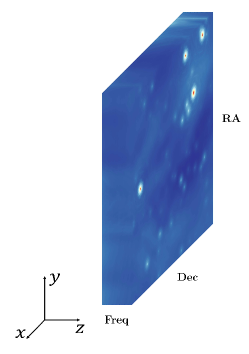
Figure 1: SDC3a simulation image schematic. The $xy$-plane represents scale, with the $x$-axis indicating Declination and the $y$-axis representing Right Ascension. The $z$-axis denotes the line of sight direction, which corresponds to the frequency direction. The bright regions represent the distribution of galaxy clusters.

3 De-convolution

In the data processing of radio astronomy, deconvolution techniques play a critical role by minimizing the limitations of visibility measurements. The visibility function has two main shortcomings that constrain the accuracy of aperture synthesis imaging: limited spatial frequency coverage and inherent errors in the visibility function. Deconvolution techniques can effectively address these deficiencies.

Based on the $\tt{CLEAN}$ algorithm, various deconvolution algorithms have been developed and they perform excellently in astronomical image deconvolution. Deep learning algorithms like $\tt{PI-AstroDeconv}$ offer new approaches to deconvolution. This chapter will primarily focus on the performance and application of $\tt{WSClean}$, as well as the $\tt{PI-AstroDeconv}$ algorithm.

3.1 WSClean Algorithm

In the data processing of radio astronomy, due to the incomplete coverage of the $\tt{uv}$ plane, the resulting dirty images exhibit significant sidelobes and other artifacts, which differ markedly from the true sky map and are unsuitable for direct scientific analysis. To obtain higher-quality images, additional observations can be conducted to improve the coverage of the uv plane, or prior knowledge can be used to interpolate the uncovered regions of the uv plane, which involves deconvolution processing.

$\tt{WSClean}$ ($\tt{W-StackCLEAN}$) is an advanced imaging tool widely used in radio astronomy for generating high-quality images from interferometric data. Designed to handle the extensive datasets produced by modern radio telescopes, $\tt{WSClean}$ employs the w-stacking algorithm to efficiently correct for wide-field effects, such as sky curvature, enabling accurate imaging over large fields of view. It supports multi-scale $\tt{CLEAN}$ and wideband deconvolution, allowing for detailed reconstruction of astronomical sources across multiple frequencies. With its optimized parallel processing capabilities and extensive customization options, $\tt{WSClean}$ is ideal for producing high-fidelity images in a variety of observational contexts, from surveys to targeted studies.

The $\tt{CLEAN}$ algorithm assumes that the target source can be represented as a series of point sources. It then performs a Fourier transform of the visibility function to compute the image and a Fourier transform of the weighted spatial transfer function to calculate the point source response. The dirty image and dirty beam are synthesized separately. The algorithm identifies the strongest point source in the image and subtracts the point source response for that location, which is the dirty beam centered at that point and containing all sidelobes. The peak amplitude of the subtracted point source response is set to a fraction (typically one-tenth) of the strength of the point in the image, known as the loop gain. Subsequently, a Dirac function component is inserted into the model to mark the location and amplitude of the detected component. By iteratively repeating this process, a cleaned image is ultimately obtained.

In Figure 2, we present images generated from 166 MHz simulated data after varying numbers of deconvolution iterations. The upper left image shows the data without any deconvolution processing; the upper right image corresponds to the result after $1000$ iterations; the lower left image demonstrates the effect of $100,000$ iterations; and the lower right image represents the image after $1,000,000$ iterations. During the processing, we employed natural weighting to ensure a resolution of 16 arcseconds per pixel and uniformly output all images at a size of $2048\times 2048$. To enable the $\tt{PI-AstroDeconv}$ algorithm to fully utilize the detailed information provided by the telescope, we deliberately retained the PSF corresponding to each image. Naturally, the results exhibit significant variations due to the different numbers of deconvolution iterations. To ensure the comprehensiveness of the network input and maintain the integrity of the physical information contained in the PSF, we performed direct imaging on the visibility function without any convolution operations. This result is presented in the upper left image of Figure 2.

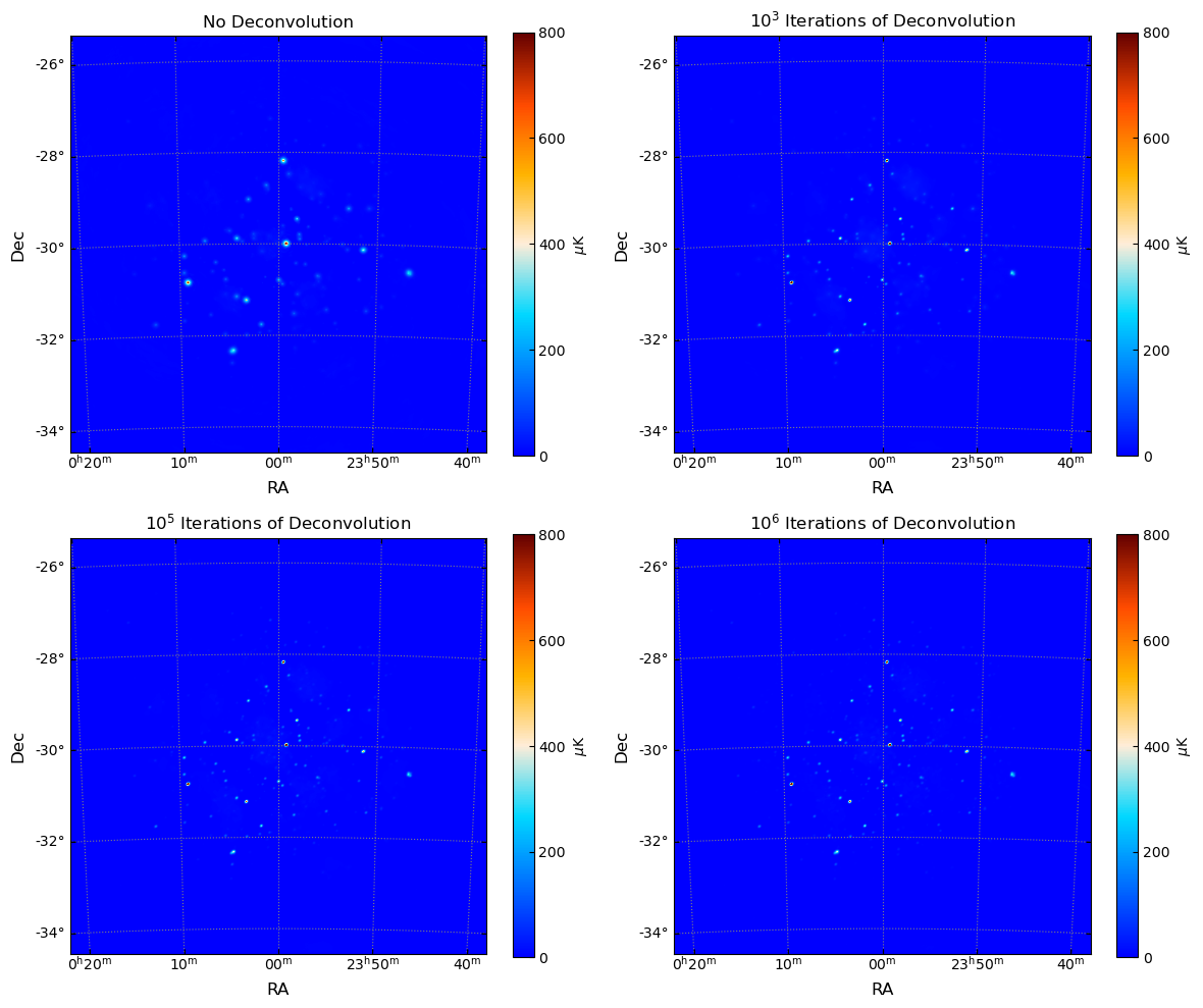
Figure 2: Deconvolved brightness temperature image at different iteration times, with a frequency of 166MHz. The upper left shows the case without deconvolution processing; the upper right image shows the deconvolution after 1000 iterations; the lower left image shows the deconvolution after 100,000 iterations; and the lower right image shows the deconvolution after 1,000,000 iterations. The units in the images are $\mu$K.

In data processing, the $\tt{CLEAN}$ method is a widely used technique for improving the quality of individual radio interferometric images. However, it does not produce a unique and stable solution and requires considerable computational resources. While the $\tt{CLEAN}$ algorithm is relatively easy to understand as a process for removing beam effects, it is a highly nonlinear method and does not provide a complete mathematical analysis.

When using the $\tt{WSClean}$ algorithm, several parameters must be manually chosen, such as selecting between natural weighting, uniform weighting, or Briggs weighting, which can affect the spatial resolution and noise level of the resulting image. The number of deconvolution iterations impacts the required computation time and result quality, with the number of iterations heavily relying on the user’s data processing experience. Other parameters include loop gain and window size. Additionally, the $\tt{WSClean}$ algorithm is known to introduce spurious structures such as scattered spots or wave-like features on extended source characteristics. To address these issues, we are exploring the use of deep learning algorithms.

3.2 PI-AstroDeconv Network and Training

This section provides a comprehensive description of the $\tt{PI-AstroDeconv}$ network architecture, including a detailed discussion on the selection of loss functions and training strategies.

3.2.1 PI-AstroDeconv Network

This subsection focuses on the network architecture. Our network is constructed based on the U-Net network structure, which was proposed by Ronneberger et al. to address the medical image segmentation problem (Ronneberger et al., 2015; Çiçek et al., 2016; Fabian & Klaus, 2019; Makinen et al., 2021; Ni et al., 2022). The U-Net network structure consists of symmetrical encoder and decoder components, where the encoder is used to extract high-level features of the image and the decoder is used to restore the feature maps to the original image size and perform segmentation. The core of the network is the U-shaped structure, which enables the network to capture both local and global information, resulting in more accurate segmentation. Since its inception, the U-Net network has been widely applied to various fields beyond segmentation problems, including regression problems. Specifically, the encoder is composed of multiple convolutional and pooling layers, which are used to extract high-level semantic features from the image. The decoder is composed of up-sampling layers and convolutional layers, which are used to restore the feature maps to the original image size and perform segmentation. In the decoder, each up-sampling layer is concatenated with the corresponding feature map in the encoder to exploit more abundant information. Furthermore, the U-Net network introduces skip connections, which connect a specific layer in the encoder to the corresponding layer in the decoder. The skip connections enable the decoder to utilize the high-level semantic information from the encoder without losing detail information, thereby enhancing the network’s expression ability and segmentation performance (Ronneberger et al., 2015).

In equation (4), the dirty beam is considered as a filter, playing the role of a convolutional kernel in deep learning . To illustrate this process more intuitively, we present a schematic diagram of the sky map convolution, as shown in Figure 3. The left side of the diagram displays the beam signal before convolution, the middle section shows the shape of the beam, and the right side depicts the blurring effect on the image caused by the PSF or beam, where the symbol “$\otimes$” represents the convolution operation, and “$=$” indicates the equivalence relationship.

Based on the aforementioned theory, we propose a physics-informed unsupervised learning method for astronomical image deconvolution, namely $\tt{PI-AstroDeconv}$, to effectively mitigate the beam effect. Furthermore, considering the substantial size of the dirty beam in aperture synthesis observations, we will investigate the strategy of replacing certain convolutional kernels in deep learning with Fast Fourier Transform (FFT) techniques to enhance processing efficiency.

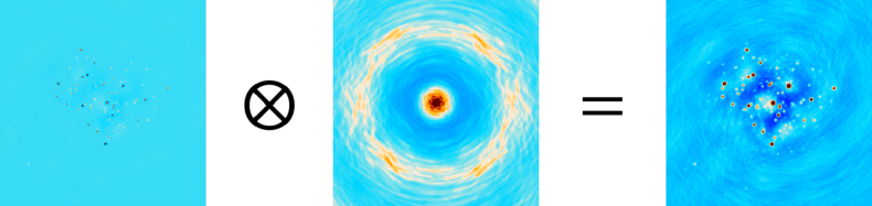
Figure 3: Schematic diagram of telescope observation effects. The image on the left displays the true, clean image of the observed target, while the image in the center reveals the shape of the telescope’s PSF or beam. The image on the right illustrates the blurring effect caused by the PSF or beam. The symbol “$\otimes$” denotes the convolution operation, and “$=$” is used to represent the equivalence relationship.

Our network has undergone some minor modifications on the basis of the U-Net network. A Depthwise convolutional layer is added between the U-Net and the output, and the convolution kernel of this layer is like the beam of a telescope. The input and label (Ground Truth) in the network are identical, which are observation data from a telescope, and the learning objective of the network is to output the same as the input. The final prediction of the network is the output of the U-Net before Depthwise convolution.

The architecture of $\tt{PI-AstroDeconv}$ is illustrated in Fig. 4. It consists of yellow blocks that depict convolutional layers, red blocks representing pooling layers, and gray-green blocks indicating upsampling operations. The left half of the network illustrates the downsampling path, while the right half represents the upsampling path. The number of channels is indicated at the bottom of each block, and the arrows above the image symbolize the connections between network layers. The numbers below each layer in the network denote the quantity of convolutional kernels present in that specific layer. Moreover, the letters indicate variations in image dimensions within the layer, with ”I” specifically denoting the size of the input image. The blocks on the far left and far right of the network represent the input and output, respectively, illustrated as deep blue circles. Between the U-Net network and the output, a depth convolutional layer appears as a yellow circle. This layer utilizes convolutional kernels resembling telescope beams and is accelerated using FFT. The network obtains the input and labels (Ground Truth) from telescope observations, with its objective being to produce the same information as the input. The network’s final prediction emerges from the last layer of the U-Net, represented as the last pink layer.

In actual astronomical observations, the dimensions of both the imaging and the telescope PSF are typically large. In order to preserve the integrity of the convolved images and PSF, we abstained from employing any segmentation and instead directly performed convolution calculations. However, the use of a large convolution kernel (2048x2048) in the final layer of the network hindered the learning process. To address this issue, we implemented a transformation technique that combines Fourier transform and convolution. More specifically, we replaced the convolution operation in the last layer with Fourier transform, resulting in a reduction of time complexity from $\mathcal{O}(n^{4})$ to $\mathcal{O}(n^{2}\times log(n))$ (Ni et al., 2024). We conducted comparative tests to evaluate the application effect of FFT acceleration in the training process. The results indicated that after enabling FFT acceleration, there was a significant reduction in processing time, especially for the large kernel convolution in the last layer of the network, with the improvement exceeding a factor of $10^{5}$.

Our objective is to eliminate the beam effects of telescopes through a network design that facilitates the use of data under known beam conditions, without the need for uncontaminated data as ground truth labels. Additionally, we can replace the U-Net (shown as the pink block in Figure 4 with any other network architecture and use the beam of any telescope (shown as the Beam block in Figure 4. Therefore, in a loose sense, our network can be considered a universal unsupervised network.

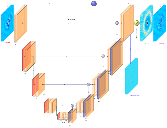
Figure 4: The $\tt{PI-AstroDeconv}$ architecture. The yellow blocks represent convolutional layers, red blocks represent pooling layers, and gray-green blocks represent upsampling operations. The left half of the network depicts the downsampling path, while the right half represents the upsampling path. The number of channels is indicated at the bottom of each block. The arrows above the image symbolize the connections between network layers. The numbers below each layer in the network indicate the quantity of convolutional kernels present in that specific layer. Additionally, the letters denote the variations in the image dimensions within the layer. The letter ”I” specifically represents the size of the input image. The blocks located at the far left and far right of the network indicate the input and output, respectively (represented as deep blue circles). A depth convolutional layer, represented by a yellow circle, is inserted between the U-Net network and the output. This layer utilizes convolutional kernels resembling telescope beams and is accelerated using FFT. The input and labels (Ground Truth) in the network are obtained from observations of the telescope, and the network’s objective is to output the same information as the input. The final prediction of the network is derived from the last layer of the U-Net, represented as the last pink layer. This visualization was created by modifying the PlotNeuralNet library (https://github.com/HarisIqbal88/PlotNeuralNet).

3.2.2 Loss Function

Our objective is to utilize supervised regression algorithms for the purpose of mitigating the adverse beam effects present in the data obtained from telescope observations. The $\tt{PI-AstroDeconv}$ algorithm employs input values to predict continuous outputs. When selecting a loss function, it is crucial to ensure the continuity and differentiability of the information. We have experimented with several regression loss functions, such as the mean absolute error (MAE) (L1 norm), mean squared error (MSE) (L2 norm), Huber, and Log-Cosh (Wang et al., 2020a).

Loss functions vary in continuity and differentiability. MAE is not differentiable at zero, leading to potential discontinuities in optimization. MSE is continuous and differentiable everywhere, with its derivative being twice the error, ensuring a smooth optimization process but is sensitive to outliers, risking overfitting. The Huber loss acts like MSE for small errors ($<\delta$) and MAE for larger errors, differentiable for small errors but not at $\delta$. Log-Cosh loss is continuous and twice-differentiable everywhere, with a derivative expressed as a function of error, providing a very smooth optimization process (Wang et al., 2020a).

Considering the robustness to outliers and the second-order differentiability offered by the Log-Cosh loss function, we lean towards regarding it as the optimal choice.

$$L(p,t)=\sum_{i}\log\cosh(p_{i}-t_{i}),$$ (6)

Log-Cosh is a logarithmic hyperbolic cosine loss function that calculates the logarithm of the hyperbolic cosine of the prediction error. In the case of minor losses, the Log-Cosh function exhibits similarities to the MAE function, whereas for substantial losses, it mirrors the MSE function while retaining its second-order differentiability. Conversely, the Huber loss function lacks differentiability in all scenarios. The MAE loss represents the average absolute error and solely considers the mean absolute distance between the predicted and expected data, rendering it incapable of addressing significant prediction errors. On the other hand, the MSE loss emphasizes crucial errors through squaring, thereby significantly influencing performance metrics. Thus, owing to the Log-Cosh function’s commendable robustness to outliers, we designate it as the most fitting approach.

3.2.3 Training and Testing Datasets

The core of our network training is the U-Net network (Ronneberger et al., 2015), which is a composition of a convolutional network and a deconvolutional network based on the fully convolutional network (FCN) (Long et al., 2015). Therefore, the convolutional layer serves as the vital element in these networks as it filters the input data.

According to the reaches of Makinen et al. (2021) and Ni et al. (2022), considering our GPU performance, we primarily focus on two sizes of convolutional kernels, $32$ and $16$, at the beginning of the input. The size of the convolutional kernel determines the field of view for convolution, and the sizes under consideration are $5\times 5$ and $3\times 3$. To achieve the desired output dimension, we employ “same” padding for both convolution and transpose convolution to manage the boundaries of the samples. The stride parameter determines the step size at which the convolutional kernel traverses the image. In our model, we preserve the default settings, where the convolutional stride is $1$ and the transpose convolution stride is $2$.

Table 2 demonstrates the specific hyperparameters used in the network. The analysis employed the Adam optimizer with standard TensorFlow parameters (Kingma & Ba, 2014; Reddi et al., 2019), and set $\beta_{1}=0.9$ and $\beta_{2}=0.999$. These hyperparameters were meticulously tuned to optimize the network. Ultimately, the optimal values for the initial number of convolutional filters, and batch size were set to $32$ and $2$, respectively. The total number of trainable parameters in this network is $7.4\times 10^{6}$, with a total of $9.04\times 10^{6}$ trainable parameters. Considering the presence of positive and negative values induced by temperature fluctuations in HI data, we selected the ReLU and LeakyReLU activation functions with an alpha value of 1.0 to address this relationship. Figure 6 illustrates the evolution of the loss function throughout the training process.

We employed four optimizers to implement the weight decay strategy, as illustrated in Table 2. The selected decay rate was determined as $10^{-5}$. Furthermore, considering the large dimensions of the images, we had to reduce the batch size to $2$ and $4$. In addition, we compared two optimizers and ultimately selected Adam as the preferred option. We trained for 20000 epochs using a piecewise constant decay learning rate. The specific learning rate decay is set as follows: $\mathbf{boundaries}=[1000,2000,4000,8000,14000]$; $\mathbf{values}=[0.1,0.01,0.001,0.0005,0.0001,0.00005]$. This means that the learning rate is $0.1$ for epochs $0\sim 1000$, $0.01$ for epochs $1000\sim 2000$, and so on. We conducted all the experiments using the TensorFlow2 on NVIDIA A40.

To provide a comprehensive comparison between the $\tt{CLEAN}$ algorithm and our $\tt{PI-AstroDeconv}$ algorithm, we have carefully presented five sets of images in Figure 5. Each set includes results from both algorithms, allowing for a clear and direct comparison of their differences and relative strengths.

As shown in Figure 6, the results processed by the $\tt{CLEAN}$ algorithm reveal that the point sources are significantly larger than those from $\tt{PI-AstroDeconv}$, accompanied by more pronounced cloud-like structures in their vicinities. To further evaluate the performance of these two algorithms, we will employ the $\tt{PCA}$ method for foreground subtraction, and subsequently conduct a comparative analysis of their performance based on this operation.

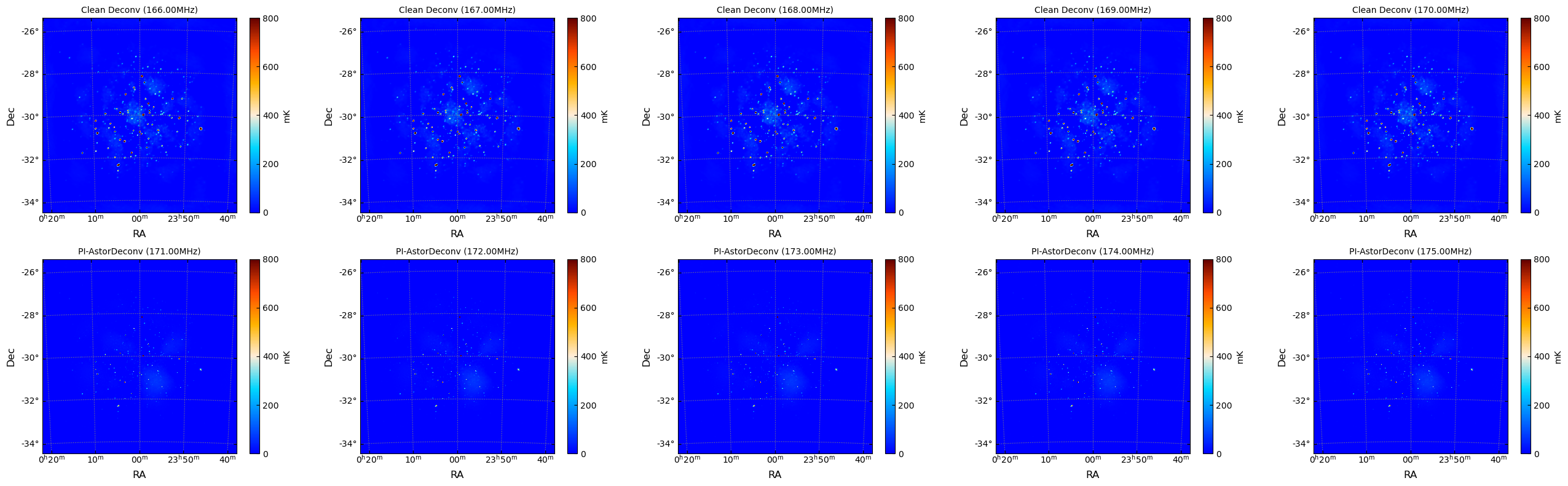
Figure 5: The top row of five images shows the results processed using the $\tt{CLEAN}$ algorithm, with frequencies from left to right being $166$ MHz, $167$ MHz, $168$ MHz, $169$ MHz, and $170$ MHz, respectively. Each image underwent $10^{6}$ iterations of deconvolution. The bottom row presents the deconvolution results obtained using the $\tt{PI-AstroDeconv}$ algorithm, with frequencies consistent with those in the top row. Each image in this row was directly input into the $\tt{PI-AstroDeconv}$ network without prior deconvolution using the $\tt{CLEAN}$ algorithm.

Table 2: Description of the hyperparameters in the U-Net architecture design.

Hyperparameter	Description	Prior Values	Optimum Value
$\omega$	weight decay for optimizer	[$10^{-4},10^{-5},10^{-6},10^{-7}$]	$10^{-5}$
$n_{\rm filters}$	initial number of convolution filters	[16, 32]	32
$b$	batch size, i.e. number of samples per gradient descent step	[1, 2]	4
$\Omega$	optimizer for training	[Adam, NAdam]	NAdam

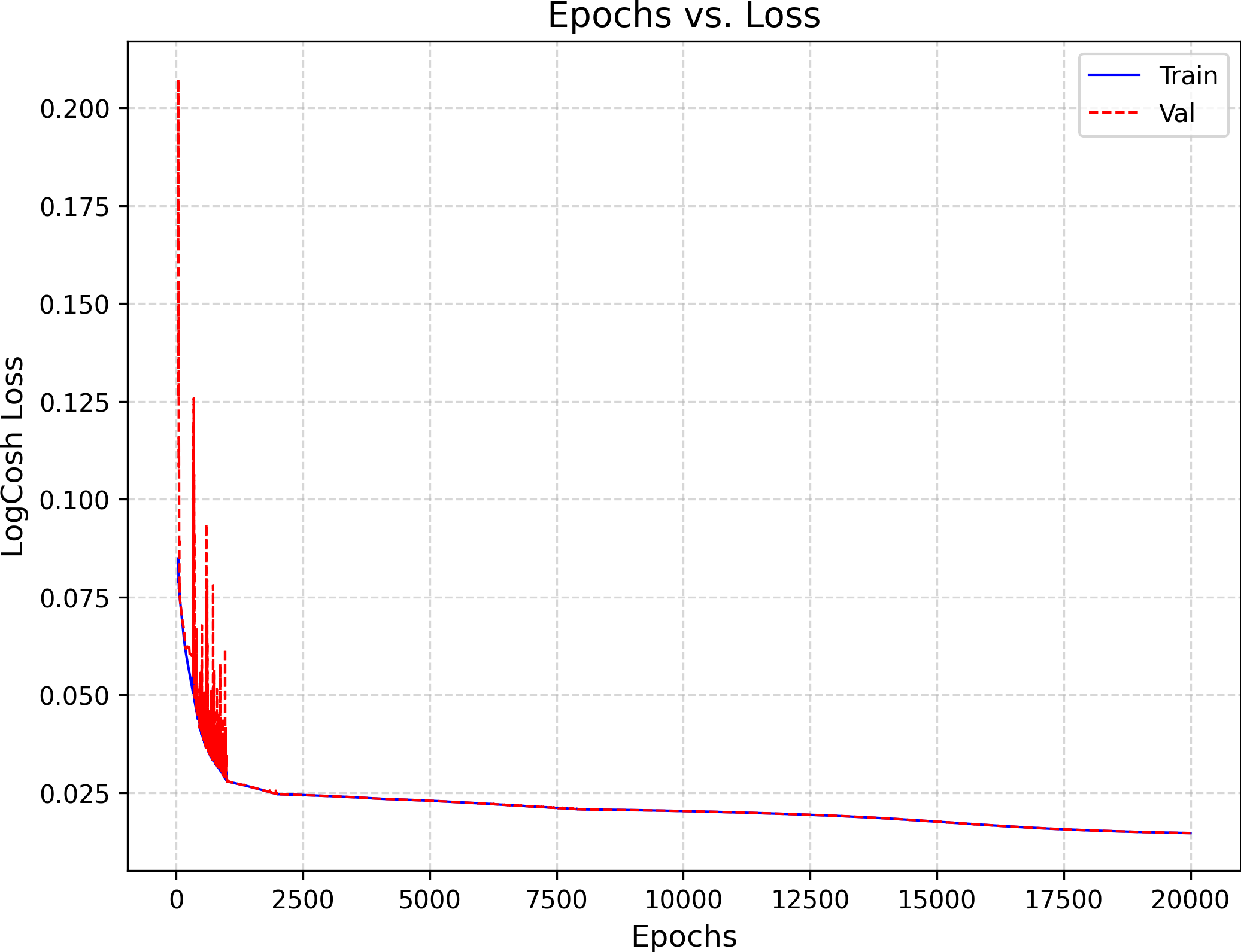
Figure 6: Loss function evolution for each network as a function of the number of epochs. The dark blue solid line indicates the training set loss function evolution and the red dashed line indicates the validation set loss function evolution.

4 Results and Discussion

In the previous chapter, we explored in-depth the techniques of interferometric imaging, traditional deconvolution algorithms, and deep learning-based deconvolution methods. In this section, we will conduct a comprehensive and detailed analysis of two-dimensional matter power spectra of the obtained results.

4.1 PCA Foreground Subtraction

$\tt{PCA}$ (Principal Component Analysis) is a widely used statistical technique for dimensionality reduction and feature extraction. Its core mechanism involves identifying and retaining the principal directions of variance within the data, known as principal components. By performing an orthogonal transformation, $\tt{PCA}$ maps the original data to a new coordinate system where the variance is maximized. When dealing with 21 cm hydrogen line data, foreground signals often exhibit smooth variations across multiple frequency bands, whereas cosmic background signals primarily manifest as variations on larger spatial scales. By calculating the covariance matrix and performing eigenvalue decomposition, $\tt{PCA}$ can effectively identify dominant patterns associated with foreground signals and subsequently remove these patterns from the observational data (de Oliveira-Costa et al., 2008; Alonso et al., 2015; Makinen et al., 2021). Consequently, $\tt{PCA}$ is frequently employed as a key tool in the foreground removal analysis for neutral hydrogen (HI), enabling the extraction of the cosmic HI signal by stripping away foreground interference from complex astronomical images.

The advantage of this method is that it does not require prior knowledge of the specific form of the foreground, making it an effective blind noise reduction technique. However, since the cosmic signal may also exhibit smooth structures on large scales, $\tt{PCA}$ might remove cosmological clustering information valuable for research. Therefore, when applying $\tt{PCA}$ to remove foregrounds, it is necessary to carefully select the number of principal components to remove, in order to balance the trade-off between noise reduction and the preservation of useful signals.

In another study, we learned that the beam effect can significantly influence the performance of the $\tt{PCA}$ algorithm in removing the neutral hydrogen foreground. Therefore, in this research, we first subjected the data to visualization processes and obtained results through imaging. Subsequently, we selected two deconvolution methods for comparison: the traditional algorithm and the $\tt{PI-AstroDeConv}$ algorithm. The adoption of the advanced deconvolution method stems from the fact that the beam effect of the interferometer array can impact the efficacy of $\tt{PCA}$. Our ultimate goal is to compare the performance of the traditional algorithm and the $\tt{PI-AstroDeConv}$ algorithm in mitigating the beam effect.

4.2 Matter Power Spectrum Analysis

To ensure that the correction of the beam effect during the data analysis process did not compromise the authenticity of the cosmic matter distribution, we conducted a 2-D matter power spectrum analysis on the processed data. By thoroughly analyzing the matter power spectrum, we can assess the effectiveness of the beam effect correction and determine whether crucial physical information has been preserved.

The 2-D Power Spectrum is a statistical tool used to measure the spatial correlation of HI in two different directions. Specifically, it focuses on the distribution of HI parallel to the line of sight ($k_{\parallel}$) and perpendicular to the line of sight ($k_{\perp}$). By analyzing the 2D Power Spectrum of HI, scientists can investigate the early state of the universe, which is one of the objectives of the SDC3a project, namely, to probe the EoR of the universe through observations of the 21-cm line. Additionally, the 2D Power Spectrum of HI can also be used to study the distribution patterns of galaxies and galaxy clusters in the universe, revealing the characteristics of HI gas distribution within galactic disks. Since the distribution of HI is influenced by the gravitational potential of dark matter, the analysis of the power spectrum allows for the indirect detection and study of the properties of dark matter.

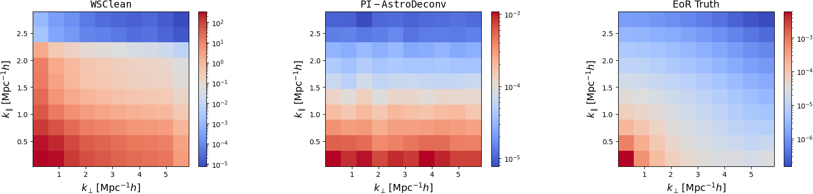
Figure 7: The 2D matter power spectrum ratio of the PCA cleaned map. The left panel displays the residuals after correcting the beam effect using $\tt{WSClean}$ and removing the foreground contamination through the PCA algorithm. The middle panel reflects the residuals after correcting the beam effect with the $\tt{PI-AstroDeconv}$ algorithm and similarly removing the foreground influence via the $\tt{PCA}$ method. The right panel presents the true power spectrum of the EoR.

In Figure 7, we present the two-dimensional matter power spectrum. The left panel displays the true power spectrum obtained from the SDC3a project, while the center panel shows the power spectrum predicted by the $\tt{PI-AstroDeconv}$ algorithm.

Analysis of the discrepancy plot reveals that the power spectra corresponding to small $k_{\perp}$ and large $k_{\parallel}$, as well as those corresponding to large $k_{\perp}$ and small $k_{\parallel}$, exhibit relatively larger differences compared to other positions. Nonetheless, overall, the differences between the predicted power spectrum and the true power spectrum are relatively minor and are generally kept within a range of $3\%$.

To facilitate a direct comparison between the two, we have constructed the right panel based on Equation (7), which highlights the differences.

$$R(k_{\parallel},k_{\perp})=\frac{P_{\rm pred}(k_{\parallel},k_{\perp})}{P_{\rm truth}(k_{\parallel},k_{\perp})}-1,$$ (7)

where $P_{\rm pred}(k_{\parallel},k_{\perp})$ is the predicted power spectrum predicted, and $P_{\rm truth}(k_{\parallel},k_{\perp})$ is the truth power spectrum.

In Equation (7), the parameter $R(k_{\parallel},k_{\perp})$ serves to effectively delineate the extent of the discrepancy between actual observations and model forecasts. However, to more intuitively illustrate these differences, we have simplified the quantification process, as detailed in the following formula:

$$\Gamma={\rm mean}\left\{R(k_{\parallel},k_{\perp})_{\rm X}\right\}+1,$$ (8)

where the notation ${\rm mean}\{\}$ is used to denote the operation of calculating the average of the parameter $R(k_{\parallel},k_{\perp})$. Through our calculations, we obtained a result of $\Gamma=0.03190$, which demonstrates that the method we utilized has effectively achieved beam mitigation to a notable degree.

5 Conclusion

In the field of astronomy, beam effects are image distortions caused by factors such as the optical characteristics of telescopes and observation conditions, posing challenges for precise cosmic observations and research. Traditional beam correction methods rely on accurate physical models and complex algorithms, which often require extensive prior knowledge and manual intervention, and may struggle to adapt to unknown or variable observation conditions.

Proposing a deep learning-based unsupervised algorithm to remove beam effects from astronomical images is of revolutionary significance. Firstly, unsupervised learning algorithms can directly learn the characteristics of beam effects from unmarked observational data without relying on precise physical models, greatly expanding the applicability of the algorithm. Secondly, the powerful representational capabilities of deep learning models enable them to capture complex nonlinear relationships, thereby more effectively removing beam effects and restoring the true appearance of celestial images.

Furthermore, the use of unsupervised algorithms reduces reliance on expert knowledge, making astronomical data processing more efficient and automated. This is particularly important for the rapid processing and real-time analysis of astronomical observation data, especially when dealing with large volumes of data, such as that obtained from large-scale sky surveys. At the same time, the generalization capability of this method means that once the model is trained, it can be applied to data from different telescopes and under various observation conditions, improving the efficiency of resource utilization.

More importantly, an unsupervised algorithm based on deep learning to remove beam effects can significantly enhance the quality of astronomical observation data, providing astronomers with clearer images of the cosmos. This not only aids in more accurate measurements of celestial physical parameters, such as the brightness of stars and the shape of galaxies, but also reveals previously unrecognized astronomical phenomena, promoting new scientific discoveries.

Data Availability

References

- Aghanim et al. (2020) Aghanim, N., et al. 2020, Astron. Astrophys., 641, A6, doi: 10.1051/0004-6361/201833910
- Alexander et al. (2011) Alexander, P., Bregman, J. A., & Faulkner, A. J. 2011, PoS, SKADS 2009, 016, doi: 10.22323/1.132.0016
- Alonso et al. (2015) Alonso, D., Bull, P., Ferreira, P. G., & Santos, M. G. 2015, Mon. Not. Roy. Astron. Soc., 447, 400, doi: 10.1093/mnras/stu2474
- An et al. (2019) An, Y., Li, J., Huang, L., et al. 2019, Optics Express, 27, 18683
- Bacon et al. (2020) Bacon, D. J., et al. 2020, Publ. Astron. Soc. Austral., 37, e007, doi: 10.1017/pasa.2019.51
- Bandura et al. (2014) Bandura, K., et al. 2014, Proc. SPIE Int. Soc. Opt. Eng., 9145, 22, doi: 10.1117/12.2054950
- Bean et al. (2022) Bean, B., et al. 2022, Publ. Astron. Soc. Pac., 134, 114501, doi: 10.1088/1538-3873/ac9642
- Bull et al. (2015) Bull, P., Ferreira, P. G., Patel, P., & Santos, M. G. 2015, Astrophys. J., 803, 21, doi: 10.1088/0004-637X/803/1/21
- Burns et al. (2012) Burns, J. O., Lazio, J., Bale, S., et al. 2012, Advances in Space Research, 49, 433
- Camilo et al. (2018) Camilo, F., et al. 2018, Astrophys. J., 856, 180, doi: 10.3847/1538-4357/aab35a
- Chiche et al. (2023) Chiche, B. N., Girard, J. N., Frontera-Pons, J., Woiselle, A., & Starck, J.-L. 2023, Astronomy & Astrophysics, 675, A116
- Clark (1980) Clark, B. 1980, Astronomy and Astrophysics, vol. 89, no. 3, Sept. 1980, p. 377, 378., 89, 377
- Collaboration et al. (2018) Collaboration, T. C., Amiri, M., Bandura, K., et al. 2018, The Astrophysical Journal, 863, 48, doi: 10.3847/1538-4357/aad188
- Cornwell (1983) Cornwell, T. 1983, Astronomy and Astrophysics (ISSN 0004-6361), vol. 121, no. 2, May 1983, p. 281-285., 121, 281
- Cornwell (2008) Cornwell, T. J. 2008, IEEE Journal of selected topics in signal processing, 2, 793
- Cornwell (2009) —. 2009, Geochem. Geophys. Geosyst., 10, 9U07, doi: 10.1029/2009GC002604
- Davis et al. (1985) Davis, M., Efstathiou, G., Frenk, C. S., & White, S. D. 1985, Astrophysical Journal, Part 1 (ISSN 0004-637X), vol. 292, May 15, 1985, p. 371-394. Research supported by the Science and Engineering Research Council of England and NASA., 292, 371
- de Bernardis et al. (2000) de Bernardis, P., et al. 2000, Nature, 404, 955, doi: 10.1038/35010035
- de Oliveira-Costa et al. (2008) de Oliveira-Costa, A., Tegmark, M., Gaensler, B. M., et al. 2008, Mon. Not. Roy. Astron. Soc., 388, 247, doi: 10.1111/j.1365-2966.2008.13376.x
- de Vos et al. (2009) de Vos, M., Gunst, A. W., & Nijboer, R. 2009, Proceedings of the IEEE, 97, 1431, doi: 10.1109/JPROC.2009.2020509
- Dewdney et al. (2017) Dewdney, P. E., Braun, R., & Turner, W. 2017, in 2017 XXXIInd General Assembly and Scientific Symposium of the International Union of Radio Science (URSI GASS), 1–4, doi: 10.23919/URSIGASS.2017.8105425
- Dodson et al. (2022) Dodson, R., Momjian, E., Pisano, D. J., et al. 2022, The Astronomical Journal, 163, 59, doi: 10.3847/1538-3881/ac3e65
- Drake & Sagan (1973) Drake, F. D., & Sagan, C. 1973, Nature, 245, 257
- Fabian & Klaus (2019) Fabian, I., & Klaus, M.-H. 2019, arXiv e-prints, arXiv:1908.02182. https://arxiv.org/abs/1908.02182
- Gao et al. (2023) Gao, L.-Y., Li, Y., Ni, S., & Zhang, X. 2023, Mon. Not. Roy. Astron. Soc., 525, 5278, doi: 10.1093/mnras/stad2646
- Gudel (2002) Gudel, M. 2002, Ann. Rev. Astron. Astrophys., 40, 217, doi: 10.1146/annurev.astro.40.060401.093806
- Hamaker (2006) Hamaker, J. 2006, Astronomy & Astrophysics, 456, 395
- Hjellming (1989) Hjellming, R. 1989, in Synthesis Imaging in Radio Astronomy, Vol. 6, 477
- Högbom (1974) Högbom, J. 1974, Astronomy and Astrophysics Supplement, Vol. 15, p. 417, 15, 417
- Hogbom (1974) Hogbom, J. A. 1974, Astron. Astrophys. Suppl. Ser., 15, 417
- Jelic et al. (2008) Jelic, V., et al. 2008, Mon. Not. Roy. Astron. Soc., 389, 1319, doi: 10.1111/j.1365-2966.2008.13634.x
- Johnston & Wall (2008) Johnston, S., & Wall, J. 2008, Exper. Astron., 22, 151, doi: 10.1007/s10686-008-9124-7
- Johnston et al. (2007) Johnston, S., et al. 2007, PoS, MRU, 006, doi: 10.1071/AS07033
- Kellermann et al. (2020) Kellermann, K. I., Bouton, E. N., & Brandt, S. S. 2020, Open skies: The national radio astronomy observatory and its impact on US radio astronomy (Springer Nature), 319–390. https://doi.org/10.1007/978-3-030-32345-5_7
- Kingma & Ba (2014) Kingma, D. P., & Ba, J. 2014, CoRR, abs/1412.6980. https://api.semanticscholar.org/CorpusID:6628106
- Li et al. (2012) Li, D., Nan, R., & Pan, Z. 2012, Proceedings of the International Astronomical Union, 8, 325–330, doi: 10.1017/S1743921312024015
- Li et al. (2018) Li, D., Wang, P., Qian, L., et al. 2018, IEEE Microwave Magazine, 19, 112, doi: 10.1109/MMM.2018.2802178
- Long et al. (2015) Long, J., Shelhamer, E., & Darrell, T. 2015, in Proceedings of the IEEE conference on computer vision and pattern recognition, 3431–3440
- Lonsdale et al. (2009) Lonsdale, C. J., Cappallo, R. J., Morales, M. F., et al. 2009, Proceedings of the IEEE, 97, 1497, doi: 10.1109/JPROC.2009.2017564
- Lucherini et al. (2021) Lucherini, E., Sun, M., Winecoff, A. A., & Narayanan, A. 2021, ArXiv, abs/2107.08959. https://api.semanticscholar.org/CorpusID:236087868
- Lynch et al. (2021) Lynch, C., Galvin, T., Line, J., et al. 2021, arXiv preprint arXiv:2110.08400
- Makinen et al. (2021) Makinen, T. L., Lancaster, L., Villaescusa-Navarro, F., et al. 2021, JCAP, 04, 081, doi: 10.1088/1475-7516/2021/04/081
- Martin & Irvine (1983) Martin, B. R., & Irvine, J. 1983, Research Policy, 12, 61, doi: https://doi.org/10.1016/0048-7333(83)90005-7
- Mathews (2013) Mathews, J. D. 2013, History of Geo- and Space Sciences, 4, 19, doi: 10.5194/hgss-4-19-2013
- Mesinger et al. (2011) Mesinger, A., Furlanetto, S., & Cen, R. 2011, Mon. Not. Roy. Astron. Soc., 411, 955, doi: 10.1111/j.1365-2966.2010.17731.x
- Mort et al. (2016) Mort, B., Dulwich, F., Razavi-Ghods, N., de Lera Acedo, E., & Grainge, K. 2016, Monthly Notices of the Royal Astronomical Society, stw2814
- Mort et al. (2010) Mort, B. J., Dulwich, F., Salvini, S., Adami, K. Z., & Jones, M. E. 2010, in 2010 IEEE International Symposium on Phased Array Systems and Technology, IEEE, 690–694
- Muñoz et al. (2022) Muñoz, J. B., Qin, Y., Mesinger, A., et al. 2022, Mon. Not. Roy. Astron. Soc., 511, 3657, doi: 10.1093/mnras/stac185
- Murray et al. (2020) Murray, S. G., Greig, B., Mesinger, A., et al. 2020, J. Open Source Softw., 5, 2582, doi: 10.21105/joss.02582
- Nan et al. (2011) Nan, R., Li, D., Jin, C., et al. 2011, Int. J. Mod. Phys. D, 20, 989, doi: 10.1142/S0218271811019335
- Napier et al. (1983) Napier, P. J., Thompson, A. R., & Ekers, R. D. 1983, Proceedings of the IEEE, 71, 1295
- Ni et al. (2022) Ni, S., Li, Y., Gao, L.-Y., & Zhang, X. 2022, Astrophys. J., 934, 83, doi: 10.3847/1538-4357/ac7a34
- Ni et al. (2024) Ni, S., Qiu, Y., Chen, Y., et al. 2024, arXiv preprint arXiv:2403.01692
- Offringa et al. (2014) Offringa, A. R., McKinley, B., Hurley-Walker, et al. 2014, MNRAS, 444, 606, doi: 10.1093/mnras/stu1368
- Offringa & Smirnov (2017) Offringa, A. R., & Smirnov, O. 2017, MNRAS, 471, 301, doi: 10.1093/mnras/stx1547
- Park et al. (2019) Park, J., Mesinger, A., Greig, B., & Gillet, N. 2019, Mon. Not. Roy. Astron. Soc., 484, 933, doi: 10.1093/mnras/stz032
- Perley et al. (2011) Perley, R., Chandler, C., Butler, B., & Wrobel, J. 2011, The Astrophysical Journal Letters, 739, L1
- Reddi et al. (2019) Reddi, S. J., Kale, S., & Kumar, S. 2019, CoRR, abs/1904.09237
- Rich et al. (2008) Rich, J. W., de Blok, W. J. G., Cornwell, T. J., et al. 2008, Astron. J., 136, 2897, doi: 10.1088/0004-6256/136/6/2897
- Rohlfs & Wilson (2013) Rohlfs, K., & Wilson, T. L. 2013, Tools of radio astronomy (Springer Science & Business Media)
- Ronneberger et al. (2015) Ronneberger, O., Fischer, P., & Brox, T. 2015, arXiv e-prints, arXiv:1505.04597. https://arxiv.org/abs/1505.04597
- Röttgering (2003) Röttgering, H. 2003, New Astronomy Reviews, 47, 405, doi: https://doi.org/10.1016/S1387-6473(03)00057-5
- Santos et al. (2015) Santos, M. G., et al. 2015, PoS, AASKA14, 019, doi: 10.22323/1.215.0019
- Sault et al. (1995) Sault, R. J., Teuben, P. J., & Wright, M. C. H. 1995, ASP Conf. Ser., 77, 433. https://arxiv.org/abs/astro-ph/0612759
- Schmidt et al. (2022) Schmidt, K., Geyer, F., Fröse, S., et al. 2022, Astronomy & Astrophysics, 664, A134
- Schwab (1984) Schwab, F. 1984, Astronomical Journal (ISSN 0004-6256), vol. 89, July 1984, p. 1076-1081., 89, 1076
- Schwab & Cotton (1983) Schwab, F. R., & Cotton, W. D. 1983, Astronomical Journal (ISSN 0004-6256), vol. 88, May 1983, p. 688-694., 88, 688
- Sorgho et al. (2018) Sorgho, A., Carignan, C., Pisano, D. J., et al. 2018, Monthly Notices of the Royal Astronomical Society, 482, 1248, doi: 10.1093/mnras/sty2785
- Spinelli et al. (2021) Spinelli, M., Carucci, I. P., Cunnington, S., et al. 2021, Mon. Not. Roy. Astron. Soc., 509, 2048, doi: 10.1093/mnras/stab3064
- Springel et al. (2006) Springel, V., Frenk, C. S., & White, S. D. M. 2006, Nature, 440, 1137, doi: 10.1038/nature04805
- The Staff at the National Astronomy and Ionosphere Center (1975) The Staff at the National Astronomy and Ionosphere Center. 1975, Icarus, 26, 462, doi: https://doi.org/10.1016/0019-1035(75)90116-5
- Thompson et al. (2017a) Thompson, A. R., Moran, J. M., & Swenson, G. W. 2017a, Interferometry and synthesis in radio astronomy (Springer Nature)
- Thompson et al. (2017b) —. 2017b, Interferometry and synthesis in radio astronomy (Springer Nature)
- Tingay et al. (2013) Tingay, S. J., Goeke, R., Bowman, J. D., et al. 2013, Publications of the Astronomical Society of Australia, 30, e007, doi: 10.1017/pasa.2012.007
- Van der Tol et al. (2018) Van der Tol, S., Veenboer, B., & Offringa, A. R. 2018, A&A, 616, A27, doi: 10.1051/0004-6361/201832858
- Vermeulen & van Haarlem (2011) Vermeulen, R. C., & van Haarlem, M. 2011, in 2011 XXXth URSI General Assembly and Scientific Symposium, 1–1, doi: 10.1109/URSIGASS.2011.6051244
- Wakker & Schwarz (1988) Wakker, B. P., & Schwarz, U. 1988, Astronomy and Astrophysics (ISSN 0004-6361), vol. 200, no. 1-2, July 1988, p. 312-322. Research supported by ZWO., 200, 312
- Wang et al. (2020a) Wang, Q., Ma, Y., Zhao, K., & Tian, Y. 2020a, Annals of Data Science, 1
- Wang et al. (2020b) Wang, R., Wicenec, A., & An, T. 2020b, Sci. Bull., 65, 337, doi: 10.1016/j.scib.2019.12.016
- Wayth et al. (2015) Wayth, R. B., et al. 2015, Publ. Astron. Soc. Austral., 32, e025, doi: 10.1017/pasa.2015.26
- Williamson et al. (2021) Williamson, A., James, C., Tingay, S., Bray, J., & Huege, T. 2021, PoS, ICRC2021, 325, doi: 10.22323/1.395.0325
- Wilson et al. (2009) Wilson, T. L., Rohlfs, K., & Hüttemeister, S. 2009, Interferometers and Aperture Synthesis (Berlin, Heidelberg: Springer Berlin Heidelberg), 201–237, doi: 10.1007/978-3-540-85122-6_9
- WU et al. (2015) WU, M., CAO, R., Tao, X., et al. 2015, Scientia Sinica Informationis, 45, 1600, doi: 10.1360/N112015-00132
- Zheng et al. (2017) Zheng, H., Tegmark, M., Dillon, J. S., et al. 2017, Mon. Not. Roy. Astron. Soc., 464, 3486, doi: 10.1093/mnras/stw2525
- Çiçek et al. (2016) Çiçek, Ö., Abdulkadir, A., Lienkamp, S. S., Brox, T., & Ronneberger, O. 2016, arXiv e-prints, arXiv:1606.06650. https://arxiv.org/abs/1606.06650