Analyzing and Forecasting the Success in the Men’s Ice Hockey World (Junior) Championships Using a Dynamic Ranking Model

Abstract: What factors contribute to the success of national teams in the Men’s Ice Hockey World Championships and the Men’s Ice Hockey World Junior Championships? This study examines whether hosting the tournament provides a home advantage; the influence of past tournament performances; the impact of players’ physical characteristics such as height, weight, and age; and the value of experience from the World Championships compared to the NHL and other leagues. We employ a dynamic ranking model based on the Plackett–Luce distribution with time-varying strength parameters driven by the score. Additionally, we conduct a forecasting analysis to predict the probabilities of winning the tournament, earning a medal, and advancing to the playoff phase.

Keywords: Ice Hockey, World Championships, World Junior Championships, Ranking Data, Plackett–Luce Distribution, Score-Driven Model.

JEL Codes: C23, C25, L83, Z21.

1 Introduction

The Men’s Ice Hockey World Championships (WC) are annual international tournaments organized by the International Ice Hockey Federation (IIHF). They are among the most prestigious events in the sport of ice hockey and feature national teams from around the world competing for the title of world champion. The IIHF also organizes the Men’s Ice Hockey World Junior Championships (WJC) for players under 20 years old. This paper focuses on a statistical analysis of the results from both of these tournaments.

In the field of sports statistics, ice hockey has been analyzed from various perspectives. The existing literature predominantly covers the National Hockey League (NHL), but other leagues are occasionally analyzed as well. For example, Leard and Doyle (2011) utilized a probit model to analyze NHL games and found evidence of home advantage and game-to-game momentum, but no link between winning fights and winning games. Doyle and Leard (2012) further focused on the sources of home advantage in the NHL using a panel regression on season-level data and a probit model on game-level data. Guérette et al. (2021) modeled the number of awarded penalties and found that NHL referees favored the home team when spectators were present. Thrane (2023) conducted a similar study for the Norwegian league and found that there is a home advantage in the presence of spectators. Marek et al. (2014) modeled and predicted the outcomes of games in the Czech league using the bivariate Poisson distribution with exponentially weighted observations. Whelan and Klein (2021) studied and extended the Bradley–Terry model in the context of ice hockey. Buttrey et al. (2011) estimated the rates at which NHL teams score and concede goals. Gu et al. (2019) developed a machine learning system to predict the outcomes of NHL games. Schulte et al. (2017) utilized the Markov game framework to evaluate player actions, locations, and team performance in the NHL. MacDonald (2011) developed an adjusted plus-minus statistic to quantify the overall contribution of NHL players to their teams. Tarter et al. (2009) evaluated the long-term value of elite junior ice hockey players to their future NHL teams. Von Allmen et al. (2015) examined wage premia for European players in the NHL.

These studies mostly focus on the outcomes of individual matches or specific partial statistics. The study of Holý and Zouhar (2022), however, offers a notable exception by modeling the final standings, i.e., the complete ranking of all participating teams. Prior to the work of Holý and Zouhar (2022), a review of the ranking literature by Yu et al. (2019) highlighted the lack of dynamics in existing ranking models. Addressing this gap, Holý and Zouhar (2022) proposed a score-driven model based on the Plackett–Luce distribution, offering a universally applicable time series approach for rankings. This model was applied to the results of the Men’s Ice Hockey World Championships. However, the application was more illustrative than in-depth, and the approach was purely time-series-based and incorporated only a single predictor variable: a dummy variable indicating the host country, which was ultimately found to be insignificant in the analysis.

This paper aims to build upon and extend the study of Holý and Zouhar (2022) by incorporating a broader range of predictor variables. In addition to focusing on the World Championships, we also examine the World Junior Championships and explore the relation between the two. Our first objective is to evaluate the impact of factors such as the results from related tournaments, players’ physical attributes, and players’ experience on the success of national teams. The inclusion of these variables necessitates several modifications to the model proposed by Holý and Zouhar (2022). Consequently, we introduce a novel ranking model that features separate regression and dynamic components and can handle non-participating teams. Our second objective is to assess the forecasting performance of our approach. Since our main focus is on the ranking, the model naturally provides predictions for various derived probabilities, such as the likelihood of winning the tournament, earning a medal, or advancing to the playoff phase.

Among the key questions we seek to answer are: Do national teams exhibit stable strength levels over the long term, or do their strengths evolve more rapidly? Does the hosting team enjoy a home advantage? Does success in the World Junior Championship translate into success in the next World Championship? Similarly, does success in the World Under-18 Championship translate into success in the next World Junior Championship? Do overall physical characteristics, such as average height and weight, significantly impact performance? Is it advantageous to have a younger team in the World Championships? Is experience from the World Championships more valuable than experience from the NHL? Are there notable differences in the factors influencing performance in the World Junior Championships compared to the World Championships? How accurately can the results of the tournaments be predicted?

The remainder of the paper is structured as follows: In Section 2, we highlight the specifics of the WC and WJC and present the analyzed dataset. In Section 3, we propose our dynamic ranking model and describe the methods of its estimation. In Section 4, we report the results of the analysis and discuss their implications. We conclude the paper in Section 5.

2 Background

2.1 World Championships and Other Tournaments

The Men’s Ice Hockey World Championships were first officially held during the 1920 Summer Olympics. In 1930, the first championship separate from the Olympics took place. These championships continued to be held annually, with the Olympic hockey tournaments serving as the World Championships for those years until 1968. Since 1972, the World Championships have been held independently, even in Olympic years. During the three Winter Olympics in the 80s, however, the World Championships were not held. The tournament was also not held from 1940 to 1946 due to World War II. Recently, the 2020 tournament was canceled due to the COVID-19 pandemic. The 2024 tournament marked the 87th edition.

Currently, the World Championships feature 16 teams. The preliminary round consists of two groups, with seedings determined by the IIHF World Ranking. Each group includes 8 teams competing in a round-robin format, with the top 4 teams from each group advancing to the playoff round. This round begins with four quarter-final matches, and the four winning teams progress to the semi-finals. The tournament concludes with the final match and the third-place game. The final standings represent the complete ranking of all 16 participating teams. The ranks of the top 4 teams are determined by the playoffs, while the ranks of the remaining teams are primarily determined by the points earned from the matches in the preliminary round and the quarter-finals. The final standings are used to update the IIHF World Ranking. In addition to this Top Division, the tournament features lower-tier Divisions I through IV. The bottom two teams from the Top Division are relegated to Division I for the following year, while the top two teams from Division I are promoted to the Top Division.

The World Championships, along with the Olympic ice hockey tournament (also governed by the IIHF), are considered the most prestigious international ice hockey tournaments. The NHL, on the other hand, is the premier professional ice hockey league in North America and features many of the world’s best players. While the World Championships and the Olympic tournament highlight international competition among national teams, the NHL represents the highest level of club competition in the world. The World Championships are typically held in May, following the NHL regular season but during the NHL playoffs. Consequently, some top NHL players are unable to participate in the World Championships due to NHL commitments or injuries. Some characteristics of both tournaments are listed in Table 1. The two tournaments also differ in the size and shape of the rinks, as well as in some specific rules.

The World Championships are dominated by the so-called Big Six teams: Canada and the United States from North America, and Czechia, Finland, Russia, and Sweden from Europe. The Big Six teams collectively won 85 gold medals, while the World Championships were won by another team only twice. The Czechia team is the successor to the Czechoslovakia team, which disbanded in 1992. At the same time, the Slovakia team also emerged, starting international play in the lowest pool and advancing to the top pool by 1996. The Russia team is the successor to the Soviet Union team, which disbanded in 1991, and briefly competed as the Commonwealth of Independent States (CIS) team. Following the dissolution of the Soviet Union; Belarus, Kazakhstan, Latvia, and Ukraine, among others, established their own national teams. The modern Germany team emerged after the unification of the West and East German teams in 1991 and is considered the successor to West Germany. In this paper, we consider Czechoslovakia/Czechia, the Soviet Union/CIS/Russia, and West Germany/Germany as single teams, referring to them by their latest designation. Other teams regularly participating in the World Championships include Austria, Denmark, France, Italy, Norway, Slovenia, and Switzerland. Occasionally, teams from Great Britain, Hungary, Japan, and Poland also participate.

Each year, a different country hosts the World Championships. The most frequent host countries are Czechia and Sweden, each having hosted 11 times, followed by Finland and Switzerland, each having hosted 10 times. Occasionally, the hosting is shared between two or even three countries. The World Championships have been hosted outside Europe only four times: once in Canada and three times in the United States. It is evident that the tournament is popular in Europe, while North America prioritizes the NHL. This is especially true for the United States, which often uses the World Championships as an opportunity to give experience to younger players.

The IIHF also organizes tournaments for younger men. From 1974 to 1976, three unofficial junior tournaments were held for players under 20. Since 1977, the official Men’s World Junior Championships, also known as the Men’s World Under-20 Championships, has been held by the IIHF. The 2024 tournament marked the 48th edition. The WJC tournament usually takes place at the turn of December and January. The WJC tournament is especially popular in Canada, which has hosted it 17 times. For even younger players, there is the Men’s World Under-18 Championships (U18). The tournament started in 1999, and the 2024 edition marked its 25th iteration. The U18 tournament usually takes place at April. The U18 tournament is dominated by the United States, which has won 11 out of 25 times. Both the WJC and U18 tournaments are organized according to a system similar to that of the World Championships.

International competition in women’s ice hockey is represented by the Women’s World Championships, which were founded in 1990, and the Women’s World Under-18 Championships, which were established in 2008. Both tournaments are organized by the IIHF. Since 1998, women’s ice hockey has also been featured at the Winter Olympic Games.

Table 1: An overview of selected major men’s ice hockey tournaments and leagues. The statistics are reported for the 2023/2024 season (with the exception of the 2022 Olympics) and cover the number of participating teams, the average number of games per team, and the average attendance per game. The source of data is IIHF (www.iihf.com) and Alliance of European Hockey Clubs (www.eurohockeyclubs.com).

Tournament / League		Country	Founded	Teams	Games	Attendance
OG	Ice Hockey at Olympics	Worldwide	1920	12	5.00	915
WC	World Championships	Worldwide	1920	16	8.00	12 464
WJC	World Junior Championships	Worldwide	1977	10	5.80	5 885
U18	World Under-18 Championships	Worldwide	1999	10	5.80	1 826
NHL	National Hockey League	United States & Canada	1917	32	87.56	17 452
AHL	American Hockey League	United States & Canada	1936	32	77.13	5 861
KHL	Kontinental Hockey League	Russia & Other Countries	2008	23	74.96	6 623
SHL	Swedish Hockey League	Sweden	1975	14	58.71	6 136
SML	Liiga	Finland	1975	15	66.00	4 568
NL	National League	Switzerland	1938	14	58.71	7 130
DEL	Deutsche Eishockey Liga	Germany	1994	14	57.71	7 162
ELH	Czech Extraliga	Czechia	1993	14	59.71	5 562

2.2 Analyzed Data Sample

We analyze the results of the World Championships from the 43rd edition in 1976 to the 87th edition in 2024. The tournament did not take place in 1980, 1984, 1988, and 2020, as discussed in Section 2.1. Therefore, we have 45 observations. The number of participating teams varied over the years: 8 teams from 1976 to 1991, 12 teams from 1992 to 1997, and 16 teams since 1998. A total of 27 teams have participated in the World Championships since 1976. However, the teams from the Netherlands, Romania, and South Korea each participated only once and finished last in their respective tournaments. We remove these teams from our sample, as they would be considered to have a strength of minus infinity. This issue is further discussed in Section 3.3. Consequently, we retain 24 teams in our sample. Table 2 provides a complete list of participating teams. The year 1976 was selected as the starting year for our data sample for several reasons: The 1976 tournament was the first to officially feature professional players and can thus be considered as the start of the modern era of World Championships. The tournament also underwent structural changes, with the number of participating teams increasing from 6 in 1975 to 8 in 1976. Additionally, the World Junior Championships began in the mid-1970s. The study by Holý and Zouhar (2022) analyzes the results of the World Championships from the 62nd edition in 1998 to the 83rd edition in 2019, with only 22 observations. Our analysis thus utilizes a much broader time frame, with double the number of observations.

Furthermore, we analyze the World Junior Championships from the 1st official edition in 1977 to the 48th edition in 2024. Since the tournament has taken place every year since its inception, we have a total of 48 observations. The number of participating teams was 8 from 1977 to 1995 and increased to 10 starting in 1996. A total of 19 teams have participated over the years. We exclude the teams from Austria, France, Japan, and Ukraine, as they form a separate group that never defeated any of the remaining teams, which would result in a strength of minus infinity (see Section 3.3 for more details). Consequently, we retain 15 teams in our sample. Table 2 provides a complete list of participating teams. The number of observations and time frame for our World Junior Championships sample roughly correspond to those of our World Championships sample, although the number of teams is much lower.

Table 2: The number of times a team has hosted, the number of times a team has participated, the mean reciprocal rank, the best rank, and the worst rank in the World Championships (43rd–87th editions) and the World Junior Championships (1st–48th editions). Only ranks from years when the team participated are included. Teams removed from the analysis are displayed in gray. The source of the data is IIHF (www.iihf.com).

	World Championships						World Junior Championships
Team	Host	Part.	MRR	Best	Worst		Host	Part.	MRR	Best	Worst
Austria	4	22	0.083	8	16		0	6	0.106	8	10
Belarus	1	20	0.099	6	15		0	8	0.103	9	10
Canada	1	44	0.453	1	8		17	48	0.626	1	8
Czechia	6	45	0.438	1	8		6	48	0.286	1	7
Denmark	1	21	0.089	8	14		0	7	0.123	5	10
East Germany	0	4	0.135	6	8
Finland	8	45	0.334	1	8		6	48	0.318	1	9
France	1	25	0.086	8	16		0	1	0.100	10	10
Germany	5	42	0.147	2	15		2	32	0.133	5	10
Great Britain	0	5	0.072	12	16
Hungary	0	3	0.065	15	16
Italy	1	23	0.094	6	16
Japan	0	7	0.064	14	16		0	1	0.125	8	8
Kazakhstan	0	12	0.074	10	16		0	8	0.121	6	10
Latvia	3	27	0.110	3	13		0	9	0.115	7	10
Netherlands	0	1	0.125	8	8
Norway	1	28	0.096	6	15		0	9	0.121	6	10
Poland	1	7	0.105	7	16		0	6	0.124	7	10
Romania	0	1	0.125	8	8
Russia	5	42	0.504	1	11		4	45	0.557	1	7
Slovakia	2	28	0.190	1	14		0	29	0.155	3	9
Slovenia	0	10	0.067	13	16
South Korea	0	1	0.062	16	16
Sweden	6	45	0.440	1	9		7	48	0.327	1	8
Switzerland	3	31	0.174	2	12		1	37	0.151	3	9
Ukraine	0	9	0.083	9	16		0	4	0.106	8	10
United States	0	44	0.199	3	13		6	48	0.327	1	8

2.3 Predictor Variables

For the analysis of both the World Championships and World Junior Championships, we utilize the following variables. As Holý and Zouhar (2022), we define a dummy variable indicating whether the team is hosting the tournament. If multiple teams are hosting, each is assigned the value of 1, i.e., they are considered full-fledged hosts. Hosting teams could enjoy home crowd support, familiarity with the venue, and favorable scheduling. On the other hand, they might face increased pressure. The source of the hosting data is the IIHF (www.iihf.com).

Next, we incorporate the results from the most recent World Championships, World Junior Championships, and World Under-18 Championships. Typically, the WJC is held first each season, followed by the U18, and finally the WC. In the analysis of the WC, we use the results from the WC of the previous year, along with the results from the current season’s WJC and U18. For the WJC, we utilize the results from the WC, WJC, and U18 of the previous season. We define the three variables as the reciprocal ranks corresponding to the three respective tournaments. These values lie within the interval $(0,1]$. If a team did not participate in the tournament or if the tournament was not held, we assign a value of 0. We also include ranks from the unofficial WJC tournaments in 1974–1976 and from the lower divisions of the WC, WJC, and U18. All three tournaments feature national teams, and player pools can overlap across tournaments and years. Some dependency is thus expected; for example, success in the WJC could increase the chances of success in future WC. The source of the tournament results data is IIHF (www.iihf.com).

Another set of variables captures the physical characteristics of players; specifically height, weight, and age. Height is recorded in centimeters, weight in kilograms, and age in years. Since we require variables that represent the entire team, we calculate the averages across all players. Admittedly, this approach results in some loss of detailed information, as goalies, defensemen, and forwards often necessitate different physical profiles. Despite these limitations, we expect these variables to have some influence. The source of the physical characteristics data is Elite Prospects (www.eliteprospects.com).

The final set of variables represents player experience. We define three variables based on the average number of games played in specific tournaments, calculated across all players. The first variable encompasses games in the World Championships and the Olympic ice hockey tournaments, which are both top international competitions sanctioned by the IIHF. The second variable covers games in the NHL, which is considered the premier national league globally. The third variable includes games played in other esteemed national leagues, namely the AHL, KHL, SHL, SML, NL, DEL, and ELH (as listed in Table 1). Note that the World Championships and Olympic tournaments feature significantly fewer games compared to national leagues. For the average number of games per team in the 2023/2024 season, see Table 1. The source of the experience data is Elite Prospects (www.eliteprospects.com).

3 Methodology

3.1 Plackett–Luce Distribution

For the underlying probability model for rankings, we use the Plackett–Luce distribution, introduced by Plackett (1975) and Luce (1959). This model describes the probability of observing a specific ranking of a set of items, or teams in our context, based on their associated parameters. Suppose we have $N$ teams, and let $y=\left(y(1),\ldots,y(N)\right)$ be a permutation of $\{1,\ldots,N\}$ representing a specific ranking of these teams. Here, $y(i)$ indicates the rank assigned to team $i$. The inverse of a ranking, known as an ordering, is given by $y^{-1}=\left(y^{-1}(1),\ldots,y^{-1}(N)\right)$. Here, $y^{-1}(r)$, also denoted as ${r^{\text{th}}}$, indicates the team with rank $r$.

Each team $i$ has an associated parameter $f_{i}$, which can be interpreted as the team’s strength or skill. The probability mass function of the Plackett–Luce distribution is given by

$$\mathrm{P}\left[y\middle|f\right]=\prod_{r=1}^{N}\frac{\exp{f_{r^{\text{th}}}}}{\sum_{s=r}^{n}\exp{f_{s^{\text{th}}}}}.$$ (1)

For example, for $n=3$ teams, the probability probability mass function is simply

$$\mathrm{P}\left[y\middle|f\right]=\frac{\exp f_{\nth{1}}}{\exp f_{\nth{1}}+\exp f_{\nth{2}}+\exp f_{\nth{3}}}\frac{\exp f_{\nth{2}}}{\exp f_{\nth{2}}+\exp f_{\nth{3}}}\frac{\exp f_{\nth{3}}}{\exp f_{\nth{3}}}.$$ (2)

This formula captures the idea that the probability of each team being ranked in a particular position is proportional to its strength parameter relative to the teams that have not yet been ranked. In this parameterization, also used by Holý and Zouhar (2022), the strength parameters $f_{i}$ are allowed to take any real value. Note that in this model, the probability mass function (1) is invariant to the addition of a constant to all strength parameters $f_{i}$. We further discuss this issue in Section 3.3.

The log-likelihood function for a single realization is given by

$$\ell\left(f\middle|y\right)=\sum_{i=1}^{N}f_{i}-\sum_{r=1}^{N}\ln\left(\sum_{s=r}^{N}\exp f_{{s^{\text{th}}}}\right).$$ (3)

Continuing with our three-team example, we have

$$\ell\left(f\middle|y\right)=f_{\nth{1}}+f_{\nth{2}}-\ln\left(\exp f_{\nth{1}}+\exp f_{\nth{2}}+\exp f_{\nth{3}}\right)-\ln\left(\exp f_{\nth{2}}+\exp f_{\nth{3}}\right).$$ (4)

The score function, i.e. the gradient of the log-likelihood function, is given by

$$\nabla_{i}\left(f\middle|y\right)=1-\sum_{r=1}^{y(i)}\frac{\exp{f_{i}}}{\sum_{s=r}^{N}\exp{f_{s^{\text{th}}}}},\qquad i=1,\ldots,N.$$ (5)

For three teams, it is

$$\nabla_{\nth{1}}\left(f\middle|y\right) =1-\frac{\exp{f_{\nth{1}}}}{\exp{f_{\nth{1}}}+\exp{f_{\nth{2}}}+\exp{f_{\nth{3}}}},$$ (6)

$$\nabla_{\nth{2}}\left(f\middle|y\right) =1-\frac{\exp{f_{\nth{2}}}}{\exp{f_{\nth{1}}}+\exp{f_{\nth{2}}}+\exp{f_{\nth{3}}}}-\frac{\exp{f_{\nth{2}}}}{\exp{f_{\nth{2}}}+\exp{f_{\nth{3}}}},$$

$$\nabla_{\nth{3}}\left(f\middle|y\right) =-\frac{\exp{f_{\nth{3}}}}{\exp{f_{\nth{1}}}+\exp{f_{\nth{2}}}+\exp{f_{\nth{3}}}}-\frac{\exp{f_{\nth{3}}}}{\exp{f_{\nth{2}}}+\exp{f_{\nth{3}}}}.$$

In general, the score has an expected value of zero, and its variance is known as the Fisher information. The score indicates the direction in which the fit of the distribution, defined by the strength parameters $f$, can be improved to better accommodate the observed ranking $y$. A positive score $\nabla_{i}$ suggests that increasing the strength of team $i$ would better match the observed ranking, while a negative score suggests that decreasing the strength would better align with the observed ranking. A score of zero indicates that the current strength of team $i$ provides the optimal fit. As such, the score can be useful in dynamic models for updating the strength parameters after a new ranking occurs.

3.2 Score-Driven Dynamics

The previous section deals with the case of a single ranking $y$. Now, we model multiple rankings $y_{t}$ evolving over time $t=1,\ldots,T$. As Holý and Zouhar (2022), we capture time dependence in rankings by a score-driven model. The class of score-driven models, also known as generalized autoregressive score (GAS) models and dynamic conditional score (DCS) models, was proposed by Creal et al. (2013) and Harvey (2013). These models utilize the score to drive the dynamics of time-varying parameters for arbitrary probability distributions, allowing for the construction of time series models suitable for a wide range of data types. Besides Holý and Zouhar (2022), score-driven models were also utilized in sports statistics for modeling tennis by Gorgi et al. (2019) and for modeling association football by Koopman and Lit (2019) and Lasek and Gagolewski (2021). However, while these studies focus on modeling the outcomes of individual matches, Holý and Zouhar (2022) and our study concentrate on the rankings of entire tournaments. In contrast to the ranking model of Holý and Zouhar (2022), our proposed model has three key distinctions.

First, we assume that not every team compete in the tournament each year. The model of Holý and Zouhar (2022) considers all teams each year but utilizes partial rankings, in which participating teams are ranked and the remaining teams are placed below them but remain unranked. A major issue we face with this approach is the need to include predictor variables for teams that do not actually participate. Some of these predictor variables may not be available or may be irrelevant. For example, if a team is not participating in the Top Division, which we model, it may still participate in a lower division but with a worse lineup, as the competition in lower divisions does not attract the best players. Another issue is the disqualification of teams for reasons unrelated to their sporting ability. This is the case with the suspension of Russia and Belarus from 2022 onward due to the Russian invasion of Ukraine.

Second, as our data sample is much larger than that in Holý and Zouhar (2022), we must address the issue of tournaments not being held in certain years. Such missing observations influence the dynamics of the model. We propose not ignoring these time gaps but rather updating the strength parameters by adjusting them closer to their long-term values. This is related to the first issue, as the absence of a tournament in a given year is equivalent to all teams not participating in that year.

Third, as our focus is on predictor variables, we propose a regression model with a separate dynamic component. Holý and Zouhar (2022) utilize a time series model in which predictor variables and dynamics are intertwined, similarly to the autoregressive moving-average model with exogenous variables (ARMAX model). In the model of Holý and Zouhar (2022), predictor variables influence future strength parameters through the autoregressive term, thus having a lasting impact. In contrast, the autoregressive term in our proposed model is separate from predictor variables. Although predictor variables still play a role in future strength parameters through the lagged score term, they can be interpreted with respect to the current strength only. As we utilize many predictor variables related to the lineup (e.g., average age, average experience), the proposed model structure is a natural choice.

Let us formally define the proposed dynamic ranking model. For each time $t=1,\ldots,T$, we label the set of participating teams as $\mathcal{P}_{t}$. The number of participating teams can vary each year. The ranking of participating teams at time $t$ is denoted as $y_{t}$. We assume that $y_{t}$ follows the Plackett–Luce distribution with strength parameters $f_{i,t}$, $i\in\mathcal{P}_{t}$. Furthermore, we have $M$ predictor variables, and the $j$-th variable for team $i$ at time $t$ is denoted as $x_{i,t,j}$. For team $i$ participating at time $t$, $i\in\mathcal{P}_{t}$, we model its strength parameter as

$$f_{i,t}=\omega_{i}+\sum_{j=1}^{M}\beta_{j}x_{i,t,j}+u_{i,t},\qquad u_{i,t}=\varphi u_{i,t-1}+\mathbb{I}_{\{i\in\mathcal{P}_{t-1}\}}\alpha\nabla_{i}\left(f_{t-1}\middle|y_{t-1}\right),$$ (7)

where $\mathbb{I}_{\{\cdot\}}$ denotes the indicator function. For non-participating teams, we do not compute their strength $f_{i,t}$, but we do keep track of the dynamic component $u_{i,t}$.

The parameters of the model are the fixed effects for each team $\omega_{i}$, the regression coefficients $\beta_{j}$ common for all teams, and the autoregressive coefficient $\varphi$ with the score coefficient $\alpha$, also common for all teams. This model structure resembles a panel regression with dynamic errors. The fixed effects capture all factors that do not change over time in the sample, such as intrinsic skill level, national culture, institutional support, and fan base. Of course, in the long run, everything changes. After all, more than 150 years ago, there was no ice hockey. The regression term represents the effect of the predictor variables on the concurrent strength, as discussed above. The remaining variation in strength is captured by the dynamic component, which can range from temporary to persistent depending on the value of $\varphi$. If $\varphi\in(-1,1)$, the dynamic component is a mean-reverting process, with a long-term value of zero. Furthermore, if a team did not participate at time $t-1$, the score term in (7) is zero, which is the expected value of the score, and $u_{t}$ thus moves closer to zero. If $\varphi=1$, the dynamic component is a non-stationary process resembling a random walk. Finally, the dynamic component must be initialized, and we set $u_{i,0}=0$ for all teams.

3.3 Maximum Likelihood Estimation

The strength parameters are deterministic functions of the lagged ranking, the lagged strength parameters, and the contemporaneous predictor variables. Therefore, the model is observation-driven according to the classification of Cox (1981). It can be straightforwardly estimated using the maximum likelihood method. Specifically, the estimates of all coefficients $\theta=(\omega_{1},\ldots,\omega_{N},\beta_{1},\ldots,\beta_{M},\varphi,\alpha)^{\intercal}$ can be obtained by maximizing the log-likelihood function

$$\mathcal{L}(\theta)=\sum_{t=1}^{T}\ell\left(f_{t}\middle|y_{t}\right),$$ (8)

where $\ell(\cdot|\cdot)$ is given by (3) and $f_{t}=(f_{1,t},\ldots,f_{N,t})^{\intercal}$ is given by (7). This is a nonlinear optimization problem, and any general-purpose algorithm can be used to solve it. In order for $\mathcal{L}$ to have a unique global maximum, two issues have to be addressed.

First, the fixed effects $\omega_{1},\ldots,\omega_{N}$ are not identified as $\ell(f_{t}|y_{t})$ is invariant to the addition of a constant to all $\omega_{1},\ldots,\omega_{N}$. Therefore, we employ the standardization

$$\sum_{i=1}^{N}\omega_{i}=0,\qquad\text{or equivalently,}\qquad\omega_{N}=-\sum_{i=1}^{N-1}\omega_{i}.$$ (9)

We can thus exclude $\omega_{N}$ from the estimation and then derive it from (9), without loss of generality. Note that if no predictor variables were included, this would also implicate that $\sum_{i=1}^{N}f_{i,t}=0$ for all $t$ (assuming $u_{i,0}=0$ for all $i$).

Second, as stated by Hunter (2004), it is necessary that for any possible partition of teams into two non-empty subsets, at least one team in the second subset is ranked higher than at least one team in the first subset. If this condition does not hold, there would be a non-empty set of teams that are always better than the remaining teams. Conversely, there would also be a non-empty set of teams that are always worse than the remaining teams. The fixed effects of the ‘best’ teams would then tend to $\infty$, while the fixed effects of the ‘worst’ teams would tend to $-\infty$. Although Hunter (2004) formulated this condition for the static case, it applies in the same way to our dynamic case. It is easy to verify this condition in practice. If violated, the analysis must either be performed on a subset of teams for which this condition holds, or the optimization problem must be suitably reformulated, e.g., as further discussed in Section 3.4.

If the fixed effects are standardized and the partition condition of Hunter (2004) holds, there are additional conditions required for the estimator to be consistent and asymptotically normal. Besides several regularity assumptions, the key condition is filter invertibility, which, among other things, means that the effect of past strength parameters diminishes over time. Specifically, it is necessary that $\varphi\in(-1,1)$. However, the derivation of all conditions ensuring filter invertibility, as well as further conditions for consistency and asymptotic normality, is quite complex and beyond the scope of this paper. For the general asymptotic theory regarding score-driven models, we refer to Blasques et al. (2014), Blasques et al. (2018), and Blasques et al. (2022).

The standard errors of the estimated coefficients $\hat{\theta}$ can be estimated using the empirical Hesssian of the log-likelihood as

$$\hat{\mathrm{se}}\left[\hat{\theta}\right]=\sqrt{\mathrm{diag}\left[-T\cdot H\left(\hat{\theta}\right)^{-1}\right]},\qquad\text{where}\qquad H(\theta)=\frac{\partial^{2}\mathcal{L}(\theta)}{\partial\theta\partial\theta^{\intercal}}.$$ (10)

The confidence intervals and significance (p-values) of the estimated coefficients can then be obtained by approximating the unknown finite-sample distribution with the asymptotic distribution, which is the normal distribution.

3.4 Penalized Estimation

When the goal of the analysis is forecasting, it may be appropriate to include a regularization term and maximize a penalized version of the log-likelihood. Using regularization results in biased estimates; however, it can improve predictive accuracy by preventing overfitting. Note that because the estimates are biased, standard errors are not particularly informative in this case. In our model, regularization also removes the need for the partition condition of Hunter (2004), as the optimal fixed effects are always finite when the regularization term is present. In the context of sports statistics, Groll et al. (2015) use L₁ (Lasso) penalization, while Lasek and Gagolewski (2021) use L₂ (ridge) penalization. L₁ penalization tends to produce sparse models by driving some coefficients exactly to zero, while L₂ penalization tends to shrink all coefficients towards zero but not exactly to zero, often resulting in more stable models.

For our purposes, L₂ penalization is more suitable. Let $\lambda\geq 0$ denote the regularization parameter that controls the strength of the penalization. The log-likelihood function with L₂ penalization is then given by

$$\mathcal{L}_{\mathrm{Pen}}(\theta)=\sum_{t=1}^{T}\ell\left(f_{t}\middle|y_{t}\right)-\lambda\sum_{k=1}^{P}\theta_{k}^{2},$$ (11)

where $P=N+M+2$ is the number of coefficients. An appropriate value of $\lambda$ can be selected using a grid search with rolling cross-validation.

3.5 Computation and Software

The analysis was conducted using the statistical software R. The associated data and code are available at github.com/vladimirholy/ice-hockey-wc. The code is based on the gasmodel package of Holý (2024a), which facilitates the estimation, forecasting, and simulation of a variety of score-driven models, including the dynamic ranking model employing the Plackett–Luce distribution. This package was utilized in the analysis presented in Holý and Zouhar (2022). However, our model introduces several modifications, as detailed in Section 3.2. While the package supports both joint and separate modeling of regression and dynamic components, it does not accommodate varying sets of participating teams over time. Additionally, it handles missing values, such as those arising from canceled tournaments, differently. To address these limitations, the provided code includes several simplified functions adapted from the original package. Optimization is carried out using the Sbplx algorithm from the nloptr package of Ypma and Johnson (2020), a re-implementation of the Subplex algorithm of Rowan (1990).

4 Results

4.1 Exploratory Data Analysis

Figures 2 and 2 show the autocorrelations and cross-correlations of the World Championships and World Junior Championships rankings. For the WC, there is a strong positive autocorrelation, starting at 0.715 at lag 1 and gradually decreasing. For the WJC, the autocorrelation is lower, starting at 0.566 at lag 1. This suggests that teams in the WC exhibit more stable performance over time, while performance in the WJC tends to fluctuate. The concurrent correlation between WC and WJC rankings is 0.585, between WC and U18 rankings is 0.523, and between WJC and U18 rankings is 0.542. These correlations clearly indicate a connection between the three tournaments.

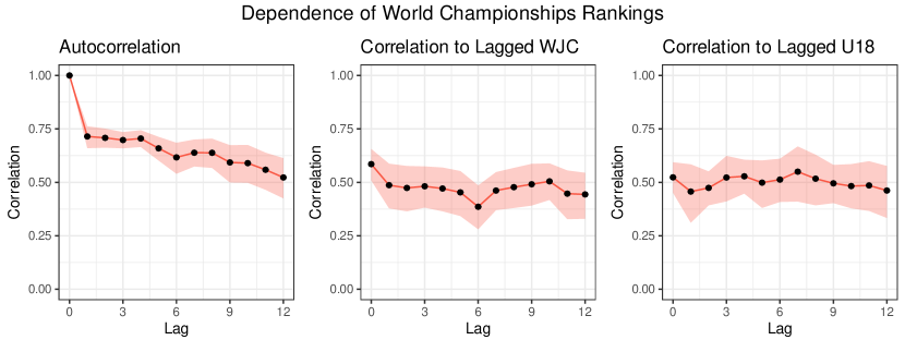
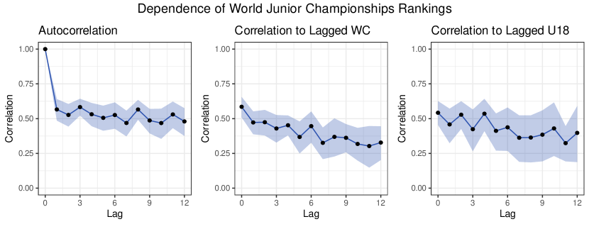
Figure 1: The autocorrelation of World Championships ranks, the correlation of World Championships ranks with lagged World Junior Championships ranks, and the correlation of World Championships ranks with lagged World Under-18 Championships ranks. The plots include 95 percent confidence bands obtained using the bootstrapping method.

Figure 2: The autocorrelation of World Junior Championships ranks, the correlation of World Junior Championships ranks with lagged World Championships ranks, and the correlation of World Junior Championships ranks with lagged World Under-18 Championships ranks. The plots include 95 percent confidence bands obtained using the bootstrapping method.

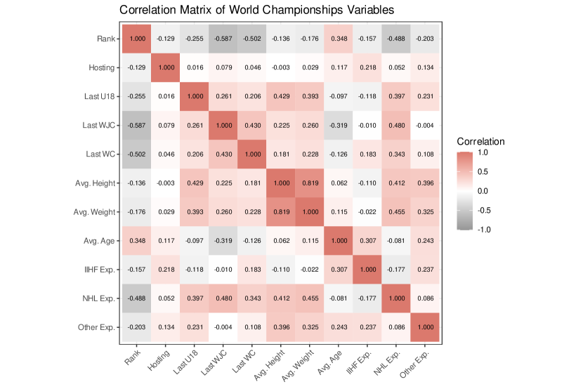
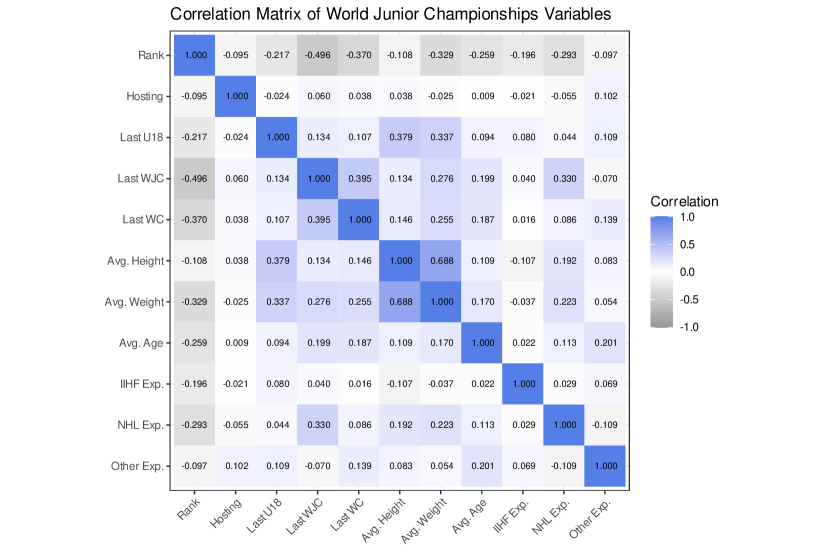
Figure 3: The correlations between the rank and the predictor variables for the World Championships.

Figure 4: The correlations between the rank and the predictor variables for the World Junior Championships.

Figures 4 and 4 illustrate the correlations between the World Championships and World Junior Championships rankings and predictor variables, revealing several intriguing patterns. There is a modest negative correlation between ranking and hosting the tournament, with values of -0.129 for the WC and -0.095 for the WJC, suggesting a potential home advantage. In the WC, hosting is also positively correlated with IIHF experience (the WC and Olympic tournaments). Past success in the WC, WJC, and U18 tournaments is positively correlated with present success in both the WC and WJC (note that variables Last U18, Last WJC, and Last WC are in the form of reciprocal ranks). Successful teams tend to have higher average height and weight in both the WC and WJC. Height and weight are positively correlated with NHL experience but not with IIHF experience in both tournaments. They are also strongly correlated with each other. In the WC, successful teams tend to be younger on average, whereas in the WJC, where the age limit is 20, successful teams tend to be older on average, i.e, closer to that upper age limit. Age is positively correlated with IIHF experience but not with NHL experience in the WC. Player experience in any of the studied tournaments is positively correlated with team success. Notably, NHL experience has a much stronger correlation with rank compared to IIHF experience, with values of -0.488 versus -0.157 in the WC, and -0.293 versus -0.196 in the WJC. Finally, there is a small negative correlation of -0.177 between IIHF and NHL experience in the WC. Of course, the implications of this correlation analysis are quite limited, and the joint effect of all predictor variables should be further studied, as we do in the following section.

4.2 Estimated Models

We turn to our proposed dynamic ranking model. We estimate seven models with various sets of predictor variables: the ‘static’ model utilizes constant strength parameters; the ‘dynamic’ model includes a dynamic component in the strength parameters but no predictor variables; the ‘tournament’ model features the hosting variable and variables capturing the most recent results from the WC, WJC, and U18 tournaments; the ‘physical’ model includes height, weight, and age variables along with the hosting variable; the ‘experience’ model incorporates the three variables capturing player experience and the hosting variable; the ‘full’ model includes all 10 predictor variables; and the ‘final’ model utilizes the set of variables that leads to the lowest Akaike information criterion. For estimation, we use the maximum likelihood method with bounds $\varphi\in[0,1)$ and $\alpha\geq 0$. We further discuss this issue and estimate unbounded models in Section 4.4.

First, we focus on analyzing the World Championships. The main results are reported in Table 3, and the time-varying strength parameters are illustrated in Figure 5. Based on the log-likelihood and Akaike information criterion, adding the dynamic component to the static model significantly improves the fit. The ‘dynamic’ model is mean-reverting, with a value of 0.736 for the autoregressive coefficient, indicating medium persistence. In models with predictor variables, the hosting variable is positive, suggesting a slight increase in the strength of the hosting team, but it is statistically insignificant except for the ‘physical’ model. Therefore, there is not enough evidence to support a distinct home advantage. Among the results from past tournaments, the reciprocal rankings from the most recent WJC and WC have a significantly positive effect, while the most recent U18 ranking is insignificant. Adding these tournament variables reduces the value of the score coefficient, as they introduce similar information to the model. Regarding the physical attributes of players, the findings suggest that, on average, it is better to have shorter, heavier, and younger players. However, the effects of height and weight are not statistically significant in the ‘full’ model. Age becomes statistically significant only when the experience variables are included, implying that younger players are preferable, provided they have the necessary experience. Among the experience variables, experience from IIHF tournaments is found to be much more important than NHL experience based on p-values, while experience from other national leagues is insignificant. The estimated coefficients for the experience variables should be interpreted in the context of the number of games played in IIHF tournaments versus the NHL, as reported in Table 1. In a single NHL season, teams play, on average, 11 times more games than in a single WC tournament. However, the estimated coefficient for IIHF experience is 25 times larger than that for NHL experience, indicating that participation in a single WC tournament is much more valuable than participation in a single NHL season. Adding the experience variables reduces the value of the autoregressive coefficient, as they account for a portion of the observed autocorrelation. Despite this, we retain the dynamic component in the model. The experience variables improve the fit the most compared to the tournament and physical variables. The final model that minimizes the Akaike information criterion, and has all predictor variables significant at the 0.1 level, includes the reciprocal rank from the last WJC and WC tournaments, the average age, and the average IIHF and NHL experience.

Next, we focus on analyzing the World Junior Championships. The main results are reported in Table 4, and the time-varying strength parameters are illustrated in Figure 6. Similar to the WC analysis, adding the dynamic component to the static model significantly improves the fit. The hosting variable is consistently significant across all models, indicating a clear home advantage for the hosting team. This suggests that younger players participating in the WJC are more negatively affected by playing in a foreign environment compared to the more seasoned players in the WC. The results from the most recent WC, WJC, and U18 tournaments are all found to be insignificant. The lack of dependence on the most recent WC is expected, as the overlap of players between the last WC and the current WJC is minimal. A similar situation occurs with the last WJC and the current WJC, as rosters often change dramatically from year to year. Some dependence on the last U18 tournament might be anticipated, given that many players transition from U18 to WJC, but it is ultimately found to be insignificant, even though the associated coefficient is the highest among the three tournaments. The average height and weight of players are significant, with the same signs as in the WC analysis: height has a negative impact, while weight has a positive impact. Age, however, is found to be insignificant, likely due to the small variation in the average age level within the WJC. Among the experience variables, only experience from IIHF tournaments is found to be relevant, while experience from the NHL and other leagues is insignificant. As in the WC analysis, including experience improves the model fit the most. The final model is obtained by minimizing the Akaike information criterion, and, as in the WC analysis, all predictor variables are significant at the 0.1 level. The variables included in the final model are the hosting variable, average height, average weight, and average IIHF experience.

Table 3: The estimated coefficients with the standard errors in parentheses, along with the fitted log-likelihood and the Akaike information criterion for various models of the World Championships. The models are estimated by the maximum likelihood method. The fixed effects for individual teams are omitted. The best attained values of the log-likelihood and the Akaike information criterion are highlighted.

	Static	Dynamic	Tourn.	Phys.	Exp.	Full	Final
Hosting			0.308	0.315∗	0.088	0.040
			(0.194)	(0.191)	(0.208)	(0.213)
Last U18			-0.001			0.036
			(0.334)			(0.343)
Last WJC			0.958∗∗∗			0.860∗∗∗	0.853∗∗∗
			(0.288)			(0.301)	(0.295)
Last WC			0.853∗∗∗			0.699∗∗	0.674∗∗
			(0.308)			(0.315)	(0.313)
Avg. Height				-0.107		-0.092
				(0.075)		(0.075)
Avg. Weight				0.136∗∗		0.071
				(0.058)		(0.058)
Avg. Age				-0.070		-0.222∗∗∗	-0.191∗∗∗
				(0.055)		(0.070)	(0.065)
IIHF Exp.					0.045∗∗∗	0.052∗∗∗	0.053∗∗∗
					(0.010)	(0.011)	(0.011)
NHL Exp.					-0.000	0.002	0.002∗
					(0.001)	(0.001)	(0.001)
Other Exp.					-0.001	0.001
					(0.001)	(0.001)
Autoreg. Coef.		0.736∗∗∗	0.747∗∗∗	0.756∗∗∗	0.591∗∗	0.677∗∗	0.674∗∗
		(0.114)	(0.146)	(0.103)	(0.292)	(0.323)	(0.321)
Score Coef.		0.186∗∗∗	0.078	0.190∗∗∗	0.136∗∗	0.039	0.040
		(0.060)	(0.063)	(0.061)	(0.069)	(0.070)	(0.068)
Log-Lik.	-765.832	-759.578	-749.232	-754.690	-747.819	-734.524	-735.989
AIC	1577.664	1569.155	1556.464	1567.380	1553.638	1539.047	1531.978
${}^{***}p<0.01$; ${}^{**}p<0.05$; ${}^{*}p<0.1$

Table 4: The estimated coefficients with the standard errors in parentheses, along with the fitted log-likelihood and the Akaike information criterion for various models of the World Junior Championships. The models are estimated by the maximum likelihood method. The fixed effects for individual teams are omitted. The best attained values of the log-likelihood and the Akaike information criterion are highlighted.

	Static	Dynamic	Tourn.	Phys.	Exp.	Full	Final
Hosting			0.488∗∗	0.557∗∗	0.587∗∗	0.673∗∗∗	0.653∗∗∗
			(0.239)	(0.242)	(0.241)	(0.248)	(0.247)
Last U18			0.542			0.494
			(0.394)			(0.396)
Last WJC			-0.131			-0.245
			(0.336)			(0.344)
Last WC			0.115			0.225
			(0.265)			(0.273)
Avg. Height				-0.195∗∗		-0.123	-0.142∗
				(0.082)		(0.083)	(0.082)
Avg. Weight				0.142∗∗		0.105∗	0.123∗
				(0.063)		(0.064)	(0.063)
Avg. Age				0.293		0.478
				(0.359)		(0.371)
IIHF Exp.					0.880∗∗∗	0.866∗∗∗	0.897∗∗∗
					(0.183)	(0.185)	(0.180)
NHL Exp.					0.070	0.084
					(0.059)	(0.060)
Other Exp.					0.009	0.007
					(0.008)	(0.008)
Autoreg. Coef.		0.850∗∗∗	0.834∗∗∗	0.788∗∗∗	0.852∗∗∗	0.800∗∗∗	0.796∗∗∗
		(0.121)	(0.152)	(0.242)	(0.105)	(0.190)	(0.177)
Score Coef.		0.070	0.059	0.060	0.079	0.060	0.059
		(0.048)	(0.062)	(0.058)	(0.051)	(0.069)	(0.056)
Log-Lik.	-442.939	-441.594	-438.577	-435.964	-424.753	-420.814	-424.078
AIC	913.877	915.189	917.153	911.927	889.506	893.628	888.157
${}^{***}p<0.01$; ${}^{**}p<0.05$; ${}^{*}p<0.1$

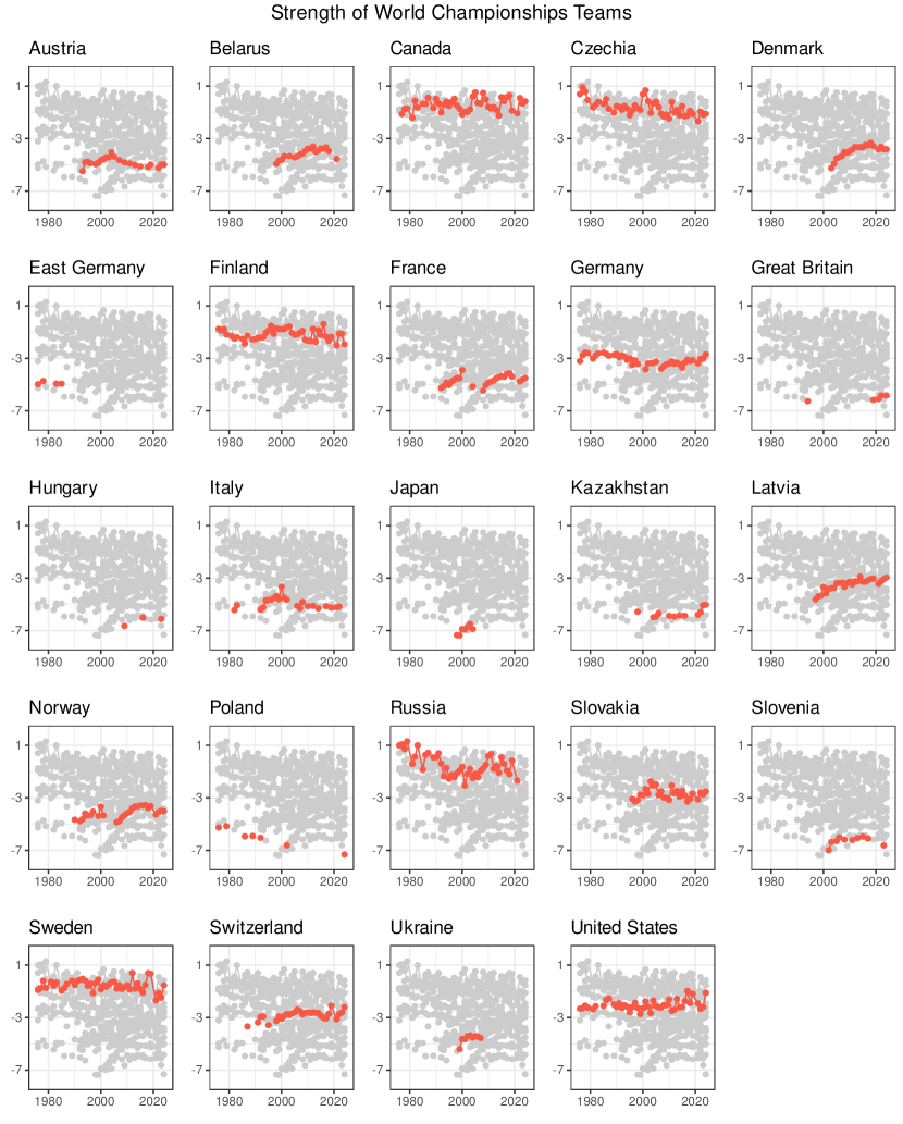
Figure 5: The time-varying strength parameters for individual teams in the World Championships. The strength parameters are obtained from the final model estimated by the maximum likelihood method. Only strength parameters for the years in which teams participated are included.

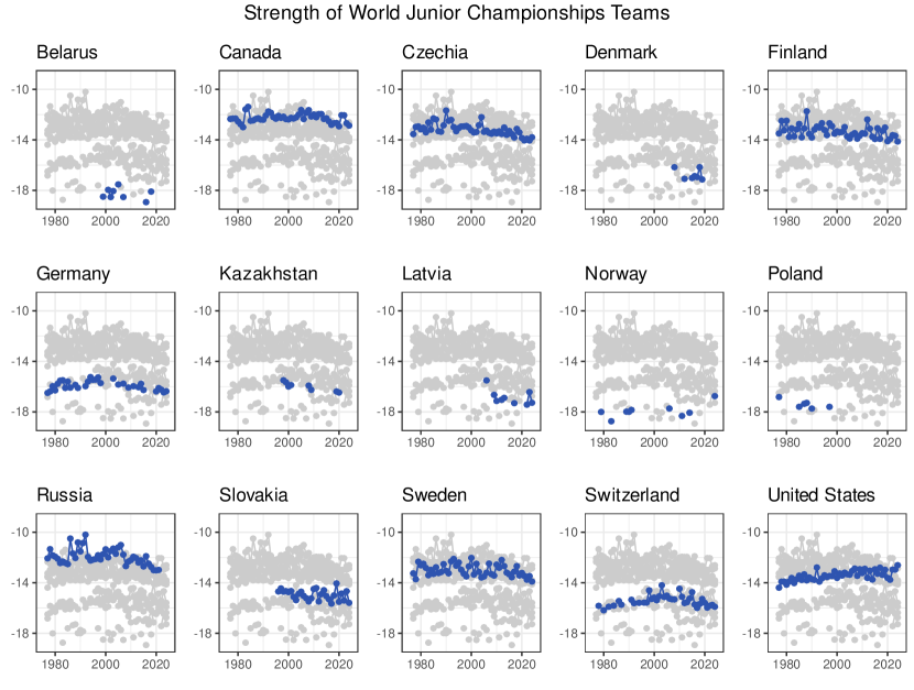
Figure 6: The time-varying strength parameters for individual teams in the World Junior Championships. The strength parameters are obtained from the final model estimated by the maximum likelihood method. Only strength parameters for the years in which teams participated are included.

4.3 Forecasting Performance

We evaluate the forecasting performance by re-estimating the models using the penalized maximum likelihood method with various values of the regularization parameter. We focus on the final specification of the predictor variables and compare it with the baseline static model. Rolling estimations with one-step-ahead forecasts are performed for the last 16 observations. We do not extend forecasts beyond the one-step-ahead horizon due to the unavailability of predictor variables for future tournaments. Even so, final rosters are announced just before the start of the tournaments, which affects the availability of the physical and experience variables. We compare the forecasts using several metrics, with the primary metric being the average log-likelihood of the one-step-ahead observation. To illustrate predictive ability, we assess three probabilities: the probability that the model correctly predicts the winner, the probability that the model correctly identifies the three medalists in any order, and the probability that the model correctly predicts which teams advance to the playoffs. Finally, we use the mean absolute error (MAE) and the root mean square error (RMSE) between the observed rankings and the modal rankings given by the model. We do not incorporate the mean ranking as it is computationally challenging to obtain. Therefore, the reported MAE and RMSE should be interpreted with caution.

The forecasting results are presented in Tables 5 and 6. When penalization is employed, the final model consistently achieves a higher log-likelihood than the static model. However, without penalization, the static model outperforms the final model. Note that in rolling estimation, the partition condition of Hunter (2004) does not always hold, making the use of penalization strongly advisable. Among the grid of values considered, the optimal regularization parameter $\lambda$ is found to be 0.01 for both WC and WJC, based on the average log-likelihood. The three probabilities studied reach their maximum values at lower $\lambda$ values; however, they remain relatively similar for $\lambda=0.01$. For WC, the final model with $\lambda=0.01$ correctly predicts the winner with a 17 percent probability, the three medalists with a 5 percent probability, and the eight teams advancing to the playoffs with a 3 percent probability. For WJC, the final model with $\lambda=0.01$ correctly predicts the winner with a 21 percent probability, the three medalists with a 7 percent probability, and the eight teams advancing to the playoffs with a 30 percent probability. Given that WC is played with 16 teams and WJC with 10 teams, the probabilities for advancing to the playoffs are naturally quite different. Regarding the evaluation of modal rankings, the lowest MAE and RMSE for WC are found with $\lambda=0.01$. For WJC, the lowest MAE is achieved with $\lambda=1$, while the lowest RMSE is achieved with $\lambda=0$, highlighting that the metrics based on the modal ranking may not be reliable. The MAE is 2.0 ranks for WC and 1.4 ranks for WJC when $\lambda=0.01$.

Table 5: The average predicted log-likelihood, the probabilities of winning the tournament, earning a medal, and advancing to the playoff phase, as well as the mean absolute error and the root mean squared error for one-step-ahead forecasts of the World Championships. The static and final models are estimated using the penalized maximum likelihood method with various values of the regularization parameter. The best attained values are highlighted.

	$\lambda=0$			$\lambda=0.001$			$\lambda=0.01$			$\lambda=0.1$			$\lambda=1$
Measure	Static	Final		Static	Final		Static	Final		Static	Final		Static	Final
Log-Lik.	-26.359	-29.270		-23.385	-23.413		-23.321	-22.783		-24.764	-23.669		-28.778	-27.793
P[Champion]	0.172	0.170		0.171	0.170		0.166	0.166		0.135	0.139		0.079	0.083
P[Medals]	0.032	0.050		0.032	0.050		0.028	0.045		0.015	0.022		0.003	0.004
P[Playoffs]	0.028	0.033		0.027	0.032		0.022	0.027		0.006	0.011		0.000	0.001
MAE	2.173	2.030		2.196	2.022		2.212	1.999		2.227	2.038		2.594	2.023
RMSE	2.766	2.657		2.787	2.651		2.812	2.627		2.844	2.668		3.314	2.647

Table 6: The average predicted log-likelihood, the probabilities of winning the tournament, earning a medal, and advancing to the playoff phase, as well as the mean absolute error and the root mean squared error for one-step-ahead forecasts of the World Junior Championships. The static and final models are estimated using the penalized maximum likelihood method with various values of the regularization parameter. The best attained values are highlighted.

	$\lambda=0$			$\lambda=0.001$			$\lambda=0.01$			$\lambda=0.1$			$\lambda=1$
Measure	Static	Final		Static	Final		Static	Final		Static	Final		Static	Final
Log-Lik.	-12.457	-13.380		-11.062	-10.949		-11.004	-10.794		-11.745	-11.072		-13.704	-13.080
P[Champion]	0.178	0.224		0.178	0.219		0.174	0.212		0.153	0.180		0.115	0.126
P[Medals]	0.058	0.073		0.058	0.075		0.054	0.071		0.036	0.049		0.014	0.017
P[Playoffs]	0.283	0.332		0.279	0.317		0.251	0.303		0.160	0.229		0.067	0.091
MAE	1.606	1.337		1.606	1.339		1.606	1.353		1.681	1.378		1.822	1.314
RMSE	2.081	1.763		2.081	1.795		2.081	1.805		2.145	1.837		2.391	1.796

4.4 Unbounded Optimization

For the in-sample analysis in Section 4.2 and the out-of-sample analysis in Section 4.3, we employed bounds $\varphi\in[0,1)$ and $\alpha\geq 0$. These bounds are quite natural, with $\varphi\geq 0$ and $\alpha\geq 0$ ensuring non-negative dependence on past strengths and tournament rankings, while $\varphi<1$ is necessary for stationarity. However, when estimation is performed without these bounds, the optimal value of $\varphi$ tends to approach 1, and $\alpha$ becomes negative, leading to results that lack a straightforward interpretation. Figures 8 and 8 illustrate this issue for the final models of both WC and WJC. These figures show the log-likelihood as a function of the score coefficient, with the remaining coefficients kept at their optimal values. We investigate the mean-reverting model with bounds $\varphi\in[0,1)$ and $\alpha\geq 0$, and the persistent model with $\varphi=1$ and unrestricted $\alpha$. However, for the mean-reverting model, only the bound $\alpha\geq 0$ would suffice, as the optimal $\varphi$ then lies in $\varphi\in[0,1)$. The persistent model resembles a random walk and is inherently non-stationary. In the positive region for both models, the log-likelihood functions appear to be concave. However, in the negative region, the functions exhibit irregular behavior, with several narrow peaks. In the case of unbounded estimation, one of these peaks becomes the global maximum. This irregular behavior poses significant challenges for numerical optimization algorithms, making it difficult to converge to this global maximum in the unbounded persistent model. Finding the global maximum may require multiple runs with different starting points. The persistent model with negative $\alpha$ is clearly overfitted, with even minor variations in $\alpha$, or any other coefficient, causing a significant drop in log-likelihood. Consequently, the estimated standard errors of all coefficients are close to zero, indicating an unreliable model. The forecasting performance of the persistent model with negative $\alpha$ is also notably poor. The average one-step-ahead log-likelihood is -25.723 for WC and -12.958 for WJC when $\lambda=0.01$, which is much worse than that of the proposed mean-reverting final model and even the static model. The cause of this strange behavior remains unclear, but is remarkably widespread: it appears in our models for both WC and WJC, with and without penalization, and is also observed in the model of Holý and Zouhar (2022) on a WC data sample with a reduced time frame. We recommend using bounds $\varphi\in[0,1)$ and $\alpha\geq 0$ to ensure an interpretable and well-behaved model.

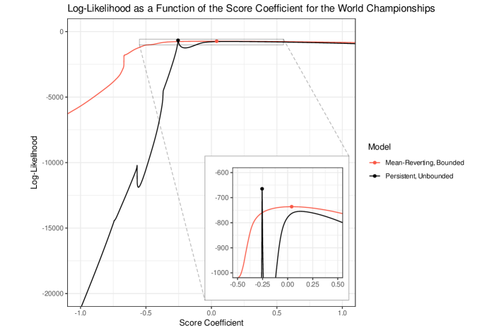
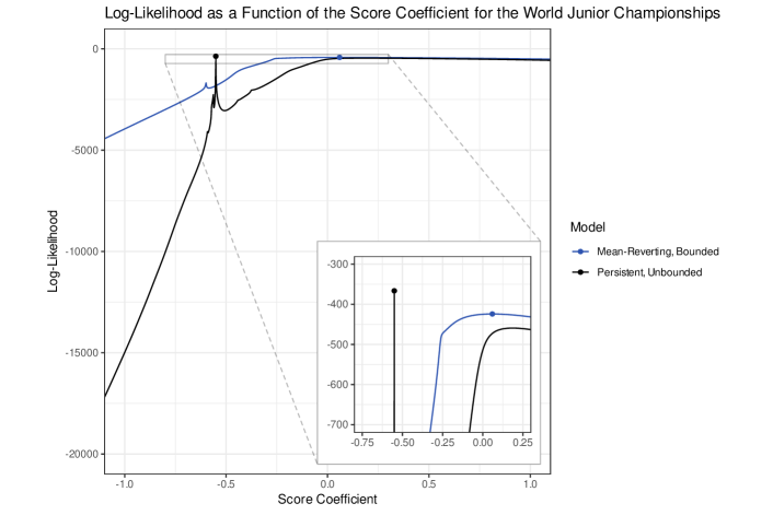
Figure 7: The value of the log-likelihood for varying values of the score coefficient in the World Championships. Other coefficients are kept at their optimal values. The mean-reverting final model, with bounds $\varphi\in(0,1)$ and $\alpha\geq 0$, and the persistent final model, with $\varphi=1$, are estimated using the maximum likelihood method.

Figure 8: The value of the log-likelihood for varying values of the score coefficient in the World Junior Championships. Other coefficients are kept at their optimal values. The mean-reverting final model, with bounds $\varphi\in(0,1)$ and $\alpha\geq 0$, and the persistent final model, with $\varphi=1$, are estimated using the maximum likelihood method and its penalized version.

5 Conclusion

We analyzed and forecasted the results of the World Championships and the World Junior Championships using a modified dynamic ranking model based on Holý and Zouhar (2022). Our analysis revealed notable differences in the factors influencing performance in the WC compared to the WJC. Home advantage was significant only for the WJC, suggesting that younger players are more affected by external environments. Success in the WJC positively influences subsequent performance in the WC, while success in the U18 was found to be insignificant for WJC performance. In terms of physical attributes, shorter and heavier players on average had a significant advantage in the WJC, while in the WC, these traits were less impactful. Younger teams in the WC tended to perform better, provided they had sufficient experience. A key finding is that experience in the past World Championships significantly outweighs experience in the NHL, challenging the commonly held belief in the superiority of the NHL. This suggests that the skill sets required for success in the WC and NHL differ. In forecasting, assuming stable strength levels over the long term and incorporating the above-described variables led to the most accurate predictions.

The methodology presented can be applied to any tournament and any team sport where final standings, i.e., complete rankings of all participating teams, are available. Future research could focus on challenging our assumption of the Plackett–Luce distribution and developing methods to include all teams in the sample without resorting to biased estimates through penalization. Both of these issues represent limitations of our study. Additionally, the behavior of the persistent model with a negative score coefficient warrants further investigation.

Funding

The work on this paper was supported by the Czech Science Foundation under project 23-06139S and the personal and professional development support program of the Faculty of Informatics and Statistics, Prague University of Economics and Business.

Appendix A Additional Tables and Figures

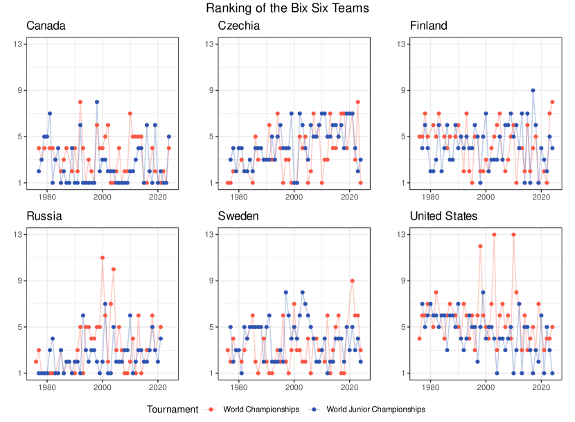
Figure 9: The rankings of the Big Six teams in the World Championships (43rd–87th editions) and the World Junior Championships (1st–48th editions). The source of data is IIHF (www.iihf.com).

Table 7: The total number of medals by country in the World Championships (1st–87th editions), World Junior Championships (1st–48th editions), and World Under-18 Championships (1st–25th editions). The source of data is IIHF (www.iihf.com).

	WC				WJC				U18
Team
Canada	28	16	9		20	10	5		5	1	4
Russia	27	10	10		13	13	11		3	6	3
Czechia	13	13	22		2	6	8			1	3
Sweden	11	19	18		2	12	7		2	6	6
Finland	4	9	3		5	5	7		4	3	5
United States	2	9	9		6	2	7		11	6	3
Great Britain	1	2	2
Slovakia	1	2	1				2			1	1
Switzerland		4	8				1			1
Germany		3	2
Austria			2
Latvia			1

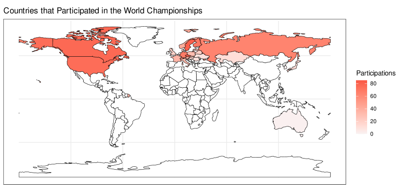
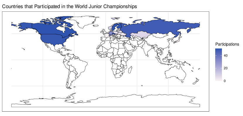
Figure 10: The total number of times participated in the World Championships (1st–87th editions). The national teams are visualized according to their most recent borders. The former teams of East Germany and Yugoslavia are omitted. The source of data is IIHF (www.iihf.com).

Figure 11: The total number of times participated in the World Junior Championships (1st–48th editions). The national teams are visualized according to their most recent borders. The source of data is IIHF (www.iihf.com).

Table 8: The five-number summary of the predictor variables for the World Championships.

Variable	Unit	Min	Q1	Q2	Q3	Max
Hosting	binary	0.00	0.00	0.00	0.00	1.00
Last U18	1 / rank	0.00	0.00	0.06	0.17	1.00
Last WJC	1 / rank	0.00	0.05	0.14	0.25	1.00
Last WC	1 / rank	0.00	0.08	0.12	0.25	1.00
Avg. Height	cm	175.00	182.10	183.52	184.79	189.42
Avg. Weight	kg	75.65	86.50	88.13	90.16	94.96
Avg. Age	years	22.88	25.63	26.60	27.61	31.24
IIHF Exp.	games	3.50	15.08	20.74	27.28	53.35
NHL Exp.	games	0.00	1.56	28.60	114.60	471.40
Other Exp.	games	0.00	30.73	89.05	208.83	438.24

Table 9: The five-number summary of the predictor variables for the World Junior Championships.

Variable	Unit	Min	Q1	Q2	Q3	Max
Hosting	binary	0.00	0.00	0.00	0.00	1.00
Last U18	1 / rank	0.00	0.00	0.00	0.20	1.00
Last WJC	1 / rank	0.00	0.14	0.20	0.33	1.00
Last WC	1 / rank	0.00	0.11	0.20	0.33	1.00
Avg. Height	cm	176.17	182.17	183.87	185.21	187.78
Avg. Weight	kg	78.92	85.25	87.52	89.82	96.18
Avg. Age	years	18.40	19.12	19.26	19.40	19.75
IIHF Exp.	games	0.00	0.00	0.00	0.40	2.10
NHL Exp.	games	0.00	0.00	0.00	0.22	12.00
Other Exp.	games	0.00	0.00	3.31	29.47	68.36

Table 10: The estimated fixed effects with the standard errors in parentheses for various models of the World Championships. The models are estimated by the maximum likelihood method.

	Static	Dynamic	Tourn.	Phys.	Exp.	Full	Final
Austria	-0.942∗∗∗	-0.933∗∗∗	-0.819∗∗∗	-1.007∗∗∗	-1.104∗∗∗	-0.776∗∗	-0.820∗∗∗
	(0.280)	(0.342)	(0.309)	(0.348)	(0.325)	(0.316)	(0.299)
Belarus	-0.164	-0.180	-0.078	-0.302	-0.341	-0.240	-0.179
	(0.283)	(0.366)	(0.320)	(0.383)	(0.332)	(0.323)	(0.309)
Canada	3.099∗∗∗	3.080∗∗∗	2.527∗∗∗	2.807∗∗∗	3.499∗∗∗	2.225∗∗∗	2.268∗∗∗
	(0.232)	(0.292)	(0.297)	(0.336)	(0.453)	(0.505)	(0.482)
Czechia	2.887∗∗∗	2.940∗∗∗	2.654∗∗∗	2.725∗∗∗	2.868∗∗∗	2.207∗∗∗	2.380∗∗∗
	(0.226)	(0.290)	(0.266)	(0.314)	(0.289)	(0.307)	(0.262)
Denmark	-0.073	-0.094	0.035	0.005	-0.368	-0.214	-0.334
	(0.258)	(0.358)	(0.303)	(0.372)	(0.321)	(0.306)	(0.295)
East Germany	-1.713	-1.751	-1.428	-1.555	-1.296	-1.144	-1.106
	(1.362)	(1.348)	(1.272)	(1.323)	(1.272)	(1.214)	(1.235)
Finland	2.425∗∗∗	2.368∗∗∗	2.138∗∗∗	2.249∗∗∗	2.303∗∗∗	1.605∗∗∗	1.852∗∗∗
	(0.229)	(0.286)	(0.262)	(0.295)	(0.344)	(0.364)	(0.254)
France	-0.744∗∗∗	-0.796∗∗	-0.607∗∗	-0.642∗	-1.116∗∗∗	-0.618∗∗	-0.756∗∗∗
	(0.258)	(0.321)	(0.289)	(0.333)	(0.311)	(0.311)	(0.293)
Germany	0.619∗∗∗	0.605∗∗	0.645∗∗∗	0.612∗∗	0.480∗	0.304	0.398∗
	(0.218)	(0.283)	(0.246)	(0.290)	(0.282)	(0.276)	(0.239)
Great Britain	-1.938∗∗∗	-2.005∗∗∗	-1.794∗∗∗	-1.830∗∗∗	-1.849∗∗∗	-0.828	-1.061
	(0.640)	(0.692)	(0.666)	(0.701)	(0.714)	(0.759)	(0.716)
Hungary	-2.150∗∗∗	-2.126∗∗∗	-1.966∗∗	-2.108∗∗	-1.759∗∗	-1.186	-1.384
	(0.808)	(0.820)	(0.815)	(0.829)	(0.830)	(0.881)	(0.860)
Italy	-0.996∗∗∗	-0.907∗∗∗	-0.792∗∗	-0.763∗∗	-1.148∗∗∗	-0.677∗	-0.764∗∗
	(0.291)	(0.350)	(0.320)	(0.373)	(0.342)	(0.353)	(0.321)
${}^{***}p<0.01$; ${}^{**}p<0.05$; ${}^{*}p<0.1$

Table 10 (Continued): The estimated fixed effects with the standard errors in parentheses for various models of the World Championships. The models are estimated by the maximum likelihood method.

	Static	Dynamic	Tourn.	Phys.	Exp.	Full	Final
Japan	-2.930∗∗∗	-2.811∗∗∗	-2.704∗∗∗	-2.166∗∗	-2.812∗∗∗	-2.221∗∗∗	-2.469∗∗∗
	(0.730)	(0.806)	(0.763)	(0.879)	(0.804)	(0.842)	(0.767)
Kazakhstan	-1.740∗∗∗	-1.761∗∗∗	-1.611∗∗∗	-1.583∗∗∗	-1.568∗∗∗	-1.000∗∗	-1.130∗∗
	(0.429)	(0.464)	(0.447)	(0.471)	(0.454)	(0.457)	(0.448)
Latvia	0.371	0.417	0.494∗	0.279	-0.005	0.057	0.128
	(0.236)	(0.329)	(0.279)	(0.346)	(0.307)	(0.292)	(0.282)
Norway	-0.227	-0.244	-0.104	-0.312	-0.588∗∗	-0.564∗	-0.553∗
	(0.241)	(0.310)	(0.274)	(0.321)	(0.298)	(0.288)	(0.283)
Poland	-2.465∗∗∗	-2.405∗∗∗	-2.329∗∗∗	-2.329∗∗∗	-2.169∗∗∗	-1.831∗∗	-1.838∗∗
	(0.766)	(0.773)	(0.778)	(0.778)	(0.779)	(0.795)	(0.778)
Russia	2.962∗∗∗	3.189∗∗∗	2.452∗∗∗	2.818∗∗∗	2.877∗∗∗	1.963∗∗∗	2.109∗∗∗
	(0.235)	(0.307)	(0.327)	(0.349)	(0.280)	(0.337)	(0.307)
Slovakia	0.994∗∗∗	1.011∗∗∗	0.999∗∗∗	0.899∗∗∗	0.996∗∗∗	0.861∗∗∗	0.880∗∗∗
	(0.243)	(0.329)	(0.280)	(0.347)	(0.290)	(0.280)	(0.261)
Slovenia	-2.317∗∗∗	-2.323∗∗∗	-2.158∗∗∗	-2.215∗∗∗	-2.240∗∗∗	-1.801∗∗∗	-1.948∗∗∗
	(0.500)	(0.541)	(0.521)	(0.548)	(0.523)	(0.523)	(0.509)
Sweden	3.032∗∗∗	2.971∗∗∗	2.633∗∗∗	2.983∗∗∗	3.209∗∗∗	2.515∗∗∗	2.622∗∗∗
	(0.229)	(0.288)	(0.275)	(0.304)	(0.314)	(0.348)	(0.276)
Switzerland	1.028∗∗∗	0.936∗∗∗	0.978∗∗∗	0.895∗∗∗	0.877∗∗	0.419	0.675∗∗
	(0.244)	(0.313)	(0.275)	(0.324)	(0.364)	(0.372)	(0.272)
Ukraine	-0.701∗	-0.786	-0.598	-0.838	-0.708	-0.257	-0.248
	(0.408)	(0.508)	(0.457)	(0.529)	(0.473)	(0.463)	(0.440)
United States	1.683∗∗∗	1.604∗∗∗	1.432∗∗∗	1.378∗∗∗	1.963∗∗∗	1.203∗∗∗	1.279∗∗∗
	(0.223)	(0.285)	(0.281)	(0.316)	(0.317)	(0.358)	(0.329)
${}^{***}p<0.01$; ${}^{**}p<0.05$; ${}^{*}p<0.1$

Table 11: The estimated fixed effects with the standard errors in parentheses for various models of the World Junior Championships. The models are estimated by the maximum likelihood method.

	Static	Dynamic	Tourn.	Phys.	Exp.	Full	Final
Belarus	-3.159∗∗∗	-3.133∗∗∗	-3.054∗∗∗	-2.932∗∗∗	-3.144∗∗∗	-2.994∗∗∗	-3.193∗∗∗
	(0.975)	(0.988)	(0.985)	(0.992)	(1.005)	(1.010)	(0.997)
Canada	2.706∗∗∗	2.663∗∗∗	2.704∗∗∗	2.593∗∗∗	2.806∗∗∗	2.625∗∗∗	2.797∗∗∗
	(0.249)	(0.285)	(0.317)	(0.314)	(0.345)	(0.398)	(0.318)
Czechia	1.741∗∗∗	1.808∗∗∗	1.745∗∗∗	1.635∗∗∗	1.867∗∗∗	1.694∗∗∗	1.791∗∗∗
	(0.230)	(0.271)	(0.271)	(0.278)	(0.291)	(0.301)	(0.283)
Denmark	-1.399∗∗	-1.395∗∗	-1.394∗∗	-1.313∗∗	-1.375∗∗	-1.185∗	-1.394∗∗
	(0.599)	(0.627)	(0.641)	(0.633)	(0.644)	(0.650)	(0.631)
Finland	1.656∗∗∗	1.644∗∗∗	1.532∗∗∗	1.518∗∗∗	1.307∗∗∗	1.226∗∗∗	1.530∗∗∗
	(0.231)	(0.267)	(0.273)	(0.260)	(0.372)	(0.366)	(0.261)
Germany	-0.771∗∗∗	-0.777∗∗∗	-0.763∗∗∗	-0.638∗∗	-0.804∗∗	-0.692∗∗	-0.651∗∗
	(0.274)	(0.300)	(0.295)	(0.296)	(0.312)	(0.309)	(0.301)
Kazakhstan	-0.981∗	-0.973∗	-0.858	-0.447	-0.751	-0.228	-0.381
	(0.549)	(0.569)	(0.574)	(0.643)	(0.582)	(0.652)	(0.645)
Latvia	-1.346∗∗∗	-1.338∗∗	-1.422∗∗	-1.331∗∗	-1.612∗∗∗	-1.419∗∗	-1.645∗∗∗
	(0.513)	(0.538)	(0.553)	(0.552)	(0.574)	(0.581)	(0.568)
Norway	-2.440∗∗∗	-2.443∗∗∗	-2.329∗∗∗	-2.333∗∗∗	-2.604∗∗∗	-2.541∗∗∗	-2.730∗∗∗
	(0.726)	(0.731)	(0.732)	(0.734)	(0.755)	(0.768)	(0.770)
Poland	-2.249∗∗	-2.298∗∗	-2.305∗∗	-2.529∗∗	-2.085∗∗	-2.323∗∗	-2.274∗∗
	(1.009)	(1.021)	(1.019)	(1.033)	(1.018)	(1.029)	(1.028)
Russia	2.847∗∗∗	2.856∗∗∗	2.811∗∗∗	2.578∗∗∗	2.998∗∗∗	2.714∗∗∗	2.720∗∗∗
	(0.252)	(0.288)	(0.320)	(0.315)	(0.299)	(0.361)	(0.319)
Slovakia	0.215	0.215	0.236	0.283	0.217	0.260	0.154
	(0.264)	(0.310)	(0.304)	(0.305)	(0.330)	(0.325)	(0.310)
Sweden	1.908∗∗∗	1.953∗∗∗	1.893∗∗∗	1.835∗∗∗	1.813∗∗∗	1.656∗∗∗	1.967∗∗∗
	(0.235)	(0.273)	(0.280)	(0.274)	(0.344)	(0.344)	(0.269)
Switzerland	-0.296	-0.356	-0.311	-0.395	-0.338	-0.307	-0.230
	(0.262)	(0.295)	(0.297)	(0.291)	(0.329)	(0.332)	(0.296)
United States	1.567∗∗∗	1.574∗∗∗	1.515∗∗∗	1.477∗∗∗	1.704∗∗∗	1.513∗∗∗	1.539∗∗∗
	(0.236)	(0.270)	(0.278)	(0.274)	(0.287)	(0.297)	(0.277)
${}^{***}p<0.01$; ${}^{**}p<0.05$; ${}^{*}p<0.1$

References

- Blasques et al. (2018) Blasques F, Gorgi P, Koopman SJ, Wintenberger O (2018). “Feasible Invertibility Conditions and Maximum Likelihood Estimation for Observation-Driven Models.” Electronic Journal of Statistics, 12(1), 1019–1052. ISSN 1935-7524. https://doi.org/10.1214/18-ejs1416.
- Blasques et al. (2014) Blasques F, Koopman SJ, Lucas A (2014). “Stationarity and Ergodicity of Univariate Generalized Autoregressive Score Processes.” Electronic Journal of Statistics, 8(1), 1088–1112. ISSN 1935-7524. https://doi.org/10.1214/14-ejs924.
- Blasques et al. (2022) Blasques F, van Brummelen J, Koopman SJ, Lucas A (2022). “Maximum Likelihood Estimation for Score-Driven Models.” Journal of Econometrics, 227(2), 325–346. ISSN 0304-4076. https://doi.org/10.1016/j.jeconom.2021.06.003.
- Buttrey et al. (2011) Buttrey SE, Washburn AR, Price WL (2011). “Estimating NHL Scoring Rates.” Journal of Quantitative Analysis in Sports, 7(3). ISSN 1559-0410. https://doi.org/10.2202/1559-0410.1334.
- Cox (1981) Cox DR (1981). “Statistical Analysis of Time Series: Some Recent Developments.” Scandinavian Journal of Statistics, 8(2), 93–108. ISSN 0303-6898. https://doi.org/10.2307/4615819.
- Creal et al. (2013) Creal D, Koopman SJ, Lucas A (2013). “Generalized Autoregressive Score Models with Applications.” Journal of Applied Econometrics, 28(5), 777–795. ISSN 0883-7252. https://doi.org/10.1002/jae.1279.
- Doyle and Leard (2012) Doyle JM, Leard B (2012). “Variations in Home Advantage: Evidence from the National Hockey League.” Journal of Quantitative Analysis in Sports, 8(2). ISSN 1559-0410. https://doi.org/10.1515/1559-0410.1446.
- Gorgi et al. (2019) Gorgi P, Koopman SJ, Lit R (2019). “The Analysis and Forecasting of Tennis Matches by Using a High Dimensional Dynamic Model.” Journal of the Royal Statistical Society: Series A (Statistics in Society), 182(4), 1393–1409. ISSN 0964-1998. https://doi.org/10.1111/rssa.12464.
- Groll et al. (2015) Groll A, Schauberger G, Tutz G (2015). “Prediction of Major International Soccer Tournaments Based on Team-Specific Regularized Poisson Regression: An Application to the FIFA World Cup 2014.” Journal of Quantitative Analysis in Sports, 11(2), 97–115. ISSN 1559-0410. https://doi.org/10.1515/jqas-2014-0051.
- Gu et al. (2019) Gu W, Foster K, Shang J, Wei L (2019). “A Game-Predicting Expert System Using Big Data and Machine Learning.” Expert Systems with Applications, 130, 293–305. ISSN 0957-4174. https://doi.org/10.1016/j.eswa.2019.04.025.
- Guérette et al. (2021) Guérette J, Blais C, Fiset D (2021). “The Absence of Fans Removes the Home Advantage Associated with Penalties Called by National Hockey League Referees.” PLoS ONE, 16(8 August), 1–15. ISSN 1932-6203. https://doi.org/10.1371/journal.pone.0256568.
- Harvey (2013) Harvey AC (2013). Dynamic Models for Volatility and Heavy Tails: With Applications to Financial and Economic Time Series. First Edition. Cambridge University Press, New York. ISBN 978-1-107-63002-4. https://doi.org/10.1017/cbo9781139540933.
- Holý (2024a) Holý V (2024a). “Package ’gasmodel’.” https://cran.r-project.org/package=gasmodel.
- Holý (2024b) Holý V (2024b). “Ranking-Based Second Stage in Data Envelopment Analysis: An Application to Research Efficiency in Higher Education.” Operations Research Perspectives, 12, 100306/1–100306/11. ISSN 2214-7160. https://doi.org/10.1016/j.orp.2024.100306.
- Holý and Zouhar (2022) Holý V, Zouhar J (2022). “Modelling Time-Varying Rankings with Autoregressive and Score-Driven Dynamics.” Journal of the Royal Statistical Society: Series C (Applied Statistics), 71(5), 1427–1450. ISSN 0035-9254. https://doi.org/10.1111/rssc.12584.
- Hunter (2004) Hunter DR (2004). “MM Algorithms for Generalized Bradley-Terry Models.” The Annals of Statistics, 32(1), 384–406. ISSN 0090-5364. https://doi.org/10.1214/aos/1079120141.
- Koopman and Lit (2019) Koopman SJ, Lit R (2019). “Forecasting Football Match Results in National League Competitions Using Score-Driven Time Series Models.” International Journal of Forecasting, 35(2), 797–809. ISSN 0169-2070. https://doi.org/10.1016/j.ijforecast.2018.10.011.
- Lasek and Gagolewski (2021) Lasek J, Gagolewski M (2021). “Interpretable Sports Team Rating Models Based on the Gradient Descent Algorithm.” International Journal of Forecasting, 37(3), 1061–1071. ISSN 0169-2070. https://doi.org/10.1016/j.ijforecast.2020.11.008.
- Leard and Doyle (2011) Leard B, Doyle JM (2011). “The Effect of Home Advantage, Momentum, and Fighting on Winning in the National Hockey League.” Journal of Sports Economics, 12(5), 538–560. ISSN 1527-0025. https://doi.org/10.1177/1527002510389869.
- Luce (1959) Luce RD (1959). Individual Choice Behavior: A Theoretical Analysis. First Edition. Wiley, New York. ISBN 978-0-486-44136-8. https://books.google.com/books/about/Individual{_}choice{_}behavior.html?id=a80DAQAAIAAJ.
- MacDonald (2011) MacDonald B (2011). “A Regression-Based Adjusted Plus-Minus Statistic for NHL Players.” Journal of Quantitative Analysis in Sports, 7(3). ISSN 1559-0410. https://doi.org/10.2202/1559-0410.1284.
- Marek et al. (2014) Marek P, Šedivá B, Ťoupal T (2014). “Modeling and Prediction of Ice Hockey Match Results.” Journal of Quantitative Analysis in Sports, 10(3), 357–365. ISSN 1559-0410. https://doi.org/10.1515/jqas-2013-0129.
- Plackett (1975) Plackett RL (1975). “The Analysis of Permutations.” Journal of the Royal Statistical Society: Series C (Applied Statistics), 24(2), 193–202. ISSN 0035-9254. https://doi.org/10.2307/2346567.
- Rowan (1990) Rowan TH (1990). Functional Stability Analysis of Numerical Algorithms. Doctoral thesis, The University of Texas at Austin. https://www.researchgate.net/publication/2487989.
- Schulte et al. (2017) Schulte O, Khademi M, Gholami S, Zhao Z, Javan M, Desaulniers P (2017). “A Markov Game Model for Valuing Actions, Locations, and Team Performance in Ice Hockey.” Data Mining and Knowledge Discovery, 31(6), 1735–1757. ISSN 1573-756X. https://doi.org/10.1007/s10618-017-0496-z.
- Tarter et al. (2009) Tarter B, Kirisci L, Tarter R, Jamnik V, Gledhill N, McGuire E (2009). “Use of the Sports Performance Index for Hockey (SPI-H) to Predict NHL Player Value.” International Journal of Performance Analysis in Sport, 9(2), 238–244. ISSN 2474-8668. https://doi.org/10.1080/24748668.2009.11868480.
- Thrane (2023) Thrane C (2023). “No Crowd, No Roar, No Home Advantage: Evidence from Ice Hockey.” European Sport Management Quarterly, 0(0), 1–13. ISSN 1746-031X. https://doi.org/10.1080/16184742.2023.2221684.
- Von Allmen et al. (2015) Von Allmen P, Leeds M, Malakorn J (2015). “Victims or Beneficiaries?: Wage Premia and National Origin in the National Hockey League.” Journal of Sport Management, 29(6), 633–641. ISSN 1543-270X. https://doi.org/10.1123/JSM.2014-0179.
- Whelan and Klein (2021) Whelan JT, Klein JE (2021). “Bradley-Terry Modeling with Multiple Game Outcomes with Applications to College Hockey.” Mathematics for Applications, 10(2), 157–177. ISSN 1805-3629. https://doi.org/10.13164/ma.2021.13.
- Ypma and Johnson (2020) Ypma J, Johnson SG (2020). “Package ’nloptr’.” https://cran.r-project.org/package=nloptr.
- Yu et al. (2019) Yu PLH, Gu J, Xu H (2019). “Analysis of Ranking Data.” Wiley Interdisciplinary Reviews: Computational Statistics, 11(6), e1483:1–e1483:26. ISSN 1939-5108. https://doi.org/10.1002/wics.1483.