Quantum Volunteer’s Dilemma
Abstract
The volunteer’s dilemma is a well-known game in game theory that models the conflict players face when deciding whether to volunteer for a collective benefit, knowing that volunteering incurs a personal cost. In this work, we introduce a quantum variant of the classical volunteer’s dilemma, generalizing it by allowing players to utilize quantum strategies. Employing the Eisert–Wilkens–Lewenstein quantization framework, we analyze a multiplayer quantum volunteer’s dilemma scenario with an arbitrary number of players, where the cost of volunteering is shared equally among the volunteers. We derive analytical expressions for the players’ expected payoffs and demonstrate the quantum game’s advantage over the classical game. In particular, we prove that the quantum volunteer’s dilemma possesses symmetric Nash equilibria with larger expected payoffs compared to the unique symmetric Nash equilibrium of the classical game, wherein players use mixed strategies. Furthermore, we show that the quantum Nash equilibria we identify are Pareto optimal. Our findings reveal distinct dynamics in volunteer’s dilemma scenarios when players adhere to quantum rules, underscoring a strategic advantage of decision-making in quantum settings.
Keywords: Volunteer’s dilemma Symmetric volunteer’s dilemma with cost sharing Quantum game theory Eisert–Wilkens–Lewenstein scheme Quantum strategies Nash equilibrium Pareto optimality
1 Introduction
The volunteer’s dilemma, first introduced by Diekmann in 1985 [1], is a famous -player game in game theory, wherein players must decide whether or not to volunteer and incur a personal cost for the benefit of the entire group. This dilemma encapsulates numerous real-world social traps [2] and explains various human behaviors [3, 4, 5, 6, 7], such as the bystander effect [8, 9, 10, 11, 12, 13], free-riding [14, 15, 16], diffusion of responsibility [17, 18, 19, 20], and the NIMBY (‘not in my backyard’) syndrome [21, 22]. The dilemma also extends beyond human interactions to non-human animal behaviors such as the transmission of predator information [3, 23, 24, 25, 26, 27, 28, 29, 30]. Animals that volunteer to transmit such information may inadvertently alert the predator and put themselves at risk to benefit the group, as seen in species like sooty mangabeys [25] and guppies [30]. This dilemma also occurs in cancer cells [31, 32, 33] and microbial populations [34, 35]. For instance, during toxin production in bacteria, each bacterium faces a decision: to either pay the metabolic cost of producing a toxin to reach the necessary threshold for successful invasion of the host, or rely on another bacterium to bear the cost [35].
Over the last few decades, extensive research has been conducted on the volunteer’s dilemma, with theoretical studies characterizing various properties of the game [36, 10, 37], and experimental investigations exploring the factors influencing volunteering choices and how closely actual behavior aligns with theoretical predictions [2, 38, 39, 40, 41, 14, 42, 43, 44, 45, 19, 46, 47, 48, 49]. Various versions of the dilemma have been studied, including Diekmann’s original symmetric volunteer’s dilemma [1], where volunteers all incur the same cost and players all receive the same benefit; the asymmetric volunteer’s dilemma [50, 51, 52, 46, 53], which allows volunteers to incur different costs and players to receive different benefits; the threshold volunteer’s dilemma [54, 55], which requires a threshold number of volunteers for producing the benefit; and the volunteer’s timing dilemma [51, 36], where players can observe each other’s actions and wait for someone else to volunteer, potentially leading to a state of mamihlapinatapai [56].
One significant volunteer’s dilemma variant, introduced by Weesie and Franzen in 1998 [57], involves cost-sharing among volunteers. In this variant, the cost incurred by the volunteers is divided amongst them, making it more applicable to many real-life scenarios [57, 58]. For example, when countries share a polluted water body, they all benefit if one country decides to bear the cleaning costs; however, the burden can be reduced if multiple countries share the expense [59, 60]. Another scenario involves saving a drowning child, where a group rescue is less risky than an individual effort [58].
In this study, we introduce a volunteer’s dilemma setting governed by the laws of quantum mechanics, where the outcomes of a quantum measurement performed on an entangled quantum system determine whether players volunteer, with each player having the ability to manipulate their local part of the system before the measurement. While there are various ways to realize such a quantum setting [61, 62], we choose the well-known quantization framework established in quantum game theory by Eisert, Wilkens, and Lewenstein in 1999 [63]. At the beginning of the game, players are provided with an entangled -qubit state, with each player holding one qubit. Players then independently decide which quantum operation from a designated set to perform on their respective systems. After players manipulate these systems, a collective measurement of the joint quantum state is performed, revealing whether each player volunteers or not.
For the payoff structure, we use the cost-sharing variant of the volunteer’s dilemma à la Weesie and Franzen [57]: if nobody volunteers, all players receive a payoff of 0; if players volunteer, each non-volunteer receives a payoff of and each volunteer receives a payoff of . In other words, 2 units are awarded if at least one player volunteers, and the overall cost of volunteering, which is 1 unit, is shared among all the volunteers. The expected payoff of each player is then given by the sum of each possible payoff value, multiplied by its corresponding probability, where the probability is determined by Born’s rule [64], which calculates the probability of each measurement outcome based on the pre-measurement joint quantum state of the system.
We assume that the players in our quantum volunteer’s dilemma are rational and self-interested [65]. Players’ decisions are the result of maximizing their own selfish payoff functions, conditional on their beliefs about the other players’ optimal behaviors. This could lead to decisions that result in Nash equilibria, from which no player can increase their own payoff unilaterally [66]. The main results of our work are threefold: first, we derive analytical expressions for the players’ expected payoffs, showing that they can be written in terms of sums of products of trigonometric functions. Second, using these analytical results, we prove that our quantum game reveals symmetric Nash equilibria with higher expected payoffs compared to the unique symmetric Nash equilibrium [57] found in the classical game, where players employ mixed strategies. Third, we establish that these symmetric Nash equilibria are Pareto optimal, meaning that no player can improve their payoff without reducing the payoff of another player [67]. These features of our quantum game make it both attractive and intriguing, offering insights into how quantum strategies can fundamentally alter the dynamics and outcomes of social dilemmas.
The rest of our paper is structured as follows. In Section 1.1, we survey some related work in classical and quantum game theory, emphasizing their significant progress in recent decades and their relevance to our study. In Section 2, we introduce various game-theoretic concepts that are applicable to both classical and quantum game theory. We then review some results in the classical volunteer’s dilemma, both with pure and mixed strategies. In Section 3, we define our quantum volunteer’s dilemma game and derive explicit expressions for the payoff functions of the players. We then analyze various quantum strategies and prove that some of these strategies are both Nash equilibria and Pareto optimal. Additionally, we prove that the payoffs achieved at these quantum Nash equilibria surpass those attainable in the corresponding classical game with mixed strategies, showcasing the quantum advantage in this context. Finally, in Section 4, we conclude with a summary of our results and an outlook on future research directions.
1.1 Related work
Game theory serves as a foundational framework across various disciplines, including economics, political science, and social science [66, 68]. It explores strategic interactions amongst multiple players, where the payoffs depend not only on each player’s decisions but also on the decisions made by others. Its modern origin can be traced back to von Neumann’s seminal work in 1928 [69], which established fundamental principles for analyzing decision-making in both cooperative and competitive situations. Two important solution concepts developed in game theory that are central to this study are the Nash equilibrium [70], where no player can increase their payoff by unilaterally changing their actions, and Pareto optimality [67], where it is impossible to make any player better off without simultaneously making another player worse off.
The advent of ideas in quantum computation in the 1990s sparked a new question: what if players had access to quantum strategies? This question was first explored by Meyer [71] and Eisert, Wilkens, and Lewenstein (EWL) [63] in 1999, leading to the development of quantum game theory. One notable quantum game is the quantum prisoner’s dilemma, which ceases to pose a dilemma if quantum strategies are allowed. Unlike the classical prisoner’s dilemma game, where players get trapped in non-Pareto optimal Nash equilibria, quantum strategies enable players to achieve Pareto optimal Nash equilibria [63, 72, 73, 74].
Since the pioneering works of Meyer and EWL, quantum game theory has expanded significantly, introducing a variety of new quantum games. These include quantum Parrondo’s games [75, 76], quantum market games [77], quantum cooperative games [78], the quantum battle-of-the-sexes game [79, 80, 81, 82, 83], the quantum minority game [84, 85], and the quantum chicken game (also known as the quantum hawk-dove game) [72, 83]. In many of these games, quantum strategies offer strategic advantages over classical ones. For example, the quantum battle-of-the-sexes game resolves the dilemma of multiple equilibria found in the classical version, leading to a unique solution [81]. Similarly, in the quantum chicken game, players using quantum strategies achieve a unique Nash equilibrium with a higher expected payoff compared to what they would achieve using symmetric classical mixed strategies [72]. Our work extends this body of research, demonstrating that a quantum advantage also emerges in the volunteer’s dilemma, which can be viewed as an -player generalization of the chicken game.
The original EWL framework has been extended to various settings, such as iterated [86, 48, 87], infinitely repeated [88, 89], multiplayer [84], multi-choice [90], continuous-variable [91], and Bayesian agent-based [92] scenarios. In these contexts, the quantum advantage often persists, sometimes giving rise to novel behavior. For example, in the multiplayer setting, it has been shown that such games can possess new forms of quantum equilibrium, where entanglement shared among multiple players enables novel cooperative behavior [84].
But what accounts for the advantage observed in quantum games? Various studies have explored the role of quantum resources, such as entanglement [93, 94, 95, 96, 97] and quantum discord [98, 99], in creating this advantage. Additionally, the impact of noise in quantum games has been extensively studied [100, 101, 102, 103, 104, 105, 106, 107, 108], revealing that in the presence of noise, a system may lose its quantum characteristics, reverting to classical behavior and thereby diminishing the quantum advantage. More recently, studies have focused on identifying conditions that specify appropriate unitary strategies within the EWL framework, further refining our understanding of quantum strategic interactions [109, 110, 111, 112, 113].
With the advent of small- and intermediate-scale quantum devices [114], various groups have experimentally demonstrated quantum games using platforms such as linear optics [115, 116], nuclear magnetic resonance [117, 118], ion traps [119], and superconducting devices, including IBM’s quantum computers accessible through the cloud [120]. These implementations serve as important benchmarks for early quantum devices and confirm that they operate as expected. Additionally, an interesting study by Chen and Hogg explored how well humans play quantum games [121]. Surprisingly, they found that even without formal training in quantum mechanics, participants nearly achieved the payoffs predicted by quantum game theory.
Quantum game theory has found diverse applications across a range of fields, including high-frequency trading [122], negotiations [123], reducing food waste in supply chains [124], sustainable development [125, 126, 127], cooperation between pharmaceutical companies [128], and open-access publishing [129]. A significant area of application is wireless communication, where quantum strategies can optimize spectrum-sharing in cognitive radio networks [130]. In traffic flow management, quantum game theory has been used to design optimal routing strategies, helping to reduce congestion and improve efficiency [131]. Furthermore, in the domain of quantum networks, quantum game-theoretic approaches have been employed to enhance entanglement distribution protocols, maximizing fidelity and minimizing latency in quantum communication [132]. Our work on the quantum volunteer’s dilemma contributes to this growing body of work by offering a framework that can help resolve social dilemmas or improve network coordination.
2 Preliminaries
2.1 Game-theoretic concepts
We begin by laying the groundwork for the concepts central to this paper. At the heart of game theory lies the notion of a game, which involves multiple players making strategic decisions. Each player is presented with a set of possible strategies, and their payoff is determined by their payoff function, evaluated based on the combination of strategies chosen by all players. We express this formally as follows.
Definition 1 (-player game).
For , an -player game (in strategic form) is a -tuple
| (1) |
where each is a set and each is a real-valued function.
In this context, represents the set of strategies available to player , and denotes the payoff function for player . The value indicates the payoff received by player when for each , the -th player chooses strategy . The -tuple is called a strategy profile, representing a complete specification of the strategies chosen by all players.
Next, we turn our attention to three key solution concepts in game theory. For the following definitions, we consider a strategy profile in the context of an -player game .
Definition 2 (Nash Equilibrium).
The strategy profile is a Nash equilibrium of if, for every player and for every alternative strategy , the following condition holds:
| (2) |
In other words, a Nash equilibrium is a strategy profile where no player can improve their payoff by unilaterally deviating from their current strategy, given that the strategies of all the other players remain unchanged [70].
In the special case where each player has only two possible strategies, 0 and 1, i.e., , a strategy profile is a Nash equilibrium if and only if for all ,
| (3) |
where is the binary vector that is zero everywhere except on the -th bit, where it is 1, and denotes binary addition.
A special type of Nash equilibrium is the symmetric Nash equilibrium, where all players adopt the same strategy. Formally:
Definition 3 (Symmetric Nash equilibrium).
The strategy profile is a symmetric Nash equilibrium of if it is a Nash equilibrium and all players choose the same strategy, i.e., .
Finally, we introduce the concept of Pareto optimality.
Definition 4 (Pareto optimal).
The strategy profile is Pareto optimal in if for every player and for every strategy profile , the following condition holds:
| (4) |
In other words, a strategy profile is Pareto optimal if improving one player’s payoff necessarily results in a decrease in another player’s payoff [67].
To conclude, the above solution concepts are fundamental in game theory as they provide insights into strategic interactions. Ideally, we seek strategy profiles that are both a Nash equilibrium and Pareto optimal, as these concepts align with the ideas of efficiency and fairness in strategic interactions.
2.2 Classical volunteer’s dilemma with pure strategies
The game we consider in this study is the volunteer’s dilemma, specifically the cost-sharing version introduced by Weesie and Franzen [57]. In this version, with players, each player decides between volunteering and abstaining. The payoffs of the game are structured as follows: if no players volunteer, all players receive a payoff of 0. If players volunteer, each non-volunteer receives a payoff of , while each volunteer’s payoff is . In other words, if at least one player volunteers, the reward of units is distributed to all players, while the total cost of units incurred by volunteering is divided equally among the volunteers. For simplicity, for the rest of this study, we take and .
To denote the players’ strategies numerically, we use 1 to represent volunteering and 0 to represent abstaining. With this notation, the above game, when players are restricted to pure classical strategies, is represented by the -tuple , where denotes the set of strategies available to player , and are the payoff functions. These functions, which correspond to [57, Eq. (1)] when and , are given by:
| (5) |
Here, , the Hamming weight of , denotes the number of players choosing to volunteer. The indicator function, represented by the Iverson bracket , equals 1 if (i.e., if at least one player volunteers) and 0 otherwise. The payoffs of the volunteer’s dilemma are summarized in table form in Table 1.
| Number of other players who volunteer | |||||||||||
| Strategy of player | 0 | 1 | 2 | ||||||||
|
|
|
|
||||||||
|
0 | 2 | 2 | 2 | 2 | ||||||
There are exactly Nash equilibria in the game , each characterized by exactly one player volunteering and every other player abstaining. In other words, the Nash equilibria, which are the strategy profiles that satisfy Eq. 3, are precisely those with Hamming weight . To prove that the strategy profile where exactly one player volunteers (i.e., ) is a Nash equilibrium, consider the case where player is the sole volunteer, i.e. and for all . If player chooses to switch to abstaining, then their payoff would drop to , as no other player would be volunteering. If another player chooses to volunteer alongside player , then that player’s payoff would decrease from to . Thus, no player can improve their payoff by unilaterally changing their decision, confirming that these strategy profiles are Nash equilibria. Conversely, the strategy profile where all players choose to abstain (i.e., ) cannot be a Nash equilibrium because any player could increase their payoff from 0 to a positive value by choosing to volunteer. Similarly, if more than one player volunteers (i.e, ), then any of the volunteers could increase their payoff from to by opting to abstain. Therefore, the strategy profiles where exactly one player volunteers are the only Nash equilibria in the game.
In the special case when the number of players , the volunteer’s dilemma simplifies to the well-known game of chicken, often depicted as follows: two drivers approach a narrow bridge from opposite directions. The first driver to turn aside allows the other to cross. If neither turns, they risk a potentially deadly head-on collision, which is the most disastrous outcome for both. Each driver prefers to avoid being labeled as the “chicken” by staying on course while hoping the other will swerve [140].
In this context, swerving corresponds to the strategy of volunteering, and heading straight (i.e., not swerving) corresponds to abstaining. The payoff structure in the volunteer’s dilemma can be mapped as follows: if both players volunteer (i.e., both swerve), they receive a payoff of 1. If one player volunteers (i.e., swerves) while the other abstains (i.e., heads straight), the volunteer receives a payoff of 1 while the abstainer receives a payoff of 2 (benefiting from avoiding a crash while not being called a chicken). If neither player volunteers (i.e., both head straight), they receive a payoff of 0 (equivalent to crashing).
The normal form representation of the chicken game, as a bimatrix, is illustrated in Table 2.
| (swerve) | (straight) | |
| (swerve) | ||
| (straight) |
Now, the above characterization of Nash equilibria specializes to the well-known result that, in the game of chicken, the Nash equilibria occur when one player swerves while the other goes straight. Notably, in both chicken and the more general -player volunteer’s dilemma, the Nash equilibria are not symmetric, meaning that players do not all adopt the same strategy. Given the symmetric nature of the payoffs, however, one might expect or prefer symmetric Nash equilibria. To achieve such equilibria, one approach is to modify the game to allow players to employ mixed strategies.
2.3 Classical volunteer’s dilemma with mixed strategies
Mixed strategies in the context of the volunteer’s dilemma involve players deciding to volunteer probabilistically rather than deterministically. Specifically, each player’s strategy set in this game is the unit interval , where a strategy of indicates that the player will choose to volunteer with probability . The payoff function for each player is the expected value of the payoff function from the deterministic game, with payoffs weighted by the probability of choosing to volunteer. This formulation interpolates between the pure strategies discussed in Section 2.2, with corresponding to volunteering (strategy ) and corresponding to abstaining (strategy ).
Formally, the classical volunteer’s dilemma with mixed strategies may be represented by the -tuple , where denotes the set of strategies available to player , and are the payoff functions, defined as
| (6) |
where are the payoff functions of the (deterministic) volunteer’s dilemma given by Eq. 5 and
| (7) |
denotes the joint probability that the strategy profile is chosen. The strategies of each player are assumed to be chosen independently and so the joint probability mass function factorizes; indeed, Eq. 7 can be written as , where is the probability that player volunteers, and is the probability that they abstain. We will refer to as the expected payoff of player under mixed strategies.
Unlike the volunteer’s dilemma with pure strategies , which has no symmetric Nash equilibria, the mixed-strategy game admits a unique symmetric Nash equilibrium. Interestingly, at this equilibrium, players volunteer with a probability that is a root of some univariate degree- polynomial whose coefficients depend on . More precisely, this result may be stated as follows:
Theorem 5 (Weesie and Franzen [57, Theorem 1i]).
The -player volunteer’s dilemma with mixed strategies has exactly one symmetric Nash equilibrium , where is the unique root in the open interval of the degree- polynomial given by
| (8) |
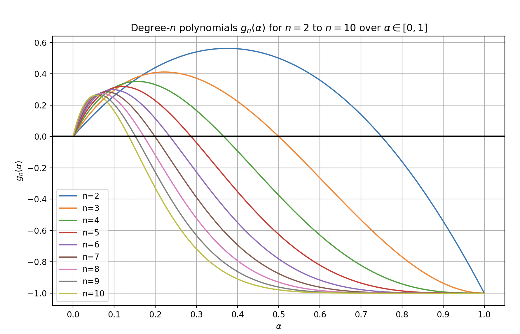
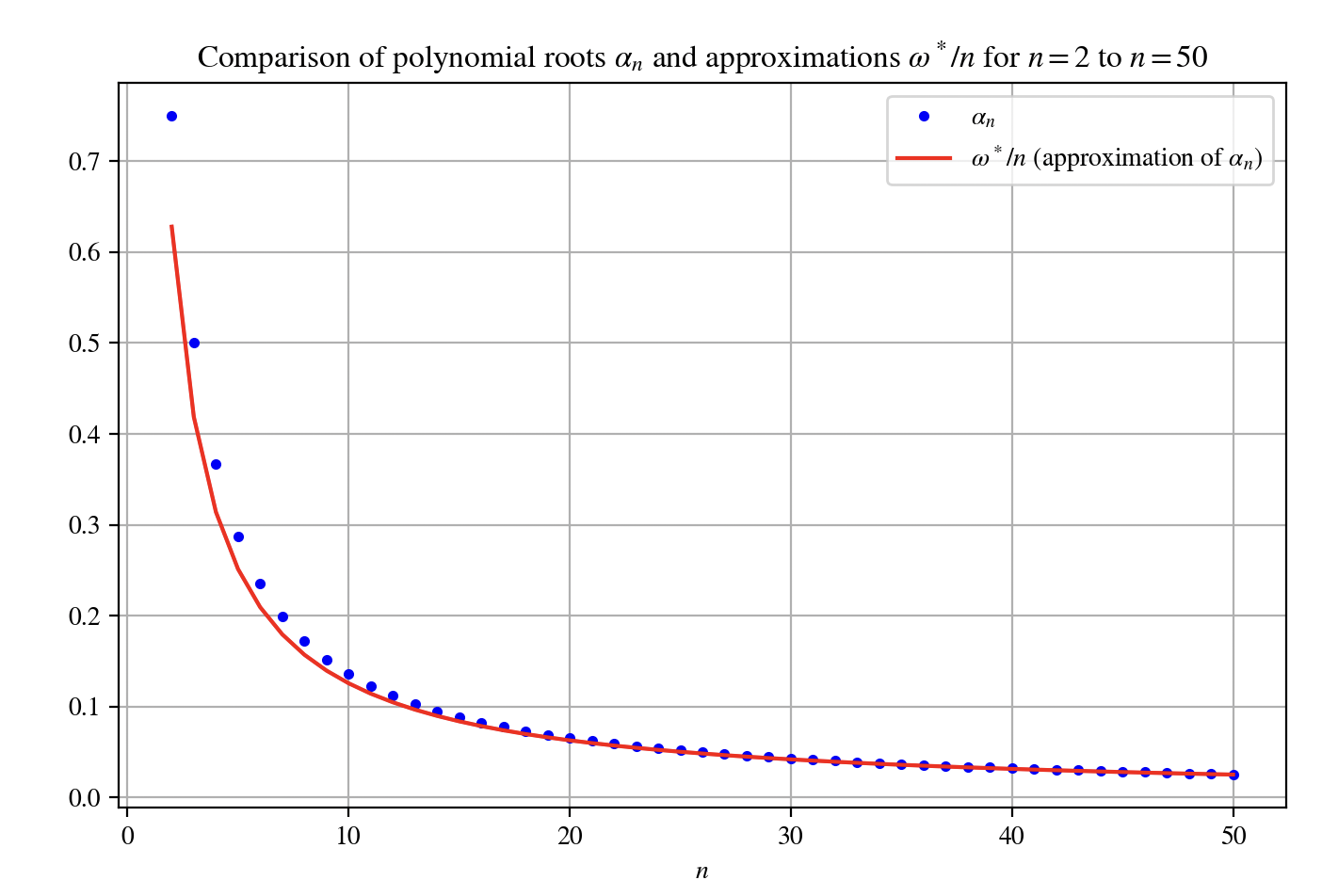
To illustrate the polynomials , we plot them over the interval for to in Figure 1. As can be seen from this plot, the unique root of in decreases as increases. For large , the root asymptotically behaves as [57, Theorem 1ii]:
| (9) |
where is the unique positive solution for of the equation
| (10) |
with denoting the -th branch of the Lambert W-function evaluated at , implemented in the Wolfram Language as ProductLog[k,z] [141, 142]. To illustrate the decreasing trend of and its behavior for large , we present a plot of versus and compare it with the approximation in Figure 2.
Our next theorem provides an expression for the expected payoff of each player when players choose the unique symmetric Nash equilibrium strategy profile.
Theorem 6.
For the -player classical volunteer’s dilemma with mixed strategies , when the unique symmetric Nash equilibrium strategy profile is chosen, the expected payoff of each player defined by Eq. 6 evaluates to
| (11) |
Proof.
Consider the scenario in which every player chooses to volunteer with probability , and let be the event where every player abstains. The probability of the event is given by
In this case, the conditional expected payoff for each player is
| (12) |
as there are no volunteers.
Next, consider the complement event , where at least one player volunteers. By the complement rule, the probability of this event is
If the number of volunteers is , then the total payoff distributed among all players is . Consequently, given that at least one player volunteers, the conditional expected payoff for each player is
| (13) |
Therefore, by the law of total expectation, the expected payoff for each player can be expressed as
which completes the proof of the theorem. ∎
A few remarks about the expected payoff given in Eq. 11 are in order. First, note that the expression since . Consequently, the expected payoff of each player is bounded above as follows:
| (14) |
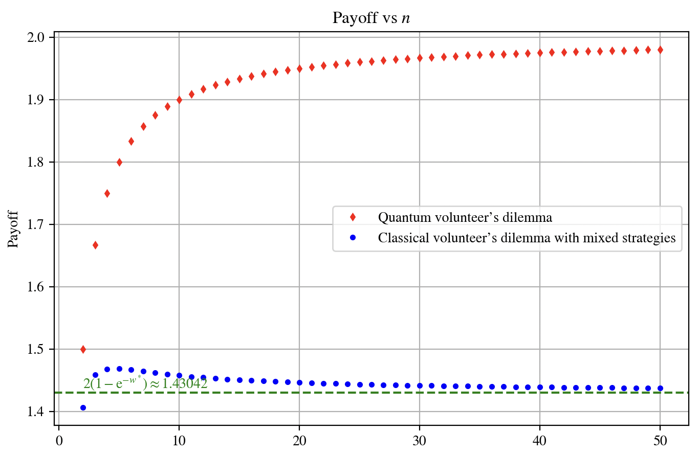
Second, for large , scales as , with this approximation being valid when neglecting terms of order and smaller (Eq. 9). Hence, in the limit as approaches infinity, the expected payoff converges to
| (15) |
The relational statements in Eqs. 14 and 2.3 can be contrasted with those for the quantum volunteer’s dilemma, which we will introduce in Section 3. In contrast to the strict upper bound in Eq. 14, where the classical payoff is strictly less than , the quantum volunteer’s dilemma can achieve symmetric Nash equilibria where the payoff of each player equals . Moreover, whereas the limit of the payoff in the classical game as approaches infinity is , the quantum game’s limit is significantly larger, approaching . This increase in payoffs underscores the advantage of the quantum game over its classical counterpart. We compare the payoffs at these symmetric Nash equilibria for both the classical and quantum games in Figure 3.
3 Quantum volunteer’s dilemma
We now introduce the quantum volunteer’s dilemma, which extends the classical volunteer’s dilemma by allowing players to use quantum strategies rather than classical ones, following the Eisert–Wilkens–Lewenstein quantization framework [63].
3.1 Game setup
The quantum volunteer’s dilemma game begins with players receiving an -qubit entangled state, with each player controlling one qubit. We fix the shared state as , where is the -qubit entangling unitary operator
| (16) |
where is the Pauli-Y matrix.
Each player independently selects a quantum operation from a designated set to apply to their respective qubit. We shall fix this set to be the two-parameter family of unitaries , where
| (17) |
Note that choosing a strategy from the above two-parameter strategies amounts to selecting two real parameters and . Accordingly, we represent each player’s strategy set by , and say that player ’s strategy is if they select the operation to perform on their qubit. Let denote the -fold Cartesian product of and denote its elements by .
After the players apply their quantum operation , a collective measurement is performed. We fix this measurement to be the -qubit entangling measurement conducted in the basis . Equivalently, this can be achieved by applying the entangling gate followed by a computational basis measurement. We associate the -th bit of the measurement outcome with whether player volunteers, with indicating that they volunteer, and indicating that they abstain. The quantum circuit depicted in Section 3.1 provides a visual summary of these steps.
| (18) | |||
| (19) | |||
| (20) | |||
| (22) | |||
| (24) | |||
Note that the quantum volunteer’s dilemma reduces to the classical volunteer’s dilemma with mixed strategies, as discussed in Section 2.3, if the players can choose only those in Eq. 17 where . In this case, volunteering is represented by , and abstaining represented by .
The probability distribution resulting from the measurement may be expressed as follows. If players choose the parameters and , the pre-measurement state before the computational basis measurement is performed is given by
| (25) |
For a string , let denote the string where each bit in is flipped, i.e., . Let and represent the amplitude and probability, respectively, of observing the binary string when the state is measured in the computational basis. According to Born’s rule, the amplitude and probability of measuring are
| (26) | ||||
| (27) |
Thus, is the probability that players in volunteer and players in abstain, where denotes the support of the string .
The expected payoff of player is then given by
| (28) |
where represents the payoff functions in the deterministic volunteer’s dilemma as defined in Eq. 5 and is defined in Eq. 27.
Formally, the -player quantum volunteer’s dilemma can be represented by the -tuple
| (29) |
where are the strategy sets and , defined by Eq. 28, are the payoff functions.
3.2 Analytical expressions for the payoff functions
The goal of this section is to simplify the expression for the payoff function in Eq. 28. To achieve this, we first introduce some auxiliary functions that will help us represent the payoff functions more compactly. Let
| (30) | ||||
| (31) |
The product of these functions is given by
| (32) |
where the last line follows from the double-angle identity .
We now present an analytical expression for the payoff functions.
Lemma 7.
Proof.
| (35) |
To prove Eq. 34, consider how the quantum state evolves through each step in the circuit shown in Section 3.1. The entangled state that the players receive is
| (36) |
After the players apply their local operations, the state becomes
| (37) |
On the other hand, the elements of the measurement basis can be written as
| (38) |
Substituting the expressions for the matrix elements , , , and into Eq. 39, we get
| (40) |
Squaring these amplitudes gives the probabilities:
| (41) |
The amplitude given by Eq. 40 can be either real or have a non-zero imaginary component, depending on whether is even or odd. Specifically, when is even, is real, whereas for odd , is imaginary. In light of this, when evaluating the probability , we will consider these two cases separately.
Case 1: is even. When is even, , and hence the amplitude given by Eq. 40 is real. Therefore, the probability expression simplifies to the square of this real amplitude.
| (42) |
where the last line follows from the fact that .
Case 2: is odd. When is odd, is purely imaginary. Therefore, the probability expression simplifies as follows:
| (43) |
3.3 Symmetric Nash equilibria for
In this section, we will exhibit the existence of a symmetric Nash equilibrium for the quantum volunteer’s dilemma with that yields a higher payoff compared to the classical volunteer’s dilemma with mixed strategies. As we will show in our next theorem, this symmetric Nash equilibrium occurs when all players choose the strategy , i.e., when the strategy profile is . This corresponds to each player applying the unitary operator
| (45) |
to their respective quantum systems.
Our next theorem also establishes that with the strategy profile , each player will volunteer with probability 1, meaning that the probability distribution in Eq. 44 becomes the degenerate distribution , resulting in each player’s payoff being . Here denotes the all-ones string.
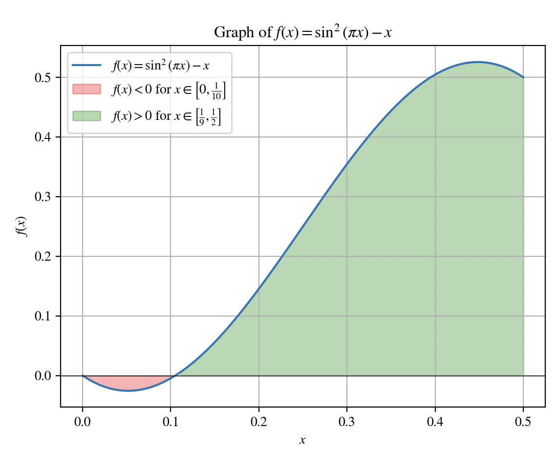
The key difference in Nash equilibrium behavior between and arises from the following lemma concerning the function . The behavior of is illustrated in Figure 5, which helps to visualize the regions where is positive or negative.
Lemma 8.
Let . Then,
| (46) |
Proof.
Let . We first evaluate the function at a few points of interest: , , , and .
Since is continuous, it is sufficient to show that has exactly one minimum point in the interval and exactly one maximum point in the interval . To establish this, we compute the first two derivatives of , solve for the stationary points, and determine whether these points are maxima or minima within the interval :
| (47) |
To find the stationary points, set
| (48) |
The intersection of the above set with the interval , which we are interested in, contains only two stationary points, namely
| (49) |
We check that and . Thus, is the unique local minimum in the interval and is the unique local maximum in the interval . This concludes the proof of the lemma. ∎
We now use Lemma 8 to prove our main theorem about the strategy profile .
Theorem 9.
For the -player quantum volunteer’s dilemma , if the players adopt the strategy profile , then every player volunteers with probability , i.e., the probability distribution is given by , and the corresponding payoff of each player is
| (50) |
Moreover,
-
a)
if , then is a Nash equilibrium of , and
-
b)
if , then is not a Nash equilibrium of .
Proof.
To calculate the probability that each player volunteers, we use the expression in Eq. 34 derived in Lemma 7. At the strategy profile , the functions defined in Eq. 30, Eq. 31, and Eq. 32 simplify as follows:
| (51) | ||||
| (52) | ||||
| (53) |
Hence, , i.e., . In other words, every player volunteers with probability . Substituting this expression into Eq. 33 yields the following payoff for each player :
| (54) |
But the set is empty unless , in which case it is equal to the singleton set . Hence,
| (55) |
where is the Kronecker delta.
Next, to determine whether is a Nash equilibrium, we examine the scenario where a specific player potentially deviates from , while all other players maintain the strategy . We begin by calculating the payoff for player under these conditions.
| (56) |
Similarly,
| (57) |
Since and have disjoint supports, it follows that their product vanishes. Hence, the probability of observing the outcome is
| (58) |
where the upward arrows indicate that the 0 or 1, respectively, is located at the -th position in the binary string.
Therefore, the payoff of player is
-
a)
Consider the case where . For any , we will show that the payoff of the -th player, when all other players adopt the strategy , is bounded above by . Indeed,
where the inequality on the last line follows from Lemma 8 with . Therefore, the strategy provides the optimal payoff for player when all other players also choose the strategy . Since the same reasoning applies to every player , the strategy profile is a Nash equilibrium.
-
b)
Consider the case where . For any player , we will demonstrate that if all other players adopt the strategy , there exists an alternative strategy for player that results in a higher payoff than if they were to choose , where the payoff from choosing would be . This shows that cannot be a Nash equilibrium.
Indeed, an example of an alternative strategy is the choice . With this strategy, the payoff for player evaluates to
(59) where the inequality on the last line follows from Lemma 8. Hence is not a Nash equilibrium for .
By combining the results above, we conclude that is a Nash equilibrium if and only if . ∎
3.4 Symmetric Nash equilibria for even
In this section, we shift our focus from the previously discussed symmetric Nash equilibria to a new family of symmetric Nash equilibria for cases with an even number of players. In this new strategy profile, each player adopts the strategy , resulting in a collective strategy profile . This choice corresponds to each player applying the unitary operator
| (60) |
to their respective quantum systems, where is the Pauli-Z matrix. Like , we will show that this new strategy profile yields a payoff of , surpassing the payoff of the symmetric Nash equilibrium in the classical volunteer’s dilemma.
Theorem 10.
In the -player quantum volunteer’s dilemma , if the players adopt the strategy profile , then every player volunteers with probability when is even, while every player abstains with probability when is odd, i.e.,
| (61) |
and the corresponding payoff of each player is
| (62) |
Moreover,
-
a)
if is even, then is a Nash equilibrium of , and
-
b)
if is odd, then is not a Nash equilibrium of .
Proof.
To calculate the probability that each player volunteers, we use the expression in Eq. 34 derived in Lemma 7. At the strategy profile , the functions defined in Eq. 30, Eq. 31, and Eq. 32 simplify as follows:
| (63) |
Similarly,
| (64) |
Since vanishes whenever is odd and vanishes whenever is even, their product must always vanish regardless of , i.e., . Consequently, the probability expression in Eq. 44 simplifies to
| (65) |
which gives the expression in Eq. 61. In other words, when the number of players is even, then every player would volunteer with probability , and when the number of players is odd, then every player would abstain with probability .
Next, to determine whether is a Nash equilibrium, we consider the scenario where a specific player potentially deviates from the strategy , while all other players continue to follow the strategy . Under these conditions, the payoff for player may be calculated as follows:
| (67) |
where the last line follows from the identity:
| (68) |
Similarly,
| (69) |
where the last line follows from the identity:
| (70) |
Since Eq. 67 and Eq. 69 are nonzero for disjoint sets of , their product . Hence, the corresponding probability evaluates to
| (71) |
We will now consider the cases where is even and is odd separately.
-
a)
When is even, the probability distribution simplifies to
(72) (73) Hence, the payoff for player evaluates to
(74) Therefore, the strategy provides the optimal payoff for player when all other players also choose the strategy . Since the same reasoning applies to every player , the strategy profile is a Nash equilibrium.
-
b)
When is odd, the probability distribution simplifies to
(75) Hence, the payoff for player evaluates to
(76) Now, suppose that player chooses the parameters and . Then Eq. 76 evaluates to
(77) which exceeds the payoff of that they would receive by following strategy . Hence, when is odd, is not a Nash equilibrium.
By combining the results above, we conclude that is a Nash equilibrium if and only if is even. ∎
3.5 Pareto optimality
In Sections 3.3 and 3.4, we presented two distinct families of symmetric Nash equilibria. In this section, we will demonstrate that these Nash equilibria are also Pareto optimal, as defined earlier in Definition 4. More broadly, we will prove that any strategy profile where every player receives a payoff of must be Pareto optimal. This includes the strategy profile , as well as the strategy profile when is even, both of which satisfy this payoff condition.
Theorem 11.
Let be any strategy profile for which for all . Then is Pareto optimal in the -player quantum volunteer’s dilemma .
Proof.
To prove that is Pareto optimal, it suffices to show that for any player and any strategy profile , if , then there exists another player such that .
To establish this, fix a player and a strategy profile such that , i.e.,
| (78) |
Suppose, for the sake of contradiction, that there does not exist any other player such that . By de Morgan’s laws for quantifiers, this assumption is equivalent to for all , i.e.,
| (79) |
Taking the sum of Eq. 78 and the sum over all of Eq. 79, we obtain
| (80) |
which implies that
| (81) |
Now, the first sum in Eq. 81 simplifies to
| (82) |
and the second sum in Eq. 81 simplifies to
| (83) |
Substituting Eqs. 82 and 83 back into Eq. 81 yields:
| (84) |
which is a contradiction, since cannot be less than itself.
Therefore, there must exist another player for which . This concludes the proof that is Pareto optimal. ∎
A straightforward corollary of Theorem 11 is that those strategy profiles and where each player’s payoff is are Pareto optimal. We state this formally as follows:
Corollary 12.
In the -player quantum volunteer’s dilemma , the following strategy profiles are Pareto optimal:
-
a)
, for all ,
-
b)
, for all even .
Proof.
4 Conclusion
In this study, we explored a quantum generalization of the classical volunteer’s dilemma by incorporating quantum strategies, utilizing the quantization framework introduced by Eisert, Wilkens, and Lewenstein [63]. Our analysis of the quantum volunteer’s dilemma with multiple players reveals key insights into the strategic advantages of decision-making in a quantum context.
We derived explicit analytical expressions for the expected payoffs of players, demonstrating that the quantum version of the game offers crucial advantages over its classical counterpart. Specifically, the quantum volunteer’s dilemma features symmetric Nash equilibria— for and for even —which yield higher expected payoffs compared to the unique symmetric Nash equilibrium of the classical game, where players employ mixed strategies. Notably, these Nash equilibria we identified are also Pareto optimal.
Our findings contribute to a deeper theoretical understanding of how quantum mechanics can impact strategic interactions in game theory. By highlighting the benefits of quantum strategies, this work paves the way for exploring their practical implementations and potential applications in diverse real-world contexts.
Acknowledgements
D.E.K. acknowledges funding support from the National Research Foundation, Singapore and the Agency for Science, Technology and Research (A*STAR) under its Quantum Engineering Programme (NRF2021-QEP2-02-P03), A*STAR C230917003, and A*STAR under the Central Research Fund (CRF) Award for Use-Inspired Basic Research (UIBR).
Competing interests
The authors declare no competing interests.
Data Availability
Data sharing is not applicable to this article as no datasets were generated or analyzed during the current study.
References
- [1] Andreas Diekmann. Volunteer’s dilemma. Journal of Conflict Resolution, 29(4):605–610, 1985. doi: 10.1177/0022002785029004003.
- [2] Andreas Diekmann. Volunteer’s Dilemma. A Social Trap without a Dominant Strategy and some Empirical Results, pages 187–197. Physica-Verlag HD, Heidelberg, 1986. doi: 10.1007/978-3-642-95874-8_13.
- [3] Marco Archetti. The volunteer’s dilemma and the optimal size of a social group. Journal of Theoretical Biology, 261(3):475–480, 2009. doi: 10.1016/j.jtbi.2009.08.018.
- [4] Marco Archetti. Cooperation as a volunteer’s dilemma and the strategy of conflict in public goods games. Journal of evolutionary biology, 22(11):2192–2200, 2009. doi: 10.1111/j.1420-9101.2009.01835.x.
- [5] Young-joo Lee and Jeffrey L. Brudney. Rational volunteering: a benefit-cost approach. International Journal of Sociology and Social Policy, 29(9/10):512–530, Jan 2009. doi: 10.1108/01443330910986298.
- [6] Joachim I. Krueger. The vexing volunteer’s dilemma. Current Directions in Psychological Science, 28(1):53–58, 2019. doi: 10.1177/0963721418807709.
- [7] Florian Heine, Arjen van Witteloostuijn, and Tse-Min Wang. Self-sacrifice for the Common Good under Risk and Competition: An Experimental Examination of the Impact of Public Service Motivation in a Volunteer’s Dilemma Game. Journal of Public Administration Research and Theory, 32(1):217–232, 07 2021. doi: 10.1093/jopart/muab017.
- [8] Bibb Latané and John M Darley. The unresponsive bystander: Why doesn’t he help? New York: Appleton Century-Crofts, 1970.
- [9] Karthik Panchanathan, Willem E Frankenhuis, and Joan B Silk. The bystander effect in an -person dictator game. Organizational Behavior and Human Decision Processes, 120(2):285–297, 2013. doi: 10.1016/j.obhdp.2012.06.008.
- [10] Andreas Tutić. Procedurally rational volunteers. The Journal of Mathematical Sociology, 38(3):219–232, 2014. doi: 10.1080/0022250X.2013.815186.
- [11] Kyle A Thomas, Julian De Freitas, Peter DeScioli, and Steven Pinker. Recursive mentalizing and common knowledge in the bystander effect. Journal of Experimental Psychology: General, 145(5):621, 2016. doi: 10.1037/xge0000153.
- [12] Jaeyoung Kwak, Michael H. Lees, Wentong Cai, and Marcus E. H. Ong. Modeling helping behavior in emergency evacuations using volunteer’s dilemma game. In Valeria V. Krzhizhanovskaya, Gábor Závodszky, Michael H. Lees, Jack J. Dongarra, Peter M. A. Sloot, Sérgio Brissos, and João Teixeira, editors, Computational Science – ICCS 2020, pages 513–523, Cham, 2020. Springer International Publishing. doi: 10.1007/978-3-030-50371-0_38.
- [13] Pol Campos-Mercade. The volunteer’s dilemma explains the bystander effect. Journal of Economic Behavior & Organization, 186:646–661, 2021. doi: 10.1016/j.jebo.2020.11.012.
- [14] Hironori Otsubo and Amnon Rapoport. Dynamic volunteer’s dilemmas over a finite horizon: An experimental study. Journal of Conflict Resolution, 52(6):961–984, 2008. doi: 10.1177/0022002708321401.
- [15] Christian Hilbe, Bin Wu, Arne Traulsen, and Martin A. Nowak. Cooperation and control in multiplayer social dilemmas. Proceedings of the National Academy of Sciences, 111(46):16425–16430, 2014. doi: 10.1073/pnas.1407887111.
- [16] Jacob Dineen, A. S. M. Ahsan-Ul Haque, and Matthew Bielskas. Formal methods for an iterated volunteer’s dilemma. In Robert Thomson, Muhammad Nihal Hussain, Christopher Dancy, and Aryn Pyke, editors, Social, Cultural, and Behavioral Modeling, pages 81–90, Cham, 2021. Springer International Publishing. doi: 10.1007/978-3-030-80387-2_8.
- [17] John M Darley and Bibb Latané. Bystander intervention in emergencies: diffusion of responsibility. Journal of personality and social psychology, 8(4p1):377, 1968. doi: https://doi.org/10.1037/h0025589.
- [18] Greg Barron and Eldad Yechiam. Private e-mail requests and the diffusion of responsibility. Computers in Human Behavior, 18(5):507–520, 2002. doi: 10.1016/S0747-5632(02)00007-9.
- [19] Jacob K. Goeree, Charles A. Holt, and Angela M. Smith. An experimental examination of the volunteer’s dilemma. Games and Economic Behavior, 102:303–315, 2017. doi: 10.1016/j.geb.2017.01.002.
- [20] Wojtek Przepiorka and Andreas Diekmann. Heterogeneous groups overcome the diffusion of responsibility problem in social norm enforcement. PloS one, 13(11):e0208129, 2018. doi: 10.1371/journal.pone.0208129.
- [21] Maarten Wolsink. The siting problem: wind power as a social dilemma. In European Community Wind Energy Conference: Proceedings of an International Conference, pages 10–14, 1990.
- [22] Maarten Wolsink. Entanglement of interests and motives: assumptions behind the NIMBY-theory on facility siting. Urban studies, 31(6):851–866, 1994. doi: 10.1080/00420989420080711.
- [23] William A Searcy and Stephen Nowicki. The evolution of animal communication: reliability and deception in signaling systems. Princeton University Press, 2010.
- [24] Marco Archetti. A strategy to increase cooperation in the volunteer’s dilemma: reducing vigilance improves alarm calls. Evolution, 65(3):885–892, 2011. doi: 10.1111/j.1558-5646.2010.01176.x.
- [25] Alexander Mielke, Catherine Crockford, and Roman M. Wittig. Snake alarm calls as a public good in sooty mangabeys. Animal Behaviour, 158:201–209, 2019. doi: 10.1016/j.anbehav.2019.10.001.
- [26] Marc Steinegger, Hanaa Sarhan, and Redouan Bshary. Laboratory experiments reveal effects of group size on hunting performance in yellow saddle goatfish, parupeneus cyclostomus. Animal Behaviour, 168:159–167, 2020. doi: 10.1016/j.anbehav.2020.08.018.
- [27] Aviad Heifetz, Ruth Heller, and Roni Ostreiher. Do Arabian babblers play mixed strategies in a “volunteer’s dilemma”? Journal of Behavioral and Experimental Economics, 91:101661, 2021. doi: 10.1016/j.socec.2021.101661.
- [28] Carel P van Schaik, Redouan Bshary, Gretchen Wagner, and Filipe Cunha. Male anti-predation services in primates as costly signalling? a comparative analysis and review. Ethology, 128(1):1–14, 2022. doi: 10.1111/eth.13233.
- [29] Mark Broom and Jan Rychtář. Game-theoretical models in biology. Chapman and Hall/CRC, 2022. doi: 10.1201/9781003024682.
- [30] Rebecca F.B. Padget, Tim W. Fawcett, and Safi K Darden. Guppies in large groups cooperate more frequently in an experimental test of the group size paradox. Proceedings of the Royal Society B, 290(2002):20230790, 2023. doi: 10.1098/rspb.2023.0790.
- [31] Bryce Morsky and Dervis Can Vural. Cheater-altruist synergy in public goods games. Journal of Theoretical Biology, 454:231–239, 2018. doi: 10.1016/j.jtbi.2018.06.012.
- [32] Marco Archetti and Kenneth J Pienta. Cooperation among cancer cells: applying game theory to cancer. Nature Reviews Cancer, 19(2):110–117, 2019. doi: 10.1038/s41568-018-0083-7.
- [33] Claudia Manini and José I López. Ecology and games in cancer: new insights into the disease. Pathologica, 114(5):347, 2022. doi: 10.32074/1591-951X-798.
- [34] Makmiller Pedroso. The impact of population bottlenecks on the social lives of microbes. Biological Theory, 13(3):190–198, Sep 2018. doi: 10.1007/s13752-018-0298-6.
- [35] Matishalin Patel, Ben Raymond, Michael B. Bonsall, and Stuart A. West. Crystal toxins and the volunteer’s dilemma in bacteria. Journal of Evolutionary Biology, 32(4):310–319, 2019. doi: 10.1111/jeb.13415.
- [36] Jeroen Weesie. Incomplete information and timing in the volunteer’s dilemma: A comparison of four models. Journal of Conflict Resolution, 38(3):557–585, 1994. doi: 10.1177/0022002794038003008.
- [37] Kai A. Konrad and Florian Morath. The volunteer’s dilemma in finite populations. Journal of Evolutionary Economics, 31(4):1277–1290, Sep 2021. doi: 10.1007/s00191-020-00719-y.
- [38] Anatol Rapoport. Experiments with N-person social traps I: prisoner’s dilemma, weak prisoner’s dilemma, volunteer’s dilemma, and largest number. Journal of conflict resolution, 32(3):457–472, 1988. doi: 10.1177/002200278803200300.
- [39] J. Keith Murnighan, Jae Wook Kim, and A. Richard Metzger. The volunteer dilemma. Administrative Science Quarterly, 38(4):515–538, 1993. doi: 10.2307/2393335.
- [40] Axel Franzen. Group size effects in social dilemmas: A review of the experimental literature and some new results for one-shot N-PD games. In Ulrich Schulz, Wulf Albers, and Ulrich Mueller, editors, Social Dilemmas and Cooperation, pages 117–146, Berlin, Heidelberg, 1994. Springer Berlin Heidelberg. doi: 10.1007/978-3-642-78860-4_7.
- [41] Jae Wook Kim and J Keith Murnighan. The effects of connectedness and self interest in the organizational volunteer dilemma. International Journal of Conflict Management, 8(1):32–51, 1997. doi: 10.1108/eb022789.
- [42] Wojtek Przepiorka and Andreas Diekmann. Individual heterogeneity and costly punishment: a volunteer’s dilemma. Proceedings of the Royal Society B: Biological Sciences, 280(1759):20130247, 2013. doi: 10.1098/rspb.2013.0247.
- [43] Axel Franzen. The volunteer’s dilemma: Theoretical models and empirical evidence. In Resolving Social Dilemmas, pages 135–148. Psychology Press, 2013.
- [44] Andreas Diekmann and Wojtek Przepiorka. “Take One for the Team!” Individual Heterogeneity and the Emergence of Latent Norms in a Volunteer’s Dilemma. Social Forces, 94(3):1309–1333, 2015. doi: 10.1093/sf/sov107.
- [45] Joachim I Krueger, Johannes Ullrich, and Leonard J Chen. Expectations and decisions in the volunteer’s dilemma: Effects of social distance and social projection. Frontiers in Psychology, 7:1909, 2016. doi: 10.3389/fpsyg.2016.01909.
- [46] Andrew J. Healy and Jennifer G. Pate. Cost asymmetry and incomplete information in a volunteer’s dilemma experiment. Social Choice and Welfare, 51(3):465–491, Oct 2018. doi: 10.1007/s00355-018-1124-6.
- [47] Anita Kopányi-Peuker. Yes, i’ll do it: A large-scale experiment on the volunteer’s dilemma. Journal of Behavioral and Experimental Economics, 80:211–218, 2019. doi: 10.1016/j.socec.2019.04.004.
- [48] Wojtek Przepiorka, Loes Bouman, and Erik W. de Kwaadsteniet. The emergence of conventions in the repeated volunteer’s dilemma: The role of social value orientation, payoff asymmetries and focal points. Social Science Research, 93:102488, 2021. doi: 10.1016/j.ssresearch.2020.102488.
- [49] Daniel Villiger, Johannes Ullrich, and Joachim I. Krueger. The role of certainty in a two-person volunteer’s dilemma. Social Psychological and Personality Science, 14(4):459–469, 2023. doi: 10.1177/19485506221107268.
- [50] Andreas Diekmann. Cooperation in an asymmetric volunteer’s dilemma game theory and experimental evidence. International Journal of Game Theory, 22(1):75–85, Mar 1993. doi: 10.1007/BF01245571.
- [51] Jeroen Weesie. Asymmetry and timing in the volunteer’s dilemma. Journal of conflict resolution, 37(3):569–590, 1993. doi: 10.1177/0022002793037003008.
- [52] Jun-Zhou He, Rui-Wu Wang, and Yao-Tang Li. Evolutionary stability in the asymmetric volunteer’s dilemma. PloS one, 9(8):e103931, 2014. doi: 10.1371/journal.pone.0103931.
- [53] Zi-Xuan Guo, Jun-Zhou He, Qing-Ming Li, Lei Shi, and Rui-Wu Wang. Asymmetric interaction and diverse forms in public goods production in volunteer dilemma game. Chaos, Solitons & Fractals, 166:112928, 2023. doi: 10.1016/j.chaos.2022.112928.
- [54] Xiaojie Chen, Thilo Gross, and Ulf Dieckmann. Shared rewarding overcomes defection traps in generalized volunteer’s dilemmas. Journal of theoretical biology, 335:13–21, 2013. doi: 10.1016/j.jtbi.2013.06.014.
- [55] Shakun D Mago and Jennifer Pate. Greed and fear: Competitive and charitable priming in a threshold volunteer’s dilemma. Economic Inquiry, 61(1):138–161, 2023. doi: 10.1111/ecin.13117.
- [56] Peter D. Dwyer. Mamihlapinatapai: Games people (might) play. Oceania, 70(3):231–251, 2000. doi: 10.1002/j.1834-4461.2000.tb03021.x.
- [57] Jeroen Weesie and Axel Franzen. Cost sharing in a volunteer’s dilemma. Journal of Conflict Resolution, 42(5):600–618, 1998. doi: 10.1177/0022002798042005004.
- [58] Rabah Amir, Dominika Machowska, and Jingwen Tian. Volunteer’s dilemma: Cost-sharing revisited. https://jingwen-tian.com/files/volunteer_dilemma_cost_sharing.pdf, 2024. Accessed: 08 September 2024.
- [59] Debing Ni and Yuntong Wang. Sharing a polluted river. Games and Economic Behavior, 60(1):176–186, 2007. doi: 10.1016/j.geb.2006.10.001.
- [60] Baomin Dong, Debing Ni, and Yuntong Wang. Sharing a polluted river network. Environmental and Resource Economics, 53(3):367–387, Nov 2012. doi: 10.1007/s10640-012-9566-2.
- [61] Luca Marinatto and Tullio Weber. A quantum approach to static games of complete information. Physics Letters A, 272(5-6):291–303, 2000. doi: 10.1016/S0375-960100)00441-2.
- [62] Ahmad Nawaz and A H Toor. Generalized quantization scheme for two-person non-zero sum games. Journal of Physics A: Mathematical and General, 37(47):11457, nov 2004. doi: 10.1088/0305-4470/37/47/014.
- [63] Jens Eisert, Martin Wilkens, and Maciej Lewenstein. Quantum games and quantum strategies. Physical Review Letters, 83(15):3077, 1999. doi: 10.1103/PhysRevLett.83.3077.
- [64] Michael A. Nielsen and Isaac L. Chuang. Quantum Computation and Quantum Information. Cambridge University Press, 2010. doi: 10.1017/CBO9780511976667.
- [65] Ann E. Cudd. Game theory and the history of ideas about rationality: An introductory survey. Economics and Philosophy, 9(1):101–133, 1993. doi: 10.1017/S0266267100005137.
- [66] John von Neumann and Oskar Morgenstern. Theory of Games and Economic Behavior. Princeton University Press, Princeton, 2004. doi: 10.1515/9781400829460.
- [67] Panos M Pardalos, Athanasios Migdalas, and Leonidas Pitsoulis. Pareto optimality, game theory and equilibria, volume 17. Springer Science & Business Media, 2008. doi: 10.1007/978-0-387-77247-9.
- [68] Yanis Varoufakis. Game theory: Can it unify the social sciences? Organization Studies, 29(8-9):1255–1277, 2008. doi: 10.1177/0170840608094779.
- [69] J. von Neumann. Zur theorie der gesellschaftsspiele. Mathematische Annalen, 100(1):295–320, Dec 1928. doi: 10.1007/BF01448847.
- [70] John F Nash Jr. Equilibrium points in -person games. Proceedings of the national academy of sciences, 36(1):48–49, 1950. doi: 10.1073/pnas.36.1.48.
- [71] David A. Meyer. Quantum strategies. Phys. Rev. Lett., 82:1052–1055, Feb 1999. doi: 10.1103/PhysRevLett.82.1052.
- [72] Jens Eisert and Martin Wilkens. Quantum games. Journal of Modern Optics, 47(14-15):2543–2556, 2000. doi: 10.1080/09500340008232180.
- [73] Jiangfeng Du, Xiaodong Xu, Hui Li, Xianyi Zhou, and Rongdian Han. Playing prisoner’s dilemma with quantum rules. Fluctuation and Noise Letters, 2(04):R189–R203, 2002. doi: 10.1142/S0219477502000993.
- [74] Zhiyuan Dong and Ai-Guo Wu. The superiority of quantum strategy in 3-player prisoner’s dilemma. Mathematics, 9:1443, 2021. doi: 10.3390/math9121443.
- [75] Adrian P Flitney, Joseph Ng, and Derek Abbott. Quantum Parrondo’s games. Physica A: Statistical Mechanics and its Applications, 314(1-4):35–42, 2002. doi: 10.1016/S0378-4371(02)01084-1.
- [76] Joel Weijia Lai and Kang Hao Cheong. Parrondo’s paradox from classical to quantum: A review. Nonlinear Dynamics, 100(1):849–861, 2020. doi: 10.1007/s11071-020-05496-8.
- [77] E.W Piotrowski and J Sładkowski. Quantum market games. Physica A: Statistical Mechanics and its Applications, 312(1):208–216, 2002. doi: 10.1016/S0378-4371(02)00842-7.
- [78] A Iqbal and AH Toor. Quantum cooperative games. Physics Letters A, 293(3-4):103–108, 2002. doi: 10.1016/S0375-9601(02)00003-8.
- [79] Jiangfeng Du, Xiaodong Xu, Hui Li, Xianyi Zhou, and Rongdian Han. Nash equilibrium in the quantum battle of sexes game. arXiv preprint quant-ph/0010050, 2000. doi: 10.48550/arXiv.quant-ph/0010050.
- [80] Jiangfeng Du, Hui Li, Xiaodong Xu, Mingjun Shi, Xianyi Zhou, and Rongdian Han. Remark on quantum battle of the sexes game. arXiv preprint quant-ph/0103004, 2001. doi: 10.48550/arXiv.quant-ph/0103004 .
- [81] Ahmad Nawaz and AH Toor. Dilemma and quantum battle of sexes. Journal of Physics A: Mathematical and General, 37(15):4437, 2004. doi: 10.1088/0305-4470/37/15/011.
- [82] Adriane Consuelo-Leal, Arthur G Araujo-Ferreira, Everton Lucas-Oliveira, Tito J Bonagamba, and Ruben Auccaise. Pareto-optimal solution for the quantum battle of the sexes. Quantum Information Processing, 19:1–21, 2020. doi: 10.1007/s11128-019-2536-7.
- [83] Marek Szopa. Efficiency of classical and quantum games equilibria. Entropy, 23(5):506, 2021. doi: 10.3390/e23050506.
- [84] Simon C Benjamin and Patrick M Hayden. Multiplayer quantum games. Physical Review A, 64(3):030301, 2001. doi: 10.1103/PhysRevA.64.030301.
- [85] Qing Chen, Yi Wang, Jin-Tao Liu, and Ke-Lin Wang. N-player quantum minority game. Physics Letters A, 327(2):98–102, 2004. doi: 10.1016/j.physleta.2004.05.012.
- [86] Roland Kay, Neil F Johnson, and Simon C Benjamin. Evolutionary quantum game. Journal of Physics A: Mathematical and General, 34(41):L547, 2001. doi: 10.1088/0305-4470/34/41/101.
- [87] Archan Mukhopadhyay, Saikat Sur, Tanay Saha, Shubhadeep Sadhukhan, and Sagar Chakraborty. Repeated quantum game as a stochastic game: Effects of the shadow of the future and entanglement. Physica A: Statistical Mechanics and its Applications, 637:129613, 2024. doi: 10.1016/j.physa.2024.129613.
- [88] Kazuki Ikeda. Foundation of quantum optimal transport and applications. Quantum Information Processing, 19(1):25, 2020. doi: 10.1007/s11128-019-2519-8.
- [89] Kazuki Ikeda and Shoto Aoki. Infinitely repeated quantum games and strategic efficiency. Quantum Information Processing, 20(12):387, 2021. doi: 10.1007/s11128-021-03295-7.
- [90] Du Jiang-Feng, Li Hui, Xu Xiao-Dong, Zhou Xian-Yi, and Han Rong-Dian. Multi-player and multi-choice quantum game. Chinese Physics Letters, 19(9):1221, sep 2002. doi: 10.1088/0256-307X/19/9/301.
- [91] Hui Li, Jiangfeng Du, and Serge Massar. Continuous-variable quantum games. Physics Letters A, 306(2-3):73–78, 2002. doi: 10.1016/S0375-9601(02)01628-6.
- [92] John B DeBrota and Peter J Love. Quantum Bayesian games. arXiv preprint arXiv:2408.02058, 2024. doi: 10.48550/arXiv.2408.02058.
- [93] Jiangfeng Du, Xiaodong Xu, Hui Li, Xianyi Zhou, and Rongdian Han. Entanglement playing a dominating role in quantum games. Physics Letters A, 289(1-2):9–15, 2001. doi: 10.1016/S0375-9601(01)00575-8.
- [94] Jiangfeng Du, Hui Li, Xiaodong Xu, Xianyi Zhou, and Rongdian Han. Entanglement enhanced multiplayer quantum games. Physics Letters A, 302(5-6):229–233, 2002. doi: 10.1016/S0375-9601(02)01144-1.
- [95] Sahin K Özdemir, Junichi Shimamura, and Nobuyuki Imoto. A necessary and sufficient condition to play games in quantum mechanical settings. New Journal of Physics, 9(2):43, 2007. doi: 10.1088/1367-2630/9/2/043.
- [96] Angsheng Li and Xi Yong. Entanglement guarantees emergence of cooperation in quantum prisoner’s dilemma games on networks. Scientific reports, 4(1):6286, 2014. doi: 10.1038/srep06286.
- [97] Noureldin Mohamed Abdelaal Ahmed Mohamed, Huang Taisheng, and Pang Jinhui. Quantum game theory on entangled players. In International Conference on Intelligent Information Technologies for Industry, pages 291–301. Springer, 2023. doi:10.1007/978-3-031-43789-2_27.
- [98] Ahmad Nawaz and AH Toor. Quantum games and quantum discord. arXiv preprint arXiv:1012.1428, 2010. doi: 10.48550/arXiv.1012.1428.
- [99] Zhaohui Wei and Shengyu Zhang. Quantum game players can have advantage without discord. Information and Computation, 256:174–184, 2017. doi: 10.1016/j.ic.2017.07.004.
- [100] Neil F Johnson. Playing a quantum game with a corrupted source. Physical Review A, 63(2):020302, 2001. doi: 10.1103/PhysRevA.63.020302.
- [101] L.K. Chen, Huiling Ang, D. Kiang, L.C. Kwek, and C.F. Lo. Quantum prisoner dilemma under decoherence. Physics Letters A, 316(5):317–323, 2003. doi: 10.1016/S0375-9601(03)01175-7.
- [102] Adrian P Flitney and Derek Abbott. Quantum games with decoherence. Journal of Physics A: Mathematical and General, 38(2):449, 2004. doi: 10.1088/0305-4470/38/2/011.
- [103] Cao Shuai, Fang Mao-Fa, and Zheng Xiao-Juan. The effect of quantum noise on multiplayer quantum game. Chinese Physics, 16(4):915, 2007. doi: 10.1088/1009-1963/16/4/008.
- [104] Zhiming Huang and Daowen Qiu. Quantum games under decoherence. International Journal of Theoretical Physics, 55:965–992, 2016. doi: 10.1007/s10773-015-2741-9.
- [105] Salman Khan and Sher Alam. The dynamics of Nash equilibrium under non-Markovian classical noise in quantum prisoners’ dilemma. Reports on Mathematical Physics, 81(3):399–413, 2018. doi: 10.1016/S0034-4877(18)30056-9.
- [106] Pranav Kairon, Kishore Thapliyal, R Srikanth, and Anirban Pathak. Noisy three-player dilemma game: robustness of the quantum advantage. Quantum information processing, 19:1–18, 2020. doi: 10.1007/s11128-020-02830-2.
- [107] Alexis R Legón and Ernesto Medina. Joint probabilities approach to quantum games with noise. Entropy, 25(8):1222, 2023. doi: 10.3390/e25081222.
- [108] Agustin Silva, Omar Gustavo Zabaleta, and Constancio Miguel Arizmendi. Maximizing local rewards on multi-agent quantum games through gradient-based learning strategies. Entropy, 25(11):1484, 2023. doi: 10.3390/e25111484.
- [109] Piotr Frąckiewicz. Strong isomorphism in Eisert-Wilkens-Lewenstein type quantum games. Advances in Mathematical Physics, 2016(1):4180864, 2016. doi: 10.1155/2016/4180864.
- [110] Piotr Frąckiewicz, Marek Szopa, Marcin Makowski, and Edward Piotrowski. Nash equilibria of quantum games in the special two-parameter strategy space. Applied Sciences, 12(22):11530, 2022. doi: 10.3390/app122211530.
- [111] Piotr Frąckiewicz and Jarosław Pykacz. Quantum games with strategies induced by basis change rules. International Journal of Theoretical Physics, 56(12):4017–4028, 2017. doi: 10.1007/s10773-017-3423-6.
- [112] Piotr Frąckiewicz and Marek Szopa. Permissible extensions of classical to quantum games combining three strategies. Quantum Information Processing, 23(3):75, 2024. doi: 10.1007/s11128-024-04283-3.
- [113] Piotr Frąckiewicz, Anna Gorczyca-Goraj, and Marek Szopa. Permissible four-strategy quantum extensions of classical games. arXiv preprint arXiv:2405.07380, 2024. doi: 10.48550/arXiv.2405.07380 .
- [114] Bin Cheng, Xiu-Hao Deng, Xiu Gu, Yu He, Guangchong Hu, Peihao Huang, Jun Li, Ben-Chuan Lin, Dawei Lu, Yao Lu, Chudan Qiu, Hui Wang, Tao Xin, Shi Yu, Man-Hong Yung, Junkai Zeng, Song Zhang, Youpeng Zhong, Xinhua Peng, Franco Nori, and Dapeng Yu. Noisy intermediate-scale quantum computers. Frontiers of Physics, 18(2):21308, Mar 2023. doi: 10.1007/s11467-022-1249-z.
- [115] Jing Lu, Lan Zhou, and Le-Man Kuang. Linear optics implementation for quantum game with two players. Physics Letters A, 330(1-2):48–53, 2004. doi: 10.1016/j.physleta.2004.07.063.
- [116] Christian Schmid, Adrian P Flitney, Witlef Wieczorek, Nikolai Kiesel, Harald Weinfurter, and Lloyd CL Hollenberg. Experimental implementation of a four-player quantum game. New Journal of Physics, 12(6):063031, 2010. doi: 10.1088/1367-2630/12/6/063031.
- [117] Jiangfeng Du, Hui Li, Xiaodong Xu, Mingjun Shi, Jihui Wu, Xianyi Zhou, and Rongdian Han. Experimental realization of quantum games on a quantum computer. Physical Review Letters, 88(13):137902, 2002. doi: 10.1103/PhysRevLett.88.137902.
- [118] Avik Mitra, K. Sivapriya, and Anil Kumar. Experimental implementation of a three qubit quantum game with corrupt source using nuclear magnetic resonance quantum information processor. Journal of Magnetic Resonance, 187(2):306–313, 2007. doi: 10.1016/j.jmr.2007.05.013.
- [119] Iulia Maria Buluta, Shingo Fujiwara, and Shuichi Hasegawa. Quantum games in ion traps. Physics Letters A, 358(2):100–104, 2006. doi: 10.1016/j.physleta.2006.04.114.
- [120] Kanyangzi Xu and Zhe Wu. Experimental implementation of quantum prisoner dilemma on IBM quantum computers. In 2022 15th International Conference on Advanced Computer Theory and Engineering (ICACTE), pages 13–18. IEEE, 2022. doi: 10.1109/ICACTE55855.2022.9943732.
- [121] Kay-Yut Chen and Tad Hogg. How well do people play a quantum prisoner’s dilemma? Quantum Information Processing, 5:43–67, 2006. doi: 10.1007/s11128-006-0012-7.
- [122] Faisal Shah Khan and Ning Bao. Quantum prisoner’s dilemma and high frequency trading on the quantum cloud. Frontiers in Artificial Intelligence, 4:769392, 2021. doi: 10.3389/frai.2021.769392.
- [123] Marek Szopa. How quantum prisoner’s dilemma can support negotiations. Optimum. Studia Ekonomiczne, 5, 2014. doi: 10.15290/ose.2014.05.71.07.
- [124] Yanhui Li, Yan Zhao, Jing Fu, and Lu Xu. Reducing food loss and waste in a two-echelon food supply chain: A quantum game approach. Journal of Cleaner Production, 285:125261, 2021. doi: 10.1016/j.jclepro.2020.125261.
- [125] Wei He, Yu Zhang, Dewei Kong, Shilei Li, Zhuo Wu, Lizhou Zhang, and Ping Liu. Promoting green-building development in sustainable development strategy: a multi-player quantum game approach. Expert Systems with Applications, 240:122218, 2024. doi: 10.1016/j.eswa.2023.122218.
- [126] Wei He, Yu Zhang, Shilei Li, Wei Li, Zhen Wang, Ping Liu, Lizhou Zhang, and Dewei Kong. Reducing betrayal behavior in green building construction: A quantum game approach. Journal of Cleaner Production, 463:142760, 2024. doi: 10.1016/j.jclepro.2024.142760.
- [127] Benhong Peng, Nanjie Xu, Rong Luo, Ehsan Elahi, and Anxia Wan. Promoting green investment behavior in “belt and road” energy projects: A quantum game approach. Technological Forecasting and Social Change, 204:123416, 2024. doi: 10.1016/j.techfore.2024.123416.
- [128] Ahmed S Elgazzar. Coopetition in quantum prisoner’s dilemma and COVID-19. Quantum information processing, 20(3):102, 2021. doi: 10.1007/s11128-021-03054-8.
- [129] Himanshu Miriyala and S Balakrishnan. Open access publishing and quantum game theory under modified EWL scheme. Physica A: Statistical Mechanics and its Applications, 647:129922, 2024. doi: 10.1016/j.physa.2024.129922.
- [130] O.G. Zabaleta, J.P. Barrangú, and C.M. Arizmendi. Quantum game application to spectrum scarcity problems. Physica A: Statistical Mechanics and its Applications, 466:455–461, 2017. doi: 10.1016/j.physa.2016.09.054.
- [131] Neal Solmeyer, Ricky Dixon, and Radhakrishnan Balu. Quantum routing games. Journal of Physics A: Mathematical and Theoretical, 51(45):455304, 2018. doi: 10.1088/1751-8121/aae31f.
- [132] Indrakshi Dey, Nicola Marchetti, Marcello Caleffi, and Angela Sara Cacciapuoti. Quantum game theory meets quantum networks. IEEE Wireless Communications, 31(4):90–96, 2024. doi: 10.1109/MWC.001.2300288.
- [133] Adrian P Flitney and Derek Abbott. An introduction to quantum game theory. Fluctuation and Noise Letters, 2(04):R175–R187, 2002. doi: 10.1142/S0219477502000981.
- [134] Sowmitra Das. Quantumizing classical games: An introduction to quantum game theory. arXiv preprint arXiv:2305.00368, 2023. doi: 10.48550/arXiv.2305.00368.
- [135] Hong Guo, Juheng Zhang, and Gary J. Koehler. A survey of quantum games. Decision Support Systems, 46(1):318–332, 2008. doi: 10.1016/j.dss.2008.07.001.
- [136] Dingxuan Huang and Shuliang Li. A survey of the current status of research on quantum games. In 2018 4th International Conference on Information Management (ICIM), pages 46–52. IEEE, 2018. doi: 10.1109/INFOMAN.2018.8392807.
- [137] Vassili Kolokoltsov. Quantum games: a survey for mathematicians. arXiv preprint arXiv:1909.04466, 2019. doi: 10.48550/arXiv.1909.04466.
- [138] Faisal Shah Khan, Neal Solmeyer, Radhakrishnan Balu, and Travis S. Humble. Quantum games: a review of the history, current state, and interpretation. Quantum Information Processing, 17(11), 2018. doi: 10.1007/s11128-018-2082-8.
- [139] Indranil Ghosh. Quantum game theory — i: A comprehensive study. Resonance, 26:671–684, 2021. doi: 10.1007/s12045-021-1168-2.
- [140] Anatol Rapoport and Albert M Chammah. The game of chicken. American Behavioral Scientist, 10(3):10–28, 1966. doi: 10.1177/000276426601000303.
- [141] Eric W. Weisstein. Lambert W-Function. From MathWorld–A Wolfram Web Resource. https://mathworld.wolfram.com/LambertW-Function.html. Accessed: 08 September 2024.
- [142] Wolfram Research. ProductLog. https://reference.wolfram.com/language/ref/ProductLog.html, 2022. Accessed: 08 September 2024.