Data-driven control of input-affine systems:
the role of the signature transform

Abstract

One of the most challenging tasks in control theory is arguably the design of a regulator for nonlinear systems when the dynamics are unknown. To tackle it, a popular strategy relies on finding a direct map between system responses and the controller, and the key ingredient is a predictor for system outputs trained on past trajectories. Focusing on continuous-time, input-affine systems, we show that the so-called signature transform provides rigorous and practically effective features to represent and predict system trajectories. Building upon such a tool, we propose a novel signature-based control strategy that is promising in view of data-driven predictive control.

I INTRODUCTION

Due to the increasing complexity of modern systems, control design for nonlinear systems with unknown dynamics has become a paramount scientific and technological challenge. To address it, the enhanced sensing capabilities and computational power made available in recent years have been leveraged to develop data-based methodologies, which can be roughly divided into two classes. In the first, encompassing the so-called indirect methods, data are used to perform system identification [20, Chapter 8]; the model for the unknown dynamical system thereby obtained is then deployed to design the controller. The second class of direct approaches makes an alternative use of data, seeking a map between system trajectories and control law which bypasses the computation of an explicit model. Stimulated by works such as [9] and [2], the latter class of data-driven methods has recently attracted a lot of attention. Most of the available results have been derived for the linear and discrete-time case, where theoretical guarantees are rooted in the Fundamental Lemma [26], and a great research effort has been devoted to adapt such a result to nonlinear systems. Besides linearization-based (and thus only local) approaches [3], most of the available results seek basis functions to represent system trajectories (e.g., leveraging a linear parameter-varying formulation [24] or kernel-based methods [14]). However, in such a representation, persistency of excitation of the inputs is difficult to define and guarantee – see [17] for recent developments on this aspect.
Zooming out, it results that the key ingredient in data-driven methods is a representation of the system trajectories by means of suitable features. Theoretically sound approaches for nonlinear systems rely, e.g., on Volterra series expansions [7] and Koopman theory [4], but systematic practical rules to obtain the basis functions are still not mature, and this can negatively impact the overall control scheme. Alternatively, state-of-the-art deep learning techniques for time series analysis could be deployed [25], but the lack of robustness certificates hindered their application to regulation so far.
The aim of this letter consists firstly in bringing to the attention of the control community the so-called signature transform (or simply signature), a tool that has been studied in the recent years especially in the field of rough path theory [16] and applied, e.g., on financial data, handwriting recognition, diagnosis and human action detection [8, 11]. We will review the main theoretical properties of the signature, in particular stressing its universal approximation capability, and showcase its practical effectiveness in predicting system responses corresponding to a new input signal. Secondly, we propose a novel open-loop control scheme for trajectory tracking that can potentially be included in a predictive control scheme. A related work, developed simultaneously and independently from ours, is [19], where control is tackled from a dynamic programming viewpoint: there, signatures are deployed to parametrize the value function, while our scheme uses them to represent the system dynamics.

Outline

We start Section II by characterizing the continuous-time, input-affine dynamical systems considered in this paper, and state the problems of data-driven prediction and open-loop control. Section III introduces the concept of signature of a path, and collects its main analytical and algebraic properties. These culminate in Theorem 4, stating that the trajectory of the dynamical system of interest can be expressed arbitrarily well by a linear combination of terms of the signature. In Section IV, the reviewed theoretical tools are applied to prediction and control. Specifically, we recall the use of signatures in simulating the output of the dynamical system given a new input, and deploy them on the newly-proposed open-loop strategy; the numerical experiments relative to these two problems are collected in Section V. Finally, in Section VI we discuss the current limitations and the potential of the proposed approach in view of data-driven control.

II PROBLEM SET-UP

The dynamical systems of interest are described by the nonlinear controlled differential equation

$$dZ_{t}{}=f(Z_{t})dX_{t}\doteq f_{0}(Z_{t})dt+\sum_{i=1}^{d}f_{i}(Z_{t})dU_{t}^{i},$$ (1)

where the input signal (or path) $X_{t}\doteq[t,U_{t}^{1},\dots,U_{t}^{d}]^{\top}$ and the vector field $f(\cdot)\doteq[f_{0}(\cdot),f_{1}(\cdot),\dots f_{d}(\cdot)]$ satisfy the assumptions of the Picard-Lindelöf Theorem ensuring existence, uniqueness and continuity of the solution of (1) on a time interval $[0,T]$ for any given initial condition $Z_{0}~{}=~{}z_{0}$ [12, Theorems 3.4, 3.8 and 3.18]. Specifically, we assume that the path $U_{t}:[0,T]\rightarrow\mathbb{R}^{d}$ is continuous and of bounded variation, and $f(\cdot):\mathbb{R}^{n}\rightarrow\mathbb{R}^{n}$ is a Lipschitz map that is unknown. Given a (possibly irregular) time grid $\mathcal{D}\doteq\{0=t_{0}<t_{1}<\dots<t_{N}=T\}$, we assume to collect input-output samples on $\mathcal{D}$ from $N_{\text{train}}$ system trajectories with common initial condition $Z_{0}~{}=~{}z_{0}$, and denote the data-set as $\{(X_{t}(m),Z_{t}(m))\}_{t\in\mathcal{D}}$ for $m~{}=~{}1~{},~{}\dots~{},~{}N_{\text{train}}$.
In this set-up, the first challenge is prediction: given a new input $\{\bar{U}_{t}\}_{t\in\mathcal{D}}$, retrieve the output trajectory returned by the system (1). The second challenge, which is addressed by the main contribution of this letter, is control: given a desired output trajectory $\{\bar{Z}_{t}\}_{t\in\mathcal{D}}$, find a continuous input that, fed into (1), tracks $\{\bar{Z}_{t}\}_{t\in\mathcal{D}}$. When passing from sampled to continuous-time signals, we will (customarily) join data-points via linear interpolation: for this reason, in the control task we will seek a piecewise-linear input signal. Both the prediction and control challenges will be addressed by using the signature of the time-extended input $X_{t}{}$, whose definition and main properties are reviewed in the next section.

III SIGNATURE OF A PATH AND ITS PROPERTIES

Consider the continuous path of bounded variation $X:~{}[0,T]~{}\rightarrow~{}\mathbb{R}^{d+1}$. For any $k\in\mathbb{N}$ and an arbitrary multi-index $i_{1}\dots i_{k}$ in the set $\{0,1,\dots,d\}^{k}$, define on any sub-interval $[s,t]\subseteq[0,T]$ the iterated integral

$$\mathcal{S}_{s,t}^{i_{1}\dots i_{k}}(X)\doteq\int_{s\leq\tau_{1}\leq\dots\leq\tau_{k}\leq t}dX_{\tau_{1}}^{i_{1}}\dots dX_{\tau_{k}}^{i_{k}}.$$ (2)

The signature of the path $X$ on $[s,t]$ is the infinite collection of all of the integrals defined above:

$$\mathcal{S}_{s,t}(X)\doteq(1,\mathcal{S}_{s,t}^{0}(X),\dots\mathcal{S}_{s,t}^{d}(X),\mathcal{S}_{s,t}^{00}(X),\dots).$$ (3)

The signature belongs to $\mathbb{R}^{1+(d+1)+(d+1)^{2}+\dots}$, which is isomorphic to the space of infinite sums of $k-$level tensors $\bigoplus_{k=0}^{+\infty}(\mathbb{R}^{d+1})^{\otimes k}$. The latter is also equivalent to the space of formal series of tensors

$$\mathcal{T}((\mathbb{R}^{d+1}))\doteq\{\boldsymbol{a}=(a_{0},a_{1},\dots)|a_{k}\in(\mathbb{R}^{d+1})^{\otimes k}\,\forall k\in\mathbb{N}_{0}\}.$$

Such a space is a real, non-commutative algebra, with multiplication defined, for any two elements $\boldsymbol{a}$ and $\boldsymbol{b}$ in $\mathcal{T}((\mathbb{R}^{d+1}))$, as $\boldsymbol{a}\circledast\boldsymbol{b}=(c_{0},c_{1},\dots)$, where $c_{n}$ is given by the tensor products $\sum_{k=0}^{n}a_{k}\otimes b_{n-k}$ [16, Definition 2.4]. This structure allows us to show that the signature is a homomorphism between the monoid of paths (with respect to the concatenation operation) and $\mathcal{T}((\mathbb{R}^{d+1}))$. Such a result is known as Chen’s identity [6] and allows to compute the signature of a path on, e.g., $[s,t]$, knowing the signatures for the portions defined on $[s,v]$ and $[v,t]$. Its proof relies on Fubini’s Theorem and can be found in [16, Theorem 2.9].

Theorem 1 (Chen’s identity)

Given two continuous paths $X:[s,v]\rightarrow\mathbb{R}^{d+1}$ and $Y:[v,t]\rightarrow\mathbb{R}^{d+1}$, define their concatenation as $X*Y:[s,t]\rightarrow\mathbb{R}^{d+1}$ [16, Definition 2.8]. Then $\mathcal{S}_{s,t}(X*Y)=\mathcal{S}_{s,v}(X)\circledast\mathcal{S}_{v,t}(Y)$. $\blacksquare$

This also allows us to specify the relation among inverses. Specifically, define the inverse of a path $X:[s,t]\rightarrow\mathbb{R}^{d+1}$ under concatenation as the path itself running backwards in time, and denote it as $\overleftarrow{X}_{v}=X_{s+t-v}$ for $v\in[s,t]$; then, we have that $\mathcal{S}_{s,t}(X)\circledast\mathcal{S}_{s,t}(\overleftarrow{X})=1$. Such a result can also be seen as a consequence of the following Theorem [16, Remark 2.12], [12, Proposition 7.12]:

Theorem 2

The signature $\mathcal{S}_{0,t}(X)$ is the solution of the differential equation

$$d\mathcal{S}_{0,t}(X)=\mathcal{S}_{0,t}(X)\otimes dX_{t},\quad\mathcal{S}_{0,0}(X)=1.\quad\blacksquare$$ (4)

Further consequences of such a result are the invariance of the signature under time re-parametrization [12, Proposition 7.10], shift-invariance, and an explicit formula for the signature of a dilated path $\lambda X$ for some $\lambda\in\mathbb{R}$ [12, Exercise 7.14]. Because (4) is a controlled differential equation satisfying the Picard-Lindelöf Theorem stated in [12, Chapter 3], one also obtains, together with continuity of the solution map, uniqueness of the signature given the driving path $X$. As regards uniqueness of the generating path given the signature, a sufficient condition is given by having a strictly monotone component in $X$ (which is satisfied in our case by having the time component $t$): see [13] for the general derivation.
A further key property of the signature, which is another consequence of Fubini’s Theorem, is the so-called shuffle product property, which allows to represent products of signature elements as linear combinations of their (possibly higher-order) terms – see [16, Theorem 2.15].

Theorem 3 (Shuffle property)

A permutation $\sigma$ of $\{1,\dots,n+m\}$ is called $(n,m)$-shuffle if $\sigma^{-1}(1)<\dots<\sigma^{-1}(n)$ and $\sigma^{-1}(n+1)<\dots<\sigma^{-1}(n+m)$ – intuitively, this means that the first $n$ indices are shuffled separately from the last $m$. Define $\text{shuffles}(n,m)$ the collection of all of the possible $(n,m)$-shuffles of $\{1,\dots,n+m\}$, and let $I=i_{1}\dots i_{n}$ and $J=j_{1}\dots j_{m}$ be two multi-indices with $i_{1},\dots,i_{n},j_{1},\dots,j_{m}$ in $\{0,\dots,d\}$. Considering $(r_{1},\dots,r_{n},r_{n+1},\dots,r_{n+m})\doteq(i_{1},\dots,i_{n},j_{1},\dots,j_{m})$, the shuffle product of $I$ and $J$ is defined as

$$I\Cup J\doteq\{(r_{\sigma(1)},\dots,r_{\sigma(n+m)})\,|\,\sigma\in\text{shuffles}(n,m)\}.$$

Then, it holds that, for any interval $[s,t]\subseteq[0,T]$,

$$\mathcal{S}_{s,t}^{I}(X)\mathcal{S}_{s,t}^{J}(X)=\sum_{K\in I\Cup J}\mathcal{S}_{s,t}^{K}(X).\quad\blacksquare$$

Such a result endows the space of signatures with the structure of an algebra [16, Theorem 2.15] that contains a non-zero constant function (namely, the trivial signature $(1,0,\dots)$) and separates points (indeed, our set-up ensures uniqueness of the signature: thus, if $X\neq Y$, then $\mathcal{S}_{s,t}(X)\neq\mathcal{S}_{s,t}(Y)$). Therefore, the Stone-Weiestrass Theorem [23, Theorem 7.32] can be applied on the solution map of the differential equation (1), which by Picard-Lindelöf Theorem is a continuous function of the input $X$ [15, Theorem 1.3]. Let us state such a result alternatively following [10, Theorem 2.3] by first introducing the truncated signature of order $M$, which is the finite-dimensional object actually used in computations, and is obtained by considering (3) until the multi-index $d\dots d$ taken $M$ times. Formally, we can write the truncated signature in terms of $\mathcal{S}_{s,t}^{(k)}(X)\doteq\int_{s\leq\tau_{1}\leq\dots\leq\tau_{k}\leq t}dX_{\tau_{1}}\otimes\dots\otimes dX_{\tau_{k}}\in(\mathbb{R}^{d+1})^{\otimes k}$ as

$$\mathcal{S}_{s,t}(X)^{M}\doteq(1,\mathcal{S}_{s,t}^{(1)}(X),\dots,\mathcal{S}_{s,t}^{(M)}(X)).$$ (5)

Then, recalling that the time interval $[0,T]$ on which (1) is defined can be rescaled to $[0,1]$ thanks to Theorem 2, the main result can be stated as follows:

Theorem 4 (Universal approximation)

For any time $t$ in the interval $[0,1]$, let $Z_{t}$ be the solution of (1) with initial condition $Z_{0}=z_{0}$. There exists a time-homogeneous, linear operator $\mathcal{L}:\oplus_{k=0}^{M}(\mathbb{R}^{d+1})^{\otimes k}\rightarrow\mathbb{R}^{n}$, depending only on $(f,M,z_{0})$, such that

$$Z_{t}=\mathcal{L}(\mathcal{S}_{0,t}(X)^{M})+\mathcal{O}(t^{M+1}).\quad\blacksquare$$ (6)

Therefore, one can train $\mathcal{L}$ by performing linear regression using the data-set specified in Section II, and having the truncated signature of the inputs as features. The result can be then deployed, e.g., to predict the system trajectory corresponding to an unseen input.
We conclude this section by presenting useful formulas for signatures of piecewise-linear paths, which will play a key role in the proposed methodology.

Proposition 5 (Signature of a piecewise-linear path)

Consider the path $X:[0,T]\rightarrow\mathbb{R}^{d+1}$ and the time grid $\mathcal{D}=\{0=t_{0}<t_{1}<\dots<t_{N}=T\}$. Assume that $X_{t}=X_{t_{j}}+t(X_{t_{j+1}}-X_{t_{j}})$ for $t\in[t_{j},t_{j+1}]$ with $j=0,\dots,N-1$. Then we have, for any multi-index $i_{1}\dots i_{k}\subset\{0,1,\dots,d\}^{k}$,

$$\mathcal{S}_{t_{j},t_{j+1}}^{i_{1}\dots i_{k}}(X)=\frac{1}{k!}\prod_{\ell=1}^{k}(X_{t_{j+1}}^{i_{\ell}}-X_{t_{j}}^{i_{\ell}}),$$ (7)

and the overall signature $\mathcal{S}_{0,T}(X)$ is computed as $\mathcal{S}_{0,t_{1}}(X)\circledast\mathcal{S}_{t_{1},t_{2}}(X)\circledast\dots\circledast\mathcal{S}_{t_{N-1},T}(X)$.  $\blacksquare$

Note that the factorial decay in (7) (which holds also for general paths [16, Proposition 2.2]) implies that low-order signature terms impact the path representation more than high-order ones. This fact can be leveraged to choose the order $M$ of signature truncation.

IV METHODOLOGY

From now on, we set the state dimension $n=1$ to simplify the notation, but the derivation can be easily extended to the general case [18]. Leveraging Theorem 4, we are motivated to write the solution to (1) on the time-grid $\mathcal{D}$ through the following linear model:

$$\begin{bmatrix}Z_{0}\\ Z_{t_{1}}\\ \vdots\\ Z_{T}\end{bmatrix} \approx\begin{bmatrix}1&0&\cdots&0\\ 1&\mathcal{S}_{0,t_{1}}^{0}(X)&\cdots&\mathcal{S}_{0,t_{1}}^{d\dots d}(X)\\ \vdots&\vdots&\vdots&\vdots\\ 1&\mathcal{S}_{0,T}^{0}(X)&\cdots&\mathcal{S}_{0,T}^{d\dots d}(X)\end{bmatrix}\begin{array}[]{@{}c@{}}{\begin{bmatrix}\beta_{0}\\ \vphantom{\beta_{1}}\vdots\\ \beta_{L}\end{bmatrix}}\\ \\ \end{array},$$ (10)

where $L=L(d+1,M)$ is the number of terms in the truncated signature of order $M$ excluding the first (always equal to 1), and is calculated as $L\doteq\sum_{k=1}^{M}(d+1)^{k}=\frac{(d+1)^{M+1}-1}{d}-1$. Using the first equation in (10), we can remove the terms associated to $\beta_{0}=Z_{0}$ (which by assumption is equal, for each trajectory, to a given value $z_{0}$) and consider the following equivalent model:

$$\begin{bmatrix}Z_{t_{1}}-z_{0}\\ \vdots\\ Z_{T}-z_{0}\end{bmatrix}\approx\begin{bmatrix}\mathcal{S}_{0,t_{1}}^{0}(X)&\cdots&\mathcal{S}_{0,t_{1}}^{d\dots d}(X)\\ \vdots&\vdots&\vdots\\ \mathcal{S}_{0,T}^{0}(X)&\cdots&\mathcal{S}_{0,T}^{d\dots d}(X)\end{bmatrix}\begin{bmatrix}\beta_{1}\\ \vdots\\ \beta_{L}\end{bmatrix}$$

$$\qquad\longrightarrow\text{ (matrix form) }\tilde{Z}\approx S(X)\beta.$$ (11)

We can now deploy this structure to perform prediction and (open-loop) control.

IV-A Prediction task

We start by using the available data-set (sampled trajectories) $\{(X_{t}(m)),Z_{t}(m)\}_{t\in\mathcal{D}}$ with $m=1,\dots,N_{\text{train}}$ to estimate $\beta$ in (11). To do so, we consider the continuous-time version of each input trajectory by linearly interpolating $\{X_{t}(m)\}_{t\in\mathcal{D}}$, and compute its signature matrix $S(X(m))$ using Proposition 5. Then, we stack all $\{S(X(m))\}_{m=1,\dots,N_{\text{train}}}$ in a matrix $\boldsymbol{S}\in\mathbb{R}^{N*N_{\text{train}}\times L}$. Defining $\boldsymbol{Z}\in\mathbb{R}^{N*N_{\text{train}}}$ the vector stacking all the output measurements $\{(Z_{t_{1}}(1)-z_{0}),\dots,(Z_{T}(1)-z_{0}),\dots,(Z_{T}(N_{\text{train}})-z_{0})\}$, we compute the estimate for $\beta$ via (regularized) linear regression:

$$\hat{\beta}=\operatorname*{argmin}_{\beta\in\mathbb{R}^{L}}\|\boldsymbol{Z}-\boldsymbol{S}\beta\|^{2}+\gamma\|\beta\|^{2}$$ (12)

Once $\hat{\beta}$ is available, it can be deployed to predict the system response when a new signal $\bar{X}$ is used as input. Specifically, one computes the matrix $S(\bar{X})$ using the samples $\{\bar{X}_{t}\}_{t\in\mathcal{D}}$, and retrieves the output sampled trajectory by adding the known initial condition $Z_{0}=z_{0}$ element-wise to the vector obtained from the product $S(\bar{X})\hat{\beta}$, according to (11).

IV-B Open-loop control task

We are now interested in finding a piecewise-linear path $U_{t}$ such that, when used as input in the system (1), it returns a desired sampled output trajectory $\{\bar{Z}_{t}\}_{t\in\mathcal{D}}$.
We first leverage Chen’s identity in Theorem 1 to simplify the linear model (11). Let $\tilde{k}$ be the column index associated to the word $i_{1}\dots i_{k}\subset\{0,1,\dots,d\}^{k}$ in the signature matrix $S(X)$. Chen’s identity for the $(j,\tilde{k})$-element of $S(X)$ reads as $\mathcal{S}_{0,t_{j}}^{i_{1}\dots i_{k}}(X)=\sum_{\ell=0}^{k}\mathcal{S}_{0,t_{j-1}}^{i_{1}\dots i_{\ell}}(X)\mathcal{S}_{t_{j-1},t_{j}}^{i_{\ell+1}\dots i_{k}}(X)=\mathcal{S}_{0,t_{j-1}}^{i_{1}\dots i_{k}}(X)+\mathcal{S}_{t_{j-1},t_{j}}^{i_{1}\dots i_{k}}(X)+\sum_{\ell=1}^{k-1}\mathcal{S}_{0,t_{j-1}}^{i_{1}\dots i_{\ell-1}}(X)\mathcal{S}_{t_{j-1},t_{j}}^{i_{\ell}\dots i_{k}}(X)$. We can notice that the first addendum is the $(j-1,\tilde{k})$-element of $S(X)$: therefore, for every $j=2,\dots,N$, we can subtract the $(j-1)$-th row to the $j$-th one, and thus consider the model for $Z_{t_{j}}-Z_{t_{j-1}}$ instead of $Z_{t_{j}}-z_{0}$ to simplify the expressions of the signature terms. Denote with $\tilde{S}(X)$ the resulting modified signature matrix. Furthermore, since we are considering piecewise-linear inputs, from Proposition 5 it follows that the signature depends on (sums and products of) the input increments $\Delta_{j}^{i}\doteq X_{t_{j}}^{i}-X_{t_{j-1}}^{i}$ for $i=0,\dots,d$ and $j=1,\dots,N$, which will be our optimization variables. Note that the initial condition is known and is the same $Z_{0}=z_{0}$ of all of the training trajectories.
In light of these considerations, the control problem can be phrased as the following nonlinear program:

$$\hat{\Delta}=\operatorname*{argmin}_{\Delta\in\mathbb{R}^{N*(d+1)}}\|\bar{Z}-(\hat{\beta}^{\top}\otimes\mathbb{I}_{N})\text{vec}(\tilde{S}(\Delta))\|^{2},$$ (13)

where $\Delta\doteq\{\Delta_{j}^{i}\}_{i=0,\dots,d\atop j=1,\dots,N}$, $\bar{Z}\doteq[\bar{Z}_{t_{1}}-z_{0},\bar{Z}_{t_{2}}-\bar{Z}_{t_{1}},\dots,\bar{Z}_{T}-\bar{Z}_{t_{N-1}}]^{\top}\in\mathbb{R}^{N}$, $\mathbb{I}_{N}$ is the $N\times N$ identity matrix, and $\text{vec}(\tilde{S}(\Delta))$ is the vectorization of the signature matrix modified as explained above. Note that the first components $\{\Delta_{1}^{0},\dots,\Delta_{N}^{0}\}$ are the known time increments, and therefore can be directly substituted in the cost. The desired piecewise-linear control input is to be retrieved from the increments stored in $\hat{\Delta}$.

V NUMERICAL EXPERIMENTS

We test the effectiveness of the (truncated) signature for prediction and control on dynamical systems having the structure of a 1-dimensional Langevin equation with double-well potential:

$$dZ_{t}=\theta Z_{t}(\mu-Z_{t}^{2})dt+\sigma dU_{t},\qquad Z_{0}=0,$$ (14)

where $t\in[0,T]$, $U_{t}:[0,T]\rightarrow\mathbb{R}$, and $(\mu,\theta,\sigma)\in\mathbb{R}\times\mathbb{R}_{+}\times\mathbb{R}_{+}$. Throughout all of the experiments, differential equations are integrated using the first-order Euler scheme.

V-A Prediction task

We consider $N_{MC}=50$ systems as the one presented in (14), where parameters $(\mu,\theta,\sigma)$ are randomly drawn from a uniform distribution defined on $[0.5,1.5]^{3}$. We consider a trajectory length $T=3$ and a uniform time-grid $\mathcal{D}$ in which points are separated by an interval of length $0.01$. We train the linear regression model (12) on $N_{\text{train}}=40$ input-output signals, where the input $U_{t}$ is the piecewise-linear path whose values at $t\in\mathcal{D}$ are selected from a uniform distribution defined on $[0,5]$. The same mechanism is used to generate a new input $\bar{U}_{t}$ on which we test the performance in prediction. Calling ${Z}_{\text{true}}$ and $\hat{{Z}}$ the vectors in $\mathbb{R}^{N}$ containing the true output trajectory and our estimate, respectively, we quantify the performance by considering the following measure:

$$\mathcal{F}=\%100\Bigg{(}1-\frac{\|\hat{{Z}}-{Z}_{\text{true}}\|}{\|{Z}_{\text{true}}\|}\Bigg{)}.$$ (15)

For each random dynamical system, we generate a new data-set and a new input trajectory, and we train the signature model using different orders of truncation $M=1,2,\dots,5$. The boxplot of the obtained fit scores is reported in Figure 1, where one can notice that an almost perfect fit can be achieved already with a relatively low value of $M$.

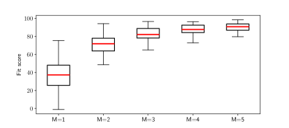
Figure 1: Values of the fit score $\mathcal{F}$ in the Monte Carlo test described in Section V-A for different orders of signature truncation $M$.

V-B Open-loop control task

We now test the performance in the tracking problem detailed in Section IV-B. We consider the system (14) with parameters $(\mu,\theta,\sigma)=(1,1,1)$, defined on the time interval $[0,1]$ that is regularly subdivided by a grid $\mathcal{D}$ of points equally spaced by a step of length $0.05$. The signature model with truncation order $M=4$ is trained with $N_{\text{train}}=40$ input-output trajectories, where the piecewise-linear inputs are generated in the same way as presented in Section V-A, but with values in the range $[0,3]$. The same mechanism is used to generate the input which, fed into the system (14), yields the desired trajectory $\bar{Z}=[0,Z_{t_{1}},\dots,Z_{T}]^{\top}$ to be tracked. We carry out the procedure detailed in Section IV-B and solve the nonlinear program (13) with IPOpt implemented in CasADi [1] and initialized on a perturbation of the true input yielding a SNR of 3.5 dB. A sample outcome of the proposed procedure is presented in Figure 2.
We assess the performance using the metric $\mathcal{F}$ defined in (15) on a Monte Carlo study of $N_{MC}=50$ runs, randomizing over training and test data-sets, as well as on the CasADi initialization. In the boxplot of Figure 3 we display the different values of fit obtained by considering signal portions of increasing size. We can notice that the performance tends to degrade in quality as the trajectory length increases, which is an expected effect given the result of Theorem 4 as well as of numerical issues in solving the nonlinear program (13).

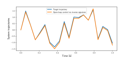
Figure 2: Sample tracking performance on experiment of Section V-B. Fit score achieved on this realization: $\mathcal{F}=90.4\%$.

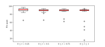
Figure 3: Tracking performance considering trajectory portions of increasing length for Monte Carlo test in Section V-B.

VI DISCUSSION

In this Section, we present some remarks on the proposed methodology, and sketch ideas for forthcoming research stemming from them.

On the choice of the dynamics model

The model as presented in (1) allows us to extend the theory outlined in Section III also to the case in which the control is a stochastic process: specifically, the theory of rough paths [16, 12] provides the theoretical tools to compute the signature for paths of bounded $p$-variation with $p>1$ (and this accounts for the Brownian motion case, for which $p=2$).
In this work we focused on piecewise-linear interpolation for sampled signals. If input paths were continuously differentiable, then the model could be also re-written as

$$\dot{Z}_{t}=f_{0}(Z_{t})+\sum_{i=1}^{d}f_{i}(Z_{t})\dot{U}_{t}^{i}.$$ (16)

These are known in the literature as impulsive systems and are very common, e.g., in Lagrangean mechanics [5]. It is possible to adapt the control algorithm of Section IV-B to smoother input signals (e.g., using higher-order splines) in order to consider systems of the form (16), possibly at the price of increasing the number of optimization variables.
The tools proposed in this paper can be extended to deal also with the more familiar model

$$dZ_{t}=f_{0}(Z_{t})dt+\sum_{i=1}^{d}f_{i}(Z_{t})U_{t}^{i}dt.$$

By defining $dV_{t}=U_{t}dt$, and obtaining $V_{t}$ with integration, the general theory outlined in Section III can still be applied by computing the signature of $X=(t,V^{1},\dots,V^{d})$. As regards the methodology presented in Section IV, this procedure would imply that one considers piecewise-constant inputs $\{U_{t}^{1},\dots,U_{t}^{d}\}$. However, this choice can be relaxed by generalizing the procedure proposed in this paper with different signal interpolation methods.

On the proposed open-loop control strategy

We start by pointing out that the algorithm proposed in Section IV-B is de facto performing the “inversion of the signature” – i.e., uses the signature to retrieve the piecewise-linear path defined on $[0,T]$ that generated it. Such a problem is still an active area of research in the case that only the signature of the whole interval $[0,T]$ is available – see the most recent work [21] and references therein. Leveraging Theorem 4, in our algorithm we are able to use all of the available information on each portion of the path, thus giving a new perspective to the problem of signature inversion.
As regards the implementation of the proposed control strategy, the current implementation in CasADI solves (13) for the example presented in Section V-B at an average total time of 31.4 ms on a 2.6 GHz 6-Core Intel Core i7 processor. The performance can be further enhanced, both in terms of speed and solution quality, by analytically computing the gradient and the Hessian for each component of $\text{vec}(\tilde{S}(\Delta))$ with respect to $\Delta$, and including them as inputs for the optimizer. The structure of the signature matrix makes such a task feasible, and this improvement will be included in the next versions of the code.

Alternative signature-based features

In this paper, we showed the theoretical soundness and the practical effectiveness of the (truncated) signature as a feature to represent output trajectories of an unknown dynamical system described by an input-affine differential equation, tackling both tasks of prediction and (open-loop) control. The proposed algorithms rely on the hypotheses that all trajectories share the same initial condition $Z_{0}=z_{0}$, and that data are noiseless, but the continuity of the solution map for (1) and Theorem 4 provide tools to generalize such a set-up.
However, the expressive power of the truncated signature comes at the price of high computational complexity. By definition (5), it results that the truncated signature of order $M$ stores $\sum_{k=0}^{M}(d+1)^{k}$ terms, and thus its computation scales as $\mathcal{O}((d+1)^{M})$: this makes its application infeasible when dealing with high-dimensional inputs. There are two alternatives to cope with this problem. The first consists in considering the log-signature, which emerges when studying deeper algebraic structures of the signature [12, Chapter 7], and provides its compressed representation – however, while its use in prediction is already possible thanks to the available computational tools [22], the extension of the control algorithm presented in Section IV-B might be nontrivial. A further alternative is given by the randomized signature [10], whose practical effectiveness in prediction has been investigated in [18], and which should be suited to deal with the control strategy presented in Section IV-B – however, the generalization to multiple initial conditions can become challenging due to the locality of the approximation.

References

- [1] Joel A. E. Andersson et al. “CasADi – A software framework for nonlinear optimization and optimal control” Publisher: Springer In Mathematical Programming Computation 11.1, 2019, pp. 1–36 DOI: 10.1007/s12532-018-0139-4
- [2] Julian Berberich, Johannes Köhler, Matthias A. Müller and Frank Allgöwer “Data-Driven Model Predictive Control With Stability and Robustness Guarantees” Conference Name: IEEE Transactions on Automatic Control In IEEE Transactions on Automatic Control 66.4, 2021, pp. 1702–1717 DOI: 10.1109/TAC.2020.3000182
- [3] Julian Berberich, Johannes Köhler, Matthias A. Müller and Frank Allgöwer “Linear Tracking MPC for Nonlinear Systems—Part II: The Data-Driven Case” Conference Name: IEEE Transactions on Automatic Control In IEEE Transactions on Automatic Control 67.9, 2022, pp. 4406–4421 DOI: 10.1109/TAC.2022.3166851
- [4] Petar Bevanda, Stefan Sosnowski and Sandra Hirche “Koopman operator dynamical models: Learning, analysis and control” In Annual Reviews in Control 52, 2021, pp. 197–212 DOI: 10.1016/j.arcontrol.2021.09.002
- [5] Alberto Bressan “Impulsive Control Systems” In Nonsmooth Analysis and Geometric Methods in Deterministic Optimal Control Springer, 1996, pp. 1–22 DOI: 10.1007/978-1-4613-8489-2˙1
- [6] Kuo-sai Chen “Integration of paths—a faithful representation of paths by non-commutative formal power series” In Transactions of the American Mathematical Society 89.2, 1958, pp. 395–407 DOI: 10.1090/S0002-9947-1958-0106258-0
- [7] Changming Cheng, Z. K. Peng, W. M. Zhang and G. Meng “Volterra-series-based nonlinear system modeling and its engineering applications: A state-of-the-art review” In Mechanical Systems and Signal Processing 87, 2017, pp. 340–364 DOI: 10.1016/j.ymssp.2016.10.029
- [8] Ilya Chevyrev and Andrey Kormilitzin “A Primer on the Signature Method in Machine Learning” arXiv:1603.03788 [cs, stat] arXiv, 2016 DOI: 10.48550/arXiv.1603.03788
- [9] Jeremy Coulson, John Lygeros and Florian Dörfler “Data-Enabled Predictive Control: In the Shallows of the DeePC” In 2019 18th European Control Conference (ECC), 2019, pp. 307–312 DOI: 10.23919/ECC.2019.8795639
- [10] Christa Cuchiero et al. “Expressive Power of Randomized Signature” In Workshop on The symbiosis of Deep Learning and Differential Equations, 2021
- [11] Adeline Fermanian “Embedding and learning with signatures” In Computational Statistics & Data Analysis 157, 2021 DOI: 10.1016/j.csda.2020.107148
- [12] Peter K. Friz and Nicolas B. Victoir “Multidimensional Stochastic Processes as Rough Paths: Theory and Applications”, Cambridge Studies in Advanced Mathematics Cambridge University Press, 2010 DOI: 10.1017/CBO9780511845079
- [13] Ben Hambly and Terry Lyons “Uniqueness for the signature of a path of bounded variation and the reduced path group” Publisher: Annals of Mathematics In Annals of Mathematics 171.1, 2010, pp. 109–167 URL: https://www.jstor.org/stable/27799199
- [14] Linbin Huang, John Lygeros and Florian Dörfler “Robust and Kernelized Data-Enabled Predictive Control for Nonlinear Systems” Conference Name: IEEE Transactions on Control Systems Technology In IEEE Transactions on Control Systems Technology 32.2, 2024, pp. 611–624 DOI: 10.1109/TCST.2023.3329334
- [15] Franz J. Kiraly and Harald Oberhauser “Kernels for Sequentially Ordered Data” In Journal of Machine Learning Research 20.31, 2019, pp. 1–45 URL: http://jmlr.org/papers/v20/16-314.html
- [16] Terry J. Lyons, Michael Caruana and Thierry Lévy “Differential Equations Driven by Rough Paths: École d’Été de Probabilités de Saint-Flour XXXIV - 2004” 1908, Lecture Notes in Mathematics Berlin, Heidelberg: Springer, 2007 DOI: 10.1007/978-3-540-71285-5
- [17] Oleksii Molodchyk and Timm Faulwasser “Exploring the Links Between the Fundamental Lemma and Kernel Regression” Conference Name: IEEE Control Systems Letters In IEEE Control Systems Letters 8, 2024, pp. 2045–2050 DOI: 10.1109/LCSYS.2024.3406053
- [18] Enea Monzio Compagnoni et al. “On the effectiveness of Randomized Signatures as Reservoir for Learning Rough Dynamics” ISSN: 2161-4407 In 2023 International Joint Conference on Neural Networks (IJCNN), 2023, pp. 1–8 DOI: 10.1109/IJCNN54540.2023.10191624
- [19] Motoya Ohnishi et al. “Signatures Meet Dynamic Programming: Generalizing Bellman Equations for Trajectory Following” Publisher: arXiv Version Number: 2 In 6th Annual Learning for Dynamics and Control Conference, 2024 DOI: 10.48550/ARXIV.2312.05547
- [20] Gianluigi Pillonetto et al. “Regularized System Identification: Learning Dynamic Models from Data”, Communications and Control Engineering Cham: Springer International Publishing, 2022 DOI: 10.1007/978-3-030-95860-2
- [21] Marco Rauscher, Alessandro Scagliotti and Felipe Pagginelli “Shortest-path recovery from signature with an optimal control approach” arXiv:2310.10619 [cs, eess, math] In arXiv:2310.10619v4, 2023 DOI: 10.48550/arXiv.2310.10619
- [22] Jeremy Reizenstein and Benjamin Graham “The iisignature library: efficient calculation of iterated-integral signatures and log signatures” arXiv:1802.08252 [cs, math] In arXiv:1802.08252, 2018 DOI: 10.48550/arXiv.1802.08252
- [23] Walter Rudin “Principles of Mathematical Analysis” Google-Books-ID: kwqzPAAACAAJ McGraw-Hill, 1976
- [24] Chris Verhoek, Patrick J. W. Koelewijn, Sofie Haesaert and Roland Tóth “Direct Data-Driven State-Feedback Control of General Nonlinear Systems” ISSN: 2576-2370 In 2023 62nd IEEE Conference on Decision and Control (CDC), 2023, pp. 3688–3693 DOI: 10.1109/CDC49753.2023.10384139
- [25] Qingsong Wen et al. “Transformers in Time Series: A Survey” ISSN: 1045-0823 In Thirty-Second International Joint Conference on Artificial Intelligence (IJCAI) 6, 2023, pp. 6778–6786 DOI: 10.24963/ijcai.2023/759
- [26] Jan C. Willems, Paolo Rapisarda, Ivan Markovsky and Bart L. M. De Moor “A note on persistency of excitation” In Systems & Control Letters 54.4, 2005, pp. 325–329 DOI: 10.1016/j.sysconle.2004.09.003