Efficient nonparametric estimators of discrimination measures with censored survival data

Abstract

Discrimination measures such as the concordance index and the cumulative-dynamic time-dependent area under the ROC-curve (AUC) are widely used in the medical literature for evaluating the predictive accuracy of a scoring rule which relates a set of prognostic markers to the risk of experiencing a particular event. Often the scoring rule being evaluated in terms of discriminatory ability is the linear predictor of a survival regression model such as the Cox proportional hazards model. This has the undesirable feature that the scoring rule depends on the censoring distribution when the model is misspecified. In this work we focus on linear scoring rules where the coefficient vector is a nonparametric estimand defined in the setting where there is no censoring. We propose so-called debiased estimators of the aforementioned discrimination measures for this class of scoring rules. The proposed estimators make efficient use of the data and minimize bias by allowing for the use of data-adaptive methods for model fitting. Moreover, the estimators do not rely on correct specification of the censoring model to produce consistent estimation. We compare the estimators to existing methods in a simulation study, and we illustrate the method by an application to a brain cancer study.

Keywords: Concordance probability, Efficient influence function, Predictive accuracy, Right-censoring, Survival data, Variable importance.

1 Introduction

Evaluating the predictive accuracy of a set of prognostic markers is an important objective of many medical studies. For example, in the brain cancer study in Section 7 the objective is to evaluate whether a cheaper tumor growth biomarker predicts survival time not worse than a more expensive tumor growth marker when accounting for established genetic risk factors. A popular metric for evaluating variable importance in a time-to-event setting is the so-called concordance-index or c-index [Harrell et al., 1982, Harrell Jr et al., 1996, Heagerty and Zheng, 2005, Pencina and D’agostino, 2004], which quantifies how well an estimated scoring rule discriminates between subjects with different event times. Considering two random subjects $(i,j)$ from the population of interest the c-index is informally defined as

$$C=Pr(score(i)\geq score(j)\mid i\text{ has event before }j),$$ (1)

where $\textit{score}(i)$ is the risk score for subject $i$. An early estimator of the c-index for survival data was proposed by Harrell Jr et al. [1996]. However, as noted by Gönen and Heller [2005] and Uno et al. [2011], the limiting value of Harell’s c-index estimator depends on the censoring distribution. To address this limitation Uno et al. [2011] develop an estimator based on inverse probability of censoring weighting (IPCW) which is consistent for a time-truncated version of (1) under independent censoring. Uno et al. [2011] use the Cox model to construct their scoring and it therefore depends on the censoring distribution if the model is not correctly specified. Gerds et al. [2013] propose an IPCW estimator that allows for marker-dependent censoring thus alleviating the independent censoring assumption of Uno et al. [2011]. Unfortunately, Gerds et al. [2013] give no large sample results of their proposed method making it hard to use for distinguishing between the predictive value of competing biomarkers such as the two in the brain cancer study in Section 7. Although IPCW estimators are simple to compute, as they only require fitting a model for the probability of censoring, they are limited in that they rely on correct specification of the censoring model to produce consistent estimation. Moreover, IPCW is generally not an efficient semiparametric method. A different approach was taken by Gönen and Heller [2005] who propose a plug-in estimator of the so-called concordance probability which is informally defined as

$$K=Pr(i\text{ has event before }j\mid score(i)\geq score(j)),$$ (2)

assuming that data are generated by a proportional hazards model. If this is not the case then their estimator will be biased, and moreover it depends on the censoring distribution in the specific study which clearly is of no scientific interest. Note than when the event time and scoring rule are both continuous and we do not truncate the event-time then the concordance measures in (1) and (2) are identical. If, as is commonly done, we restrict to a specific time horizon $\tau$ (i.e we only observe up to a given point in time) then the two measures are proportional.

As pointed out by [Blanche et al., 2019] the c-index is not proper for the evaluation of $t$-year predicted risks, i.e. it may take a higher value for a scoring rule based on a misspecified model than for a scoring rule based on a correctly specified model. They recommended instead to look at the so-called cumulative-dynamic time-dependent area under the ROC-curve ($\mbox{AUC}_{t}$) [Heagerty et al., 2000, Heagerty and Zheng, 2005, Blanche et al., 2013] that is proper in this scenario. The $\mbox{AUC}_{t}$ quantifies how well a scoring rule discriminates between subjects with different survival status at a given time point $t\leq\tau$, and is informally defined as

$$\mbox{AUC}_{t}=Pr(score(i)\geq score(j)\mid i\text{ has event before }t\text{ and }j\text{ has event after }t).$$ (3)

Frequently used estimators of the $\mbox{AUC}_{t}$ include plug-in estimators assuming that data are generated by a proportional hazards model [Chambless and Diao, 2006, Song and Zhou, 2008] and IPCW estimators [Uno et al., 2007, Hung and Chiang, 2010].

In this paper, we improve upon the foregoing approaches in several important directions. By viewing (1), (2) and (3) as model-free discrimination measures we develop debiased estimators based on the corresponding efficient influence functions. This give rise to efficient and flexible root-$n$ consistent estimators that are asymptotically model-free by enabling data-adaptive methods (e.g., machine learning). A further benefit is that the censoring mechanism can depend in an arbitrarily complex way on the considered markers and no specific working censoring model is required. To the best of our knowledge, this is the first proposal of such a method for discrimination measures in a survival setting.

The three discrimination measures mentioned above all rely on a given scoring rule, which we denote by $\beta^{T}X$ with $X$ being the available markers that we wish to use to form the scoring rule. It turns out to be important how the coefficient vector $\beta$ is chosen. We use a well defined estimand, $\beta(P)$, that does not rely on data being generated from any specific model such as the Cox-model. To estimate $\beta(P)$ we first calculate its efficient influence function and use the corresponding one-step estimator. This turns out to be crucial in order to obtain simple estimators for the three discrimination measures of interest.

This paper is organized as follows. In Section 2 we define the concordance measures more formally. In Section 3 we propose locally efficient non-parametric estimators of the truncated versions of $K$ and $C$ based on the efficient influence function and we discuss estimation of $\beta(P)$. In Section 4 we define $\mbox{AUC}_{t}$ more formally and propose an estimator based on its efficient influence function. In Section 6 we conduct a simulation study to illustrate the large sample properties of the estimators and in Section 7 we apply the proposed novel estimators to some brain cancer data where it is of importance to judge whether a cheaper biomarker has a predictive power not worse than a more expensive marker. Some final remarks are provided in Section 8. Technical derivations are relegated to the Appendix.

2 Concordance measures

Let $T$ denote the continuous failure time and $X$ the $d$-dimensional vector of markers. Let $C$ denote the censoring time so that we observe $\tilde{T}=T\wedge C$ and $\Delta=I(T\leq C)$, and assume that $T$ and $C$ are conditionally independent given $X$. Let $O=(\tilde{T},\Delta,X)$ and $Z=(T,X)$ with the latter corresponding to the case where there is no censoring which we informally refer to as full data. We observe data in the time interval $[0,\tau]$ with $\tau<\infty$. We let $N^{o}(t)=I(\tilde{T}\leq t,\Delta=1)$ denote the counting process that jumps when an event time of interest is observed, and also define $N(t)=I(T\leq t)$ corresponding to the counting process in the case without censoring.

Let $\beta(P)$ be some estimand and define the scoring rule

$$Y=\beta^{T}X,$$

that we wish to evaluate in terms of predictive power. Here $\beta$ is short for $\beta(P)$. We return to how $\beta(P)$ can be chosen. We further assume that the covariate vector $X$ contains at least one continuous covariate that we call $W$, and write $X=(V,W)$ with $V$ denoting the remaining covariates. Also,

$$\beta^{T}X=\beta_{V}^{T}V+\beta_{W}W$$

and for now assume $\beta_{W}>0$. The concordance probability of Gönen and Heller [2005] is

$$K_{\tau}(P)=P(T_{2}>T_{1},T_{1}\leq\tau\mid Y_{1}\geq Y_{2}),$$ (4)

where $T_{j}$ is shorthand notation for a draw of the event time from the population where we restrict to $Y_{j}$. In Gönen and Heller [2005], the truncation by $\tau$ is left out and the resulting concordance probability is calculated assuming that data are generated by a Cox-model which further makes estimation possible. However, without the finite maximum follow-up time $\tau$, the concordance probability is not in general identifiable. The concordance index, also known as the c-index [Harrell et al., 1982, Harrell Jr et al., 1996, Pencina and D’agostino, 2004], for survival data is, in the truncated form, given by

$$C_{\tau}(P)=P(Y_{1}\geq Y_{2}\mid T_{2}>T_{1},T_{1}\leq\tau),$$ (5)

see [Uno et al., 2011, Heagerty and Zheng, 2005]. Clearly, these two concordance measures are proportional to

$$\Psi_{\tau}(P)=P(T_{2}>T_{1},T_{1}\leq\tau,Y_{1}\geq Y_{2}),$$ (6)

in the considered setting, where both $Y$ and $T$ are continuous. Specifically,

$$K_{\tau}(P)=2\Psi_{\tau}(P)\quad\mbox{and}\quad C_{\tau}(P)=2\Psi_{\tau}(P)/\left\{1-S^{2}(\tau)\right\}.$$

In the following we develop robust nonparametric estimators of both $K_{\tau}(P)$ and $C_{\tau}(P)$ mitigated by calculating the efficient influence function of $\Psi_{\tau}(P)$. We will write $K_{\tau}$ for $K_{\tau}(P)$ and likewise for the other estimands unless we wish to stress the dependence on $P$.

3 Robust nonparametric estimators of $K_{\tau}$ and $C_{\tau}$

The key to develop the novel estimators of the two concordance measures is to calculate the efficient influence function (eif) of $\Psi_{\tau}(P)$ without any reference to a specific statistical model such as the Cox model. For $y_{j}=\beta^{T}x_{j}$, $j=1,2$, define

$$h_{\tau}(y_{1},y_{2})=\int_{0}^{\tau}S(t|y_{2})S(t|y_{1})\lambda(t|y_{1})dt,$$ (7)

where $S(t|y)=P(T>t|Y=y)$ and $\lambda(t|y)$ is the corresponding conditional hazard function. Thus,

$$\Psi_{\tau}=\int\int_{y_{1}>y_{2}}h_{\tau}(y_{1},y_{2})dF_{Y}(y_{1})dF_{Y}(y_{2}),$$

where $F_{Y}$ denotes the distribution function for $Y$. We show in the Appendix that the efficient influence function corresponding to $\Psi_{\tau}$, and based on full data, is

$$D^{*}_{\Psi_{\tau}}(Z,P)=g_{\tau}(X;P)+G_{\tau}(Z,\dot{\beta},P),$$ (8)

where

$$g_{\tau}(X;P)=\int_{-\infty}^{Y}h_{\tau}(Y,y)dF_{Y}(y)+\int_{Y}^{\infty}h_{\tau}(y,Y)dF_{Y}(y)-2\Psi_{\tau}$$

and

$$G_{\tau}(Z,\dot{\beta},P)= \int_{-\infty}^{Y}\left\{\int_{0}^{\tau}S(t|y)dM(t|Y)-\int_{0}^{\tau}S(t|y)S(t|Y)\int_{0}^{t}\frac{dM(u|Y)}{S(u|Y)}d\Lambda(t|Y)\right\}dF_{Y}(y)$$

$$-\int_{Y}^{\infty}\int_{0}^{\tau}S(t|Y)\int_{0}^{t}\frac{dM(u|Y)}{S(u|Y)}S(t|y)d\Lambda(t|y)dF_{Y}(y)+\tilde{H}(\beta)\dot{\beta}(P),$$

with $\tilde{H}(\beta)$ a constant, given in display (21) in the Appendix, and $\dot{\beta}$ is the efficient influence function of $\beta$. Further, $dM(t|Y)$ denotes the martingale (increment) corresponding to the full data counting process $N(t)$ and conditioning on $Y$, and $\Lambda(t|y)=\int_{0}^{t}\lambda(u|y)du$. The only term in the full data eif that is affected when moving to the observed data case is the term $G_{\tau}(Z,\dot{\beta},P)$. If we were willing to assume conditionally independent censoring given $Y$ then we get the wanted observed data $G_{\tau}(O,\dot{\beta},P)$ by replacing $dM(\cdot|Y)$ in $G_{\tau}(Z,\dot{\beta},P)$ with $dM^{o}(\cdot|Y)/K_{C}(\cdot|Y)$ where $dM^{o}(t|Y)$ denotes the martingale (increment) corresponding to the observed counting process $N^{o}(t)$ and conditioning on $Y$, and with $K_{C}(u\mid Y)=P(C>u|Y).$ Define $dM^{o}(t|X)$ similarly where one conditions on $X$ instead of $Y$. Under the earlier stated conditionally independent censoring assumption given $X$ we need first to rewrite $dM(v|Y)$ in terms of $dM(v|X)$; this expression is given is display (A.1.1) in the Appendix. Define further

$$dL_{\beta}(v;X)=\frac{dM^{o}(v|X)}{K_{C}(v|X)}-S(v|X)\tilde{M}(v;X)d\{\Lambda(v|X)-\Lambda(v|Y)\}+S(v|X)d\{\Lambda(v|X)-\Lambda(v|Y)\},$$

with $d\tilde{M}(v;X)=dM^{o}(v|X)/\{S(v|X)K_{C}(v|X)\}.$ Finally, this gives us the wanted efficient influence function based on the observed data and where we only assume conditional independent censoring given $X$:

$$D^{*}_{\Psi_{\tau}}(O,P)= g_{\tau}(X)+G_{\tau}(O,\dot{\beta},P),$$ (9)

where

$$G_{\tau}(O,\dot{\beta},P)= \int_{-\infty}^{Y}\left\{\int_{0}^{\tau}S(t|y)dL_{\beta}(t;X)-\int_{0}^{\tau}S(t|y)S(t|Y)\int_{0}^{t}\frac{dL_{\beta}(u;X)}{S(u|Y)}d\Lambda(t|Y)\right\}dF_{Y}(y)$$

$$-\int_{Y}^{\infty}\int_{0}^{\tau}S(t|Y)\int_{0}^{t}\frac{dL_{\beta}(u;X)}{S(u|Y)}S(t|y)d\Lambda(t|y)dF_{Y}(y)+\tilde{H}(\beta)\dot{\beta}(P).$$

In the next subsection we describe how to use the eif (9) for estimation of $\Psi_{\tau}$. Before doing so we note that the constant $\tilde{H}(\beta)$ given in display (21) in the Appendix has a complicated structure involving the density function of the covariate distribution. It is therefore desirable if the estimation procedure can avoid estimation of this constant.

3.1 One-step estimator

The one-step estimator [Kennedy, 2023] of $\Psi_{\tau}$ is in this obtained by setting the empirical mean of $D^{*}_{\Psi_{\tau}}(O,P)$ equal to zero and solve for $\Psi_{\tau}$. This will obviously depend on unknown quantities, however. To this end we replace $\beta$ with some estimator $\hat{\beta}$, which we give in a moment, and $F_{Y}$ is replaced with its empirical counterpart. Since $K_{\tau}=2\Psi_{\tau}$, this results in the following one-step estimator of the concordance probability $K_{\tau}$

$$\hat{K}_{\tau}=\frac{2}{n(n-1)}\sum_{i\neq j}I\left(\hat{\beta}^{T}X_{i}>\hat{\beta}^{T}X_{j}\right)h_{\tau}\left(\hat{\beta}^{T}X_{j},\hat{\beta}^{T}X_{i}\right)+\frac{1}{n}\sum_{i=1}^{n}G_{\tau}(O_{i},\dot{\beta},P_{n}).$$ (10)

It is interesting to note that the first term in (10) corresponds to the estimator of Gönen and Heller [2005] (GH-estimator) had we used the Cox partial likelihood estimator of $\beta$. The remaining part of (10) is a debiasing term in case the data are not generated from a Cox model (given $X$). Note also that we have used the notation $P_{n}$ to indicate that we further need to replace all other unknown quantities, such as $S(\cdot|X)$, by working estimates. We will be more specific about this later but leave it vague for now. If data were in fact generated by a Cox model and we use the Cox partial likelihood estimator of $\beta$ then the debiasing term is negligible. In the more likely case where data are not generated by the Cox model the above one-step estimator can in principle be used to correct the bias of the GH-estimator. However, we do not recommend to use this procedure as it would require estimation of the constant $\tilde{H}(\beta)$, which is not attractive due to the complicated structure of this constant. However, this can be avoided all together if we further use the one-step estimator that solves the (empirical) version of the eif corresponding to the estimand $\beta(P)$. Put in other words, by doing so, the term $\tilde{H}(\beta)\dot{\beta}(P)$ can be dropped from the above eif. Since $C_{\tau}=K_{\tau}/\left\{1-S^{2}(\tau)\right\}$ this suggest the estimator

$$\hat{C}_{\tau}=\hat{K}_{\tau}/\left[1-\{\hat{S}(\tau)\}^{2}\right],$$ (11)

where $\hat{S}(\tau)$ is its corresponding one-step estimator based on the observed data:

$$\hat{S}(t)=n^{-1}\sum_{i}S_{n}(t|X_{i})\left\{1-\int_{0}^{t}\frac{dM_{n}^{o}(u|X_{i})}{S_{n}(u|X_{i})K_{C}^{n}(u|X_{i})}\right\},$$ (12)

evaluated at $t=\tau$, and where $S_{n}(u|x)$ means an estimator of $S(u|x)$, and similarly with $dM_{n}^{o}(u|X_{i})=dN^{o}_{i}(u)-I(u\leq\tilde{T})d\Lambda_{n}(u|X_{i})$ and $K_{C}^{n}$.

3.2 The estimand $\beta(P)$ and its corresponding eif

As mentioned earlier, the GH-estimator of $K_{\tau}$ relies on the scoring rule $\check{\beta}^{T}X$, where $\check{\beta}$ is the Cox partial likelihood estimator that converges to a well defined coefficient vector $\tilde{\beta}$ even if the Cox model is not correctly specified, but $\tilde{\beta}$ has the undesirable feature that it depends on the censoring distribution in the actual study in the likely case where the Cox model is misspecified. Their proposed scoring rule may thus reflect properties of the specific censoring distribution, which is of no scientific interest. We take a different approach defining the scoring rule in the setting where there is no censoring so it only reflects the association between survival and the markers. Inspired by the assumption-lean approach by Vansteelandt and Dukes [2022], Vansteelandt et al. [2024], we propose to use the coefficient $\beta_{\tau}(P)$ defined as

$$\beta_{t}(P)=\{\mbox{var}(X)\}^{-1}\mbox{cov}[g\{S(t|X)\},X],$$ (13)

where $g$ is some pre-specified link function. If we take $g(x)=\log{\{-\log{(x)}\}}$ and if in fact $S(t|X)=\exp{\{-\Lambda_{0}(t)e^{\theta^{T}X}\}}$ (ie the Cox model is correctly specified) then $\beta_{t}(P)=\theta$, but $\beta_{t}(P)$ remains well defined otherwise. The eif of $\beta_{t}(P)$ is conveniently calculated by calculating the eif of $\beta_{2}\equiv\mbox{var}(X)$ and of $\beta_{1}\equiv\mbox{cov}[g\{S(t|X)\},X]$ separately. One can show that

$$D^{*}_{\beta_{1}}(O,P)= \left[g\{S(t|X)\}-Eg\right](X-EX)-E\left[g\{S(t|X)\}-Eg\right](X-EX)$$

$$-(X-EX)g^{\prime}\{S(t|X)\}S(t|X)\int_{0}^{t}\frac{dM^{o}(u\mid X)}{K_{C}(u|X)S(u|X)}.$$

Similarly one can develop the eif for $\mbox{var}(X)$ giving the estimator $\hat{\mbox{var}}(X)=\mathbb{P}_{n}\{(X-\mathbb{P}_{n}X)(X-\mathbb{P}_{n}X)^{T}\}$, where $\mathbb{P}_{n}$ is the empirical measure $\mathbb{P}_{n}\{v(O)\}=n^{-1}\sum_{i}v(O_{i})$. This results in the desired estimator of $\beta_{t}(P)$:

$$\hat{\beta}_{t}(P)=\{\hat{\mbox{var}}(X)\}^{-1}\mathbb{P}_{n}\biggl{(} \left[g\{S_{n}(t|X)\}-\mathbb{P}_{n}g\right](X-\mathbb{P}_{n}X)$$

$$-(X-\mathbb{P}_{n}X)g^{\prime}\{S_{n}(t|X)\}S_{n}(t|X)\int_{0}^{t}\frac{dM_{n}^{o}(u\mid X)}{K_{n}(u|X)S_{n}(u|X)}\biggr{)}$$ (14)

that solves the (empirical version) of the eif of $\beta_{t}(P)$ equal to zero.

4 Estimation of $\mbox{AUC}_{t}$

The c-index is much used in practise, but it was recently argued by [Blanche et al., 2019] that the cumulative-dynamic time-dependent area under the ROC-curve ($\mbox{AUC}_{t}$) [Heagerty et al., 2000, Heagerty and Zheng, 2005, Blanche et al., 2013] defined for all $t\leq\tau$ by

$$\mbox{AUC}_{t}=P(Y_{1}\geq Y_{2}\mid T_{1}\leq t,T_{2}>t)$$ (15)

should be preferred if the aim is to predict risk of an event for a specific time horizon, $[0,t]$, say. For the same reason, we redefine $\beta(P)$ to be $\beta_{t}(P)$. Specifically, [Blanche et al., 2019] showed that the c-index is not proper while the $\mbox{AUC}_{t}$ is proper. A proper discrimination measure takes its highest value when based on the true prediction model, see [Blanche et al., 2019] for more details on proper discrimination measures. Define

$$v_{t}(y_{1},y_{2})=\{1-S(t|y_{1})\}S(t|y_{2})$$

and

$$\Theta_{t}=P(Y_{1}\geq Y_{2},T_{1}\leq t,T_{2}>t)$$ (16)

so that $\mbox{AUC}_{t}=\Theta_{t}/[\{1-S(t)\}S(t)]$. As we know how to estimate $S(t)$ using (12), we can concentrate on the estimand $\Theta_{t}$. By similar calculations as in Section 3, we get

$$D^{*}_{\Theta_{t}}(Z,P)=\tilde{g}_{t}(X;P)+\tilde{G}_{t}(Z,\dot{\beta},P),$$

where

$$\tilde{g}_{t}(X;P)=\int_{-\infty}^{Y}v_{t}(Y,y)dF_{Y}(y)+\int_{Y}^{\infty}v_{t}(y,Y)dF_{Y}(y)-2\Theta_{t}$$

and

$$\tilde{G}_{t}(Z,\dot{\beta},P)=\left\{F_{T}(t)-F_{Y}(Y)\right\}S(t|Y)\int_{0}^{t}\frac{dM(u|Y)}{S(u|Y)}+\check{H}(\beta)\dot{\beta}$$

with $\check{H}(\beta)$ another constant (given in the Appendix) and $\dot{\beta}$ is the efficient influence function of $\beta$. This leads to the following one-step estimator of $\Theta_{t}$

$$\hat{\Theta}_{t}=\frac{1}{n(n-1)}\sum_{i\neq j}I\bigl{(}\hat{\beta}^{T}X_{i}>\hat{\beta}^{T}X_{j}\bigr{)}\hat{v}_{t}\bigl{(}\hat{\beta}^{T}X_{j},\hat{\beta}^{T}X_{i}\bigr{)}+\frac{1}{2n}\sum_{i=1}^{n}\tilde{G}_{t}(O_{i},\dot{\beta},\hat{P})$$ (17)

where $\tilde{G}_{t}(O,\dot{\beta},\hat{P})$ is obtained as in Section 3 using (A.1.1) and where the part involving the complicated constant $\check{H}(\beta)$ can be dropped again as long as we use the estimator $\hat{\beta}_{t}$ given in subsection 3.2. We thus propose the following estimator

$$\widehat{\mbox{AUC}}_{t}=\hat{\Theta}_{t}/[\{1-\hat{S}(t)\}\hat{S}(t)].$$ (18)

5 Large sample and robustness properties of proposed estimators

We will focus on the proposed estimator of $\Psi_{\tau}$ but similar results apply for all the considered estimators. If we could correctly specify all the needed (working) models to calculate the proposed estimator $\hat{K}_{\tau}$ then it would have the eif given in (9) as its influence function and in principle this could be used to estimate the asymptotic variance of the estimator by taking the empirical average of the squared influence function. We first turn, however, to the robustness properties of the estimator $\hat{K}_{\tau}$ focusing on robustness in terms of consistency.

The dominating part of the remainder term for the proposed estimator of $\beta$ in terms of consistency is

$$-\left[\mathbb{P}_{n}g\{S_{n}(t|X)\}-Eg\{S(t|X)\}\right](EX-\mathbb{P}_{n}X)$$

$$-E\bigl{[}g^{\prime}\{S_{n}(t|X)\}S_{n}(t|X)(EX-\mathbb{P}_{n}X)\int_{0}^{t}\frac{\{K_{n}(u|X)-K(u|X)\}S(u|X)}{H_{n}(u|X)}d\{\Lambda_{n}-\Lambda\}(u\mid X)\bigr{]}.$$

The remainder term corresponding to the proposed estimator of $\Psi_{\tau}$with full data (ie without censoring) is

$$R_{n}^{\Psi_{\tau}}=-\int\int_{y_{1}>y_{2}}\{S_{n}(t|y_{2})-S(t|y_{2})\}d\{F_{T}^{n}(t|y_{1})-F_{T}(t|y_{1})\}dF_{Y}(y_{1})dF_{Y}(y_{2})+o_{p}(n^{-1/2}),$$

where we define $dF_{T}(t|y)=S(t|y)d\Lambda(t|y)$. In the observed data case we get the same term plus some additional terms that all involve

$$dG_{n}(u|X) =\biggl{(}\frac{K_{C}^{n}-K_{C}}{K_{C}^{n}}\biggr{)}(u|X)\{d\Lambda_{n}(u|X)-d\Lambda(u|X)\},$$

see the Appendix for more details. Hence, we can conclude, assuming the needed empirical quantities are estimated using estimator that converge at rate faster that $n^{1/4}$, that the remainder term is $o_{p}(n^{-1/2})$.

We thus get that the influence function is the efficient influence function, which in turn means that the proposed estimator is efficient. However, we do not recommend to use the efficient influence function to estimate the variability of the proposed estimator as that would involve estimation of the covariates density function as the constant (21) would reappear. Instead we propose to use the nonparametric bootstrap approach to estimate the variability. This means that both estimation and inference can be carried out without having to estimate the density function of the covariates.

6 Simulation studies

The aim of the simulation studies is to illustrate the theoretical properties of the proposed estimators. In Section 6.2 we compare the proposed estimators to existing methods under different data-generating mechanisms and model misspecifications. In Section 6.3 we demonstrate the finite sample coverage of the nonparametric bootstrap confidence intervals. R-code to replicate the simulation studies is available in the supplementary materials.

6.1 Simulation scenarios

We simulate a vector of markers $X=(X_{1},X_{2})$ with $X_{1}\sim\text{binom}(0.5)$ and $X_{2}\sim N(0,1)$, and we consider the following data-generating schemes for the event times and the censoring times.

Scenario 1

:

• Event times are generated from a proportional hazards model with Weibull baseline hazard $\lambda(t\mid X)=k\lambda^{-1}(t/\lambda)^{k-1}\exp(\beta^{T}X)$ for $k=2$, $\lambda=0.1$ and $\beta=(\text{log}(0.5),\text{log}(2))$.

• Censoring times are generated from a proportional hazards model with Weibull baseline hazard $\lambda_{C}(t\mid X_{1})=k_{C}\lambda_{C}^{-1}(t/\lambda_{C})^{k_{C}-1}\exp(\gamma_{1}X_{1}+\gamma_{2}X_{2})$ with $k_{C}=1$, $\lambda_{C}=0.1$ and $\gamma=(\text{log}(0.25),\text{log}(0.75))$.

Scenario 2

:

• Event times are generated as in Scenario 1.

• Censoring times are generated from a proportional hazards model with Weibull baseline hazard $\lambda_{C}(t\mid X_{1})=k_{C}\lambda_{C}^{-1}(t/\lambda_{C})^{k_{C}-1}\exp(\gamma_{1}X_{1}+\gamma_{2}X_{2}+\gamma_{3}X_{1}X_{2}+\gamma_{4}X_{2}^{2}+\gamma_{5}X_{1}X_{2}^{2})$ with $k_{C}=1$, $\lambda_{C}=0.1$ and $\gamma=(\log(1.5),\log(2),\log(0.25),\log(0.75),\log(0.25))$.

Scenario 3

:

• Event times are generated from a non-proportional hazards model with $\lambda(t\mid X)=(1-X_{1})k\lambda^{-1}(t/\lambda)^{k-1}\exp(\beta^{T}X)+X_{1}k\lambda^{-1}(t/\lambda)^{k-1}\exp(I(X_{2}<0)\beta_{1}+\beta_{2}X_{2})$ for $k=2$, $\lambda=0.1$ and $\beta=(\text{log}(0.5),\text{log}(2))$.

• Censoring times are generated as in Scenario 1.

In Sscenarios 1 and 3 the censoring rate is approximately 40% and in Scenario 2 the censoring rate is approximately 50%.

6.2 Simulation study 1: comparison with existing methods

For each of the three data-generating mechanisms described above we simulate data with a sample size of $n\in\{100,300,500,1000,2000,3000\}$. The truncation time for the concordance probability and the c-index, and the landmark time for the AUC was set to $\tau=t=8$. The true values in Scenario 1 and Scenario 2 are $K_{\tau,0}=0.446$, $C_{\tau,0}=0.697$ and $\mbox{AUC}_{t,0}=0.745$, and the true values in Scenario 3 (with $\beta$ defined as in (13)) are $K_{\tau,0}=0.499$, $C_{\tau,0}=0.708$ and $\mbox{AUC}_{t,0}=0.772$.

In Figure 1 we compare various estimators of the concordance probability $K_{\tau}$. For each simulated data set we compute a truncated version of the Gönen & Heller estimator (GH), the one-step estimator defined in Equation (10), as well as the plug-in estimator of the concordance probability which is equal to (10) without the debiasing term. Similarly, in Figure 2 we compare various estimators of the c-index. We compute the IPCW estimator of Uno et al. [2011] (IPCW-Uno), an IPCW estimator allowing for marker-dependent censoring inspired by Gerds et al. [2013] where the working model for the censoring distribution is a Cox regression adjusted for main effects of $X_{1}$ and $X_{2}$ (IPCW-Cox), the one-step estimator defined in Equation (11) and a corresponding plug-in estimator. Finally, in Figure 3 we compare various estimators of the AUC. For each data-set we compute the IPCW estimator of Uno et al. [2007], Hung and Chiang [2010] (IPCW-Uno), an IPCW estimator allowing for marker-dependent censoring inspired by Blanche et al. [2013] where the working model for the censoring distribution is a Cox regression adjusted for main effects of $X_{1}$ and $X_{2}$ (IPCW-Cox), the one-step estimator defined in Equation (18) and a corresponding plug-in estimator. To estimate the working models for the one-step and the plug-in estimators we considered both Cox proportional hazards regression and survival random forest using the survival_forest function from the grf package [Tibshirani et al., 2023]. Particularly, for the plug-in-Cox and one-step-Cox estimators the working model for the survival and censoring distributions is a Cox regression adjusted for main effects of $X_{1}$ and $X_{2}$. We computed one-step estimators based on survival random forests without cross-fitting (one-step-SRF) and with 5-fold cross-fitting (one-step-SRF-CF). Note that for the GH, IPCW-Uno and IPCW-Cox estimators the scoring rule is the linear predictor of a Cox PH model. For the plug-in and one-step estimators, the scoring rule is constructed using the assumption lean coefficient in (13). We repeated this 1000 times and we computed the absolute bias scaled by $\sqrt{n}$, the empirical standard deviation (sd) scaled by $\sqrt{n}$, and the mean square error (mse) scaled by $n$.

Figure 1: Simulation results for comparing estimators of $K_{\tau}$. Row 1 is absolute bias times $\sqrt{n}$, row 2 is empirical standard deviation times $\sqrt{n}$, row 3 is mean square error times $n$.

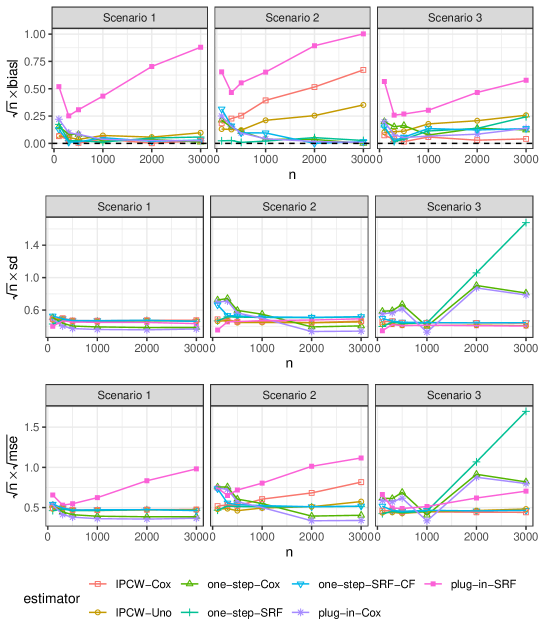
Figure 2: Simulation results for comparing estimators of $C_{\tau}$. Row 1 is absolute bias times $\sqrt{n}$, row 2 is empirical standard deviation times $\sqrt{n}$, row 3 is mean square error times $n$.

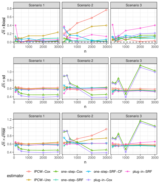
Figure 3: Simulation results for comparing estimators of $\mbox{AUC}_{\tau}$. Row 1 is absolute bias times $\sqrt{n}$, row 2 is empirical standard deviation times $\sqrt{n}$, row 3 is mean square error times $n$.

We see that, as expected, the GH, IPCW-Cox and plug-in-Cox estimators perform well in Scenario 1 where data is generated from a Cox proportional hazards model and the censoring model is correctly specified. The IPCW-Uno estimator is biased across all three scenarios as the independent censoring assumption is violated, and when the censoring model is misspecified as in Scenario 2 the scaled bias of the IPCW-Cox does not tend to zero. Unsurprisingly the one-step-Cox estimator is robust to misspecification of the censoring model in Scenario 2, but not misspecification of the model for the survival distribution in Scenario 3. In general the scaled bias of the plug-in-SRF estimator does not tend to zero due to the slower convergence rate of the survival random forest algorithm. Importantly, the simulation studies demonstrate that the scaled bias of one-step estimator based on survival random forest stabilizes to a small value across all three scenarios. The bias of the cross-fitted estimator is generally larger than the bias of the non cross-fitted estimator for the smaller sample sizes, but tends to zero faster than $1/\sqrt{n}$. The cross-fitting appears particularly important in Scenario 3 where the variability of the non cross-fitted estimator is increasing drastically with sample size.

6.3 Simulation study 2: finite sample coverage

We simulate data from the data generating mechanism in Scenario 1 with a sample size of $n\in\{100,300,500\}$. For each simulated data set we compute the one-step estimator of the concordance probability $\hat{K}_{\tau}$ defined in Equation (10) , the one-step estimator of the c-index $\hat{C}_{\tau}$ defined in Equation (11) and the one-step estimator of $\mbox{AUC}_{t}$ defined in (18). As above the truncation time for the concordance probability and the c-index was set to $\tau=8$ and the landmark time for the AUC was set to $t=8$.

To estimate the working models we considered both correctly specified Cox proportional hazards regression using the cox.aalen function from the timereg package [Scheike and Zhang, 2011, Scheike and Martinussen, 2006] (Table 1) and survival random forest using the survival_forest function from the grf package [Tibshirani et al., 2023] (Table 2). This was repeated 1000 times and we computed the bias, empirical standard deviation (sd), the bootstrap standard error based on 500 replications (se) and the coverage of a 95% Wald-type confidence interval (cov).

Table 1: Simulation results for Cox regression. bias is the average bias across simulations ($\times 100$); sd is the empirical standard deviation ($\times 100$); se is the average standard error across simulations ($\times 100$); cov is the coverage of a 95% Wald type confidence interval ($\times 100$). Each entry is based on 1000 replicates.

	n	100	300	500
$\hat{K}_{\tau}$	bias	-1.48	-0.59	-0.27
	sd	5.30	2.93	2.26
	se	5.37	3.04	2.32
	cov	94.6	96.1	95.4
$\hat{C}_{\tau}$	bias	-1.53	-0.49	-0.37
	sd	5.07	2.52	1.80
	se	5.14	2.66	1.96
	cov	94.8	95.5	95.7
$\widehat{\mbox{AUC}}_{t}$	bias	0.17	0.07	-0.02
	sd	6.33	2.98	2.14
	se	6.59	3.17	2.32
	cov	94.2	94.7	96.7

In Table 1 we see that, unsurprisingly, when the working models are estimated using a correctly specified Cox model the one-step estimators are unbiased and the average estimated standard error closely approximates the empirical standard deviation. The Wald-type 95% confidence interval exhibits a coverage close to the nominal level.

Table 2: Simulation results for survival random forest without cross-fitting. bias is the average bias across simulations ($\times 100$); sd is the empirical standard deviation ($\times 100$); se is the average standard error across simulations ($\times 100$); cov is the coverage of a 95% Wald type confidence interval ($\times 100$). Each entry is based on 1000 replicates.

	n	100	300	500
$\hat{K}_{\tau}$	bias	-1.52	-0.43	-0.18
	sd	4.90	2.98	2.36
	se	4.89	2.98	2.39
	cov	94.1	94.8	95.3
$\hat{C}_{\tau}$	bias	-1.74	-0.14	-0.11
	sd	4.27	2.76	2.07
	se	4.35	2.71	2.23
	cov	93.2	93.9	95.0
$\widehat{\mbox{AUC}}_{t}$	bias	-1.37	-0.05	-0.07
	sd	5.38	3.40	2.58
	se	5.39	3.33	2.60
	cov	94.3	93.9	95.5

In Table 2 we see that when the working models are estimated using survival random forest the estimators remain unbiased. The average estimated standard error closely approximates the empirical standard deviation and the confidence interval exhibits a coverage close to the nominal level, though slightly anti-conservative for the smaller sample size ($n=100$).

7 Empirical study: Brain Tumor Data

This study consist of data from a total of 105 glioma patients. At first suspicion of tumor growth a simultaneous PET/MRI brain scan was made for each patient. Tumor volume determined by the PET and MRI is called FET-VOL and BV-VOL, respectively. Besides this, there is also information about a binary genetic marker ‘methyl’ which is a well established predictor. Figure 4 shows the Kaplan-Meier curves of the survival probability and the censoring probability, as well as the number of people at risk and the cumulative number of events.

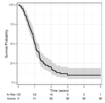
(a)

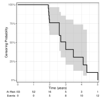
(b)

Figure 4: Brain tumor data. Kaplan-Meier estimates of (a) the survival probability and (b) the censoring probability. The numbers at risk and cumulative number of events are given below.

The primary aim of the study was to investigate whether the cheaper biomarker BV-VOL is as good as the more expensive biomarker FET-VOL in terms of discriminatory ability concerning survival within the first to two year after suspicion of tumor growth. We therefore compare the discriminatory power of the scoring rules based on (A) FET-VOL and methyl; and (B) BV-VOL and methyl.

Table 3 shows the estimated estimated $C_{\tau}$ and $K_{\tau}$ for $\tau=2$ using scoring rules (A) and (B), and for each of these using Cox proportional hazards regression and survival random forest regression, respectively, to estimate the needed predicted survival and censoring probabilities.

Table 3: Brain tumor data. One step estimates ($\times 100$) of $\mbox{C}_{\tau}$ and $\mbox{K}_{\tau}$ for $\tau=2$ with 95% confidence intervals.

	Cox PH			SRF
	score A	score B		score A	score B
$\hat{\mbox{C}}_{\tau}$	64.1	68.6		65.0	68.6
	(54.5; 73.6)	(64.0; 73.3)		(58.9; 71.1)	(64.0; 73.3)
$\hat{\mbox{K}}_{\tau}$	61.3	65.7		62.1	65.6
	(52.3; 70.3)	(61.4; 70.0)		(56.2; 68.0)	(61.5; 69.8)

Figure 5 shows the estimated $\mbox{AUC}_{t}$ as a function of time for $t\leq\tau$ using scoring rules (A) and (B). As before estimation of the predicted survival and censoring probabilities is based on Cox proportional hazards regression and survival random forest regression, respectively. Also shown in Table 3 and Figure 5 are the pointwise 95% Wald-type confidence intervals where the standard errors are estimated using nonparametric bootstrap with $1000$ replication.

(a)

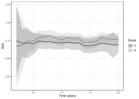
(b)

Figure 5: Brain tumor data. One-step estimates of $\mbox{AUC}_{t}$ versus time with pointwise 95% confidence intervals and working models based on (a) Cox proportional hazards regression, (b) survival random forest regression.

It is seen from all of the proposed discriminatory measures that the discriminatory ability of score B was at least as good as score A both in terms of overall risk and $t$-year predicted risk.

8 Concluding remarks

In this paper we proposed novel debiased estimators of the c-index, the concordance probability, and the $t$-year area under the receiver operating characteristic (ROC) curve ($\mbox{AUC}_{t}$). As demonstrated in our simulation study, the proposed estimators have many desirable properties including (i) do not require data to be generated from a specific model such as the Cox model (ii) robustness to misspecfication of the censoring model and (iii) allow for the use of data-adaptive methods for model fitting. We illustrated the use of the estimators by an application to data from a study on brain tumor growth where we compared the discriminatory power of a score (A) which included the tumor growth biomarker FET-VOL and the genetic marker methyl as predictors to a score (B) with the tumor growth biomarker BV-VOL and the genetic marker methyl as predictors. The analysis showed that the discriminatory ability of score B was at least as good as score A.

A key step in the development of the proposed estimators was to apply an estimator of the estimand $\beta_{t}(P)$ that solves (the empirical version) of its corresponding eif equal to zero as we could then avoid estimation of the density function of the covariate distribution. The specific choice of the estimand $\beta_{t}(P)$ may be less crucial, however, and others may be pursued as well. We leave this for future work.

Appendix A

A.1 Derivation of the efficient influence function

In this section we derive the efficient influence function (eif) of the target parameters in (6), (16) and (13). There are many ways of deriving efficient influence functions. As described by e.g. Hines et al. [2022] and Kennedy [2023] we will derive the eif by computing the Gâteaux derivative of the parameter in the direction of a point mass contamination. Specifically we will compute the directional derivative

$$\frac{d}{d\varepsilon}\bigg{|}_{\varepsilon=0}\Psi(P_{\varepsilon}),$$

where $P_{\varepsilon}=(1-\varepsilon)P+\varepsilon\delta_{\tilde{z}}$ and $\delta_{\tilde{z}}$ is the Dirac measure at $Z=\tilde{z}$. We will start by deriving the eif based on full data and then use Tsiatis [2006] Theorem 10.1 and Theorem 10.4 to map the full-data eif to the observed-data eif.

A.1.1 Efficient influence function of $\Psi_{\tau}(P)$

We first note that

$$F_{Y}(y)=P(Y\leq y)=\int\int^{\frac{y-\beta_{V}^{T}v}{\beta_{W}}}f_{W|V}(w\mid v)dwf_{V}(v)dv,$$

so that by the chain rule and the Leibniz integral rule we have that the Gâteaux derivative is

$$\frac{d}{d\varepsilon}\bigg{|}_{\varepsilon=0}F_{Y,\varepsilon}(y)= F_{W|V}\left(\frac{y-\beta_{V}^{T}\tilde{v}}{\beta_{W}}\right)-F_{Y}(y)+H(\beta;y)\dot{\beta}(P)+I(\beta_{V}^{T}\tilde{v}+\beta_{W}\tilde{w}\leq y)$$

$$-F_{W|V}\left(\frac{y-\beta_{V}^{T}\tilde{v}}{\beta_{W}}\right)$$

$$= I(\tilde{y}\leq y)-F_{Y}(y)+H(\beta;y)\dot{\beta}(P),$$ (19)

where

$$H(\beta;y)=-\frac{1}{\beta_{W}}\int f_{W|V}\left(\frac{y-\beta_{V}^{T}v}{\beta_{W}}\right)\left[v^{T},\frac{y-\beta_{V}^{T}v}{\beta_{W}}\right]f_{V}(v)dv,$$ (20)

is a non-stochastic constant and $\dot{\beta}(P)$ is the influence function for $\beta$.

We further note that

$$\frac{d}{d\varepsilon}\bigg{|}_{\varepsilon=0}\Lambda_{\varepsilon}(t\mid y)=\frac{\delta_{\tilde{y}}(y)}{f_{Y}(y)}\int_{0}^{t}\frac{dM(u\mid y)}{S(u\mid y)},$$

and that

$$\frac{d}{d\varepsilon}\bigg{|}_{\varepsilon=0}S_{\varepsilon}(t\mid y)=-\frac{\delta_{\tilde{y}}(y)}{f_{Y}(y)}S(t\mid y)\int_{0}^{t}\frac{dM(u\mid y)}{S(u\mid y)},$$

so that by the chain rule

$$\frac{d}{d\varepsilon}\bigg{|}_{\varepsilon=0}h_{\tau,\varepsilon}(y_{1},y_{2})= \int_{0}^{\tau}\frac{d}{d\varepsilon}\bigg{|}_{\varepsilon=0}S_{\varepsilon}(t\mid y_{2})S(t\mid y_{1})d\Lambda(t\mid y_{1})+\int_{0}^{\tau}S(t\mid y_{2})\frac{d}{d\varepsilon}\bigg{|}_{\varepsilon=0}S_{\varepsilon}(t\mid y_{1})d\Lambda(t\mid y_{1})$$

$$+\int_{0}^{\tau}S(t\mid y_{2})S(t\mid y_{1})\frac{d}{d\varepsilon}\bigg{|}_{\varepsilon=0}d\Lambda_{\varepsilon}(t\mid y_{1})$$

$$= -\frac{\delta_{\tilde{y}}(y_{2})}{f_{Y}(y_{2})}\int_{0}^{\tau}S(t\mid y_{2})\int_{0}^{t}\frac{dM(u\mid y_{2})}{S(u\mid y_{2})}S(t\mid y_{1})d\Lambda(t\mid y_{1})$$

$$-\frac{\delta_{\tilde{y}}(y_{1})}{f_{Y}(y_{1})}\int_{0}^{\tau}S(t\mid y_{2})S(t\mid y_{1})\int_{0}^{t}\frac{dM(u\mid y_{1})}{S(u\mid y_{1})}d\Lambda(t\mid y_{1})$$

$$+\frac{\delta_{\tilde{y}}(y_{1})}{f_{Y}(y_{1})}\int_{0}^{\tau}S(t\mid y_{2})dM(t\mid y_{1}).$$

Then

$$\frac{d}{d\varepsilon}\bigg{|}_{\varepsilon=0}\Psi_{\tau}(P_{\varepsilon})= \int\int_{y_{1}>y_{2}}h_{\tau}(y_{1},y_{2})dF_{Y}(y_{1})\frac{d}{d\varepsilon}\bigg{|}_{\varepsilon=0}F_{Y,\varepsilon}(y_{2})+\int\int_{y_{1}>y_{2}}h_{\tau}(y_{1},y_{2})\frac{d}{d\varepsilon}\bigg{|}_{\varepsilon=0}F_{Y,\varepsilon}(y_{1})dF_{Y}(y_{2})$$

$$+\int\int_{y_{1}>y_{2}}\frac{d}{d\varepsilon}\bigg{|}_{\varepsilon=0}h_{\tau,\varepsilon}(y_{1},y_{2})dF_{Y}(y_{1})dF_{Y}(y_{2})$$

$$= \int I(y<\tilde{y})h_{\tau}(\tilde{y},y)dF_{Y}(y)+\int I(y>\tilde{y})h_{\tau}(y,\tilde{y})dF_{Y}(y)+\tilde{H}(\beta)\dot{\beta}(P)-2\Psi_{\tau}(P)$$

$$-\int I(y>\tilde{y})\int_{0}^{\tau}S(t|\tilde{y})\int_{0}^{t}\frac{dM(u|\tilde{y})}{S(u|\tilde{y})}S(t|y)d\Lambda(t|y)dF_{Y}(y)$$

$$-\int I(y<\tilde{y})\left\{\int_{0}^{\tau}S(t|y)S(t|\tilde{y})\int_{0}^{t}\frac{dM(u|\tilde{y})}{S(u|\tilde{y})}d\Lambda(t|\tilde{y})-\int_{0}^{\tau}S(t|y)dM(t|\tilde{y})\right\}dF_{Y}(y),$$

where

$$\tilde{H}(\beta)=\int I(y<\tilde{y})h_{\tau}(\tilde{y},y)H(\beta;y)dF_{Y}(y)+\int I(y>\tilde{y})h_{\tau}(y,\tilde{y})H(\beta;y)dF_{Y}(y).$$ (21)

with $H(\beta;y)$ defined in (20).

Hence the eif based on full data is

$$D^{*}_{\Psi_{\tau}}(Z)(P)= \int I(y<Y)h_{\tau}(Y,y)dF_{Y}(y)+\int I(y>Y)h_{\tau}(y,Y)dF_{Y}(y)+\tilde{H}(\beta)\dot{\beta}(P)-2\Psi_{\tau}(P)$$

$$-\int I(y>Y)\int_{0}^{\tau}S(t|Y)\int_{0}^{t}\frac{dM(u|Y)}{S(u|Y)}S(t|y)d\Lambda(t|y)dF_{Y}(y)$$

$$-\int I(y<Y)\left\{\int_{0}^{\tau}S(t|y)S(t|Y)\int_{0}^{t}\frac{dM(u|Y)}{S(u|Y)}d\Lambda(t|Y)-\int_{0}^{\tau}S(t|y)dM(t|Y)\right\}dF_{Y}(y).$$

By Tsiatis [2006] formula (10.76) we can map the eif based on full data to the eif based on observed data using the relation

$$D_{\Psi_{\tau}}^{*}(O)(P)=\frac{\Delta D^{*}_{\Psi_{\tau}}(Z)(P)}{K_{C}(\tilde{T}\wedge t\mid X)}+\int\frac{E\{D^{*}_{\Psi_{\tau}}(Z)(P)\mid T\geq u,X\}}{{K_{C}(u\mid X)}}dM_{C}(u\mid X),$$ (22)

where $dM_{C}(t\mid X)$ is the martingale (increment) corresponding to the censoring counting process $N_{C}(t)=I(\tilde{T}\leq t,\Delta=0)$ conditioning on $X$.

We note that the martingale increment $dM(t\mid Y)$ can be written in terms of the martingale increment $dM(t\mid X)$ as follows

$$dM(t\mid Y)= dN(t)-I(T\geq t)d\Lambda(t\mid Y)$$

$$= dN(t)-I(T\geq t)d\Lambda(t\mid X)+I(T\geq t)\left\{d\Lambda(t\mid X)-d\Lambda(t\mid Y)\right\}$$

$$= dM(t\mid X)+I(T\geq t)\left\{d\Lambda(t\mid X)-d\Lambda(t\mid Y)\right\}$$

$$= dM(t\mid X)-S(t\mid X)\int_{0}^{t}\frac{dM(u\mid X)}{S(u\mid X)}\left\{d\Lambda(t\mid X)-d\Lambda(t\mid Y)\right\}$$

$$+S(t\mid X)\left\{d\Lambda(t\mid X)-d\Lambda(t\mid Y)\right\},$$ (23)

where in the last equality we have used that

$$I(T\geq t)=I(T\geq t)-S(t\mid X)+S(t\mid X)=S(t\mid X)-S(t\mid X)\int_{0}^{t}\frac{dM(u\mid X)}{S(u\mid X)}.$$

Moreover for any function $h_{\beta}(u,X)$

$$\begin{split}\frac{\Delta\int h_{\beta}(u,X)dM(u\mid X)}{K_{C}(U\mid X)}&+\int\frac{dM_{C}(u\mid X)}{K_{C}(u\mid X)}E\left\{\int h_{\beta}(u,X)dM(u\mid X)\mid T\geq u,X\right\}\\ &=\int\frac{h_{\beta}(v,X)}{K_{C}(v\mid X)}dM^{o}(v\mid X).\end{split}$$ (24)

We refer to Lu and Tsiatis [2008] Lemma A.2 for a proof of this.

Combining (A.1.1) and (24) we can write the eif based on observed data in (22) as

$$D_{\Psi_{\tau}}^{*}(O)(P)= \int I(y<Y)h_{\tau}(Y,y)dF_{Y}(y)+\int I(y>Y)h_{\tau}(y,Y)dF_{Y}(y)+\tilde{H}(\beta)\dot{\beta}(P)-2\Psi_{\tau}(P)$$

$$-\int I(y>Y)\int_{0}^{\tau}S(t|Y)\int_{0}^{t}\frac{dL_{\beta}(u;X)}{S(u|Y)}S(t|y)d\Lambda(t|y)dF_{Y}(y)$$

$$-\int I(y<Y)\left\{\int_{0}^{\tau}S(t|y)S(t|Y)\int_{0}^{t}\frac{dL_{\beta}(u;X)}{S(u|Y)}d\Lambda(t|Y)-\int_{0}^{\tau}S(t|y)dL_{\beta}(t;X)\right\}dF_{Y}(y),$$ (25)

where

$$dL_{\beta}(v;X)= \frac{dM^{o}(v|X)}{K_{C}(v|X)}-S(v|X)\int_{0}^{v}\frac{dM^{o}(u|X)}{S(u\mid X)K_{C}(u|X)}d\{\Lambda(v|X)-\Lambda(v|Y)\}$$

$$+S(v|X)d\{\Lambda(v|X)-\Lambda(v|Y)\}.$$

A.1.2 Efficient influence function of $\Theta_{t}(P)$

Note that

$$\frac{d}{d\varepsilon}\bigg{|}_{\varepsilon=0}v_{t,\varepsilon}(y_{1},y_{2})= -\frac{d}{d\varepsilon}\bigg{|}_{\varepsilon=0}S_{\varepsilon}(t\mid y_{1})S(t\mid y_{2})+\left\{1-S(t\mid y_{1})\right\}\frac{d}{d\varepsilon}\bigg{|}_{\varepsilon=0}S_{\varepsilon}(t\mid y_{2})$$

$$= \frac{\delta_{\tilde{y}}(y_{1})}{f_{Y}(y_{1})}S(t\mid y_{1})\int_{0}^{t}\frac{dM(u\mid y_{1})}{S(u\mid y_{1})}S(t\mid y_{2})$$

$$-\left\{1-S(t\mid y_{1})\right\}\frac{\delta_{\tilde{y}}(y_{2})}{f_{Y}(y_{2})}S(t\mid y_{2})\int_{0}^{t}\frac{dM(u\mid y_{2})}{S(u\mid y_{2})}.$$

Then by the chain rule and (A.1.1) we have

$$\frac{d}{d\varepsilon}\bigg{|}_{\varepsilon=0}\Theta_{t}(P_{\varepsilon})= \int I(y<\tilde{y})v_{t}(\tilde{y},y)dF_{Y}(y)+\int I(y>\tilde{y})v_{t}(y,\tilde{y})dF_{Y}(y)-2\Theta_{t}(P)$$

$$+\int I(y<\tilde{y})S(t\mid y)S(t\mid\tilde{y})\int_{0}^{t}\frac{dM(u\mid\tilde{y})}{S(u\mid\tilde{y})}dF_{Y}(y)$$

$$-\int I(y>\tilde{y})v_{t}(y,\tilde{y})\int_{0}^{t}\frac{dM(u\mid\tilde{y})}{S(u\mid\tilde{y})}dF_{Y}(y)+\bar{H}(\beta)\dot{\beta}(P)$$

$$= \int I(y<\tilde{y})v_{t}(\tilde{y},y)dF_{Y}(y)+\int I(y>\tilde{y})v_{t}(y,\tilde{y})dF_{Y}(y)-2\Theta_{t}(P)$$

$$+\left\{F_{T}(t)-F_{Y}(\tilde{y})\right\}S(t\mid\tilde{y})\int_{0}^{t}\frac{dM(u\mid\tilde{y})}{S(u\mid\tilde{y})}+\bar{H}(\beta)\dot{\beta}(P),$$

where

$$\check{H}(\beta)=\int I(y<\tilde{y})v_{t}(\tilde{y},y)H(\beta;y)dF_{Y}(y)+\int I(y>\tilde{y})v_{t}(y,\tilde{y})H(\beta;y)dF_{Y}(y).$$ (26)

Hence the eif under full data is

$$D_{\Theta_{t}}^{*}(Z)(P)= \int I(y<Y)v_{t}(Y,y)dF_{Y}(y)+\int I(y>Y)v_{t}(y,Y)dF_{Y}(y)-2\Theta_{t}(P)$$

$$+\left\{F_{T}(t)-F_{Y}(Y)\right\}S(t\mid Y)\int_{0}^{t}\frac{dM(u\mid Y)}{S(u\mid Y)}+\bar{H}(\beta)\dot{\beta}(P).$$

It follows from Tsiatis [2006] equation (10.76) and (A.1.1) and (24) that the eif under observed data is

$$D_{\Theta_{t}}^{*}(O)(P)= \int I(y<Y)v_{t}(Y,y)dF_{Y}(y)+\int I(y>Y)v_{t}(y,Y)dF_{Y}(y)-2\Theta_{t}(P)$$

$$+\left\{F_{T}(t)-F_{Y}(Y)\right\}S(t\mid Y)\int_{0}^{t}\frac{dL_{\beta}(u;X)}{S(u\mid Y)}+\bar{H}(\beta)\dot{\beta}(P).$$ (27)

A.2 Second order remainder term and robustness properties

We focus on the estimand $\Psi_{\tau}$, and the goal is to investigate the robustness properties of the proposed estimator of $\Psi_{\tau}$ in terms of consistency as we have already pointed out that we will not use the influence function for inference anyway. In order to study the robustness properties of $\Psi_{\tau}$ we consider the von Mises expansion

$$\Psi_{\tau}(P_{n})-\Psi_{\tau}(P)= -E\left\{D^{*}_{\Psi_{\tau}}(Z)(P_{n})\right\}+R_{n}^{\Psi_{\tau}}$$

$$= \mathbb{P}_{n}D^{*}_{\Psi_{\tau}}(Z)(P)$$ (28)

$$-\mathbb{P}_{n}D^{*}_{\Psi_{\tau}}(Z)(P_{n})$$ (29)

$$+(\mathbb{P}_{n}-P)\left\{D^{*}_{\Psi_{\tau}}(Z)(P_{n})-D^{*}_{\Psi_{\tau}}(Z)(P)\right\}$$ (30)

$$+R_{n}^{\Psi_{\tau}},$$ (31)

where $R_{n}^{\Psi_{\tau}}=E\left\{D^{*}_{\Psi_{\tau}}(Z)(P_{n})\right\}+\Psi_{\tau}(P_{n})-\Psi_{\tau}(P)$.

The term in (28) is asymptotically normally distributed by the Central Limit Theorem. The term in (29) is the so-called ‘plug-in bias’ or first order bias term. The one-step estimator $\Psi_{\tau}(P_{n})+\frac{1}{n}\sum_{i=1}^{n}D^{*}_{\Psi_{\tau}}(Z_{i})(P_{n})$ accounts for this bias by construction. We need both the empirical process term in (30) and the second order remainder in (31) to be $o_{p}(1)$ for the one-step estimator to be consistent. The empirical process term can be controlled by either Donsker class conditions [van der Vaart, 2000] or sample splitting [Chernozhukov et al., 2018]. We analyze the second order remainder term further below. However, we study first the large sample properties of the proposed estimator of $\beta_{t}(P)$.

A.2.1 Large sample properties of $\beta_{t}(P)$

We let $\beta_{2}=\mbox{var}(X)$ and of $\beta_{1}=\mbox{cov}[g\{S(t|X)\},X]$ separately. The efficient influence function of $\beta_{t}(P)$ is easily worked out and forms the basis for efficient estimation of $\beta_{t}(P)$. The eif can be constructed based on the following facts.

$$\mbox{EIF}[Eg\{S(t|X)\}X\}] =\left[g^{\prime}\{S(t|X)\}\{I(T>t)-S(t|X)\}+g\{S(t|X)\}\right]X-Eg\{S(t|X)\}X$$

$$\mbox{EIF}[Eg\{S(t|X)\}] =g^{\prime}\{S(t|X)\}\{I(T>t)-S(t|X)\}+g\{S(t|X)\}-Eg\{S(t|X)\}$$

and the $I(T>t)-S(t|X)$ is changed to

$$-S(t|X)\int_{0}^{t}\frac{dM^{o}(u\mid X)}{K(u|X)S(u|X)}$$

when moving to the censored data case. Thus,

$$D^{*}_{\beta_{1}}(O,P)= \{g(S(t|X))-Eg\}\{X-EX\}-E\{g(S(t|X))-Eg\}\{X-EX\}$$

$$-\{X-EX\}g^{\prime}\{S(t|X)\}S(t|X)\int_{0}^{t}\frac{dM^{o}(u\mid X)}{K(u|X)S(u|X)}.$$

The corresponding remainder term

$$R_{n}^{\beta_{1}}=\beta_{1n}-\beta_{1}+E\{D^{*}_{\beta_{1}}(O,P_{n})\}$$

can be calculated to

$$R_{n}^{\beta_{1}}= -\left[\mathbb{P}_{n}g\{S_{n}(t|X)\}-Eg\{S(t|X)\}\right](EX-\mathbb{P}_{n}X)$$

$$-E\bigl{[}g^{\prime}\{S_{n}(t|X)\}S_{n}(t|X)(EX-\mathbb{P}_{n}X)\int_{0}^{t}\frac{\{K_{n}(u|X)-K(u|X)\}S(u|X)}{H_{n}(u|X)}d\{\Lambda_{n}-\Lambda\}(u\mid X)\bigr{]}\$$

Hence, if we use estimators $K_{n}(u|X)$ and $S_{n}(u|X)$ that converges to the truth sufficiently fast (faster than rate $n^{1/4}$), $n^{1/2}R_{n}^{\beta_{1}}$ converges to zero in probability. It is also easily seen that

$$n^{1/2}R_{n}^{\beta_{2}}=n^{1/2}(EX-\mathbb{P}_{n}X)(EX-\mathbb{P}_{n}X)^{T}$$

that converges to zero in probability. We then have

$$D^{*}_{\beta}(O,P)=\beta_{2}^{-1}D^{*}_{\beta_{1}}(O,P)-\beta_{2}^{-1}D^{*}_{\beta_{2}}(O,P)\beta,$$

which is then also the influence function of $\beta_{n}$ if estimators that converges to the truth faster than rate $n^{1/4}$ are used. This also means that

$$n^{1/2}E\{D^{*}_{\beta}(O,P))\}=-n^{1/2}(\beta_{n}-\beta)+o_{P}(1)$$

as $n^{1/2}R_{n}^{\beta}$ converges to zero in probability.

A.2.2 Robustness properties of $\Psi_{\tau}$

From now on we assume that sufficiently fast estimators have been used in the estimation process for $\beta$ so that consistency is guaranteed. Because we will only investigate the robustness properties of the proposed estimator of $\Psi_{\tau}$ in terms of consistency we can leave out terms that contains the contrast $F_{Y}^{n}-F_{Y}$ (for fixed $\beta$) as these terms are $o_{p}(1)$. It is instructive to start deriving the second order remainder term in the case of full data (ie no censoring). For fixed $\beta$ (ie ignoring the eif of $\beta$) we get after some algebra that

$$R_{n}^{\Psi_{\tau}}=-\int\int_{y_{1}>y_{2}}\{S_{n}(t|y_{2})-S(t|y_{2})\}d\{F_{T}^{n}(t|y_{1})-F_{T}(t|y_{1})\}dF_{Y}(y_{1})dF_{Y}(y_{2})+o_{p}(1),$$

where we define $dF_{T}(t|y)=S(t|y)d\Lambda(t|y)$. Define further

$$dG_{n}(u|X) =\biggl{(}\frac{K_{C}^{n}-K_{C}}{K_{C}^{n}}\biggr{)}(u|X)\{d\Lambda_{n}(u|X)-d\Lambda(u|X)\}$$

$$dR_{n}(u;X,Y) =d\Lambda_{n}(u|X)-d\Lambda_{n}(u|Y).$$

In the observed data case we the same term as in the full data case plus some additional product terms involving the estimated censoring survival function. Specifically we get after some further algebra that

$$R_{n}^{\Psi_{\tau}}= -\int\int_{y_{1}>y_{2}}\int_{0}^{\tau}\{S_{n}(t|y_{2})-S(t|y_{2})\}d\{F_{T}^{n}(t|y_{1})-F_{T}(t|y_{1})\}dF_{Y}(y_{1})dF_{Y}(y_{2})$$

$$+E\left\{\int I(y<Y)\int_{0}^{\tau}S_{n}(t|y)S(t|X)dG_{n}(t|X)dF_{Y}(y)\right\}$$

$$-E\left\{\int I(y<Y)\int_{0}^{\tau}S_{n}(t|y)S(t|X)\int_{0}^{t}\frac{S(u|X)}{S_{n}(u|X)}dG_{n}(u|X)dR_{n}(t;X,Y)dF_{Y}(y)\right\}$$

$$+E\left\{\int I(y<Y)\int_{0}^{\tau}S_{n}(t|y)\int_{0}^{t}\frac{S(u|X)}{S_{n}(u|X)}dG_{n}(u|X)S_{n}(t|Y)d\Lambda_{n}(t|Y)dF_{Y}(y)\right\}$$

$$-E\left\{\int I(y<Y)\int_{0}^{\tau}S_{n}(t|y)\int_{0}^{t}\frac{S(u|X)}{S_{n}(u|Y)}\int_{0}^{u}\frac{S(v|X)}{S_{n}(v|X)}dG_{n}(v|X)dR_{n}(u;X,Y)S_{n}(t|Y)d\Lambda_{n}(t|Y)dF_{Y}(y)\right\}$$

$$-E\left\{\int I(y>Y)\int_{0}^{\tau}S_{n}(t|Y)\int_{0}^{t}\frac{S(u|X)}{S_{n}(u|X)}dG_{n}(u|X)S_{n}(t|y)d\Lambda_{n}(t|y)dF_{Y}(y)\right\}$$

$$+E\left\{\int I(y>Y)\int_{0}^{\tau}S_{n}(t|Y)\int_{0}^{t}\frac{S(u|X)}{S_{n}(u|Y)}\int_{0}^{u}\frac{S(v|X)}{S_{n}(v|X)}dG_{n}(v|X)dR_{n}(u;X,Y)S_{n}(t|y)d\Lambda_{n}(t|y)dF_{Y}(y)\right\}$$

$$+o_{p}(1),$$

and if the needed empirical quantities are estimated using an estimator that converges at faster rate than $n^{1/4}$ the remainder term will go to zero in probability, and we get the EIF as the IF. So in this respect the proposed estimator is efficient. However, we do not recommend to use the EIF to estimate the variability of the proposed estimator as one would then need to estimate the complicated constant $\tilde{H}$.

References

• Blanche et al. [2013] P. Blanche, J.-F. Dartigues, and H. Jacqmin-Gadda. Review and comparison of roc curve estimators for a time-dependent outcome with marker-dependent censoring. Biometrical Journal, 55(5):687–704, 2013.
• Blanche et al. [2019] P. Blanche, M. W. Kattan, and T. A. Gerds. The c-index is not proper for the evaluation of-year predicted risks. Biostatistics, 20(2):347–357, 2019.
• Chambless and Diao [2006] L. E. Chambless and G. Diao. Estimation of time-dependent area under the roc curve for long-term risk prediction. Statistics in medicine, 25(20):3474–3486, 2006.
• Chernozhukov et al. [2018] V. Chernozhukov, D. Chetverikov, M. Demirer, E. Duflo, C. Hansen, W. Newey, and J. Robins. Double/debiased machine learning for treatment and structural parameters. The Econometrics Journal, 21(1):C1–C68, 2018.
• Gerds et al. [2013] T. A. Gerds, M. W. Kattan, M. Schumacher, and C. Yu. Estimating a time-dependent concordance index for survival prediction models with covariate dependent censoring. Statistics in Medicine, 32(13):2173–2184, 2013.
• Gönen and Heller [2005] M. Gönen and G. Heller. Concordance probability and discriminatory power in proportional hazards regression. Biometrika, 92(4):965–970, 2005.
• Harrell et al. [1982] F. E. Harrell, R. M. Califf, D. B. Pryor, K. L. Lee, and R. A. Rosati. Evaluating the yield of medical tests. Journal of the American Medical Association, 247(18):2543–2546, 1982.
• Harrell Jr et al. [1996] F. E. Harrell Jr, K. L. Lee, and D. B. Mark. Multivariable prognostic models: issues in developing models, evaluating assumptions and adequacy, and measuring and reducing errors. Statistics in medicine, 15(4):361–387, 1996.
• Heagerty and Zheng [2005] P. J. Heagerty and Y. Zheng. Survival model predictive accuracy and roc curves. Biometrics, 61(1):92–105, 2005.
• Heagerty et al. [2000] P. J. Heagerty, T. Lumley, and M. S. Pepe. Time-dependent roc curves for censored survival data and a diagnostic marker. Biometrics, 56(2):337–344, 2000.
• Hines et al. [2022] O. Hines, O. Dukes, K. Diaz-Ordaz, and S. Vansteelandt. Demystifying statistical learning based on efficient influence functions. The American Statistician, 76(3):292–304, 2022.
• Hung and Chiang [2010] H. Hung and C.-t. Chiang. Optimal composite markers for time-dependent receiver operating characteristic curves with censored survival data. Scandinavian journal of statistics, 37(4):664–679, 2010.
• Kennedy [2023] E. H. Kennedy. Semiparametric doubly robust targeted double machine learning: a review. arXiv preprint arXiv:2203.06469, 2023.
• Lu and Tsiatis [2008] X. Lu and A. A. Tsiatis. Improving the efficiency of the log-rank test using auxiliary covariates. Biometrika, 95(3):679–694, 2008.
• Pencina and D’agostino [2004] M. J. Pencina and R. B. D’agostino. Overall c as a measure of discrimination in survival analysis: model specific population value and confidence interval estimation. Statistics in medicine, 23(13):2109–2123, 2004.
• Scheike and Martinussen [2006] T. Scheike and T. Martinussen. Dynamic Regression models for survival data. Springer, NY, 2006.
• Scheike and Zhang [2011] T. Scheike and M.-J. Zhang. Analyzing competing risk data using the R timereg package. Journal of Statistical Software, 38(2):1–15, 2011. URL https://www.jstatsoft.org/v38/i02/.
• Song and Zhou [2008] X. Song and X.-H. Zhou. A semiparametric approach for the covariate specific roc curve with survival outcome. Statistica Sinica, pages 947–965, 2008.
• Tibshirani et al. [2023] J. Tibshirani, S. Athey, E. Sverdrup, and S. Wager. grf: Generalized Random Forests, 2023. URL https://CRAN.R-project.org/package=grf. R package version 2.3.2.
• Tsiatis [2006] A. Tsiatis. Semiparametric theory and missing data. Springer Science & Business Media, 2006.
• Uno et al. [2007] H. Uno, T. Cai, L. Tian, and L.-J. Wei. Evaluating prediction rules for t-year survivors with censored regression models. Journal of the American Statistical Association, 102(478):527–537, 2007.
• Uno et al. [2011] H. Uno, T. Cai, M. J. Pencina, R. B. D’agostino, and L. J. Wei. On the c-statistic for evaluating overall adequacy of risk prediction procedures with censored survival data. Statistics in Medicine, 30(10):1105–1117, 2011.
• van der Vaart [2000] A. W. van der Vaart. Asymptotic statistics. Cambridge University Press, 3 edition, 2000.
• Vansteelandt and Dukes [2022] S. Vansteelandt and O. Dukes. Assumption-lean inference for generalised linear model parameters. Journal of the Royal Statistical Society Series B: Statistical Methodology, 84(3):657–685, 2022.
• Vansteelandt et al. [2024] S. Vansteelandt, O. Dukes, K. Van Lancker, and T. Martinussen. Assumption-lean cox regression. Journal of the American Statistical Association, 119(545):475–484, 2024.