Quantum Multiplexer Simplification for State Preparation

Abstract.

The initialization of quantum states or Quantum State Preparation (QSP) is a basic subroutine in quantum algorithms. In the worst case, general QSP algorithms are expensive due to the application of multi-controlled gates required to build them. Here, we propose an algorithm that detects whether a given quantum state can be factored into substates, increasing the efficiency of compiling the QSP circuit when we initialize states with some level of disentanglement. The simplification is done by eliminating controls of quantum multiplexers, significantly reducing circuit depth and the number of CNOT gates with a better execution and compilation time than the previous QSP algorithms. Considering efficiency in terms of depth and number of CNOT gates, our method is competitive with the methods in the literature. However, when it comes to run-time and compilation efficiency, our result is significantly better, and the experiments show that by increasing the number of qubits, the gap between the temporal efficiency of the methods increases.

1. Introduction

Quantum computing is an emergent and interdisciplinary area that studies tasks that one can solve more efficiently by quantum systems in information processing (Feynman, 1982; Benioff, 1982; Nielsen and Chuang, 2010). For instance, quantum algorithms provide solutions for solving some problems more efficiently (Shor, 1999; Wu et al., 2021). The first quantum processors are Noisy Intermediate-Scale Quantum (NISQ) devices because of the number of qubits and noisy operations (Preskill, 2018). Over the years, NISQ devices have improved, and the computer science community can contribute to system software development for NISQ and future fault-tolerant quantum devices. The operations available in current gate-based NISQ devices include single-qubit gates and CNOT gates.

A quantum compiler must decompose any quantum operation into the quantum device instruction set. To initialize a variable in a quantum device, we encounter unexpected challenges that do not exist in the classical counterpart. The no-cloning theorem (Wootters and Zurek, 1982) shows that it is impossible to copy quantum states, and we must load the information whenever we need to perform a computation. Besides, the decoherence phenomenon (Hughes et al., 1996) makes it essential to reload the information periodically. Therefore, a significant cost in the state preparation procedure can compromise a quantum speedup.

1.1. Quantum State Preparation

Algorithms for quantum state preparation have been studied for more than 20 years (Ventura and Martinez, 1999; Grover, 2000; Long and Sun, 2001; Trugenberger, 2001; Möttönen et al., 2005; Soklakov and Schack, 2006; Shende et al., 2006; Plesch and Brukner, 2011; Araujo et al., 2023b) and are a subroutine in quantum computer applications that require loading classical data into a quantum device. A $2^{n}$ complex vector serves as a literal representation of the value of an $n$-qubit quantum state. Quantum State Preparation algorithms (QSP) produce circuits to initialize a complex vector $\vec{x}=[x_{0}\ \dots,x_{2^{n}-1}]$ into a quantum variable $\ket{x}=\sum_{i=0}^{{2^{n}}-1}x_{i}\ket{i}$. We name $x_{i}$ the amplitudes of $\ket{x}$. QSP requires a nontrivial compilation step  (Long and Sun, 2001; Grover, 2000; Möttönen et al., 2005; Plesch and Brukner, 2011; Araujo et al., 2023b), and the resulting quantum circuit requires $O(2^{n})$ quantum operations over one and two qubits.

Strategies to optimize the compilation of QSP algorithms include a trade-off between circuit depth and circuit size (Araujo et al., 2021, 2023c; Gui et al., 2024), approximated initialization (Araujo et al., 2023b; Nakaji et al., 2022), and techniques for sparse quantum states (Gleinig and Hoefler, 2021; Mozafari et al., 2022). One can reduce the executable program size or circuit depth if the state is not fully entangled. However, this reduction requires a search across the space of quantum bits and the successive use of linear algebra subroutines (Araujo et al., 2023b). Regarding the compilation strategy, one can use an abstract tree to produce the circuit, a quantum search-based strategy, or load amplitudes with an iterative method.

The quantum state preparation proposed in this work uses an abstract syntax tree as an intermediate representation (Araujo et al., 2021, 2023d) and creates executable code as a quantum circuit or quantum assembly code. This work aims to minimize the time for quantum state entanglement detection, thereby optimizing the code generated during quantum state initialization by a compiler. The proposed method builds upon Ref. (Bergholm et al., 2005), where a sequence of quantum multiplexers receives the values of one level of the abstract syntax tree. Therefore, one way to increase the efficiency of this procedure involves simplifying the syntax tree to obtain reduced or parallel multiplexers.

1.2. Contributions

We make the following contributions.

• Multiplexer simplification. Our first result is the simplification of quantum multiplexers with the elimination of unnecessary controlled operations. Each removed control eliminates half of the multiplexer gates. If all the controls are removed, the multiplexer circuit depth is reduced to one. The multiplexer simplification has a linearithmic complexity.

• State preparation. The initialization of disentangled real states with multiplexers produces multiplexers with repeated operators. In this case, we can reduce the multiplexer’s size and produce circuits with a reduced depth, in the best case the depth will be $O(2^{n_{e}})$, where $n_{e}$ is the number of qubits of the larger entangled component of the state. Through an empirical evaluation, we verified that depth of circuits produced by the proposed model is competitive with the BAA algorithm (Araujo et al., 2023b).

Evaluation. We evaluate the proposed method to initialize real states with 4 to 14 qubits. For states with more than twelve qubits, the time to compile disentangled states with the proposed method is reduced by at least an order of magnitude compared with previous state preparation algorithms. In relation to the circuit depth, the proposed method is competitive with the BAA approach (Araujo et al., 2023b), that requires a search in the space of qubits.

The rest of this paper has four sections. In Section 2, we introduce basic concepts about quantum computing. Section 3 describes previous procedures for quantum state preparation. Section 4 is the main section, where we present an optimization to prepare disentangled quantum states more efficiently. The proposed method optimizes quantum multiplexers. Section 5 presents the conclusion and possible future works.

2. Quantum Circuits

2.1. Qubits

Quantum bits, also known as qubits, are the basic unities of quantum computing and are described in a bi-dimensional complex vector space. There is an infinite continuous set of possible values for a qubit (as opposed to the discrete set ${\{0,1\}}$ that encompasses all the possible values for a classical bit). Each vector in this space is described by a linear combination of the basis vectors. Usually, we use $\{\ket{0},\ket{1}\}$ as the basis. Where

$$\ket{0}=\left[\begin{array}[]{c}1\\ 0\end{array}\right]\mbox{ and }\ket{1}=\left[\begin{array}[]{c}0\\ 1\end{array}\right].$$

A quantum state is the mathematical description of the information stored in a quantum system. In some cases, a state $\ket{\psi}$ is a non-trivial linear combination of two orthonormal states $\ket{s_{1}}$ and $\ket{s_{2}}$. In this case, we have a superposition of $\ket{s_{1}}$ and $\ket{s_{2}}$. For example, states $\ket{+}=\frac{1}{\sqrt{2}}\ket{0}+\frac{1}{\sqrt{2}}\ket{1}$ and $\ket{-}=\frac{1}{\sqrt{2}}\ket{0}-\frac{1}{\sqrt{2}}\ket{1}$, which are in a superposition concerning the standard computational basis.

The postulates of quantum mechanics tell us that measuring a state $\ket{\psi}=a\ket{s_{1}}+b\ket{s_{2}}$ has a probability $|a|^{2}$ of results in $\ket{s_{1}}$ and $|b|^{2}$ of results in $\ket{s_{2}}$. As expected, $|a|^{2}+|b|^{2}=1$. Therefore, while a qubit can exist in a superposition, we can only extract one classical bit of information from it.

Describing a state with $n$ qubits in a classical device requires vectors $2^{n}$-dimensional. For example, a possible state with two qubits can be described by

$$a\ket{00}+b\ket{01}+c\ket{10}+d\ket{11}=\left[\begin{array}[]{c}a\\ b\\ c\\ d\end{array}\right].$$

A quantum state $\ket{\psi}$ with more than one quantum register is entangled if it can not be described as the tensor product of its components. For instance, the state $\frac{1}{\sqrt{2}}(\ket{00}+\ket{11})$ is entangled and has practical implications in the quantum teleportation protocol.

2.2. State Transformations

A quantum state transformation is a mapping from the quantum state space to itself. These transformations are described by a unitary operator. An operator $U:\mathcal{H}\mapsto\mathcal{H}$ in a complex vector space $\mathcal{H}$ is called unitary if its inverse is equivalent to its adjoint, i.e., $U^{{\dagger}}U=UU^{{\dagger}}=I$. All of these transformations can be seen as an operation in the complex vector space associated with the state space of a qubit.

Unitary operations are equivalent to logic gates in the circuit that describes the quantum system. An important example of quantum gates is the set of Pauli matrices:

$$X=\begin{pmatrix}0&1\\ 1&0\end{pmatrix},Y=\begin{pmatrix}0&-i\\ i&0\end{pmatrix}\mbox{, and }Z=\begin{pmatrix}1&0\\ 0&-1\end{pmatrix}.$$

These gates represent $\pi$ rotations around each of the Bloch sphere’s axes (Nielsen and Chuang, 2010).

Rotation operators are a common set of quantum gates, which allow parameterized rotations around each one of the axes. These operators are

$$R_{X}(\theta)=\begin{pmatrix}\cos{\frac{\theta}{2}}&-i\sin{\frac{\theta}{2}}\\ -i\sin{\frac{\theta}{2}}&\cos{\frac{\theta}{2}}\end{pmatrix},R_{Y}(\theta)=\begin{pmatrix}\cos{\frac{\theta}{2}}&-\sin{\frac{\theta}{2}}\\ \sin{\frac{\theta}{2}}&\cos{\frac{\theta}{2}}\end{pmatrix},\mbox{ and }R_{Z}(\theta)=\begin{pmatrix}e^{-i\frac{\theta}{2}}&0\\ 0&e^{i\frac{\theta}{2}}\end{pmatrix}.$$

The Hadamard transformation that maps $\ket{0}\mapsto\ket{+}$ and $\ket{1}\mapsto\ket{-}$ creating a superposition of $\ket{0}$ and $\ket{1}$ is represented by

$$H=\dfrac{1}{\sqrt{2}}\begin{pmatrix}1&1\\ 1&-1\end{pmatrix}.$$

Operations on multiple qubits can be obtained by applying a tensorial product in operators of one qubit. For example, the operator $H\otimes H$ applies the $H$ operator in the first and second qubit. An important example of two qubits transformation without tensor decomposition is the controlled not gate, CNOT, that inverses the second qubit if the first one is $\ket{1}$. Its matrix representation is:

$$CNOT=\begin{pmatrix}1&0&0&0\\ 0&1&0&0\\ 0&0&0&1\\ 0&0&1&0\end{pmatrix}.$$

2.3. Quantum Circuits

It is possible to represent the qubits and their transformations through a representation like the one we use to describe classical digital systems. A horizontal wire on these circuits represents a quantum register, while operators are represented by rectangular boxes. The information on these diagrams flows from left to right. So, a simple circuit with one qubit and one arbitrary operator $U$ can be represented by

$$\Qcircuit@C=1em@R=.7em{\ket{a}:&\gate{U}\qw\\ }$$

whose operation is algebraically described by $U\ket{a}$.

The CNOT gate applied in a two-qubit system is represented by

$$\Qcircuit@C=1em@R=.7em{\ket{a}:&\ctrl{1}\qw\\ \ket{b}:\targ\qw\\ }$$

representing the operation $CNOT\ket{ab}=\ket{a}X^{a}\ket{b}$.

In a more general view, any operator with a set of qubits as control and a target qubit can be represented as below.

$$\Qcircuit@C=1em@R=.7em{{\ \;\backslash}&\ctrl{1}\qw\qw\\ *+[F-]{U}\qw\qwx{2}\qw\qw\\ }$$

2.4. Quantum Multiplexers

A quantum multiplexer implements a conditional structure in a quantum circuit (Shende et al., 2006). A multiplexer $U^{k}_{t}$ applies a unitary operator between a set of operators $\{U_{0},U_{1},...,U_{N-1}\}$ in a target qubit $t$ accordingly with the values of a set of $k$ qubits that act as controls, where $N=2^{k}$. The matrix representation of a multiplexer can be viewed as a block diagonal matrix:

$$U^{k}_{t}=\begin{pmatrix}U_{0}&&&\\ &U_{1}&&\\ &&...&\\ &&&U_{N-1}\end{pmatrix}.$$

In quantum circuits, we represent a multiplexer control with a square symbol. A black circle represents that the operator is applied when the control bit is equal to $\ket{1}$, and the white one represents that the operator is activated in $\ket{0}$. The multiplexer with two controls is exemplified below.

$$\Qcircuit@C=1em@R=.7em{&*-=[][F]{\phantom{\bullet}}\qw\qw\controlo\qw\control\qw\controlo\qw\control\qw\qw\\ *-=[][F]{\phantom{\bullet}}\qw\qwx\qw\cong\controlo\qw\qwx\controlo\qw\qwx\control\qw\qwx\control\qw\qwx\qw\\ *+[F-]{U}\qw\qwx\qw\qw*+[F-]{U_{0}}\qw\qwx*+[F-]{U_{1}}\qw\qwx*+[F-]{U_{2}}\qw\qwx*+[F-]{U_{3}}\qw\qwx\qw\\ }$$

An efficient way to implement multiplexers is described below (Bergholm et al., 2005).

$$\Qcircuit@C=1em@R=.7em{&*-=[][F]{\phantom{\bullet}}\qw\qw\qw\control\qw\qw\gate{R_{z}}\qw\\ {\ \;\backslash}*-=[][F]{\phantom{\bullet}}\qw\qwx\qw\cong{\ \;\backslash}*-=[][F]{\phantom{\bullet}}\qw\qw\qwx*-=[][F]{\phantom{\bullet}}\qw*-=[][F]{\phantom{\bullet}}\qw\qwx{2}\qw\\ *+[F-]{U}\qw\qwx{2}\qw\qw*+[F-]{U^{\prime}}\qw\qwx\targ\qwx{2}*+[F-]{U^{\prime\prime}}\qw\qwx*-=[][F]{\phantom{\bullet}}\qw\qwx{2}\qw\\ }$$

A multiplexer with $N$ operators produces a circuit with O(N) depth and $O(log(N))$ size.

3. Quantum-state Preparation

The problem of quantum-state preparation (QSP) involves encoding classical data into a quantum state, which is a fundamental step for various quantum algorithms. One approach to achieve this is by finding a circuit that transforms the initial state $\ket{a}_{n}$ into $\ket{0}_{n}$ (Bergholm et al., 2005). Once this circuit is determined, its inverse can be used to convert the initial state $\ket{0}_{n}$ into the desired state. This circuit is composed of a sequence of multiplexers that control one qubit gates $U^{k}_{t}$. The action of $U_{i}^{i-1}$ on $\ket{a}_{i}$ results in the nullification of half of the state elements:

$U_{i}^{i-1}\ket{a}_{i}=\ket{a^{\prime}}_{i-1}\otimes\ket{0}$.

The complete circuit is depicted in Figure 1.

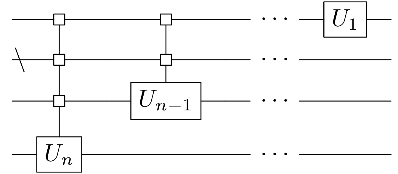
Figure 1. QSP quantum circuit utilizing uniformly controlled gates.

One way to visualize the sequence of multiplexers used for state preparation is as a tree-shaped graph. Each level of the tree contains $2^{k}$ nodes, representing the operators that need to be multiplexed by the corresponding size $2^{k}$ multiplexer, as illustrated in Figure 2, where the dotted edge represents an open control and the solid edge represents a closed control. The initialization of a quantum register with $n$ qubits requires $n-1$ multiplexers with $n-1,n-2,\cdots,0$ controls. A $k$-controlled multiplexer produces a circuit with depth proportional to $2^{k}$, then the state preparation circuit has depth proportional to $\sum_{k=0}^{n-1}2^{k}=2^{n}$.

Figure 2. Representation of a set of multiplexers using an abstract tree (a) and the corresponding quantum circuit (b). Here, a lowercase letter represents a one qubit quantum operator.

4. Multiplexers Simplification

4.1. Optimization Method

The crucial aspect of our proposed method is the relationship between state separation and the presence of repetition patterns in the multiplexers. By leveraging these repetition patterns to identify state separability, the multiplexer simplification can produce quantum circuits with reduced depth and fewer CNOT gates.

Identifying a repeated set of operators in the target qubit of a quantum multiplexer when their size and number of occurrences are a power of two indicates the presence of unnecessary controls. For instance, if the operators of a multiplexer are equal in an interleaved manner in each branch, as shown in Figure 3, only the first and the last controls are necessary to determine the result of the multiplexing. Therefore, the original multiplexer can be replaced with a simplified version. This new simplified multiplexer has only two controls and its number of gates and depth is halved.

Figure 3. Representation of a set of multiplexers used to prepare a specific state, with repetitions observed in the final multiplexer.

By utilizing the properties of a tree-shaped graph, we obtain a simplification rule that derives from the analysis of the abstract tree (Araujo et al., 2021, 2023d) that represents the set of multiplexers. Let $d$ denote the distance between repeated operators in the multiplexer. The control unnecessary is always located $\log_{2}(d)+1$ levels above the height of the multiplexer with the repetition pattern. This rule applies to all repetition patterns within the multiplexer. For example, the last multiplexer in Figure 3 exhibits repetitions in each of the two main branches for $d=2$. Consequently, controls two levels above the bottom level of the tree are eliminated, as shown in Figure 4.

Figure 4. Quantum circuit for QSP derived from the reduction applied to the tree in Fig. 3. Out of the eight single-qubit multi-controlled quantum gates (each with three controls), the algorithm eliminated four gates and reduced the controls from three to two for the remaining four gates.

The function implementing the proposed simplification approach is the Simplify function, as shown in Algorithm 1. The loop in line 2 traverses the abstract tree (represented as an array where each represents the operators applied on the target qubits of the multiplexer). The loop in lines 5-6 intends to add the position of the multiplexer controls to the set $c$. So, for each multiplexer, we call a search routine in line 8 that identifies repetitions in the array and returns the unnecessary controls and a copy of the array, marking the repeated operators as null. Finally, we remove the unnecessary controls and the marked operators, creating a new set of controls and a new array (in the loops in lines 10 and 15, respectively) representing the simplified multiplexer.

In the RepetitionSearch function, shown in Algorithm 2, the positions of the multiplexer that indices are a power of two are traveled by the loop in line 3 to find an operator identical to the first one. If a repeated angle is found, a copy of the array is done in line 6, and we calculate in the next line the number of repetitions for a possible pattern based on the distance between the two operators and the size of the multiplexer. Notice that each one has a length equal to 2d. In the next step, each possible repetition is verified in the loop in line 9 to confirm its validity. We call the verification function for each of them, which returns a boolean as true if the pattern is confirmed and marks the copy of the array as described previously. If the repetitions are invalid, we restore the array to the original format in line 14 and stop the search for this value of $d$. If all the repetitions for this pattern are confirmed, we have disentanglement, and the position of the unnecessary control is calculated in line 19 using the previous rule.

The RepetitionVerify function, shown in Algorithm 3, verifies if one repetition is valid by comparing each pair of operators with a distance $d$ between them. If all of these pairs are identical, the repetition for this pattern is consistent. Operators marked for removal are flagged as null without changing the array size.

In the example in Figure 3, we conclude that the repetition search is successful. When searching for repetitions at the last level of the tree, we note that for a distance $d=2$ from the first operator, the multiplexer operators start to repeat. Since $d$ is a power of 2, the multiplexer simplification is possible. The repetition patterns ”h-i-h-i” and ”j-k-j-k” with a size of $2d=4$ appear in the multiplexer list of size 8. We traverse both occurrences to verify if all operators at a distance of 2 are identical, marking all repeated operators to the right. If all occurrences are confirmed, we establish the separability. For $d=2$, the control at position $4-\log_{2}(d)-1=2$ is eliminated. So, we create a new multiplexer containing only the unmarked operators and the controls not eliminated.

The total cost of the multiplexer simplification is linearithmic in terms of the size of the multiplexer. In Algorithm 1, we make a copy of the array in line 4, which has a linear cost relative to the array size. The initialization of a set of control qubits indexes has a cost logarithmic, given that the number of controls of a multiplexer with size $N$ is equal to $\log_{2}{N}$. The loop in line 10 traverses this set and has a logarithmic cost too. In turn, the removal of marked operators has a linear cost. So, the total cost in the worst case to the simplification of one multiplexer is given by $O(2N+2\log_{2}{N}+C_{Search})$, where $C_{Search}$ is the cost of Algorithm 2. The call to the function in Algorithm 2 is the main contribution to the total time complexity, as explained below.

In Algorithm 2, we traveled the positions of the array whose index is a power of two. So, the operations at the interior of the while loop in line 3 are executed $O(\log_{2}{N})$ times. In the interior of the loop, the cost in the worst case is given by $O(N+\frac{N}{2d}\cdot C_{Verif})$, where $C_{Verif}$ is the cost of the Algorithm 3. This conclusion is valid because we copy the array in line 6, and the instructions in the interior of the loop in line 9 (the call to the function in Algorithm 3) are repeated according to the number of repetitions. As $C_{Verif}$ is in $O(d)$, the total cost of this algorithm in the worst case is $O(N\log_{2}{N})$. Therefore, we conclude that the cost of this approach to multiplexer simplification is linearithmic.

1

Data: $\textbf{muxes}.$

Result: controls_tree, muxes_tree.

2 Create two empty lists, $muxes\_tree$ and $controls\_tree$;

3 for $i\leftarrow 0$ to $\text{lenght}(muxes)$ do

4       $c\leftarrow\{\}$; $nc\leftarrow\{\}$;

5       Make a copy of $muxes[i]$ (mux_copy);

6       for $j\leftarrow 0$ to $\log_{2}(\text{lenght}(muxes[i]))$ do

7             Add $j+1$ to $c$;

8      if $\text{lenght}(muxes[i])>1$ then

9             $nc,mux\_copy\leftarrow\text{{RepetitionSearch}}(muxes[i],i,\text{mux\_copy})$;

10            

11      $controls\leftarrow\{\}$;

12       for $x$ in $c$ do

13             if $x$ not in $nc$ then

14                   Add $x$ to $controls$;

15                  

16            

17      Add $controls$ to $controls\_tree$;

18       Create an empty list $new\_mux$;

19       for $x$ in $mux\_copy$ do

20             if $x\neq\text{null}$ then

21                   Add $x$ to $new\_mux$;

22                  

23            

24      Add $new\_mux$ to $muxes\_tree$;

25return $controls\_tree$, $muxes\_tree$;

Algorithm 1 Simplify Function

Data: mux, n, mux_copy.

Result: nc , mux_copy.

1 $nc\leftarrow\{\}$;

2 $d\leftarrow 1$;

3 while $d\leq\text{lenght}(mux)/2$ do

4       $disentanglement\leftarrow\text{False}$;

5       if $mux[d]=mux[0]$ then

6             Make a copy of mux_copy (mux_org);

7             $repetitions\leftarrow\text{lenght}(mux)/(2d)$;

8             $p\leftarrow 0$;

9             while $repetitions>0$ do

10                   $repetitions\leftarrow repetitions-1$;

11                   $valid,mux\_copy\leftarrow\text{{RepetitionVerify}}(p,d,mux,mux\_copy)$;

12                   $p\leftarrow p+2d$;

13                   if not $valid$ then

14                         $mux\_copy\leftarrow mux\_org$;

15                         Break the while loop;

16                        

17                  if $repetitions=0$ then

18                         $disentanglement\leftarrow\text{True}$;

19                        

20                  

21            

22      if $disentanglement$ then

23             $removed\_control\leftarrow n-\log_{2}d$;

24             Add $removed\_control$ to $nc$;

25      $d\leftarrow 2\cdot d$;

26      

return $nc$, $mux\_copy$;

Algorithm 2 RepetitionSearch Function

Data: a, d, mux, mux_copy.

Result: a boolean value, mux_copy.

1 $i\leftarrow 0$;

2 $b\leftarrow a+d$;

3 while $i<d$ do

4       if $\text{mux}[a]\neq\text{mux}[b]$ then

5             return False, mux_copy;

6            

7      $mux\_copy[b]\leftarrow\text{null}$;

8       $a\leftarrow a+1$;

9       $b\leftarrow b+1$;

10       $i\leftarrow i+1$;

11      

12return True, mux_copy;

Algorithm 3 RepetitionVerify Function

4.2. Experiments and Discussion

To evaluate the efficiency of our simplification method for disentangled states, we conducted two experiments. The first experiment compares the circuit depth and the time required to create and transpile the circuits. We compare our simplification method, combined with the state preparation method from Ref. (Bergholm et al., 2005), denoted as UCGE (an acronym for the union of Uniformly Controlled One-Qubit Gates with Entanglement), with other state preparation approaches. In this experiment, we prepare a set of random real-valued disentangled states with varying numbers of qubits. Each state consists of two disentangled components, and the circuit depth is determined by its decomposition into CNOT and single-qubit gates. The results are presented in Figure 5.

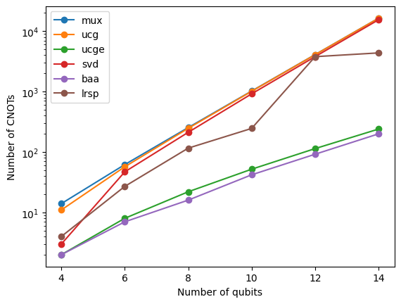
(a)

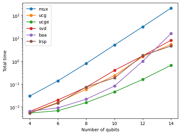
(b)

Figure 5. The number of CNOT gates in the circuit, along with the execution and transpilation times (in seconds), are compared for preparing a bipartite quantum state with varying numbers of qubits. The algorithms used for the comparison are: ‘mux’ (Shende et al., 2006), ‘ucg’ (Bergholm et al., 2005), ‘lrsp’ (Araujo et al., 2023b), ‘baa’ (Araujo et al., 2023b), ‘svd’ (Plesch and Brukner, 2011), and the proposed method ‘ucge’. The ‘mux’ algorithm is implemented in the Qiskit library (Javadi-Abhari et al., 2024), while the others are implemented in the Qclib library (Araujo et al., 2023a).

The second experiment fixes the number of qubits at twelve and varies the number of disentangled components within the state. The same QSP techniques are used for this experiment. The results are shown in Figure 6.

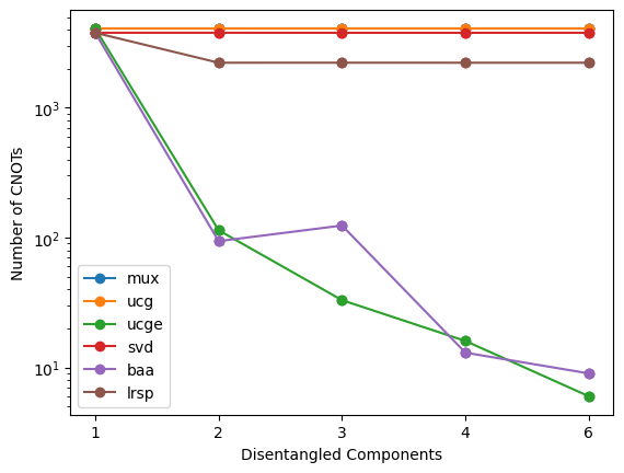
(a)

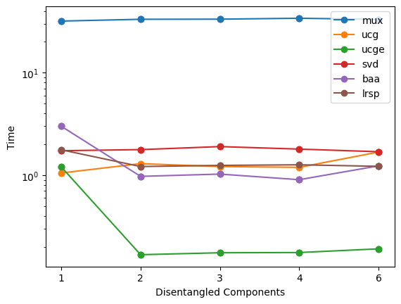
(b)

Figure 6. The number of CNOT gates in the circuit, along with the execution and transpilation times (in seconds), are compared to prepare an n-partite 12-qubit quantum state with equally sized partition blocks. The algorithms used for the comparison are: ‘mux’ (Shende et al., 2006), ‘ucg’ (Bergholm et al., 2005), ‘lrsp’ (Araujo et al., 2023b), ‘baa’ (Araujo et al., 2023b), ‘svd’ (Plesch and Brukner, 2011), and the proposed method ‘ucge’. The ‘mux’ algorithm is implemented in the Qiskit library (Javadi-Abhari et al., 2024), while the others are implemented in the Qclib library (Araujo et al., 2023a).

The reduction of the number of controls on the multiplexers explains why the QSP circuit has fewer CNOT gates when compared to previous state preparation approaches that do not detect separable states (Bergholm et al., 2005; Plesch and Brukner, 2011; Shende et al., 2006). Without separability detection, the CNOT gate count in the resulting circuit increases exponentially with the total number of qubits. Removing some controls significantly decreases the cost, as shown in Figure 5. Furthermore, as illustrated in Figure 6, the cost decreases as the number of disentangled components increases. In terms of exact state preparation, our results are highly competitive with the BAA method (Araujo et al., 2023b), which also employs separability detection for this purpose.

The crucial aspect that sets our approach apart from others is the efficient detection of separable states at a reduced computational cost. The proposed method demonstrates an advantage in the total time required to generate a state preparation circuit, including circuit generation and transpilation time. Transpilation into CNOT and unitary one-qubit operators is essential because quantum computers operate with a limited set of quantum gates. Our method’s shorter QSP time compared to strategies that do not detect disentanglement is due to replacing a multiplexer with smaller multiplexers that reduces the size of the transpiled circuit. As previously noted, the time for simplification search and application has a worst-case scenario of linearithmic complexity relative to the multiplexer size. Consequently, the impact of the search on the total QSP time is smaller than that of methods employing brute force search.

Another approach that also leverages state separability to reduce the QSP cost is the BAA strategy. This method prepares quantum states similarly to the Schmidt decomposition, utilizing a decomposition scheme for arbitrary full quantum gates (Plesch and Brukner, 2011). Employing a low-rank approximation reduces the number of CNOT gates, albeit with an arbitrary fidelity loss (Araujo et al., 2023b). Since the Schmidt approach deals with bipartite systems, the technique is recursively applied to multipartite systems, simplifying the two resulting partitions separately. This allows finding a set of partitions that maximizes the number of CNOT gates saved while maintaining bounded fidelity loss. The optimal configuration is identified through a search tree, leading to an exponential run-time concerning the number of qubits in the state to be approximated. Consequently, our method also demonstrates an advantage in total run-time compared to the BAA strategy. Figure 5 illustrates that the total time for BAA increases at a rate of $N/\log_{2}(N)$ compared to UCGE.

5. Conclusion

The quantum multiplexer simplification for state preparation reduces the number of CNOT gates required for QSP, reducing the time for state separation detection. This is accomplished by identifying repetitions in the abstract tree that describe the set of multiplexers implementing a quantum state. To demonstrate the utility of this approach, we compare our results with other techniques for encoding real-valued classical data into the amplitudes of a quantum state. The advantage of our method, which explores separability, is evident when preparing a separable state.

Future work could involve applying this optimization method to identify partial disentanglement using a search tree and low-rank approximation. Optimize other state preparation techniques and using it in various quantum encoding scenarios where multiplexers are needed, or separable states are common.

Data availability

The data and software generated during this study are available at https://github.com/qclib/qclib-papers and https://github.com/qclib/qclib (Araujo et al., 2023a).

Conflict of interests

All authors declare no conflicts of interest.

References

- (1)
- Araujo et al. (2023a) Israel F. Araujo, Ismael C. S. Araújo, Leon D. da Silva, Carsten Blank, and Adenilton J. da Silva. 2023a. Quantum computing library. https://github.com/qclib/qclib
- Araujo et al. (2023b) Israel F. Araujo, Carsten Blank, Ismael C. S. Araújo, and Adenilton J. da Silva. 2023b. Low-Rank Quantum State Preparation. Trans. Comp.-Aided Des. Integ. Cir. Sys. 43, 1 (July 2023), 161–170. https://doi.org/10.1109/TCAD.2023.3297972
- Araujo et al. (2023c) Israel F Araujo, Daniel K Park, Teresa B Ludermir, Wilson R Oliveira, Francesco Petruccione, and Adenilton J Da Silva. 2023c. Configurable sublinear circuits for quantum state preparation. Quantum Information Processing 22, 2 (2023), 123.
- Araujo et al. (2023d) Israel F. Araujo, Daniel K. Park, Teresa B. Ludermir, Wilson R. Oliveira, Francesco Petruccione, and Adenilton J. Da Silva. 2023d. Configurable sublinear circuits for quantum state preparation. Quantum Information Processing 22, 2 (2023), 123. https://doi.org/10.1007/s11128-023-03869-7
- Araujo et al. (2021) Israel F Araujo, Daniel K Park, Francesco Petruccione, and Adenilton J da Silva. 2021. A divide-and-conquer algorithm for quantum state preparation. Scientific reports 11, 1 (2021), 6329.
- Benioff (1982) Paul Benioff. 1982. Quantum mechanical Hamiltonian models of Turing machines. Journal of Statistical Physics 29 (1982), 515–546.
- Bergholm et al. (2005) Ville Bergholm, Juha J. Vartiainen, Mikko Möttönen, and Martti M. Salomaa. 2005. Quantum circuits with uniformly controlled one-qubit gates. Phys. Rev. A 71 (May 2005), 052330. Issue 5. https://doi.org/10.1103/PhysRevA.71.052330
- Feynman (1982) Richard P. Feynman. 1982. Simulating physics with computers. International Journal of Theoretical Physics 21, 6 (June 1982), 467–488. https://doi.org/10.1007/BF02650179
- Gleinig and Hoefler (2021) Niels Gleinig and Torsten Hoefler. 2021. An efficient algorithm for sparse quantum state preparation. In 2021 58th ACM/IEEE Design Automation Conference (DAC). IEEE, 433–438.
- Grover (2000) Lov K Grover. 2000. Synthesis of quantum superpositions by quantum computation. Physical review letters 85, 6 (2000), 1334.
- Gui et al. (2024) Kaiwen Gui, Alexander M Dalzell, Alessandro Achille, Martin Suchara, and Frederic T Chong. 2024. Spacetime-efficient low-depth quantum state preparation with applications. Quantum 8 (2024), 1257.
- Hughes et al. (1996) Richard J. Hughes, Daniel F. V. James, Emanuel H. Knill, Raymond Laflamme, and Albert G. Petschek. 1996. Decoherence Bounds on Quantum Computation with Trapped Ions. Phys. Rev. Lett. 77 (Oct. 1996), 3240–3243. Issue 15. https://doi.org/10.1103/PhysRevLett.77.3240
- Javadi-Abhari et al. (2024) Ali Javadi-Abhari, Matthew Treinish, Kevin Krsulich, Christopher J. Wood, Jake Lishman, Julien Gacon, Simon Martiel, Paul D. Nation, Lev S. Bishop, Andrew W. Cross, Blake R. Johnson, and Jay M. Gambetta. 2024. Quantum computing with Qiskit. https://doi.org/10.48550/arXiv.2405.08810 arXiv:2405.08810 [quant-ph]
- Long and Sun (2001) Gui-Lu Long and Yang Sun. 2001. Efficient scheme for initializing a quantum register with an arbitrary superposed state. Physical Review A 64, 1 (2001), 014303.
- Möttönen et al. (2005) Mikko Möttönen, JJ Vartiainen, Ville Bergholm, and Martti M Salomaa. 2005. Transformation of quantum states using uniformly controlled rotations. Quantum Information and Computation 5 (2005).
- Mozafari et al. (2022) Fereshte Mozafari, Giovanni De Micheli, and Yuxiang Yang. 2022. Efficient deterministic preparation of quantum states using decision diagrams. Physical Review A 106, 2 (2022), 022617.
- Nakaji et al. (2022) Kouhei Nakaji, Shumpei Uno, Yohichi Suzuki, Rudy Raymond, Tamiya Onodera, Tomoki Tanaka, Hiroyuki Tezuka, Naoki Mitsuda, and Naoki Yamamoto. 2022. Approximate amplitude encoding in shallow parameterized quantum circuits and its application to financial market indicators. Physical Review Research 4, 2 (2022), 023136.
- Nielsen and Chuang (2010) Michael A. Nielsen and Isaac L. Chuang. 2010. Quantum Computation and Quantum Information: 10th Anniversary Edition. Cambridge University Press, Cambridge, UK.
- Plesch and Brukner (2011) Martin Plesch and Časlav Brukner. 2011. Quantum-state preparation with universal gate decompositions. Phys. Rev. A 83 (March 2011), 032302. Issue 3. https://doi.org/10.1103/PhysRevA.83.032302
- Preskill (2018) John Preskill. 2018. Quantum computing in the NISQ era and beyond. Quantum 2 (2018), 79.
- Shende et al. (2006) V.V. Shende, S.S. Bullock, and I.L. Markov. 2006. Synthesis of quantum-logic circuits. IEEE Transactions on Computer-Aided Design of Integrated Circuits and Systems 25, 6 (2006), 1000–1010. https://doi.org/10.1109/TCAD.2005.855930
- Shor (1999) Peter W Shor. 1999. Polynomial-time algorithms for prime factorization and discrete logarithms on a quantum computer. SIAM review 41, 2 (1999), 303–332.
- Soklakov and Schack (2006) Andrei N. Soklakov and Rüdiger Schack. 2006. Efficient state preparation for a register of quantum bits. Physical Review A 73, 1 (jan 2006). https://doi.org/10.1103/physreva.73.012307
- Trugenberger (2001) C. A. Trugenberger. 2001. Probabilistic Quantum Memories. Physical Review Letters 87, 6 (jul 2001). https://doi.org/10.1103/physrevlett.87.067901
- Ventura and Martinez (1999) Dan Ventura and Tony Martinez. 1999. Initializing the amplitude distribution of a quantum state. Foundations of Physics Letters 12, 6 (1999), 547–559.
- Wootters and Zurek (1982) W. K. Wootters and W. H. Zurek. 1982. A single quantum cannot be cloned. Nature 299, 5886 (Oct. 1982), 802–803. https://doi.org/10.1038/299802a0
- Wu et al. (2021) Yulin Wu et al. 2021. Strong Quantum Computational Advantage Using a Superconducting Quantum Processor. Phys. Rev. Lett. 127 (Oct. 2021), 180501. Issue 18. https://doi.org/10.1103/PhysRevLett.127.180501