Observational constraints on $\alpha$-Starobinsky inflation

Abstract

In this work we revisit $\alpha$-Starobinsky inflation, also know as $E$-model, in the light of current CMB and LSS observations. The inflaton potential in the Einstein frame for this model contains a parameter $\alpha$ in the exponential, which alters the predictions for the scalar and tensor power spectra of Starobinsky inflation. We obtain these power spectra numerically without using slow-roll approximation and perform MCMC analysis to put constraints on parameters $M$ and $\alpha$ from Planck-2018, BICEP/Keck (BK18) and other LSS observations. We consider general reheating scenario by varying the number of e-foldings during inflation, $N_{pivot}$, along with the other parameters. We find $\log_{10}\alpha=0.0^{+1.6}_{-5.6}$, $\log_{10}M=-4.91^{+0.69}_{-2.7}$ and $N_{pivot}=53.2^{+3.9}_{-5}$ with $95\%$ C. L.. This implies that the present CMB and LSS observations are insufficient to constrain the parameter $\alpha$. We also find that there is no correlation between $N_{pivot}$ and $\alpha$.

I Introduction

Inflation Guth:1980zm is a theoretical framework in cosmology that proposes a brief and extremely rapid expansion of the early universe before big bang nucleosynthesis. It provides solution to some key puzzles of the big bang model such as the horizon problem, which is related to the uniformity of the cosmic microwave background radiation, and the flatness problem, which concerns the geometry of the universe. The driving force behind inflation is a hypothetical scalar field named as inflaton, whose potential energy dominates the energy density of the universe causing quasi-exponential expansion of the universe for a very short period of time. During this period the quantum fluctuations in the inflaton, which are coupled to the metric perturbations, give rise to the primordial density perturbations. The quantum fluctuations in the spacetime geometry during inflation are responsible for the primordial gravitational waves (tensor perturbations). These primordial perturbations generated during inflation provide seeds for cosmic microwave background anisotropy and structures in the universe. Observations of CMB anisotropy and polarization by COBE Smoot:1992td , WMAP Komatsu:2010fb , Planck Ade:2015lrj ; Planck:2018jri , and BICEP/Keck array offer robust experimental support for the predictions of inflation, i.e. adiabatic, nearly scale invariant and Gaussian perturbations. Since its inception, several models of inflation based on particle physics and string theory have been explored Martin:2013tda ; Martin:2024qnn . The most popular models of inflation, where inflaton has quadratic or quartic potentials, have been ruled out by Planck observations Planck:2018jri .

One of the well suited model of inflation from recent Planck and BICEP/Keck array observations is Starobinsky inflation Starobinsky:1980te ; Starobinsky:1983zz where inflation is achieved by $\frac{1}{M^{2}}R^{2}$ interaction, R being the Ricci scalar , in the Einstein Hilbert action without additional scalar field. In the Einstein frame the $R^{2}$ term gives rise to plateau potential of the inflaton, named as scalaron in this case. Starobinsky inflation is of great importance in the light of recent observations as it predicts a scalar tilt value of Mukhanov:1981xt $n_{s}\simeq 0.965$ and a smaller value of tensor-to-scalar ratio $r\simeq 0.003$. Besides this, it also incorporates a graceful exit to the radiation dominated epoch via reheating Vilenkin:1985md ; Mijic:1986iv ; Ford:1986sy , where the standard model particles were produced by the oscillatory decay of scalaron.

Another interesting feature of Starobinsky inflation is that the scalaron potential in the Einstein frame can be easily realized in the framework of no-scale supergravity Ellis:2013xoa with noncompact $SU(2,1)/SU(2)\times U(1)$ symmetry. In this case we have a modulus field that can be fixed by the other dynamics Ellis:2013nxa , and the inflaton field is a part of chiral superfield with a minimal Wess-Zumino superpotential. No-scale supergravity Cremmer:1983bf ; Ellis:1983sf ; Lahanas:1986uc , where the supersymmetry breaking scale is undetermined in a first approximation and the energy scale of the effective potential can be much smaller than the Planck scale, provides a framework to connect inflation to a viable quantum theory of gravity at high scales and the standard model of particle physics at lower scale. Attempts have been made to incorporate standard model of particle physics in no-scale supergravity models of inflation Ellis:2013nka ; Ellis:2015kqa ; Ellis:2016ipm ; Ellis:2017jcp . In Ellis:2013nxa ; Ellis:2018zya various possible examples in no-scale supergravity framework, which can reproduce the effective potential of the Starobinsky model and other related models, have been explored.

In this work we consider a variant of Starobinsky model known as $\alpha-$Starobinsky model of inflation Ellis:2013nxa , where the Einstein frame potential of the scalaron is modified by a parameter $\alpha$ in the exponential. This potential is obtained by generalizing the coefficient of the logarithm of the volume modulus field in the Kähler potenial in $SU(2,1)/SU(2)\times U(1)$ no-scale supergravity framework Ellis:1983ei ; Ellis:1984bm with a suitable choice of the superpotential having both the volume modulus field and the chiral superfield; the inflaton being the scalar part of the chiral superfield. Similar potentials can also be obtained in supergravity models where the inflaton is a part of the vector multiplet rather than the chiral multiplet Ferrara:2013rsa ; Kallosh:2013yoa . In this case the $\alpha-$Starobinsky model belongs to a class of superconformal inflationary models known as $\alpha-$attractors. The parameter $\alpha$ is crucial as it is connected to various physical aspects, such as the geometry of the k$\ddot{a}$hler manifold, hyperbolic geometry Carrasco:2015rva ; Kallosh:2015zsa ; Carrasco:2015uma , the behavior of the boundary of moduli space Kallosh:2014rga , modified gravity Odintsov:2016vzz , maximal supersymmetry Kallosh:2017ced , and string theory Scalisi:2018eaz ; Kallosh:2017wku . In Alho:2017opd $\alpha$-attractor models have been studied in the dynamical system framework to find inflationary attractor solutions in the light of observational viability of these models. A two-field inflation model where both the fields have $\alpha$-attractor potentials is studied in Rodrigues:2020fle . The $E$-model potential in brane inflation along with its various observational aspects has been studied in Sabir:2019wel . The primordial black hole formation in $\alpha$-attractor inflation models has been studied is Dalianis:2018frf ,Mahbub:2019uhl . The predictions for tensor-to-scalar ratio $r$ are modified in the $\alpha$-Starobinsky model by a factor of $\alpha$ Ellis:2013nxa ; Kallosh:2013yoa . To obtain constraints on $\alpha$, this model was analyzed with Planck-2015 observations in Planck:2015sxf , where the power spectra was calculated using public code ASPIC Martin:2013tda based on HFF’s $\epsilon_{i}$. By choosing a flat prior over [0,4] for $\log_{10}(\alpha^{2})$ it was found that $\log_{10}(\alpha^{2})<1.7(2.0)$ for E model and $\log_{10}(\alpha^{2})<2.3(2.5)$ at $95\%$ CL for T model of $\alpha$ attractors. Further, the Planck 2018 results have also placed an upper limit on the parameter $\alpha$ Planck:2018jri , $\log_{10}\alpha<1.3$ $(\alpha<19)$ for the E-model and $\log_{10}\alpha<1.0$ $(\alpha<10)$ for the T-model at $95\%$ CL by choosing the parameter range $-2<\log_{10}\alpha<4$. The constraints on $\alpha$ from Planck-2018 observations for few choices of e-folding along with various phenomenological aspects of this model were studied in Ellis:2020xmk , and it was found that the data was insufficient to constrain $\alpha$. However, an upper limit on $\alpha$ ($\alpha\leq 46(88)$ for e-folds $N=50(60)$) was obtained from the Planck upper limit on $r$ in Ueno:2016dim . In Ellis:2021kad the joint constraints on $n_{s}-r$ from Planck-2018 and BICEP/Keck observations were used to put constraints on the parameter $\alpha$ and the bounds on reheating temperature were used to put constraints on the e-folds $N$. Both these analysis were based on slow-roll approximation. Reheating constraints on $\alpha$-attractor models were also studied in Ueno:2016dim and it was found that the parameter $\alpha$ is roughly constrained as $\alpha\geq 0.01$ along a broad resonance preheating scenario. By assuming a two-phase reheating with a preheating for specific duration, constraint on $\alpha$ has been obtained in ElBourakadi:2022lqf and it is shown that small values of $\alpha$ give good results on $r$. The constraint on parameter $\alpha$ has also been obtained in Sarkar:2021ird by solving the cosmological perturbation equations in $k$-space.

Here, we analyze $\alpha$-Starobinsky inflation model in the light of Planck-2018, BICEP/Keck (BK18) and BAO observations to obtain constraints on parameter $\alpha$. To obtain the power spectra of primordial perturbations we use ModeChord, an updated version of ModeCode Mortonson:2010er , which solves the background and perturbation equations for inflaton numerically without the usual slow-roll approximation. ModeCode is coupled with CAMB Lewis:1999bs , which computes the angular power spectra for CMB anisotropy and polarization. The theoretical angular power spectra obtained with CAMB are used to compute constraints on inflationary parameters from CMB observations with the help of CosmoMC Lewis:2002ah . CosmoMC performs the Markov Chain Monte Carlo (MCMC) analysis, which is a statistical technique used to sample probability distributions of model parameters. By using ModeCode one can directly constrain the parameters of inflaton potential and $N_{pivot}$ (the number of e-foldings between horizon exit of the CMB pivot mode and the end of inflation) from CMB observations. To find the best-fit parameters of the $\alpha$-Starobinsky model, we vary $log_{10}\alpha$ between $-8.0$ to $4.0$ along with $M$ and $N_{pivot}$.

The format of this paper is as follows: A brief discussion of $\alpha$ - Starobinsky model is given in Sec.II. In section III, we obtain the background equations for Hubble parameter and inflaton in terms of e-foldings $N$. We also find perturbation equations for Mukhanov-Sasaki variable and tensor mode in terms of $N$. These equations are used in ModeCode. The details of MCMC analysis performed using CosmoMC along with observational constraints are described in section IV. In Section V, we provide our conclusions and a summary of our findings.

II $\alpha$-Starobinsky model(E-model)

The action for the Starobinsky inflation Starobinsky:1980te ; Starobinsky:1983zz contains $~{}R^{2}$ term due to quantum effects, and is given as

$$S_{J}=\frac{-M_{Pl}^{2}}{2}\int\sqrt{-g}(R+\mu R^{2})d^{4}x.$$ (1)

Here $\mu=\frac{1}{6M^{2}}$, $M$ is a parameter having a mass dimension of one and $M<<M_{Pl}$. $M_{Pl}$ is the reduced Planck mass ( $M_{Pl}^{2}=(8\pi G)^{-1}$) and $g$ is the determinant of the metric $g_{\mu\nu}$. After this point, we will work in units where $M_{Pl}=1$. After Weyl transformation $\tilde{g}_{\mu\nu}=(1+2\mu\phi)g_{\mu\nu}(x)$ and using the field redefinition $\chi\equiv\sqrt{\frac{3}{2}}\ln(1+\frac{\phi}{3M^{2}})$, the action Eq. (1) gets transformed to an Einstein Hilbert form:

$$S_{E}=\frac{1}{2}\int d^{4}x\sqrt{-\tilde{g}}\left(-\tilde{R}+\partial_{\mu}{\chi}\partial^{\mu}{\chi}+\frac{3}{2}M^{2}(1-e^{-\sqrt{\frac{2}{3}}\chi})^{2}\right).$$ (2)

It is evident from the above equation that the inflaton potential for Starobinsky inflation is given by:

$$V(\chi)=\frac{3}{4}M^{2}(1-e^{-\sqrt{\frac{2}{3}}\chi})^{2}$$ (3)

This model’s predictions for $n_{s}$ and r can be expressed as a function of the number of e-foldings $N_{e}$. In the limit of large $N_{e}$, one discovers

$$n_{s}=1-\frac{2}{N_{e}}$$ (4)

$$r=\frac{12}{N_{e}^{2}}$$ (5)

It is shown in Ellis:2013xoa that in the framework of no-scale supergravity with noncompact $SU(2,1)/SU(2)\times U(1)$ symmetry, one can obtain the inflaton potential (3), which can be generalized with the introduction of a new parameter $\alpha$ Ellis:2013nxa . This generalization is based on the Kähler potential Ellis:1983ei ; Ellis:1984bm

$$K=-3\alpha\ln\left(T+T^{\dagger}-\frac{\phi\phi^{\dagger}}{2}\right)$$ (6)

Here the field $T$ corresponds to a generic compactification volume modulus and $\phi$ is a part of generic chiral mater field. The parameter $\alpha$ is known as Kähler curvature parameter as it is inversely related to the curvature of the Kähler manifold ($R=\frac{2}{3\alpha}$). In Ellis:2013xoa the Wess-Zumino superpotential $W=M\left(\frac{\phi^{2}}{2}-\frac{\phi^{3}}{3\sqrt{3}}\right)$ was used to obtain the Starobinsky potential (3) in Einstein frame, along with the Kähler potential (6) for $\alpha=1$ yields

$$V(\phi)=3M^{2}\left(\frac{\phi}{\phi+\sqrt{3}}\right)^{2},$$ (7)

which with field redefinition $\phi=\sqrt{3}\tanh\left(\frac{\chi}{\sqrt{6}}\right)$ gives the Starobinsky potential (3).

For $\alpha\neq 1$ the field redefinition can be generalized as Ellis:2019bmm

$$\phi=\sqrt{3}\tanh\left(\frac{\chi}{\sqrt{6\alpha}}\right).$$ (8)

This, on substitution in (7), yields the potential for $\alpha$-Starobinsky inflation as

$$V(\chi)=\frac{3}{4}M^{2}(1-e^{-\sqrt{\frac{2}{3\alpha}}\chi})^{2}.$$ (9)

For any value of $\alpha$ the potential (9) can also be generated by considering the superpotential Ellis:2019bmm

$$W=\sqrt{\alpha}f(\phi)\left(2T-\frac{\phi^{2}}{3}\right)^{\frac{3}{2}(\alpha-\sqrt{\alpha})}.$$ (10)

To determine the function $f(\phi)$, $\phi$ and $T$ are considered to be real along with $\langle T\rangle=\frac{1}{2}$; and the potential obtained from the superpotential (10) is equated to (7). The superpotential (10) can be successfully combined with the dark energy and supersymmetry breaking Ellis:2019bmm .

The potential (9) can also be derived from supergravity models where the inflaton belongs to the vector superfield Ferrara:2013rsa ; Kallosh:2013yoa , and it belongs to a class of attractor models of inflation known as $\alpha$ - attractors. This potential, for $\alpha\leq{\cal O}(1)$ and large $N$, leads to a general prediction for inflationary observables Ellis:2013nxa ; Kallosh:2013yoa ,

$$n_{s}=1-\frac{2}{N_{e}},$$ (11)

$$r=\frac{12\alpha}{N_{e}^{2}}.$$ (12)

For $\alpha=1$, the potential (9)  corresponds to the Starobinsky-Whitt potential (3). On the other hand, for $\sqrt{\frac{2}{3\alpha}}<<1,$ this potential is quadratic.

$$V(\chi)=\frac{3}{4}M^{2}(1-e^{-\sqrt{\frac{2}{3\alpha}}\chi})^{2}=\frac{m^{2}}{2}\phi^{2},$$ (13)

where $m^{2}=\frac{M^{2}}{2}$. The $\alpha$ - Starobinsky potential (9) for different value of $\alpha$ is plotted in Fig. 1. It is evident from the Fig. that smaller the values of $\alpha$, narrower the potential minima. The potential has a wall for tiny negative $\chi$ and has an inflationary plateau at large positive $\chi$. It can be seen from the figure that increasing the value of curvature parameter $\alpha$ stretches the Starobinsky potential horizontally, which reduces the flatness of the plateau at any fixed value of $\chi$.

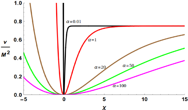
Figure 1: The variation of potential (9) with $\alpha=0.01,1,20,50,100$. The red line corresponds to the original Starobinsky inflationary potential with $\alpha=1$. The values of potential and field being in $M_{Pl}=1$ units.

III Inflationary dynamics and power spectra

As mentioned earlier, we use ModeCode to obtain the power spectra of scalar and tensor perturbations generated during inflation. ModeCode solves both the background and perturbation equations in terms of e-folds ($N$) as an independent variable numerically without slow-roll approximation. In this section we obtain the necessary equations describing the background dynamics during inflation and the perturbation equations in terms of e-folds. The evolution of the Hubble parameter during inflation is governed by the Friedmann equations:

$$H^{2} = \frac{1}{3}\left[\frac{1}{2}\dot{\chi^{2}}+V(\chi)\right].$$ (14)

$$\dot{H} = -\frac{1}{2}\dot{\chi^{2}},$$ (15)

where $V(\chi)$ is the potential (9) for the inflaton $\chi$ in the Einstein frame. The dynamics of the scalar field $\chi$ is governed by its equation of motion, which is the Klein-Gordon equation in spacetime:

$$\ddot{\chi}+3H\dot{\chi}+\frac{dV(\chi)}{d\chi}=0.$$ (16)

Here, the overdot denotes derivative with respect to cosmic time. As we use the number of e-folding, $N=\ln a$ as an independent variable to solve the equations numerically, we can rewrite the Friedmann equations (14) and (15) and the equation of motion of inflaton (16) in terms of $N$ as

$$H^{2} = \frac{\frac{1}{3}V(\chi)}{1-\frac{1}{6}\chi^{\prime 2}},$$ (17)

$$H^{\prime} = -\frac{1}{2}H\chi^{\prime 2},$$ (18)

and

$$\chi^{\prime\prime}+\left(\frac{H^{\prime}}{H}+3\right)\chi^{\prime}+\frac{1}{H^{2}}\frac{dV(\chi)}{d\chi}=0,$$ (19)

where prime denotes the differentiation with respect to $N$. The numerical solution of these equations provides various background quantities that are used in perturbations equations. We describe the scalar perturbation generated during inflation by the gauge invariant Mukhanov-Sasaki variable $u_{k}$ Mukhanov:1988jd ; Sasaki:1986hm , which is related to the curvature perturbations $\mathcal{R}$ as $u_{k}=-z\cal{R}$, where $z=\frac{1}{H}\frac{d\chi}{d\tau}$ and $\tau$ denotes the conformal time. The quantity $z$ can be determined from background equations Eqs. (18) and (19). The Fourier modes

$$u_{k}(\tau)=\int d^{3}xe^{-ik.x}u(\tau,x)$$ (20)

satisfies the Mukhanov-Sasaki equation

$$\frac{d^{2}u_{k}}{d\tau^{2}}+\left(k^{2}-\frac{1}{z}\frac{d^{2}z}{d\tau^{2}}\right)u_{k}=0,$$ (21)

The primordial power spectrum of scalar perturbations is given in terms of the two point correlation function of comoving curvature and its relation with Mukhanov-Sasaki variable $u_{k}$ is given by Eq. (22)and Eq. (23) respectively:

$$\mathcal{P_{\mathcal{R}}}=\frac{k^{3}}{2\pi^{2}}\langle\mathcal{R}_{k}\mathcal{R}_{k^{\prime}}^{*}\rangle\delta^{3}(k-k^{\prime}),$$ (22)

which can be expressed in terms of Mukhanov-Sasaki variable $u_{k}$ as

$$\mathcal{P_{\mathcal{R}}}(k)=\frac{k^{3}}{2\pi^{2}}\bigg{|}\frac{u_{k}}{z}\bigg{|}^{2}.$$ (23)

Similarly, for tensor perturbations, the mode equation and the primordial tensor power spectrum is given by following equations:

$$\frac{d^{2}v_{k}}{d\tau^{2}}+\left(k^{2}-\frac{1}{a}\frac{d^{2}a}{d\tau^{2}}\right)v_{k}=0,$$ (24)

$$\mathcal{P}_{t}(k)=\frac{4k^{3}}{\pi^{2}}\bigg{|}\frac{v_{k}}{a}\bigg{|}^{2}.$$ (25)

To obtain the scalar and tensor power spectra, the mode equations (21) and (24) are solved numerically along with background equations (18) and (19). For this we can rewrite these equations in terms of e-foldings $N=\ln a$ as

$$u_{k}^{\prime\prime}+\left(\frac{H^{\prime}}{H}+1\right)u_{k}^{\prime}+\Biggl{\{}\frac{k^{2}}{a^{2}H^{2}}-\left[2-4\frac{H^{\prime}}{H}\frac{\chi^{\prime\prime}}{\chi^{\prime}}-2\left(\frac{H^{\prime}}{H}\right)^{2}-5\frac{H^{\prime}}{H}-\frac{1}{H^{2}}\frac{d^{2}V}{d\chi^{2}}\right]\Biggr{\}}u_{k}=0,$$ (26)

$$v_{k}^{\prime\prime}+\left(\frac{H^{\prime}}{H}+1\right)v_{k}^{\prime}+\left[\frac{k^{2}}{a^{2}H^{2}}-\left(\frac{H^{\prime}}{H}+2\right)\right]v_{k}=0.$$ (27)

In this approach the scalar spectral index $n_{s}$ and the tensor spectral index $n_{t}$ are not the parameter of the power spectra, and hence they are determined from the power spectra obtained numerically using their definitions Bassett:2005xm :

$$n_{s} = 1+\frac{d\ln\mathcal{P_{\mathcal{R}}}}{d\ln k},$$ (28)

$$n_{t} = \frac{d\ln\mathcal{P}_{t}}{d\ln k},$$ (29)

Similarly, the tensor-to-scalar ratio $r$, defined by Bassett:2005xm

$$r=\frac{\mathcal{P}_{t}}{\mathcal{P_{\mathcal{R}}}},$$ (30)

is also a derived parameter and is obtained from the numerical solution of the power spectra. Both $n_{s}$ and $r$ are determined at the pivot scale $k=0.05$Mpc^-1. By obtaining the power spectra numerically the parameters of the inflaton potential (9), $M$ and $\alpha$ can be directly constrained from the CMB and LSS observations.

IV OBSERVATIONAL CONSTRAINTS

The background and perturbations equations, described in the previous section, are solved by ModeCode Mortonson:2010er numerically without using slow roll approximation. Thus, slow-roll violating effects, which can be significant for confronting models with precision data, are automatically captured. We modify ModeChord, un updated version of ModeCode, to compute the scalar and tensor power spectra for $\alpha$-Starobinsky inflation in the Einstein frame. Inflationary models are described in ModeCode using an array of parameters for the potential. We incorporate the parameters $M$ and $\alpha$ of the potential (9) in this array. Without depending on the slow roll approximation, we consider the general reheating scenario, where the parameter $N_{pivot}$ representing the number of e-foldings from the end of inflation to the time when length scales corresponding to the Fourier mode $k_{pivot}$ leave the horizon during inflation, is also varied along with other potential parameters. The numerically computed primordial power spectra with ModeChord can be used in CAMB Lewis:1999bs , which solves Boltzmann equation and computes the two-point correlation function for CMB temperature anisotropy and polarization for a given set of cosmological parameters. CosmoMC uses these theoretical angular power spectra to put constraints on the parameters of the inflaton potential, $N_{pivot}$, and the other parameters of the $\lambda$CDM model from various CMB and large-scale structure observations. We use Planck-2018, BICEP (BK18) BICEP:2021xfz , BAO and Pantheon data to determine the constraints on the parameters $M$ and $\alpha$ of inflaton potential (9) and $N_{pivot}$ . We have used flat priors for these parameters, which are given in Table 1. To cover a wide range, we sample $M$ and $\alpha$ on a logarithmic scale. We also vary the parameters of the $\Lambda$CDM model with their priors provided in Planck:2018vyg . To ensure MCMC convergence, we analyze four chains using the Gelman and Rubin $R-1$ statistics, which evaluates the “variance of the mean” against the “mean of the chain variance.”

Parameter	Prior range
$\mathbf{N_{\text{pivot}}}$	[20, 90]
$\mathbf{\log_{10}M}$	[-10.0, -1.0]
$\mathbf{\log_{10}\alpha}$	[-8.0, 4.0]

Table 1: Priors on $N_{pivot}$ and model parameters.

Table 2 shows the constraints obtained from MCMC analysis for parameters of potential (9), the e-foldings $N_{pivot}$ and the derived parameters, $r$ and $n_{s}$.

Parameter	68% limits	95% limits	99% limits
$N_{\text{pivot}}$	$53.2^{+2.9}_{-1.5}$	$53.2^{+3.9}_{-5.0}$	$53.2^{+4.3}_{-7.2}$
$\log_{10}M$	$-4.91^{+0.54}_{-0.043}$	$-4.91^{+0.69}_{-2.7}$	$-4.91^{+0.72}_{-3.3}$
$\log_{10}\alpha$	$0.022^{+1.2}_{+0.023}$	$0.0^{+1.6}_{-5.6}$	$0.0^{+1.4}_{-7.3}$
$n_{s}$	$0.9644^{+0.0027}_{-0.0017}$	$0.9644^{+0.0038}_{-0.0044}$	$0.9644^{+0.0045}_{-0.0064}$
$r$	$0.0121^{+0.0073}_{-0.012}$	$0.012^{+0.020}_{-0.016}$	$0.012^{+0.028}_{-0.019}$

Table 2: Constraints on parameters of potential, $r$ and $n_{s}$ using Planck-2018, BICEP/Keck (BK18) and BAO observations.

It can be seen from the Table 2 that the mean value of $\alpha$ along with $95\%\,C.L.$ is

$$\log_{10}\alpha=0.0^{+1.6}_{-5.6}.$$ (31)

As the limits are larger than the mean value, $\alpha=1$ is consistent with the Planck-2018 and BICEP/Keck (BK18) observations. So the present data is not sufficient to constrain the value of $\alpha$; a similar result was obtained in Ellis:2020xmk . The $95\%$ upper limit obtained on $\alpha$ in our analysis, i.e. $\log_{10}\alpha\leq 1.6$ is slightly larger than that obtained by Planck-2018 Planck:2018jri . This difference arises as we have varied $M$ and $N_{pivot}$ along with $\alpha$. However, the upper limit on $\alpha$ obtained in our analysis, i.e, $\alpha\leq 39.81$ with $95\%$ C.L., is smaller than the one obtained in Ellis:2021kad , and the lower limit, $\alpha\geq 2.51^{-6}$ with $95\%$ C.L., is also smaller than the lower limit obtained in Ueno:2016dim using a broad resonance preheating. The number of e-folding obtained for $\alpha$-Starobinsky model with $95\%\,C.L.$ is

$$N_{pivot}=53.2^{+3.9}_{-5.0},$$ (32)

which is sufficient to solve the horizon problem.

The best fit values of scalar spectral index $n_{s}$ and tensor-to-scalar ratio $r$ for $\alpha$-Starobinsky model, derived from the potential parameters, lie within the limits obtained by Planck-2018 and BICEP/Keck (BK18) observations as shown in Table 2. Fig.2 shows the marginalized probability distributions for various inflationary parameters, while Figs. 3 and 5 illustrate the marginalized joint $68\%$ and $95\%$ constraints on the potential parameters $\alpha$ and $M$, as well as the e-folds $N_{pivot}$. It can be seen from Fig. 2 that the most probable value of $\log_{10}\alpha$ is around $0.81$, however, it does not have any statistical significance as the limits are quite large compared to mean value. As depicted in Fig. 3 the potential parameters $\alpha$ and $M$ are strongly correlated. However, Fig.3(a) and Fig.5 show that there is no correlation between the e-folds $N_{pivot}$ and potential parameters $\alpha$ and $M$ respectively. The joint $68\%$ and $95\%$ C.L. constraints on scalar spectral index $n_{s}$ and tensor-to-scalar ratio $r$ are shown in Fig. 5. As these two parameters are derived parameters, the constraints on them are obtained from the constraints on potential parameters and $N_{pivot}$.

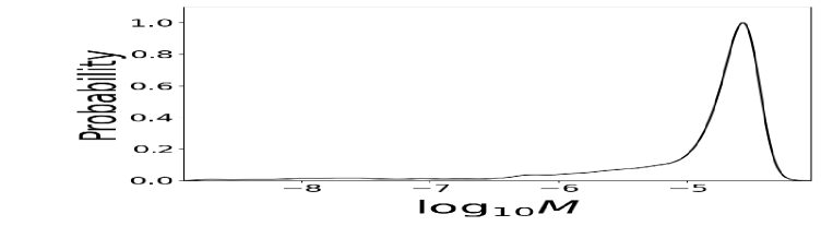
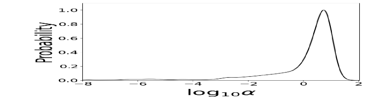
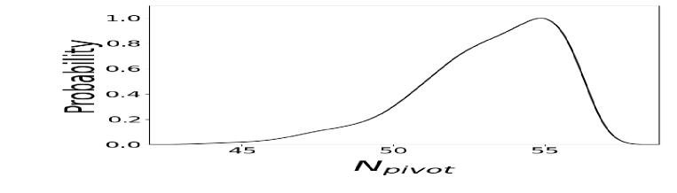
Figure 2: Marginalized probability constraints on the potential parameters and $N_{pivot}$ from Planck-2018, BICEP/Keck (BK18) and BAO data

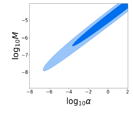
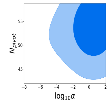
(a)

Figure 3: Marginalized joint two-dimensional $68\%$ C.L. and $95\%$ C.L. constraints on parameters of potential (a) and $N_{pivot}$ (b) using Planck-2018, BICEP/Keck (BK18) and BAO data

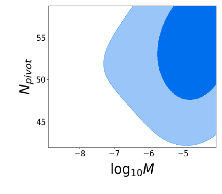
Figure 4: $1\sigma$ and $2\sigma$ confidence contours in the
potential parameter $\log_{10}M$ and $N_{pivot}$ parameter space

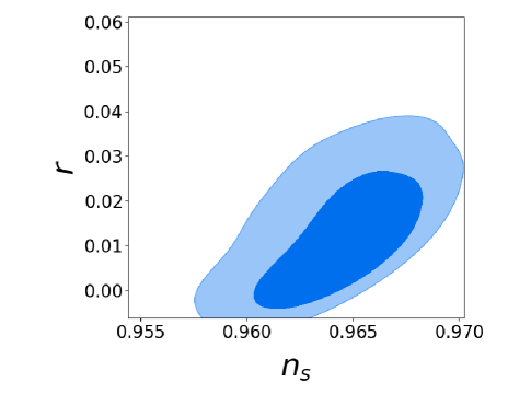
Figure 5: 1$\sigma$ and 2$\sigma$ confidence contours in the $n_{s}$-$r$ parameter space

V Conclusions

Starobinsky inflation Starobinsky:1980te ; Starobinsky:1983zz is one of the best suited model of inflation from the Planck-2018 Planck:2018jri and BICEP/Keck (BK18) BICEP:2021xfz observations as it predicts smaller value for tensor-to-scalar ratio $r$. The inflaton potential of this model in the Einstein frame can be derived from no-scale supergravity with an underlying noncompact $SU(2,1)/SU(2)\times U(1)$ symmetry Ellis:2013xoa , where the modulus field $T$ of the Kähler potential is fixed by other dynamics and inflaton field $\phi$ is a part of the chiral superfield with a minimum Wess-Zumino superpotential. By generalizing the coefficient of the logarithm of the volume modulus field in the Kähler potential that parameterizes $SU(2,1)/SU(2)\times U(1)$ coset Kähler manifold, and considering a superpotential having both the volume modulus field and inflaton field $\phi$, one can obtain a potential for inflaton that is similar to Starobinsky model with a parameter $\alpha$ in the exponential Ellis:2013nxa , known as $\alpha$-Starobinsky inflation. One can also obtain similar potential in supergravity models with inflaton as a part of vector multiplet rather than chiral multiplet Ferrara:2013rsa ; Kallosh:2013yoa , and the $\alpha$-Starobinsky model belongs to a class of superconformal inflationary models known as $E$-models of $\alpha$-attractors.

In this work we have used the inflation potential (9) to analyze $\alpha-$ attractor $E$-model, in the light of Planck-2018 and BICEP/Keck (BK18) BICEP:2021xfz CMB observations and other LSS observations. We have used ModeChord, an updated version of ModeCode Mortonson:2010er to numerically compute the power spectra of both scalar and tensor perturbations without slow-roll approximation. This helps us to constrain the number of e-foldings $N_{pivot}$ and the model parameter $\alpha$ and $M$ using CMB and LSS observations by MCMC analysis using CosmoMC Lewis:2002ah . To explore the parameter range we vary $log_{10}\alpha$ between $-8$ to $4$. In our analysis we find that $log_{10}\alpha=0.0^{+1.6}_{-5.6},\,\,\,95\%$ C.L. from Planck-2018, BICEP/Keck (BK18) and BAO data. The larger limits than the mean value on $\alpha$ indicates that the current observations are consistent with $\alpha=1$, which highlights the challenge in precisely determining $\alpha$ from current observational data, The $95\%$ upper limit on $\alpha$, $\log_{10}\alpha\leq 1.6$ or $\alpha\leq 39.81$, obtained in our analysis is slightly larger than the one obtained by Planck-2018 Planck:2018jri i.e. $\log_{10}\alpha\leq 1.3$, but, smaller than the one obtained by Ellis:2021kad , which is $\alpha\leq 46$. By considering general reheating scenario we find that the number of e-foldings from the end of inflation to the time when the length scales corresponding to $k_{pivot}$ leave the Hubble radius during inflation $N_{pivot}=53.2^{+3.9}_{-5.0}$ with $95\%$ C. L., which is sufficient to solve horizon problem. We also find that the potential parameters $M$ and $\alpha$ are strongly correlated, Fig. 3; and there is no correlation between these two parameters and $N_{pivot}$ as shown in Fig. 3(a) and Fig. 5.

The parameter $\alpha$ of the $\alpha$-Starobinsky model is inversely related to the curvature of the Kähler manifold. As the parameter $\alpha$ affects the amplitude of tensor perturbations, it will be possible with the future observations like CMB-S4 Abazajian:2019eic and LiteBIRD Hazumi:2019lys to obtain its precise value. The $\alpha$-Starobinsky inflation can be incorporated in a flipped $SU(5)\times U(1)$ GUT Ellis:2019jha ; Ellis:2019opr , where inflaton decay during reheating can produce cold dark matter and also can have implications for neutrinos masses and leptogenesis. The precise determination of the parameter $\alpha$ will help us in connecting the models of particle physics phenomenology with inflation in the framework of supergravity and string theory.

VI ACKNOWLEDGEMENTS

The authors would like to thank ISRO Department of Space Govt. of India to provide financial support via RESPOND programme Grant No. DS_2B-13012(2)/47/2018-Sec.II.

References

- (1) A. H. Guth, Phys. Rev. D23, 347 (1981).
- (2) G. F. Smoot, C. L. Bennett, A. Kogut, E. L. Wright, J. Aymon, N. W. Boggess, E. S. Cheng, G. De Amici et al., Astrophys. J. 396, L1-L5 (1992).
- (3) E. Komatsu et al. [ WMAP Collaboration ], Astrophys. J. Suppl. 192, 18 (2011). [arXiv:1001.4538 [astro-ph.CO]].
- (4) P. A. R. Ade et al. [Planck Collaboration], Astron. Astrophys. 594, A20 (2016) doi:10.1051/0004-6361/201525898 [arXiv:1502.02114 [astro-ph.CO]].
- (5) Y. Akrami et al. [Planck], Astron. Astrophys. 641, A10 (2020) doi:10.1051/0004-6361/201833887 [arXiv:1807.06211 [astro-ph.CO]].
- (6) J. Martin, C. Ringeval and V. Vennin, Phys. Dark Univ. 5-6, 75-235 (2014) doi:10.1016/j.dark.2014.01.003 [arXiv:1303.3787 [astro-ph.CO]].
- (7) J. Martin, C. Ringeval and V. Vennin, [arXiv:2404.10647 [astro-ph.CO]].
- (8) A. A. Starobinsky, Phys. Lett. B 91, 99-102 (1980) doi:10.1016/0370-2693(80)90670-X
- (9) A. A. Starobinsky, Sov. Astron. Lett. 9, 302 (1983)
- (10) V. F. Mukhanov and G. V. Chibisov, JETP Lett. 33, 532-535 (1981)
- (11) A. Vilenkin, Phys. Rev. D 32, 2511 (1985) doi:10.1103/PhysRevD.32.2511
- (12) M. B. Mijic, M. S. Morris and W. M. Suen, Phys. Rev. D 34, 2934 (1986) doi:10.1103/PhysRevD.34.2934
- (13) L. H. Ford, Phys. Rev. D 35, 2955 (1987) doi:10.1103/PhysRevD.35.2955
- (14) J. Ellis, D. V. Nanopoulos and K. A. Olive, Phys. Rev. Lett. 111, 111301 (2013) [erratum: Phys. Rev. Lett. 111, no.12, 129902 (2013)] doi:10.1103/PhysRevLett.111.111301 [arXiv:1305.1247 [hep-th]].
- (15) J. Ellis, D. V. Nanopoulos and K. A. Olive, JCAP 10, 009 (2013) doi:10.1088/1475-7516/2013/10/009 [arXiv:1307.3537 [hep-th]].
- (16) E. Cremmer, S. Ferrara, C. Kounnas and D. V. Nanopoulos, Phys. Lett. B 133, 61 (1983) doi:10.1016/0370-2693(83)90106-5
- (17) J. R. Ellis, A. B. Lahanas, D. V. Nanopoulos and K. Tamvakis, Phys. Lett. B 134, 429 (1984) doi:10.1016/0370-2693(84)91378-9
- (18) A. B. Lahanas and D. V. Nanopoulos, Phys. Rept. 145, 1 (1987) doi:10.1016/0370-1573(87)90034-2
- (19) J. Ellis, D. V. Nanopoulos and K. A. Olive, Phys. Rev. D 89, no.4, 043502 (2014) doi:10.1103/PhysRevD.89.043502 [arXiv:1310.4770 [hep-ph]].
- (20) J. Ellis, M. A. G. Garcia, D. V. Nanopoulos and K. A. Olive, JCAP 10, 003 (2015) doi:10.1088/1475-7516/2015/10/003 [arXiv:1503.08867 [hep-ph]].
- (21) J. Ellis, M. A. G. Garcia, N. Nagata, D. V. Nanopoulos and K. A. Olive, JCAP 11, 018 (2016) doi:10.1088/1475-7516/2016/11/018 [arXiv:1609.05849 [hep-ph]].
- (22) J. Ellis, M. A. G. Garcia, N. Nagata, D. V. Nanopoulos and K. A. Olive, JCAP 07, 006 (2017) doi:10.1088/1475-7516/2017/07/006 [arXiv:1704.07331 [hep-ph]].
- (23) J. Ellis, D. V. Nanopoulos, K. A. Olive and S. Verner, JHEP 03, 099 (2019) doi:10.1007/JHEP03(2019)099 [arXiv:1812.02192 [hep-th]].
- (24) J. R. Ellis, C. Kounnas and D. V. Nanopoulos, Nucl. Phys. B 241, 406-428 (1984) doi:10.1016/0550-3213(84)90054-3
- (25) J. R. Ellis, C. Kounnas and D. V. Nanopoulos, Nucl. Phys. B 247, 373-395 (1984) doi:10.1016/0550-3213(84)90555-8
- (26) S. Ferrara, R. Kallosh, A. Linde and M. Porrati, Phys. Rev. D 88, no.8, 085038 (2013) doi:10.1103/PhysRevD.88.085038 [arXiv:1307.7696 [hep-th]].
- (27) R. Kallosh, A. Linde and D. Roest, JHEP 11, 198 (2013) doi:10.1007/JHEP11(2013)198 [arXiv:1311.0472 [hep-th]].
- (28) J. J. M. Carrasco, R. Kallosh and A. Linde, Phys. Rev. D 92, no.6, 063519 (2015) doi:10.1103/PhysRevD.92.063519 [arXiv:1506.00936 [hep-th]].
- (29) R. Kallosh and A. Linde, Comptes Rendus Physique 16, 914-927 (2015) doi:10.1016/j.crhy.2015.07.004 [arXiv:1503.06785 [hep-th]].
- (30) J. J. M. Carrasco, R. Kallosh, A. Linde and D. Roest, Phys. Rev. D 92, no.4, 041301 (2015) doi:10.1103/PhysRevD.92.041301 [arXiv:1504.05557 [hep-th]].
- (31) R. Kallosh, A. Linde and D. Roest, JHEP 08, 052 (2014) doi:10.1007/JHEP08(2014)052 [arXiv:1405.3646 [hep-th]].
- (32) S. D. Odintsov and V. K. Oikonomou, Phys. Rev. D 94, no.12, 124026 (2016) doi:10.1103/PhysRevD.94.124026 [arXiv:1612.01126 [gr-qc]].
- (33) R. Kallosh, A. Linde, T. Wrase and Y. Yamada, JHEP 04, 144 (2017) doi:10.1007/JHEP04(2017)144 [arXiv:1704.04829 [hep-th]].
- (34) M. Scalisi and I. Valenzuela, JHEP 08, 160 (2019) doi:10.1007/JHEP08(2019)160 [arXiv:1812.07558 [hep-th]].
- (35) R. Kallosh, A. Linde, D. Roest, A. Westphal and Y. Yamada, JHEP 02, 117 (2018) doi:10.1007/JHEP02(2018)117 [arXiv:1707.05830 [hep-th]].
- (36) A. Alho and C. Uggla, Phys. Rev. D 95, no.8, 083517 (2017) doi:10.1103/PhysRevD.95.083517 [arXiv:1702.00306 [gr-qc]].
- (37) J. G. Rodrigues, S. Santos da Costa and J. S. Alcaniz, Phys. Lett. B 815, 136156 (2021) doi:10.1016/j.physletb.2021.136156 [arXiv:2007.10763 [astro-ph.CO]].
- (38) M. Sabir, W. Ahmed, Y. Gong and Y. Lu, Eur. Phys. J. C 80, no.1, 15 (2020) doi:10.1140/epjc/s10052-019-7589-3 [arXiv:1903.08435 [gr-qc]].
- (39) I. Dalianis, A. Kehagias and G. Tringas, JCAP 01, 037 (2019) doi:10.1088/1475-7516/2019/01/037 [arXiv:1805.09483 [astro-ph.CO]].
- (40) R. Mahbub, Phys. Rev. D 101, no.2, 023533 (2020) doi:10.1103/PhysRevD.101.023533 [arXiv:1910.10602 [astro-ph.CO]].
- (41) P. A. R. Ade et al. [Planck Collaboration], Astron. Astrophys. 594, A20 (2016) doi:10.1051/0004-6361/201525898 [arXiv:1502.02114 [astro-ph.CO]].
- (42) J. Ellis, D. V. Nanopoulos, K. A. Olive and S. Verner, JCAP 08, 037 (2020) doi:10.1088/1475-7516/2020/08/037 [arXiv:2004.00643 [hep-ph]].
- (43) Y. Ueno and K. Yamamoto, Phys. Rev. D 93, no.8, 083524 (2016) doi:10.1103/PhysRevD.93.083524 [arXiv:1602.07427 [astro-ph.CO]].
- (44) J. Ellis, M. A. G. Garcia, D. V. Nanopoulos, K. A. Olive and S. Verner, Phys. Rev. D 105, no.4, 043504 (2022) doi:10.1103/PhysRevD.105.043504 [arXiv:2112.04466 [hep-ph]].
- (45) K. El Bourakadi, Z. Sakhi and M. Bennai, Int. J. Mod. Phys. A 37, no.17, 2250117 (2022) doi:10.1142/S0217751X22501172 [arXiv:2209.09241 [gr-qc]].
- (46) A. Sarkar, C. Sarkar and B. Ghosh, JCAP 11, no.11, 029 (2021) doi:10.1088/1475-7516/2021/11/029 [arXiv:2106.02920 [gr-qc]].
- (47) M. J. Mortonson, H. V. Peiris and R. Easther, Phys. Rev. D 83, 043505 (2011) doi:10.1103/PhysRevD.83.043505 [arXiv:1007.4205 [astro-ph.CO]].
- (48) A. Lewis, A. Challinor and A. Lasenby, Astrophys. J. 538, 473-476 (2000) doi:10.1086/309179 [arXiv:astro-ph/9911177 [astro-ph]].
- (49) A. Lewis and S. Bridle, Phys. Rev. D 66, 103511 (2002) doi:10.1103/PhysRevD.66.103511 [arXiv:astro-ph/0205436 [astro-ph]].
- (50) S. Cecotti, Phys. Lett. B 190, 86-92 (1987) doi:10.1016/0370-2693(87)90844-6
- (51) J. Ellis, D. V. Nanopoulos, K. A. Olive and S. Verner, JCAP 09, 040 (2019) doi:10.1088/1475-7516/2019/09/040 [arXiv:1906.10176 [hep-th]].
- (52) V. F. Mukhanov, Sov. Phys. JETP 67, 1297-1302 (1988)
- (53) M. Sasaki, Prog. Theor. Phys. 76, 1036 (1986) doi:10.1143/PTP.76.1036
- (54) B. A. Bassett, S. Tsujikawa and D. Wands, Rev. Mod. Phys. 78, 537-589 (2006) doi:10.1103/RevModPhys.78.537 [arXiv:astro-ph/0507632 [astro-ph]].
- (55) P. A. R. Ade et al. [BICEP and Keck], Phys. Rev. Lett. 127, no.15, 151301 (2021) doi:10.1103/PhysRevLett.127.151301 [arXiv:2110.00483 [astro-ph.CO]].
- (56) N. Aghanim et al. [Planck], Astron. Astrophys. 641, A6 (2020) [erratum: Astron. Astrophys. 652, C4 (2021)] doi:10.1051/0004-6361/201833910 [arXiv:1807.06209 [astro-ph.CO]].
- (57) K. Abazajian, G. Addison, P. Adshead, Z. Ahmed, S. W. Allen, D. Alonso, M. Alvarez, A. Anderson, K. S. Arnold and C. Baccigalupi, et al. [arXiv:1907.04473 [astro-ph.IM]].
- (58) M. Hazumi, P. A. R. Ade, Y. Akiba, D. Alonso, K. Arnold, J. Aumont, C. Baccigalupi, D. Barron, S. Basak and S. Beckman, et al. J. Low Temp. Phys. 194, no.5-6, 443-452 (2019) doi:10.1007/s10909-019-02150-5
- (59) J. Ellis, M. A. G. Garcia, N. Nagata, D. V. Nanopoulos and K. A. Olive, Phys. Lett. B 797, 134864 (2019) doi:10.1016/j.physletb.2019.134864 [arXiv:1906.08483 [hep-ph]].
- (60) J. Ellis, M. A. G. Garcia, N. Nagata, D. V. Nanopoulos and K. A. Olive, JCAP 01, 035 (2020) doi:10.1088/1475-7516/2020/01/035 [arXiv:1910.11755 [hep-ph]].