Finite time quantum-classical correspondence in quantum chaotic systems

Abstract

Although the importance of the quantum-classical correspondence has been recognized in numerous studies of quantum chaos, whether it still holds for finite time dynamics remains less known. We address this question in this work by performing a detailed analysis of how the quantum chaotic measure relates to the chaoticity of the finite time classical trajectories. A good correspondence between them has been revealed in both time dependent and many-body systems. In particular, we show that the dependence of the quantum chaotic measure on the chaoticity of finite time trajectories can be well captured by a function that is independent of the system. This strongly implies the universal validity of the finite time quantum-classical correspondence. Our findings provide a deeper understanding of the quantum-classical correspondence and highlight the role of time for studying quantum ergodicity.

I Introduction

Since the beginning of the quantum theory, the quantum-classical correspondence principle has attracted countless investigations and remains an interesting topic in current researches. Roughly speaking, it states that there should be an agreement between the quantum and classical predictions in certain classical limit. There are several formulations of the quantum-classical correspondence principle [1, 2, 3, 4]. Among them, the most famous one is the Bohr’s corresponding principle [1, 2], which plays a crucial role for interpretation of quantum mechanics. Although the quantum-classical correspondence principle has been verified in abundant literature, see e. g. Refs. [5, 6, 7, 8, 9, 10, 11, 12], it meets several difficulties in the studies of quantum chaos.

On the one hand, it is known that the energy spectrum of any bounded quantum system is discrete. As a result, the quantum motion should always be governed by the regular dynamics, rather than the chaotic one, which appears for the continuous spectrum. However, this is in conflict with the observed classical dynamical chaos [13] and indicates the failure of the traditional quantum-classical correspondence. In fact, the chaotic behavior exhibited in the system with discrete spectrum requires us to modify the quantum-classical correspondence principle by considering the finite time behavior. On the other hand, different from the classical systems, the Heisenberg uncertainty relation leads to a finite resolvable limit in the phase space of quantum systems. This further suppresses the quantum chaotic motion to agree with its classical counterpart [14]. Moreover, the quantum interference effect among the phase space structures of quantum systems gives rise to localization phenomena even in strongly chaotic systems. Consequently, the quantum chaotic systems with well-defined classical limit could allow their spectral statistics to exhibit significant deviations from the expected Wigner-Dyson statistics [15, 16, 17, 18, 19]. Additionally, the extremely slow diffusion dynamics in classical systems [20, 21, 22, 23, 24] provides an alternative mechanism that leads to the breakdown of the quantum-classical correspondence in the finite time.

All these facts together raise an intriguing question of whether the quantum-classical correspondence still holds for the finite time motion. A very recent work performed by Casati and coworkers has explored this question in several billiards [25]. By associating the finite time classical trajectories with a certain energy shell of the quantum system, a well-defined correspondence between the quantum and classical chaotic measures has been established in their studies. This provides an evidence of the validity of the quantum-classical correspondence in the finite time dynamics. However, a general conclusion remains elusive, since the billiards are the single body systems. Hence, it is necessary to investigate the finite time quantum-classical correspondence in different quantum systems, particularly the many-body systems, to enhance the conclusion in above mentioned study.

In this work, utilizing the concepts proposed in Ref. [25], we carry out a detailed investigation of the finite time quantum-classical correspondence in two quantum systems that are distinct from the billiards. The first one is the kicked top model, a prototypical model for studying of quantum chaos [26]. Although the kicked top model is also a single particle system, it has time-dependent Hamiltonian that distinguishes it from the billiards. The second system is a many-body system, namely the well-known Dicke model [27], which has a smooth classical Hamiltonian limit, in general of the mixed type classical dynamics. Different from both billiards and kicked top model, the classical dynamics of the Dicke model is governed by differential equations, rather than the mapping.

By employing the Poincaré section, we show how to define the classical chaotic measure for a finite time classical trajectory. We demonstrate that the classical chaoticity quantified by finite time trajectories exhibits a good agreement with the quantum chaoticity. In particular, we find that the dependence between the quantum and classical chaotic measures of totally different systems can be captured by the same function. This remarkable finding not only extends the previous results in Ref. [25] to more general systems, but also promotes our understanding of the quantum-classical correspondence principle. In addition, it further implies the existence of a universal relationship between the quantum and finite time classical chaotic measures.

The rest of this article is organized as follows. In Sec. II, we first introduce the kicked top model and then report on our numerical results of the finite time quantum-classical correspondence. The Sec. III is devoted to the study of a different model, the Dicke model. Here, we show that the numerical results obtained from the Dicke model are similar to the kicked top model, suggesting the universality of the finite time quantum-classical correspondence. We finally summarize our findings in Sec. IV with several remarks.

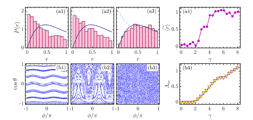
Figure 1: (a1)-(a3): Level spacing ratio probability distribution in Eq. (3) of the KT model for $\gamma=0.2$ (a1), $\gamma=2.3$ (a2), and $\gamma=7$ (a3) with $j=2000$. The dashed and solid curves in each panel denote $P_{P}(r)$ and $P_{WD}$ in (4), respectively. (a4) Averaged ratio $\widetilde{\langle r\rangle}$ [cf. Eq. (5)] of the KT model as a function of $\gamma$ for $j=2000$. (b1)-(b3): Classical phase space portraits of the KT model for $90$ random initial conditions with $\gamma=0.2,2.3$, and $\kappa=7$ [from (b1) to (b3)]. Each initial condition has been evolved for $300$ kicks. (b4) Phase space averaged Lyapunov exponent $\Lambda_{m}$ (7) of the KT model as a function of $\gamma$. Here, $\Lambda_{m}$ is numerically obtained by averaging over $2\times 10^{4}$ initial conditions, each evolved for $1\times 10^{5}$ kicks. Other parameter: $\beta=\pi/3$.

II Kicked top model

The kicked top (KT) model [28, 26], firstly introduced in the context of quantum chaos [29, 30, 31, 32, 33, 34, 35, 36, 37, 38], describes the periodic kicking on a precessing top with angular momentum $\mathbf{J}=(J_{x},J_{y},J_{z})$. This model has been extensively studied in many areas of physics [39, 40, 41, 42, 43, 44, 45, 46, 47, 48, 49] and can be realized in different experimental platforms [50, 51, 52]. The Hamiltonian of the KT model can be written as

$$H_{KT}=\beta J_{z}+\frac{\gamma}{2j}J_{x}^{2}\sum_{n=-\infty}^{+\infty}\delta(t-n),$$ (1)

where $\beta$ is the angular frequency of the precession around $z$ axis, $\gamma$ denotes the strength of the $\delta$ kicks with unit period, and $j$ quantifies the total magnitude of $\mathbf{J}$, so that $\mathbf{J}^{2}=j(j+1)$. Here, we set $\hbar=1$ throughout this work.

The conservation of $\mathbf{J}^{2}$ in the KT model allows us to work in the Dicke basis $|j,m\rangle$, defined by $j_{z}|j,m\rangle=m|j,m\rangle$ and $\mathbf{J}^{2}|j,m\rangle=j(j+1)|j,m\rangle$ with $-j\leq m\leq j$, and the dimension of the Hilbert space is $\mathcal{D}=2j+1$. Moreover, the Hamiltonian (1) also conserves the parity operator $\Pi=(-1)^{(j+J_{z})}$. Consequently, the Hilbert space can be further split into even- and odd-parity subspaces with dimensions $\mathcal{D}_{e}=j+1$ and $\mathcal{D}_{o}=j$ for even $j$. We focus on the even-parity subspace in this work and consider $j$ even.

It is known that the KT model exhibits a transition to chaos with increasing the kick strength [26, 37, 53, 54, 55]. The onset of chaos in the KT model can be analyzed through the spectral properties of the Floquet operator, which can be written as

$$\mathcal{F}=\exp\left(-i\frac{\gamma}{2j}J_{x}^{2}\right)\exp(-i\beta J_{z}).$$ (2)

By numerically diagonalizing $\mathcal{F}$ in the Dicke basis, we obtain its eigenvalues $\{\alpha_{k}\}\in[-\pi,\pi)$, also known as the quasienergies of the KT model. Then, we consider the level spacing ratios [56], defined as

$$r_{k}=\mathrm{min}\left(\delta_{k},\frac{1}{\delta_{k}}\right),$$ (3)

where $\delta_{k}=d_{k+1}/d_{k}$ with $d_{k+1}=\alpha_{k+1}-\alpha_{k}$ being the spacing between two nearest quasienergies. The presence of chaos can be revealed by the probability distribution of $r_{k}$, denoted by $P(r)$. It has been verified that for the regular and fully chaotic systems $P(r)$ are, respectively, captured by the Poisson and Wigner-Dyson distributions [57, 58, 59],

$$P_{P}=\frac{2}{(1+r)^{2}},\quad P_{WD}=\frac{27}{4}\frac{r+r^{2}}{(1+r+r^{2})^{5/2}}.$$ (4)

In Figs. 1(a1)-1(a3), we plot how $P(r)$ varies as $\gamma$ is increased. The crossover from $P_{P}(r)$ to $P_{WD}(r)$ with increasing $\gamma$ is clearly visible, indicating the occurrence of chaos at larger values of $\gamma$. Further confirmation of the transition to chaos is provided by the rescaled average ratio, defined by [37]

$$\widetilde{\langle r\rangle}=\frac{|\langle r\rangle-\langle r\rangle_{P}|}{\langle r\rangle_{WD}-\langle r\rangle_{P}}.$$ (5)

Here, $\langle r\rangle$ is the average of $r_{k}$, $\langle r\rangle_{P}=\int rP_{P}(r)dr\approx 0.39$, and $\langle r\rangle_{WD}=\int rP_{WD}(r)dr\approx 0.53$ [57]. The results in Figs. 1(a1)-1(a3) suggest that $\widetilde{\langle r\rangle}$ keeps its value around the zero for smaller values of $\gamma$, while it saturates near $\widetilde{\langle r\rangle}\approx 1$ when $\gamma$ is sufficient large. This is displayed in Fig. 1(a4), where the dependence of $\widetilde{\langle r\rangle}$ on $\gamma$ is shown.

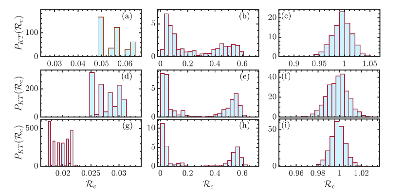
Figure 2: (a)-(c): Probability distribution, $P_{KT}(\mathcal{R}_{c})$, of $\mathcal{R}_{c}$ in Eq. (9) for $\gamma=0.2$ (a), $\gamma=2.3$ (b) and $\gamma=7$ (c) with $N_{k}=1000$. (d)-(f): $P_{KT}(\mathcal{R}_{c})$ for the same values of $\gamma$ as in panels (a)-(c) with $N_{k}=4000$. (g)-(i): $P_{KT}(\mathcal{R}_{c})$ for the same $\gamma$ values as in panels (a)-(c) with $N_{k}=8000$. Here, an ensemble of $1600$ initial conditions has been employed to calculate the probability distribution $P_{KT}(\mathcal{R}_{c})$. Other parameter: $\beta=\pi/3$.

The transition to chaos in (1) can be considered as a quantum manifestation of the chaotic motion in its classical counterpart. The classical KT model is described by the following classical map [37]

$$\begin{bmatrix}X_{n+1}\\ Y_{n+1}\\ Z_{n+1}\end{bmatrix}=\begin{pmatrix}\cos\beta&-\sin\beta&0\\ \sin\beta\cos\Theta_{n}&\cos\beta\cos\Theta_{n}&-\sin\Theta_{n}\\ \sin\beta\sin\Theta_{n}&\sin\beta\sin\Theta_{n}&\cos\Theta_{n}\end{pmatrix}\begin{bmatrix}X_{n}\\ Y_{n}\\ Z_{n}\end{bmatrix},$$ (6)

where $\Theta_{n}=\gamma(X_{n}\cos\beta-Y_{n}\sin\beta)$. The classical vector $\mathbf{X}=(X,Y,Z)$ satisfies $|\mathbf{X}|^{2}=X^{2}+Y^{2}+Z^{2}=1$. We thus parametrize $(X,Y,Z)$ as $X=\sin\theta\cos\phi,Y=\sin\theta\sin\phi$ and $Z=\cos\theta$, with $\theta,\phi$ being the azimuthal and polar angles, respectively. The classical phase space is characterized by canonical variables $\phi=\arctan(Y/X)$ and $\cos\theta$.

The classical phase portraits for several kick strengths are plotted in Figs. 1(b1)-1(b3). As $\gamma$ is increased, the phase space evolves from occupied by regular orbits ($\gamma=0.2$) to the celebrated Kolmogorov-Arnold-Moser scenario ($\gamma=2.3$), and to the almost entirely covered by chaotic trajectories, with invisible regular islands ($\gamma=7$). These observed features can be quantitatively captured by the phase space averaged Lyapunov exponent, defined by

$$\Lambda_{m}=\frac{1}{4\pi}\int\lambda_{m}\sin\theta d\theta d\phi.$$ (7)

Here, $\lambda_{m}$ is the largest Lyapunov exponent of the classical map (6) and it can be calculated as [29, 60] $\lambda_{m}=\ln[\lim_{n\to\infty}(\tau_{m})^{1/n}]$ with $\tau_{m}$ being the maximal eigenvalue of $\mathcal{T}=\prod_{s=1}^{n}(\partial\mathbf{X}_{s+1}/\partial\mathbf{X}_{s})$. The variation of $\Lambda_{m}$ as a function of $\gamma$ is shown in Fig. 1(b4). It is obvious that $\Lambda_{m}$ remains zero for $\gamma\lesssim 2$, due to the regularity of the model. However, it grows with increasing $\gamma$ as soon as $\gamma>2$, indicating the onset of chaos in the model. Here, it is worth mentioning that even though the transition to chaos in the KT model depends on the value of $\beta$ [61], the main results of this work are independent of it. This has been carefully checked in our studies. We thus fixed $\beta=\pi/3$ in the present work.

By comparing Fig. 1(a4) with 1(b4), we note that the upturns in $\widetilde{\langle r\rangle}$ and $\Lambda_{m}$ are in agreement with each other, suggesting a good quantum-classical correspondence. This is however expected in the infinite time limit, whether it still holds for finite time case remains unknown. In the rest of this section, we address this question in the KT model by exploring how the classical chaotic measure, defined through the finite time trajectories, relates to the degree of quantum chaos.

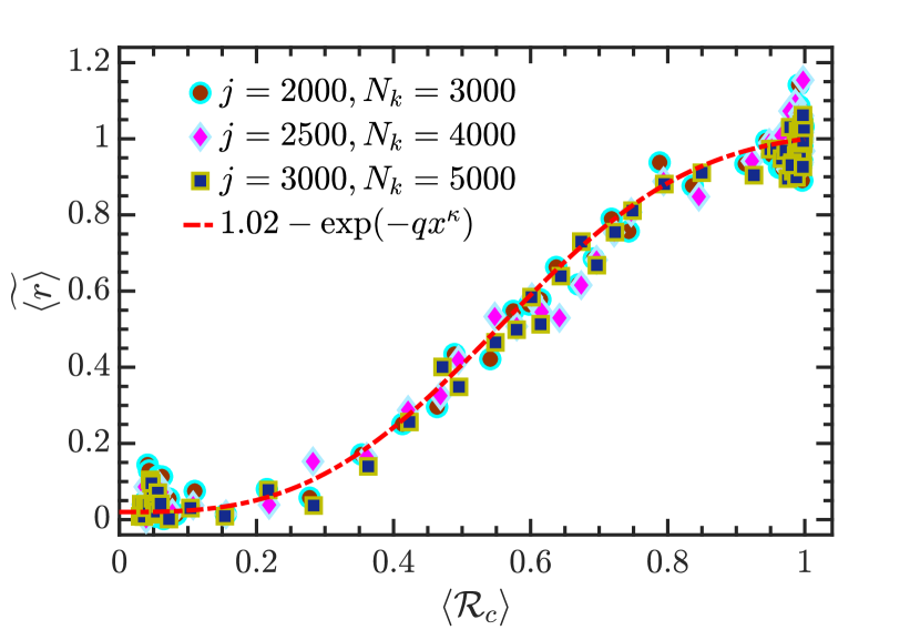
Figure 3: Quantum chaotic measure $\widetilde{\langle r\rangle}$ in (5) as a function of the finite time classical chaotic measure $\langle\mathcal{R}_{c}\rangle$ in (11) for the KT model with several values of $j$ and $N_{k}$. Here, $\langle\mathcal{R}_{c}\rangle$ is calculated by averaging over an ensemble with $1600$ initial conditions. The red dot-dashed curve denotes the best fitting of the data and it has the form $y=1.02-\exp(-qx^{\kappa})$ with $\kappa\approx 2.9892$ and $q\approx 3.8834$. Other parameter: $\beta=\pi/3$.

II.1 Dynamical chaos in KT model

The aim of our studying requires us to quantify the degree of chaos for a given finite time trajectory. To this end, we focus on a classical trajectory evolved for $N_{k}$ kicks. As a result, a finite time trajectory is described by $N_{k}$ points in the classical phase space. The distribution of these $N_{k}$ points in the phase space is strongly dependent on whether the classical dynamics is regular or chaotic. For regular dynamics, $N_{k}$ points should exhibit clustering and distribute with certain structures in the phase space. In contrast, the chaotic dynamics results in $N_{k}$ points being randomly scattered, leading to a structureless phase space.

To quantitatively capture above features exhibited by a finite time classical trajectory, we divide the phase space into $M_{c}$ cells with equal size, and consider the number of occupied cells $M_{p}$. Obviously, too small and/or too large value of $M_{c}$ are not allowed, as they will wipe out the difference between the regular and chaotic dynamics. The suitable value of $M_{c}$ can be determined via the approach proposed by Casati and coworkers [25]. According to their method, we need to define the Shannon entropy for a certain cell. As an arbitrary cell is either occupied or not occupied, the Shannon entropy of a cell can be defined as

$$S_{e}(M_{c})=-p\ln p-(1-p)\ln(1-p).$$ (8)

Here, $p=1-(1-1/M_{c})^{N_{k}}$ is the occupation probability of our considered cell for $N_{k}$ points that are randomly distributed over $M_{c}$ cells. Then, by maximizing the Shannon entropy with respect to $M_{c}$, one can find that the optimal value of $M_{c}$ is given by $M_{c}=N_{k}/\ln 2\approx N_{k}$. In the numerical simulation, one can take $M_{c}=N_{k}$ and define the measure of chaoticity of a finite time trajectory as

$$\mathcal{R}_{c}=\frac{M_{r}}{N_{k}},$$ (9)

where $M_{r}=M_{p}/(pM_{c})N_{k}$ is the normalized $M_{p}$. One can expect that $\mathcal{R}_{c}$ will have vanishingly small values for regular trajectories, while it has the order of magnitude $O(1)$ for the chaotic trajectories.

We find that $\mathcal{R}_{c}$ in (9) indeed enables us to quantify the degree of chaos of the finite time trajectories, as confirmed by its probability distribution for an ensemble of initial conditions, defined by

$$P_{KT}(\mathcal{R}_{c})=\frac{1}{\mathcal{N}_{s}}\sum_{u=1}^{\mathcal{N}_{s}}\delta(\mathcal{R}_{c}-\mathcal{R}_{c,u}),$$ (10)

where $\mathcal{N}_{s}$ is the number of initial conditions in the given ensemble. The regular behavior for the classical trajectories gives rise to vanishingly small values of $\mathcal{R}_{c}$, as both the average and fluctuation of $P_{KT}(\mathcal{R}_{c})$ are tiny, while the chaotic trajectories would result in a narrow distribution $P_{KT}(\mathcal{R}_{c})$ around $\mathcal{R}_{c}\simeq 1$.

In Fig. 2, we show how $P_{KT}(\mathcal{R}_{c})$ varies for several values of $\gamma$ and $N_{k}$. On the one hand, as seen in the first column of Fig. 2, $P_{KT}(\mathcal{R}_{c})$ has small average value and width in the regular regime, regardless of the number of kicks. Moreover, we see that the average and width of $P_{KT}(\mathcal{R}_{c})$ decrease with increasing $N_{k}$. We thus expect that $P_{KT}(\mathcal{R}_{c})$ will become a delta distribution located at $\mathcal{R}_{c}=0$ in the limit $N_{k}\to\infty$. On the other hand, in the chaotic case, the distribution $P_{KT}(\mathcal{R}_{c})$ exhibits a concentration with an average value close to $1$, as demonstrated in the last column of Fig. 2. Similar to the regular case, the width of $P_{KT}(\mathcal{R}_{c})$ for the chaotic trajectories also decreases when we increase $N_{k}$. In the limit $N_{k}\to\infty$, one can expect that $P_{KT}(\mathcal{R}_{c})$ will take the form $P_{KT}(\mathcal{R}_{c})=\delta(\mathcal{R}_{c}-1)$. For the mixed regime, as shown for the case of $\gamma=2.3$ in the second column of Fig. 2, the distribution $P_{KT}(\mathcal{R}_{c})$ is characterized by double peak shape. Two peaks in $P_{KT}(\mathcal{R}_{c})$ are, respectively, corresponding to the regular and chaotic trajectories. We further note that the smoothness of $P_{KT}(\mathcal{R}_{c})$ is enhanced by increasing $N_{k}$.

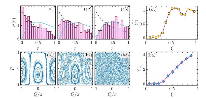
Figure 4: (a1)-(a3): Probability distribution, $P(r)$, of the level spacing ratio (3) of the Dicke model for $\xi=0.1$ (a1), $\xi=0.3$ (a2), and $\xi=1$ (a3) and energy levels $E_{k}\in[1.05,1.22]$ with $N=80$. The dashed and solid curves in each panel denote $P_{P}(r)$ and $P_{WD}$ in (4), respectively. (a4) Rescaled averaged ratio $\widetilde{\langle r\rangle}$ in (5) of the Dicke model for the energy levels $E_{k}\in[1.05,1.22]$ as a function of $\xi$ with $N=80$. (b1)-(b3): Classical Poincaré sections in $(P,Q)$ plane of the Dicke model for $81$ random initial conditions with $\xi=0.1,0.3$, and $\xi=1$ [from (b1) to (b3)] and a fixed energy $\mathcal{E}=1.2$. Each initial condition has been evolved for $t=3000$. (b4) Phase space averaged Lyapunov exponent $\Upsilon_{m}$ (7) of the Dicke model as a function of $\xi$. Here, $\Upsilon_{m}$ is numerically obtained by averaging over $5000$ initial conditions, each evolved for $t=1\times 10^{3}$. Other parameters: $\omega=\omega_{0}=1$.

Above features of $P_{KT}(\mathcal{R}_{c})$ justify the correctness of $\mathcal{R}_{c}$ for measuring the chaoticity of the finite time classical trajectories. They also imply that the degree of chaos for classical KT model in a finite time can be quantified by the average of $\mathcal{R}_{c}$, defined by

$$\langle\mathcal{R}_{c}\rangle=\sum_{u}\mathcal{R}_{c,u}P_{KT}(\mathcal{R}_{c}).$$ (11)

To see whether the quantum-classical correspondence still holds in finite time, we examine the dependence between $\langle\mathcal{R}_{c}\rangle$ and the measure of quantum chaos, given by $\widetilde{\langle r\rangle}$ in Eq. (5). In Fig. 3, we show how $\widetilde{\langle r\rangle}$ correlates with $\langle\mathcal{R}_{c}\rangle$ for different values of $j$ and $N_{k}$. The collapse of data is clearly visible, indicating that the behavior of $\widetilde{\langle r\rangle}$ is in good agreement with $\langle\mathcal{R}_{c}\rangle$. In particular, a numerical fitting shows that the variation of $\widetilde{\langle r\rangle}$ with $\langle\mathcal{R}_{c}\rangle$ can be well captured by a function of the form

$$y=1.02-\exp(-qx^{\kappa}),$$ (12)

which has been plotted as the red dot-dashed curve in Fig. (3). For the KT model, we have found that $\kappa\simeq 2.9892$ and $q\simeq 3.8834$ are independent of the values of $j$ and $N_{k}$.

These results not only verify the usefulness of $\mathcal{R}_{c}$ for measuring the chaoticity of the finite time trajectories, but also reveal that the quantum-classical correspondence still holds for the finite time case. However, as the KT model is a single particle system, further investigation of quantum many-body systems is required in order to strengthen above statement. We thus proceed to perform an analysis in the celebrated Dicke model.

III Dicke model

The Dicke model consists of an ensemble of $N$ spin-$1/2$ atoms interacting with a single bosonic mode [27, 62] and plays a fundamental role in a wide range of fields, including various phase transitions [63, 64, 65, 66, 67, 68, 69, 70, 71, 72, 73, 74, 75, 76], quantum chaos and thermalization [76, 77, 78, 79, 80, 81, 82, 83, 84, 85, 86, 87, 88, 89], and information scrambling [90, 91]. It has also been applied to understand several critical phenomena observed in different experimental platforms [92, 93, 94]. A very recent review on the properties and applications of the Dicke model can be found in Ref. [95].

The Hamiltonian of the Dicke model can be written as

$$H_{D}=\omega a^{\dagger}a+\omega_{0}J_{z}+\frac{2\xi}{\sqrt{N}}(a+a^{\dagger})J_{x},$$ (13)

where $\omega$, $\omega_{0}$, and $\xi$ correspond to the frequency of the bosonic mode, energy splitting of atoms, and the strength of atom-field interaction. The bosonic annihilation (creation) operator is denoted by $a$ ($a^{\dagger}$), while $J_{a}(a=x,y,z)$ are the collective spin-$1/2$ operators along $a$ axis and satisfy the $\mathrm{SU}(2)$ commutation relations.

As the Hamiltonian $H_{D}$ (13) commutes with $\mathbf{J}^{2}=\sum_{a}J_{a}^{2}$, one can divide the Hilbert space into different subspaces distinguished by the eigenvalues of $\mathbf{J}^{2}$, given by $j(j+1)$. We restrict ourselves in the subspace with $j=N/2$ and the dimension of the Hilbert space is $\mathcal{D}=(N+1)(\mathcal{N}_{tr}+1)$ with $\mathcal{N}_{tr}$ being the truncation number of the bosonic mode. Moreover, the conservation of the parity $\Pi=(-1)^{j+J_{z}+a^{\dagger}a}$ for $H_{D}$ enables us to further separate the Hilbert space into even- and odd-parity subspaces. In this work, we focus on the even-parity subspace, so that the dimension of the Hilbert is given by $\mathcal{D}_{e}=(N/2+1)(\mathcal{N}_{tr}+1)-\mathcal{N}_{tr}/2$ for even $N$. The requirement of the convergence of the numerical results leads us to take $\mathcal{N}_{tr}=380$. We have carefully checked that our results are unchanged for increasing $\mathcal{N}_{tr}$.

Several interesting features have been found in the Dicke model. Among them, the transition to chaos is an intriguing topic and has been triggering many endeavors to explore it, from both static [76, 80, 82, 81, 96, 97] and dynamical aspects [84, 91, 98, 99, 100, 101]. Generally speaking, the spectral statistics of $H_{D}$ turns from the Possion statistics to the Wigner-Dyson statistics around $\xi_{c}\simeq\sqrt{\omega_{0}\omega}/2$. However, a detailed study reveals that the precise value of $\xi_{c}$ also strongly depends on the energy [82, 85, 102].

In Figs. 4(a1)-4(a3), we show how the distribution of level spacing ratio $r_{k}$ in (3), $P(r)$, varies with increasing $\xi$ for the energies $E_{k}\in[\bar{E}-0.15,\bar{E}+0.02]$ with $\bar{E}=1.2$ and the system size $N=80$. We see that $P(r)$ undergoes an obvious crossover from the Possion distribution to the Wigner-Dyson distribution as $\xi$ is increased, suggesting the onset of chaos at larger values of $\xi$. Moreover, as we focus on the energy levels with higher energies, $P(r)$ displays a visible deviation from $P_{P}(r)$ at $\xi<\sqrt{\omega_{0}\omega}/2$, as observed in Fig. 4(a2). The transition to chaos with increasing $\xi$ is more clearly revealed by the upturn in the rescaled averaged level spacing ratio $\widetilde{\langle r\rangle}$ around $\xi\sim 0.2$, as seen in Fig. 4(a4).

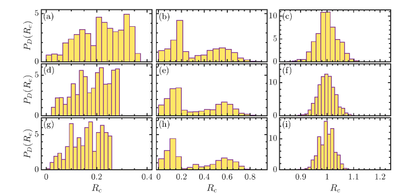
Figure 5: (a)-(c): Probability distribution, $P_{D}(R_{c})$, of $R_{c}$ in Eq. (19) for $\xi=0.1$ (a), $\xi=0.3$ (b) and $\xi=1$ (c) with $T_{m}=1000$. (d)-(f): $P_{D}({R}_{c})$ for the same values of $\xi$ as in panels (a)-(c) with $T_{m}=1500$. (g)-(i): $P_{D}({R}_{c})$ for the same $\xi$ values as in panels (a)-(c) with $T_{m}=2000$. Here, $T_{m}$ denotes the evolution time of our considered trajectories and an ensemble of $1600$ initial conditions has been employed to calculate the probability distribution $P_{D}(R_{c})$. Other parameters: $\omega=\omega_{0}=1$ and the traversal time $T_{r}\simeq 6.2$.

As in the KT model, the presence of chaos in $H_{D}$ can be understood as a quantum analogue of the classical chaos. The classical counterpart of the Dicke model is obtained by calculating the expectation value of $H_{D}$ in the tensor product state $|CS\rangle=|\alpha\rangle\otimes|z\rangle$ [103]. Here, $|\alpha\rangle$ and $|z\rangle$ are the Glauber and Bloch coherent states, defined by [104]

$$|\alpha\rangle=e^{-|\alpha|^{2}}e^{\alpha a^{\dagger}}|0\rangle,\quad|z\rangle=\frac{1}{(1+|z|^{2})^{j}}e^{zJ_{+}}|j,-j\rangle,$$ (14)

where $\alpha,z\in\mathbb{C}$, $|0\rangle$ is the vacuum state of the bosonic mode, $J_{+}=J_{x}+iJ_{y}$, and $|j,-j\rangle$ fulfills $J_{z}|j,-j\rangle=-j|j,-j\rangle$. We parametrize $\alpha,z$ as [80, 81]

$$\alpha=\sqrt{\frac{j}{2}}(q+ip),\quad z=\sqrt{\frac{1+P}{1-P}}e^{iQ},$$ (15)

where $(p,q)\in\mathbb{R}^{2}$ are the canonical variables of the bosonic sector, while $(P,Q)\in\mathbb{R}^{2}$ with $-1\leq P\leq 1,-\pi\leq Q\leq\pi$ represent the canonical variables of the atomic sector. Then, the classical Hamiltonian of the Dicke model can be written as

$$\mathcal{H}_{D}^{c}=\frac{\langle CS|H_{D}|CS\rangle}{j}=\omega_{0}P+\frac{\omega}{2}(p^{2}+q^{2})+2\xi q\cos Q\sqrt{1-P^{2}}.$$ (16)

Consequently, the classical equations of motion (CEM) are given by

$$\dot{q}=\omega p,\ \dot{p}=-\omega q-2\xi\cos Q\sqrt{1-P^{2}},$$

$$\dot{Q}=\omega_{0}-\frac{2\xi qP\cos Q}{\sqrt{1-P^{2}}},\ \dot{P}=2\xi q\sin Q\sqrt{1-P^{2}}.$$ (17)

with the initial condition $(p_{0},q_{0},P_{0},Q_{0})$.

The chaos presented by $\mathcal{H}_{D}^{c}$ in (16) with increasing $\xi$ can be uncovered using the Poincaré section. To define the Poincaré section at certain energy $\mathcal{E}$, we consider a plane with $p=0$. As the energy of the system is conserved, i. e. $\mathcal{H}_{D}^{c}(p=0,q,P,Q)=\mathcal{E}$, this plane is actually characterized by the variables $(P,Q)$. The Poincaré section is then defined as the intersection of the classical trajectories with this surface.

In Figs. 4(b1)-4(b3), we plot Poincaré sections for different values of $\xi$ with energy $\mathcal{E}=1.2$. For smaller values of $\xi$, such as the one shown in Fig. 4(b1), the Poincaré section is dominated by regular structure, indicating the regular dynamics in the classical Dicke model. This is in good agreement with quantum case in Fig. 4(a1). When the value of $\xi$ increases the chaotic trajectories appear, leading to a mixed Poincaré section in which the regular islands are coexisting with a chaotic sea, as exemplified in Fig. 4(b2) for the case of $\xi=2.3$. As $\xi$ is further increased, e. g. $\xi=1$ case depicted in Fig. 4(b3), the Poincaré section is fully covered by chaotic trajectories, although there may still exist several invisible regular islands.

To quantify the chaotic behavior in the Dicke model, we consider the phase space averaged Lyapunov exponent, defined by

$$\Upsilon_{m}=\int u_{m}(P,Q)d\mathcal{A},$$ (18)

where $d\mathcal{A}=dPdQ$ is the area element of the phase space. Here, $u_{m}(P,Q)$ is the largest Lyapunov exponent and can be calculated through the numerical approach in Refs. [82, 102]. In Fig. 4(b4), we plot $\Upsilon_{m}$ as a function of $\xi$ with $\mathcal{E}=1.2$. For small values of $\xi$, $\Upsilon_{m}$ stays vanishingly small until $\xi\sim 0.2$, from which it starts to grow as $\xi$ is increased, indicating the onset of chaos. It is worth pointing out that the behavior of $\widetilde{\langle r\rangle}$ is in good agreement with $\Upsilon_{m}$.

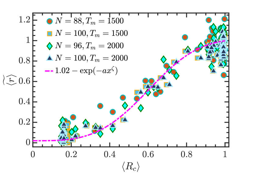
Figure 6: Quantum chaotic measure $\widetilde{\langle r\rangle}$ in (5) as a function of the finite time classical chaotic measure $R_{c}$ in (21) for the Dicke model with several values of the system sizes $N$ and $T_{m}$. Here, $T_{m}$ is the evolution time of the classical trajectories and $R_{c}$ is calculated by averaging over an ensemble with $1600$ initial conditions. Moreover, $\widetilde{\langle r\rangle}$ are calculated for the energy levels that satisfy $E\in[\bar{E}-0.15,\bar{E}+0.02]$ with $\bar{E}=1.2$. The magenta dot-dashed curve denotes the best fitting of the data and it has the form $y=1.02-\exp(-ax^{\zeta})$ with $\zeta\approx 3.3885$ and $a\approx 3.8328$. Other parameters: $\omega=\omega_{0}=1$.

Different from the KT model, the classical dynamics of the Dicke model depends on the energy of the model. This requires us to consider the energy shell in which the underlying classical dynamics should not be changed. The energy shell studied in this work is defined by $E_{k}\in[\bar{E}-0.15,\bar{E}+0.02]$ with $\bar{E}=1.2$. We have checked that there are no substantial variations in the corresponding classical dynamics for this energy interval. Moreover, we would also like to point out that our main results still hold for other choice of energy shells, as long as the classical dynamics keeps unchanged in the chosen energy shell.

Here, we see again a good correspondence between the classical and quantum chaotic features in the Dicke model. As we have pointed out in the KT model, this correspondence is expected in the infinite time limit. In order to get more insights into the correspondence principle in the studies of quantum chaos, it is also necessary to explore the connection between the quantum and classical chaotic properties in the finite time.

III.1 Dynamical chaos in Dicke model

As we have done in the KT model, the chaoticity of the finite time trajectories in the Dicke model is also measured through the characters of the points in the Poincaré section. However, different from the KT model, the classical dynamics of the Dicke model is governed by the differential equations, rather than the mapping. Hence, it is required to determine how many points of a classical trajectory evolved up to time $T_{m}$ are taken in the Poincaré section. By defining the time between two successive crossings of the Poincaré section as the traversal time $T_{r}$, the number of points in the Poincaré section for a trajectory with $T_{m}$ iterations is $N_{m}=T_{m}/T_{r}$.

Similar to the KT model, the distribution features of these $N_{m}$ points in the Poincaré section depend on the chaoticity of the trajectory. To analyze the chaotic behavior of a finite time trajectory, we also discretize the Poincaré section into a grid of $M_{d}$ cells, and count how many cells are occupied for a given trajectory. This means that there exists an optimal value of $M_{d}$. Following the same discussion as in the KT model, it is easy to show that the best choice of $M_{d}$ is given by $M_{d}=N_{m}/\ln 2\simeq N_{m}$. We thus define the chaotic measure of a finite time trajectory as

$$R_{c}=\frac{N_{R}}{N_{m}},$$ (19)

where $N_{R}=M_{R}/(pM_{d})N_{m}$ with $M_{R}$ being the number of occupied cells and $p=1-(1-1/M_{d})^{N_{m}}$.

Let us first focus on the distribution of $R_{c}$ for an ensemble of initial conditions, defined by

$$P_{D}(R_{c})=\frac{1}{\mathcal{M}_{s}}\sum_{v=1}^{\mathcal{M}_{s}}\delta(R_{c}-R_{c,v}),$$ (20)

where $\mathcal{M}_{s}$ denotes the number of initial conditions in an ensemble. The variation of $P_{D}(R_{c})$ for an ensemble of $1600$ initial conditions with different values of $\xi$ and $T_{m}$ has been illustrated in Fig. 5. An overall similarities between Fig. 2 and Fig. 5 can be clearly identified. Specifically, since the points in the Poincaré section are clustered for the trajectories with regular dynamics, the distribution $P_{D}(R_{c})$ is supported over the smaller values of $R_{c}$ and its width decreases with increasing $T_{m}$, as seen in the first column of Fig. 5. This behavior of $P_{D}(R_{c})$ leads us to expect that it would turn to $P_{D}(R_{c})=\delta(R_{c})$ as $T_{m}$ goes to infinity, and the same trend is also presented in the KT model. On the contrary, as the trajectories with chaotic dynamics result in randomly scattered points in Poincaré section, $P_{D}(R_{c})$ is well described by a narrow distribution around $R_{c}\simeq 1$, as shown in the last column of Fig. 5. We further note that the distribution of $R_{c}$ for the chaotic trajectories becomes more and more narrow as $T_{m}$ is increased, suggesting $P_{D}(R_{c})$ approaches a delta distribution centered at $R_{c}=1$ in the $T_{m}\to\infty$ limit, as exhibited by the KT model. The coexistence of the regular and chaotic trajectories in the mixed regime gives rise to the double peak shape of $P_{D}(R_{c})$, as demonstrated in the middle column of Fig. 5. As observed in the KT model, the smoothness of $P_{D}(R_{c})$ can be improved by enhancing $T_{m}$.

After verifying the ability of $R_{c}$ in (19) to capture the chaotic degree of the finite time trajectories, we continue to analyze the validity of the quantum-classical correspondence in the Dicke model for finite time trajectories. According to the results in the KT model, the chaoticity of the classical Dicke model in finite time can be measured by averaging $R_{c}$ over an ensemble,

$$\langle R_{c}\rangle=\sum_{v=1}^{\mathcal{M}_{s}}R_{c,v}P_{D}(R_{c}),$$ (21)

while the degree of quantum chaos is quantified through $\widetilde{\langle r\rangle}$ [cf. Eq. (5)] in a given energy shell. The correspondence between the quantum and classical chaoticity measures indicates that the variation of $\widetilde{\langle r\rangle}$ should depend strongly on $\langle R_{c}\rangle$.

The variation of $\widetilde{\langle r\rangle}$ as a function of $\langle R_{c}\rangle$ for several system sizes $N$ and evolution times $T_{m}$ in the Dicke model is shown in Fig. 6. The resemblance between Figs. 3 and 6 is clearly visible. However, as the system size and evolution time that can be approached in our numerical simulation of the Dicke model are much smaller than in the KT model, the results for the Dicke model have larger fluctuations, as compared to Fig. 3. Nevertheless, one can see that the fluctuations can be suppressed by increasing $N$ and/or $T_{m}$. In particular, as marked by the magenta dot-dashed curve in Fig. 6, the dependence of $\widetilde{\langle r\rangle}$ on $\langle R_{c}\rangle$ is captured by the same function as in the KT model, i. e. $y=1.02-\exp(-ax^{\zeta})$. For the Dicke model, we obtain $\zeta\simeq 3.3885,a=3.8328$, which are remarkably close to the corresponding values in the KT model. Almost the same relationship between the quantum and classical chaotic measures has been observed in two totally different quantum systems. This fact not only confirms that the correspondence principle also holds for the finite time trajectories, but also leads us to expect that our main findings may still be valid for other quantum many-body systems with well-defined classical limit.

IV Conclusions

In this work, we have studied how to measure the degree of chaos for finite time trajectories and examined the quantum-classical correspondence in two different quantum systems, namely kicked top and Dicke models. By utilizing the distinct features exhibited by the regular and chaotic trajectories in the Poincaré section, we have shown how to quantify the degree of chaos for a finite time classical trajectory. The correctness of our defined finite time chaotic measure has been verified through a detailed analysis of its probability distribution in our considered models. We have demonstrated that the transition to chaos leaves a strong imprint on the statistical properties of the finite time chaotic measure. Identifying the average of level spacing ratio as the measure of quantum chaos, we have explored the correspondence between the quantum and finite time classical chaoticities in both kicked top and Dicke models. Notably, the dependence of quantum chaotic measure on its classical counterpart can be well described by a simple function, which is independent of the model.

Our findings shed more light on the meaning of quantum-classical correspondence and provide a quantitative way to understand how the chaos develops with increasing time. The analytical expression of the relation between quantum and classical chaotic measures is independent of specific model. This indicates a general standard for ascertaining the quantum-classical correspondence. Moreover, the results of this work not only extend the conclusions of previous work [25], but also enhance our comprehending of quantum statistical physics.

A natural extension of the present work is to systematically investigate whether the quantum and finite time classical chaotic measures have the same relationship as in this work also in other quantum systems with well-defined classical counterpart. We expect that the results of these explorations will align with our conclusions. Another interesting question should be the analytical explanation of why the quantum chaotic measure exhibits the same dependence on the classical measure for different models. It would also be intriguing to examine how the finite time chaotic measure links to other quantum chaotic indicators and particularly the dynamical ones, such as spectral form factor [105] and Krylov complexity [106, 107].