Latent 3D Brain MRI Counterfactual

Abstract

The number of samples in structural brain MRI studies is often too small to properly train deep learning models. Generative models show promise in addressing this issue by effectively learning the data distribution and generating high-fidelity MRI. However, they struggle to produce diverse, high-quality data outside the distribution defined by the training data. One way to address the issue is using causal models developed for 3D volume counterfactuals. However, accurately modeling causality in high-dimensional spaces is a challenge so that these models generally generate 3D brain MRIS of lower quality. To address these challenges, we propose a two-stage method that constructs a Structural Causal Model (SCM) within the latent space. In the first stage, we employ a VQ-VAE to learn a compact embedding of the MRI volume. Subsequently, we integrate our causal model into this latent space and execute a three-step counterfactual procedure using a closed-form Generalized Linear Model (GLM). Our experiments conducted on real-world high-resolution MRI data (1mm) demonstrate that our method can generate high-quality 3D MRI counterfactuals.

1 Introduction

Generative AI models have demonstrated great potential to advance numerous medical fields including neuroimaging with 3D brain MRIs [18, 22]. The synthesis of medical images is particularly promising for tasks like improving image quality, imputing missing modalities [32], and modeling disease progression [31, 7, 8]. Recent advances in diffusion probabilistic models (DPMs) [6, 24] have played a significant role in this development as they are able to accurately capture the underlying data distributions. This results in synthesized medical images containing a great amount of detail [28, 11] that also differ from the training samples [9, 30]. Nevertheless, a key challenge remains generating realistic samples that are outside the distribution defined by the training dataset [10]. Overcoming this challenge is essential to the generalizability of large-scale models [30]. One way to address this shortcoming is by incorporating causality between factors during the generation progress [17]. For example, aging causes a thinning of the cortex that is accelerated in those with alcohol use disorder or Alzheimer’s disease, which provides a causal interaction not taken into account by statistical models. Here, we propose to integrate causality in the synthesis of 3D brain MRIs so that their generation can be guided by (interventions on) factors such as age, brain regions, and diagnosis.

Specifically we rely on probabilistic Structural Causal Model (SCM) [17, 19], which can incorporate the relationships between variables, directed from cause to effect. It indicates that intervening on a cause should lead to changes in the effect, rather than the other way around. This forces the model to consider our premises and assumptions about causality [3]. Contrary to previous SCMs [15, 29], we focus on the synthesis of 3D high-fidelity image counterfactuals of real-world data. However, building an SCM in a high-dimensional space presents considerable computational challenges, particularly when dealing with voluminous 3D MRIs. To that end, we build a counterfactual model that can learn the causality and perform counterfactual generation in a latent space, which allows us to produce 3D brain MRIs of higher quality than other counterfactual models.

Our model first employs a VQ-VAE [14] to encode the high-dimensional 3D brain MRI into a low-dimensional latent space. We then integrate a causal graphical model [3, 16] into this latent space such that interventions are performed in the latent space rather than the observation space (which contains MRIs). The three-step counterfactual procedure, i.e., abduction, action, and prediction, is subsequently achieved by a Generalized linear Model (GLM) [13] with a closed-form solution.

To the best of our knowledge, this is the first work that can perform high-fidelity counterfactual generation of 3D MRIs. Our counterfactual generative model does not only improve interpretability and generative performance but can also diversify (MRI) datasets. Additionally, counterfactual explanations could be key for preventive purposes, as it is inherently capable of showing how one’s brain might change under certain ‘conditions’ such as prolonged substance use. Our main contributions can be summarised as follows:

• We present a novel causal generative modeling framework in a latent space for producing high-fidelity 3D MRI counterfactuals with Markovian probabilistic causal models;

• Our model fulfills all three rungs of Pearl’s ladder of causation and the three-step procedure of the counterfactual generation can be realized efficiently by a novel GLM method;

• We show that our model can perform high fidelity 3D counterfactual generation and also demonstrate its axiomatic soundness of our counterfactuals by evaluating its context-level generation.

2 Methodology

Our method comprises a two-stage process (outlined in Fig. 1) that performs counterfactual generation of MRIs given attributes, e.g., age and brain regions of interest (ROIs). Given an intervention on (at least) one of these attributes, a Deep Structural Causal Model (DSCM) deploys a causal graph to compute the counterfactual of the attributes. For example, consider a brain MRI scan of an 80-year-old female, from which we extract the attributes age=80, sex=female, and the two ROI scores ROI_1_score=0.3 and ROI_2_score=0.7. Now to generate the brain MRI at age 50 years old, we intervene and set age=50, after which the DSCM computes the counterfactual attribute values, e.g., age=50, sex=male, ROI_1_score=0.4 and ROI_2_score=0.6. These counterfactual attributes are then used to compute the counterfactual feature embeddings, which are fed into a VQ-VAE decoder [14] in order to generate the corresponding MRI. These two stages are discussed below.

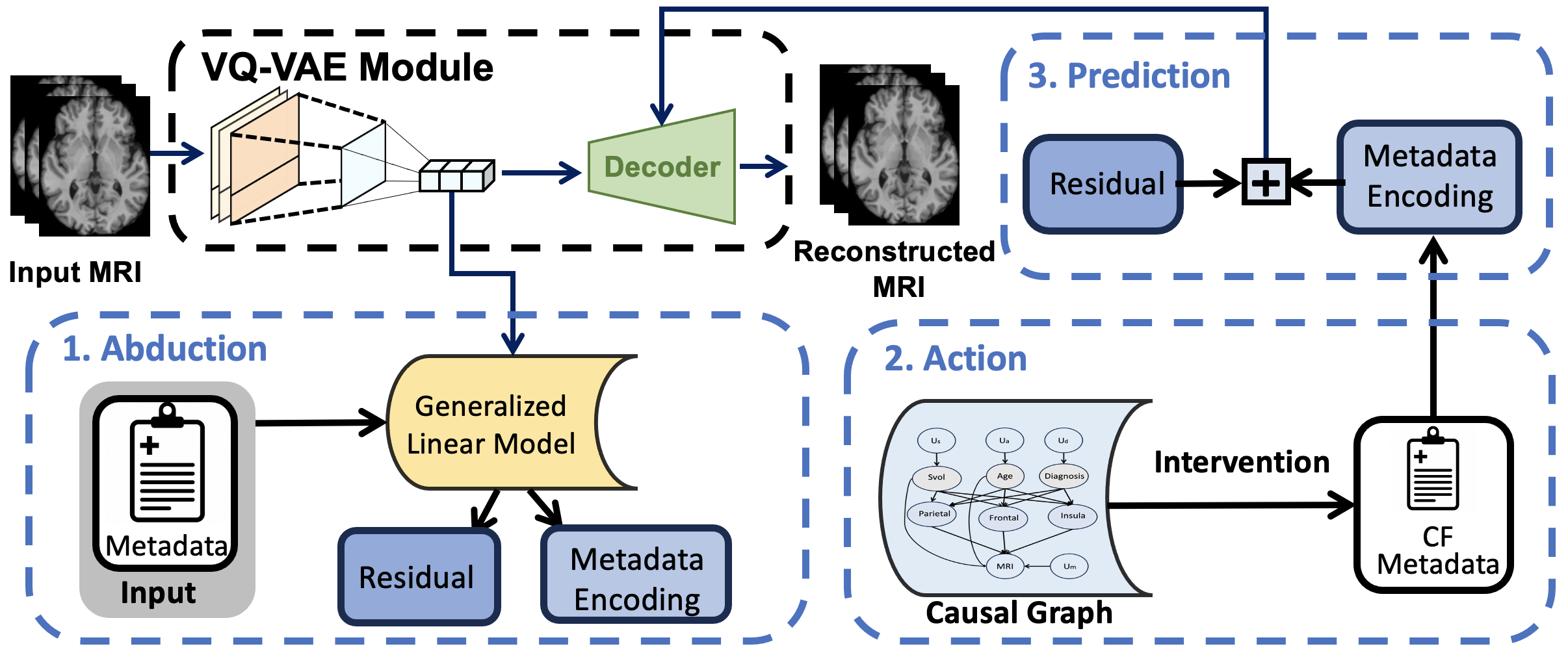
Figure 1: Architecture of the LSCM for image: Stage I (black box) consists of a VQ-VAE to encode the real 3D MRI to a quantized vector representation. Based on this, in stage II (blue boxes), a Latent SCM is constructed. The three-step procedure of counterfactual inference is achieved by a efficient GLM.

2.1 Deep Structural Causal Models

A structural causal model (SCM) [17] is a triple $\mathcal{M}\coloneqq\langle U,V,F\rangle$ consisting of two sets of variables: (i) exogenous variables $U=\{u_{1},\dots,u_{N}\}$; (ii) endogenous variables $V=\{v_{1},\dots,v_{N}\}$, and a set of functions known as causal mechanisms $F=\{f_{1},\dots,f_{N}\}$, which determine the values of the endogenous variables: $v_{k}:=f_{k}(\mathbf{pa}_{k},u_{k})$, where $\mathbf{pa}_{k}$ are the direct causes (parents) of $v_{k}$. It is possible to perform an intervention on any $v_{k}$ by, e.g., setting it to a constant $do(v_{k}\coloneqq c)$ and thereby disconnect $v_{k}$ from its causal parents. SCMs enable the estimation of counterfactuals (hypothetical scenarios) via a three-step process: (i) abduction: infer the posterior distribution $P(U\mid X)$, which represents the current state of the world; (ii) action: perform one or more interventions to obtain a modified model; (iii) prediction: infer counterfactual values of the endogenous variables using the modified model and the posterior $P(U\mid X)$.

In this work, we use a deep structural causal model (DSCM) [15] to model the causal relationships between patient attributes such as age, brain regions of interest, and diagnosis. Following [4], a DSCM uses a conditional normalizing flow [23] as the mechanism for each endogenous variable $v_{k}:=f_{k}({u}_{k};\mathbf{pa}_{k})$, to enable tractable and explicit abduction of the exogenous noise $u_{k}=f_{k}^{-1}(v_{k};\mathbf{pa}_{k})$. DSCMs can thereby tractably estimate counterfactuals given observed attributes and intervention(s). The counterfactual of any $v_{k}$ is given by
$\widehat{v}_{k}\coloneqq f_{k}(f_{k}^{-1}(v_{k};\mathbf{pa}_{k});\mathbf{\widehat{pa}}_{k})$, where $\mathbf{\widehat{pa}}_{k}$ are the counterfactual parents of $v_{k}$ resulting from an upstream intervention.

However, it has been shown that directly applying DSCMs [15] to 3D brain MRIs is impractical due to the complexity of constructing and optimizing invertible neural networks [27, 23]. Therefore, we separate the MRI variables $\mathbf{x}$ from $V$ and learn its counterfactual in a low dimensional latent space. For this purpose we adapt the Latent Structural Causal Model (LSCM) to 3D brain MRIs. We achieve this by using a generalized linear model (GLM) [13] in the latent space of a VQ-VAE model. After estimation of all counterfactual attributes, we obtain the counterfactuals of image latent features $\mathbf{z}$’s parents (see next section for details of $\mathbf{z}$), i.e. $\mathbf{\widehat{pa}_{z}}$, which will be used to generate $\widehat{\mathbf{z}}$. The resulting counterfactual feature encoding is converted into an MRI using the decoder of the VQ-VAE model.

2.2 Latent SCM for 3D Counterfactual MRIs

To fully leverage the latent SCM described in Section 2.1, a high-dimensional MRI $\mathbf{x}$ first has to be encoded to a corresponding latent feature $\mathbf{z}$, for which we use a VQ-VAE. Then, we obtain its counterfactual $\mathbf{\widehat{z}}$ based on $\mathbf{\widehat{pa}_{z}}$, which is finally decoded to the MRI counterfactual $\mathbf{\widehat{x}}$. We now discuss the process of obtaining these latent features $\mathbf{z}$ and estimating the counterfactuals $\mathbf{\widehat{z}}$, after which decoding is trivial given a trained VQ-VAE.

Computing latent feature $\mathbf{z}$.

To obtain a latent feature $\mathbf{z}$ from a 3D MRI $\mathbf{x}$, we employ a Variational Autoencoder (VQ-VAE) [14]. VQ-VAEs comprise an encoder $\mathcal{E}$ and decoder $\mathcal{D}$, as well as a code book $\mathcal{C}$ that performs vector quantisation (VQ). That is, code book $\mathcal{C}$ empowers mapping a 3D MRI $\mathbf{x}$ to a quantized encoding.

The first step in the process of computing the latent feature $\mathbf{z}$ is using the encoder $\mathcal{E}$ to map the 3D MRI $\mathbf{x}\in\mathbb{R}^{D\times H\times W}$ to its lower-dimensional feature representation $\mathbf{z}\coloneqq\mathcal{E}(\mathbf{x})\in\mathbb{R}^{d\times h\times w\times n_{D}}$. Correspondingly, the decoder $\mathcal{D}$ aims to reconstruct a 3D MRI $\hat{\mathbf{x}}=\mathcal{D}(\mathbf{z})$ from a compressed embedding $\mathbf{z}$. The training objective of the model is to minimize the reconstruction error. Once latent feature $\mathbf{z}$ is obtained, we apply vector quantization, which discretizes the continuous latent space using a set of embedding units $\mathcal{C}\coloneqq\{(k,e(k)):k=1,2,\ldots,N_{\mathcal{C}}\mbox{ and }e(k)\in\mathbb{R}^{n_{D}}\}$. This allows an MRI to be represented very efficiently by a set of indices (a.k.a. code) as defined with respect to the code book. Notably, this process also serves a regularization purpose to avoid overfitting the model during training.

After the encoding and vector quantization steps are finished, the latent representation $\mathbf{z}$ is described by $d\times h\times w$ vectors of $n_{D}$ dimensions each. This is achieved by searching the nearest neighbor of the embedding units in codebook $\mathcal{C}$ for each feature vector in $z_{c}$. In other words, each of the $d\times h\times w$ vectors $z_{c}\in\mathbb{R}^{n_{D}}$ from $\mathbf{z}$ is paired with its closest representative $e(k)$ from the codebook such that the corresponding code (a.k.a. index) is $\mathcal{I}(z_{c}):=\text{arg min}_{k}(z_{c}-e(k)).$ Subsequently, $e(\mathcal{I}(z_{c}))$ is the representative such that the quantization of the latent encoding may be formulated as $Q(z_{c})=[e(\mathcal{I}(z_{c}))]_{z\dashv\,\mathbf{z}}$, where $[\cdot]_{z_{c}\dashv\,\mathbf{z}}$ denotes the vectors $z_{c}$ defined according to $\mathbf{z}$. Building on this foundation of vector quantization, we propose a fine-grained quantization process that acquires multiple quantizations per vector, namely the vector’s own quantization as well as the quantization of its residual. However, we first reshape the MRI’s latent encoding $\mathbf{z}\in\mathbb{R}^{d\times h\times w\times n_{D}}$ to $\mathbb{R}^{2\times d\times h\times w\times\frac{n_{D}}{2}}$ so that $\mathbf{z}$ consists of twice as many vectors $z_{h}\in\mathbb{R}^{\frac{n_{D}}{2}}$ with half the size; in other words, each $z_{c}\in\mathbb{R}^{n_{D}}$ gets split into two vectors $z_{h}\in\mathbb{R}^{\frac{n_{D}}{2}}$. For each of the vectors $z_{h}$, we determine the code $\mathcal{I}(z_{h})$ as done above (with $e(k)\in\mathbb{R}^{\frac{n_{D}}{2}}$ also being half in size), and then compute the code corresponding to the residual, i.e., $\mathcal{I}(z_{h}-e(\mathcal{I}(z_{h})))$, so that the quantized encoding can be written as

$$Q(z_{h})\coloneqq e(\mathcal{I}(z_{h}))+e(\mathcal{I}(z_{h}-e(\mathcal{I}(z_{h}))).$$ (1)

For every $z_{c}$ comprised of two $z_{h}$, we stack the two quantized encodings $Q(z_{h})$ to reconstruct a vector of the original size, thus obtain a quantized vector representation of $\mathbf{z}$, which is subsequently fed into the decoder.

Estimate latent counterfactual $\mathbf{\widehat{z}}$ and $\mathbf{\widehat{x}}$.

Given feature $\mathbf{z}=Q(\mathcal{E}(\mathbf{x})$), we will build a closed-form mechanism $f$ for $\mathbf{z}$, such that its exogenous variable is given by $\mathbf{u}_{\mathbf{z}}=f^{-1}_{\theta}(\mathbf{pa}_{\mathbf{z}},\mathbf{z})$. We achieve this by using the GLM. Specifically, we first flatten the feature as a vector with dimension $K=d\times h\times w\times n_{D}$. Then, a feature matrix $\mathbf{Z}\in\mathbb{R}^{N\times K}$ is built for all the $N$ samples in the dataset. At the same time, the $\mathbf{pa}_{\mathbf{z}}$ for all training samples is accumulated to construct a matrix $\mathcal{P}\in\mathbb{R}^{N\times m}$, where $m$ is the number of variables in $\mathbf{pa}_{\mathbf{z}}$. Then, an ordinary least square estimator [13] is applied to solve the GLM’s normal equations so that the linear parameters $\mathcal{B}$ can be represented by the closed-form solution

$$\mathcal{B}=(\mathcal{P}^{T}\mathcal{P})^{-1}\mathcal{P}^{T}\mathbf{Z}.$$

Subsequently, the Abduction step of the counterfactual generation can be represented as the computation of the residual component $\mathbf{U}_{\mathbf{Z}}\in\mathbb{R}^{N\times K}$ acting as the exogenous variable for features $\mathbf{Z}$, which is given by

$$\mathbf{U}_{\mathbf{Z}}=\mathbf{Z}-\mathcal{P}\mathcal{B}=(\mathbf{I}-(\mathcal{P}^{T}\mathcal{P})^{-1}\mathcal{P}^{T})\mathbf{Z}.$$

Given that we construct $\mathcal{P}$ explicitly, we find that the solution for $\mathcal{B}$, and thus for $\mathbf{U}_{\mathbf{Z}}$, is of closed-form. This is computationally feasible as we perform the GLM in the latent space, not in the high-dimensional MRI space. Our method is scalable and easily lends itself to cases containing many more samples. Like metadata normalization [13], we can accumulate the $\mathcal{B}$ with momentum.

The Action step of the counterfactual generation can be realized by using the causal graph to produce counterfactual parents $\widehat{\mathbf{pa}}_{\mathbf{z}}$. Once we have the $\widehat{\mathbf{pa}}_{\mathbf{z}}$, the Prediction step of counterfactual generation can be achieved by adding factor-specific embeddings back to the exogenous variable as follows:

$$\widehat{\mathbf{Z}}=\mathbf{U}_{\mathbf{Z}}+\widehat{\mathcal{P}}\mathcal{B}.$$

By recovering its spatial resolution and decoding using the generator, we get the MRI counterfactual in the observation/MRI space, i.e., $\mathbf{x}=\mathcal{D}(\hat{\mathbf{z}}),\hat{\mathbf{z}}\in\widehat{\mathbf{Z}}$.

3 Experiments

We train our VQ-VAE model using 8566 t1-weighted brain MRIs pooled from two datasets: the Alzheimer’s Disease Neuroimaging Initiative [20] (ADNI (1511 subjects)) and the National Consortium on Alcohol and Neurodevelopment in Adolescence [1] (NCANDA (808 subjects)). Besides, 400 subjects are left for testing. Processing includes denoising, bias field correction, skull stripping, affine registration to a template (which correctes for difference in head size and thus sex and race), and normalizing intensity values between 0 and 1. The voxel resolution is 1mm and we pad each MRI to spatial resolution $144\times 176\times 144$. Based on the latent space of VQ-VAE, the DSCM model is trained on an in-house MRI dataset (PIs Drs. Pfefferbaum and Sullivan) with 826 samples from 400 subjects consisting of individual diagnosed with alcohol use disorder (AUD) and healthy controls. Compared to controls, the brain regions frontal, insula, and parietal lopes are smaller in those with AUD  [25]. Therefore, we build our casual graph, as in Fig. 2, using these five variables, i.e., age, diagnosis, frontal, insula, and parietal. After the training, we evaluate the model with respect to its ability to create counterfactuals and the anatomical plausibility of the synthetic 3D MRIs.

3.1 Counterfactual Generation

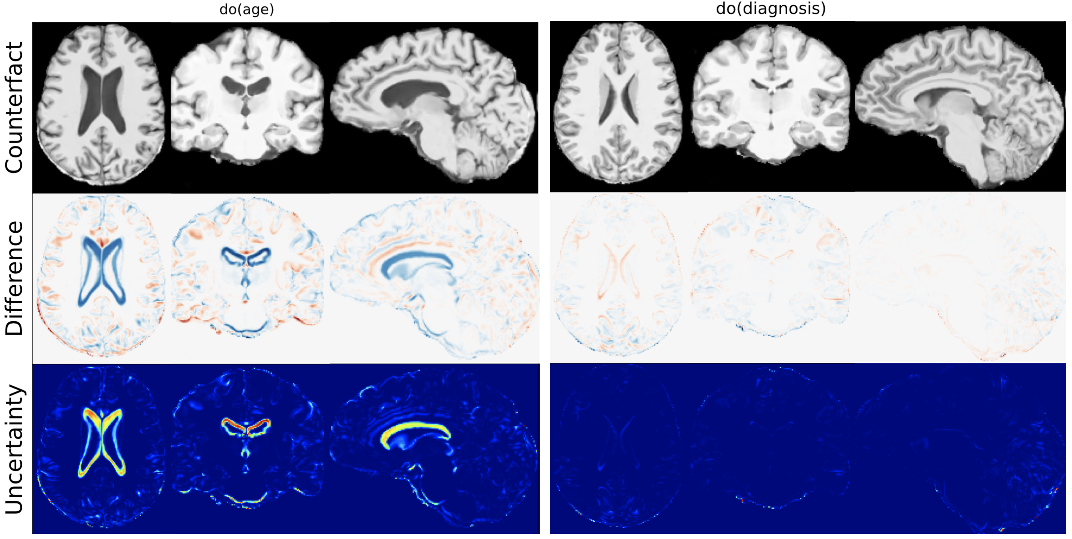
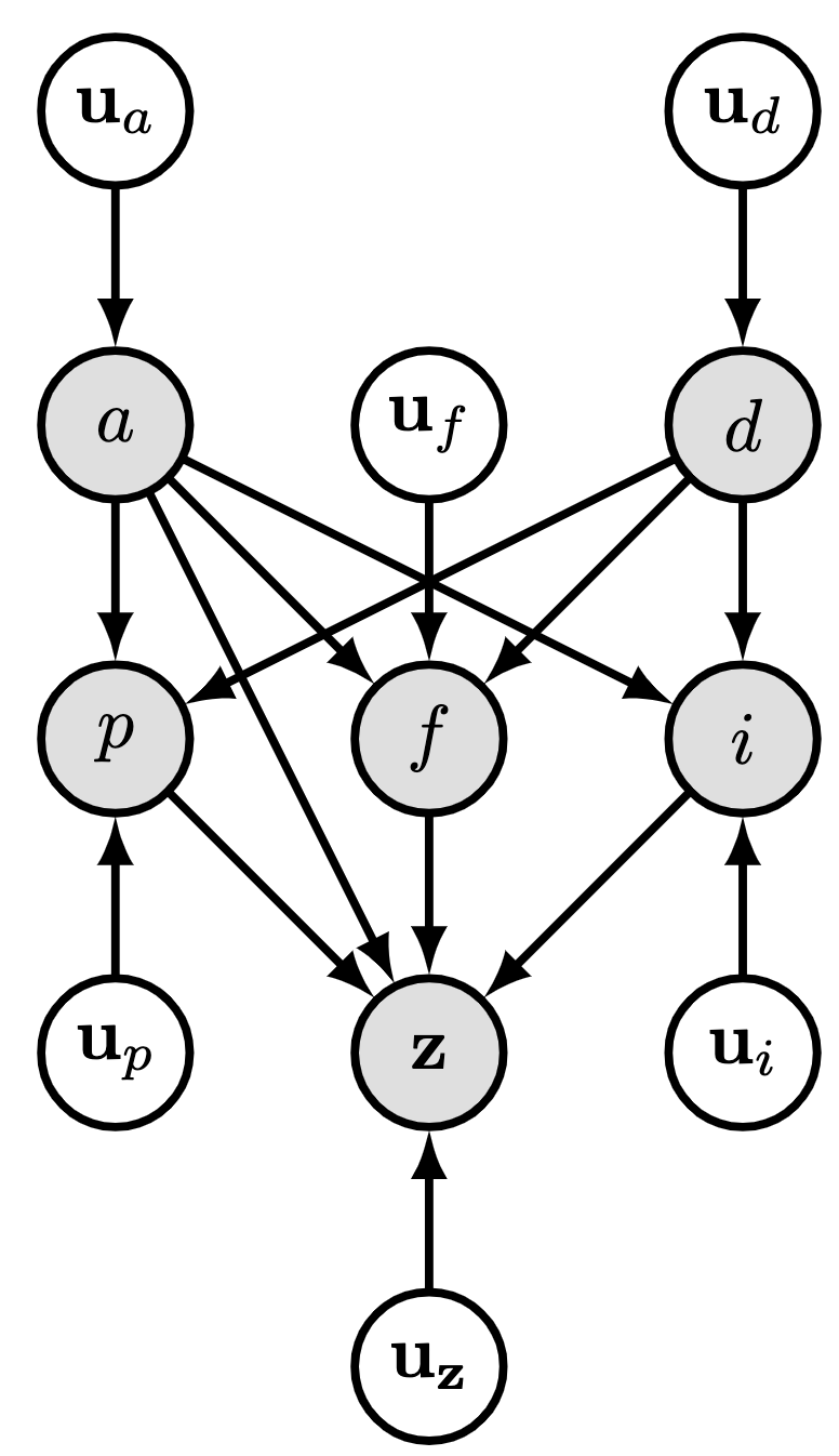
Figure 2: Counterfactual cases. Left: the counterfactual, the differences with original input, and the uncertainty for each intervention. Right: The assumed causal graph is based on [25]. Variables in the graph are: age $(a)$, diagnosis $(d)$, Parietal $(p)$, Frontal $(f)$, Insula $(i)$, and latent features of MRI $(\mathbf{z})$.

This part demonstrates that our model can perform different interventions to the generation process and output high-fidelity 3D counterfactuals. Given a MRI example, we apply an intervention $do()$ to age and diagnosis in our causal graph and generate the 3D counterfactual accordingly. As shown in Fig. 2, we show MRI counterfactual from different views. Our model demonstrates a strong counterfactual generation ability with high fidelity. The diagnosis intervention shows a global but subtle changes on the brain. For the age intervention, we can see clear changes in the Ventricle, a region known to be significantly influenced by the aging process.

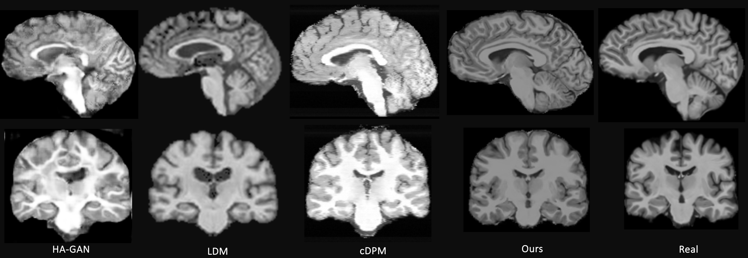
Figure 3: Show cases. 2 views of real MRI vs synthetic MRIs generated by 4 models. Our model can produce visually similar MRI to others but we can do counterfactual generation.

3.2 Counterfactual Evaluation

By preforming random intervention, 400 counterfactuals are synthesized. We then compare with synthetic MRIs from recent generative models and also evaluate it anatomical plausibility to qualify its value for neuroimaging studies. The comparison methods include GAN models like CCE-GAN [30], VAE-GAN [12], $\alpha$-WGAN [10], and HA-GAN [26]; and diffusion models like latent diffusion model (LDM) [21] and cDPM [18]. Qualitative results of all 7 models are shown in Appendix while only the best four are shown in Fig. 3 due to space limitations. Of those four methods, HA-GAN was the only method that was not able to produced the MRIs that looked like those of healthy controls. On the other side LDM produces the noisiest MRI and the MRI of cDPM has clear slice artefacts. In contrast, the MRI of our model shows clear gray-matter boundaries and looks most similar to the real MRI. Finally, our model is much faster than the diffusion-based method as their is no need for the multi-step diffusion process.

We evaluate its anatomical plausibility by comparing its subcortical similarity with the real data. To this end, we run Freesurfer pipeline [5] for both of the 400 real samples and the synthetic ones to conduct the brain pacellation and compute automatic segmentation volume (aseg). We report the effect size (using Cohen’s d coefficient [2], $d$) to 24 sub-cortical differences with the real brain MRIs. As shown in Table 1, 50% of the sub-corticals have a $|d|<0.2$, which means these brain regions are very similar to the real ones. More than 90% of the 24 brain regions have an effect size that is less than 0.4, which suggests that the observed difference between the real and synthetic is relatively minor or subtle.

Table 1: Subcortical Measurement. Cohen’s d is reported here as the effect size (Effect). Most of the ROIs show strong correlations with the real data as they have a small value.

ROI	vessel volume	5th ventricle	optic chiasm	accumbens area	choroid plexus	cc_mid posterior	cc central	cc_mid anterior
Effect	0.0065	-0.0547	-0.4014	-0.0028	0.2400	0.2540	-0.3216	-0.1132
ROI	cc anterior	cc posterior	3rd ventricle	amygdala	4th ventricle	pallidum	WM hypo.	caudate
Effect	0.3581	0.3939	-0.1804	-0.1686	-0.3383	0.5588	-0.0417	-0.1362
ROI	hippo campus	putamen	ventraldc	thalamus	lateral ventricle	brain stem	cerebellum WM	cerebellum cortex
Effect	0.2833	-0.1373	0.6070	0.3978	0.1306	0.2529	0.1690	-0.0748

4 Discussion

While our work proposes novel methodology for embedding counterfactual reasoning into generative AI models to enhance interpretability and generative performance, and outperforms state-of-the-art models in generating 3D MRIs, several challenges remain. Firstly, building a DSCM is challenging on high-dimensional data [3] without sacrificing the quality of generated counterfactuals. This can be further hindered if the size of the dataset is small. To mitigate this issue as much as possible, we compute counterfactuals in the lower-dimensional latent space, although this requires us to control information at a scalar-level, challenging the decoder to generate high-dimensional 3D MRIs.

Secondly, for disease prevention purposes in a clinical setting, it is non-trivial to comprehensively assess the anatomical plausibility of the counterfactuals and generated MRIs when we intervene on a diagnosis, as these present novel findings.

5 Conclusion

We propose a novel brain counterfactual for 3D MRI generation, which fully fills three rungs of Pearl’s ladder of causation. The model adeptly performs causal modeling while capable of generating high-quality 3D brain volumes. This is achieved by our latent structural counterfactual model, which contains a deep SCM constructed in a latent space. We then run a GLM on this low dimensional latent space to synthesize counterfactuals, to mitigate significant computational challenges posed by performing interventions directly on the 3D brain MRIs. The generated MRIs show high anatomical resolution, while the counterfactual generation contains an efficient intervention strategy to generate high-quality 3D counterfactuals.

6 Acknowledgement

Collection and distribution of the NCANDA data were supported by NIH funding AA021681, AA021690, AA021691, AA021692, AA021695, AA021696, AA021697. Access to NCANDA data is available via the NIAAA Data Archive, collection 4513 (https://nda.nih.gov/edit_collection.html?id=4513).

This work was partly supported by funding from the National Institute of Health (MH113406, DA057567, AG084471, AA021697, AA017347, AA010723, AA005965, and AA028840), the DGIST R&D program of the Ministry of Science and ICT of KOREA (22-KUJoint-02), Stanford School of Medicine Department of Psychiatry and Behavioral Sciences Faculty Development and Leadership Award, the Stanford HAI-Google Research Collaboration, the Stanford HAI Google Cloud Credits, the 2024 Stanford HAI Hoffman-Yee Grant, and the UK’s Engineering and Physical Sciences Research Council (EPSRC) Hub for Causality in Healthcare AI (grant number EP/Y028856/1).

References

- [1] Brown, S.A., Brumback, T., Tomlinson, K., Cummins, K., Thompson, W.K., Nagel, B.J., De Bellis, M.D., Hooper, S.R., Clark, D.B., Chung, T., Hasler, B.P., Colrain, I.M., Baker, F.C., Prouty, D., Pfefferbaum, A., Sullivan, E.V., Pohl, K.M., Rohlfing, T., Nichols, B.N., Chu, W., Tapert, S.F.: The National Consortium on Alcohol and Neurodevelopment in Adolescence (NCANDA): a multisite study of adolescent development and substance use. Journal of Studies on Alcohol and Drugs 76(6), 895–908 (2015)
- [2] Cohen, J.: Statistical power analysis for the behavioral sciences. Academic press (2013)
- [3] De Sousa Ribeiro, F., Xia, T., Monteiro, M., Pawlowski, N., Glocker, B.: High fidelity image counterfactuals with probabilistic causal models. In: Proceedings of the 40th International Conference on Machine Learning. Proceedings of Machine Learning Research, vol. 202, pp. 7390–7425 (23–29 Jul 2023), https://proceedings.mlr.press/v202/de-sousa-ribeiro23a.html
- [4] De Sousa Ribeiro, F., Xia, T., Monteiro, M., Pawlowski, N., Glocker, B.: High fidelity image counterfactuals with probabilistic causal models. ICML (2023)
- [5] Fischl, B.: Freesurfer. NeuroImage 62(2), 774–781 (2012)
- [6] Ho, J., Jain, A., Abbeel, P.: Denoising diffusion probabilistic models. Advances in Neural Information Processing Systems 33, 6840–6851 (2020)
- [7] Jung, E., Luna, M., Park, S.H.: Conditional GAN with an attention-based generator and a 3D discriminator for 3D medical image generation. In: Medical Image Computing and Computer-Assisted Intervention, Lecture Notes in Computer Science. vol. 12906, pp. 318–328 (2021)
- [8] Jung, E., Luna, M., Park, S.H.: Conditional GAN with 3D discriminator for MRI generation of Alzheimer’s disease progression. Pattern Recognition 133, 109061 (2023)
- [9] Karras, T., Laine, S., Aila, T.: A style-based generator architecture for generative adversarial networks. In: IEEE/CVF Conference on Computer Vision and Pattern Recognition. pp. 4401–4410 (2019)
- [10] Kwon, G., Han, C., Kim, D.s.: Generation of 3D brain MRI using auto-encoding generative adversarial networks. In: Medical Image Computing and Computer-Assisted Intervention, Lecture Notes in Computer Science. vol. 11766, pp. 118–126 (2019)
- [11] La Barbera, G., Boussaid, H., Maso, F., Sarnacki, S., Rouet, L., Gori, P., Bloch, I.: Anatomically constrained CT image translation for heterogeneous blood vessel segmentation. In: British Machine Vision Virtual Conference. p. 776 (2022)
- [12] Larsen, A.B.L., Sønderby, S.K., Larochelle, H., Winther, O.: Autoencoding beyond pixels using a learned similarity metric. In: International Conference on Machine Learning. pp. 1558–1566. Proceedings of Machine Learning Research (2016)
- [13] Lu, M., Zhao, Q., Zhang, J., Pohl, K.M., Fei-Fei, L., Niebles, J.C., Adeli, E.: Metadata normalization. In: IEEE/CVF Conference on Computer Vision and Pattern Recognition. pp. 10917–10927 (2021)
- [14] van den Oord, A., Vinyals, O., Kavukcuoglu, K.: Neural discrete representation learning. In: Advances in Neural Information Processing Systems. pp. 6309–6318 (2017)
- [15] Pawlowski, N., Coelho de Castro, D., Glocker, B.: Deep structural causal models for tractable counterfactual inference. In: Advances in Neural Information Processing Systems. vol. 33, pp. 857–869 (2020)
- [16] Pawlowski, N., Coelho de Castro, D., Glocker, B.: Deep structural causal models for tractable counterfactual inference. Advances in Neural Information Processing Systems 33, 857–869 (2020)
- [17] Pearl, J.: Causality. Cambridge university press (2009)
- [18] Peng, W., Adeli, E., Bosschieter, T., Park, S.H., Zhao, Q., Pohl, K.M.: Generating realistic brain mris via a conditional diffusion probabilistic model. In: International Conference on Medical Image Computing and Computer-Assisted Intervention. vol. 14227, pp. 14–24. Springer (2023)
- [19] Peters, J., Janzing, D., Schölkopf, B.: Elements of causal inference: foundations and learning algorithms. The MIT Press (2017)
- [20] Petersen, R.C., Aisen, P.S., Beckett, L.A., Donohue, M.C., Gamst, A.C., Harvey, D.J., Jack, C.R., Jagust, W.J., Shaw, L.M., Toga, A.W., Trojanowski, J., Weiner, M.: Alzheimer’s Disease Neuroimaging Initiative (ADNI): clinical characterization. Neurology 74(3), 201–209 (2010)
- [21] Pinaya, W.H., Graham, M.S., Kerfoot, E., Tudosiu, P.D., Dafflon, J., Fernandez, V., Sanchez, P., Wolleb, J., da Costa, P.F., Patel, A., et al.: Generative ai for medical imaging: extending the monai framework. arXiv preprint arXiv:2307.15208 (2023)
- [22] Pinaya, W.H., Tudosiu, P.D., Dafflon, J., Da Costa, P.F., Fernandez, V., Nachev, P., Ourselin, S., Cardoso, M.J.: Brain imaging generation with latent diffusion models. In: Deep Generative Models, Lecture Notes in Computer Science. vol. 13609, pp. 117–126 (2022)
- [23] Rezende, D., Mohamed, S.: Variational inference with normalizing flows. In: International Conference on Machine Learning. pp. 1530–1538. Proceedings of Machine Learning Research (2015)
- [24] Sohl-Dickstein, J., Weiss, E., Maheswaranathan, N., Ganguli, S.: Deep unsupervised learning using nonequilibrium thermodynamics. In: International Conference on Machine Learning. pp. 2256–2265 (2015)
- [25] Sullivan, E.V., Zahr, N.M., Sassoon, S.A., Thompson, W.K., Kwon, D., Pohl, K.M., Pfefferbaum, A.: The role of aging, drug dependence, and hepatitis c comorbidity in alcoholism cortical compromise. Jama Psychiatry 75(5), 474–483 (2018)
- [26] Sun, L., Chen, J., Xu, Y., Gong, M., Yu, K., Batmanghelich, K.: Hierarchical amortized GAN for 3D high resolution medical image synthesis. IEEE Journal of Biomedical and Health Informatics 26(8), 3966–3975 (2022)
- [27] Tabak, E.G., Vanden-Eijnden, E.: Density estimation by dual ascent of the log-likelihood. Communications in Mathematical Sciences 8(1), 217–233 (2010)
- [28] Wolleb, J., Bieder, F., Sandkühler, R., Cattin, P.C.: Diffusion models for medical anomaly detection. In: Medical Image Computing and Computer-Assisted Intervention, Lecture Notes in Computer Science. vol. 13438, pp. 35–45 (2022)
- [29] Xia, K.M., Pan, Y., Bareinboim, E.: Neural causal models for counterfactual identification and estimation. In: The Eleventh International Conference on Learning Representations (2023), https://openreview.net/forum?id=vouQcZS8KfW
- [30] Xing, S., Sinha, H., Hwang, S.J.: Cycle consistent embedding of 3D brains with auto-encoding generative adversarial networks. In: Medical Imaging with Deep Learning (2021)
- [31] Zhao, Q., Liu, Z., Adeli, E., Pohl, K.M.: Longitudinal self-supervised learning. Medical Image Analysis 71, 102051 (2021)
- [32] Zheng, S., Charoenphakdee, N.: Diffusion models for missing value imputation in tabular data. In: NeurIPS Table Representation Learning (TRL) Workshop (2022)