Compartmental and Coexistence in the Dark Sector of the Universe

Abstract

We revise the cosmological interaction between dark energy and dark matter. More precisely, we focus on models that support compartmentalization or co-existence in the dark sector of the universe. Within the framework of a homogeneous and isotropic, spatially flat Friedmann–Lemaître–Robertson–Walker geometry, we analyse the asymptotic behaviour of the physical parameters for two interacting models, where dark energy and dark matter have constant equations of state parameters, in the presence of dark radiation, when dark energy is described by a quintessence scalar field. For each model, we determine the asymptotic solutions and attempt to understand how the interaction affects the cosmological evolution and history.

I Introduction

The nature of dark energy and dark matter is a mystery. These exotic fluids do not interact with light, and we observe only the gravitational effects they are responsible for; they form the so-called dark sector of the universe. Dark matter has been introduced to explain the velocity profile of galaxies dm1 . On the other hand, dark energy de1 has been introduced to explain cosmic acceleration rr1 ; Kowal . In contrast to dark matter, which exerts gravitational effects, dark energy exerts repulsive forces that lead to anti-gravitational effects. In gravitational physics, matter sources are described by the formalism of fluid dynamics.

On large scales, where the universe is isotropic and homogeneous, as described by the Friedmann–Lemaître–Robertson–Walker (FLRW) geometry, dark matter is described by a pressureless fluid source, also known as dust, while dark energy is described by a perfect fluid with a negative equation of state parameter de1 .

The cosmological constant provides the simplest mechanism for describing dark energy rr1 . Despite the fact that the cosmological constant introduces the fewest degrees of freedom and is in agreement with the majority of cosmological data, it suffers from various problems. For a recent discussion on the challenges of the cosmological constant, we refer the reader to lpe1 . In order to overcome the puzzles of the cosmological constant, cosmologists have dealt with the introduction of other dark energy models with a dynamical equation for the state parameter. The origin of the new dynamical variables is mainly attributed to the existence of scalar fields nik ; gal02 ; hor ; in01 ; in02 ; in03 ; in06 ; in07 , or to modifications of the gravitational action integral mod0 ; mod00 ; mod7 ; Ferraro ; Ferraro2 ; in08 ; on2 ; Clifton ; revh .

Interaction in the dark sector of the universe Amendola:1999er , that is, energy transfer between dark matter and dark energy has been proposed as a potential mechanism to explain the cosmic coincidence problem con1 ; con2 ; con3 ; con4 . Indeed, the existence of this interaction leads to new dynamical behaviour of the physical variables. Because of an interaction it is possible the nature of the dark energy fluid can change. Although the interaction between dark energy and dark matter is mainly a phenomenological consideration, there are various theoretical models that predict an interaction, such as a Weyl integrable spacetime salim ; ww01 , the Chameleon mechanism ch1 ; am1 , a conformal transformation sf3 ; sf4 , Chiral scalar fields qq2 ; ancqg ; atr6 ; vr91 and others. The analysis of the cosmological observations with the interacting models has shown that the existence of a nonzero energy transfer term between these two fluids can be a potential solutions for the cosmological tensions, that is, the $H_{0}$ tensions and the $\sigma_{8}$ tension Kumar:2017dnp ; DiValentino:2017iww ; span ; Kumar:2019wfs ; Pourtsidou:2016ico ; An:2017crg ; luca1 ; poi . There is a plethora of interacting models which have been proposed in the literature, see for instance ss1 ; ss2 ; ss3 ; ss4 ; ss5 ; ss6 ; ss7 ; ss8 ; ss9 ; ss10 ; ss11 ; ss12 ; ss14 ; ss15 ; ss16 ; ss17 ; qq and references therein.

In biological systems, understanding dynamic interactions and predicting future states can be quite complex due to the multitude of interacting components and variables. Compartmental models serve as a powerful tool in simplifying these complexities by segregating a biological system into interconnected, homogeneous compartments representing different states or classes of elements within the system. Compartmental models can provide detailed quantitative analyses by defining transfer rates between compartments, which is crucial for understanding system dynamics and predicting future states, especially useful in epidemiology. These models also allow for robust parameter estimation and can be adapted or generalized for various studies. Additionally, they integrate data from multiple sources, enhancing analysis accuracy and robustness across fields like ecology and epidemiology. A similar approach is used in this study, where dark matter and dark energy are considered as compartments of variable composition. An additional term in the energy conservation equations represents the energy exchange between these compartments. Analyses of the differential equations of the system are used to explore the long-term behavior of the universe, using techniques to simplify the equations.

In this study, we employ dynamical system analysis to investigate the evolution of the physical parameters for some dark energy and dark matter interacting models which describe compartmentalization or coexistence in the dark sector of the universe. The analysis of phase space is a powerful method for studying the asymptotic behaviour of a given cosmological model, as well as for the reconstruction of the provided cosmological history dyn1 ; dyn2 ; dyn3 ; dyn4 ; dyn5 ; dyn6 ; dyn7 ; dyn8 ; dyn9 ; dyn10 . The method has been widely applied in the analysis of background equations in model cosmology, as well as in the analysis of the asymptotic behaviour of cosmological perturbations dp1 ; dp2 . The structure of the paper is as follows.

In Section II, we introduce the cosmological model under our consideration, which is that of an isotropic and homogeneous spatially flat FLRW geometry. Moreover, the continuity equation for the cosmological fluid is discussed, and the concept of interaction is introduced. In Section III, we assume that the cosmological fluid consists of dark energy and dark matter. These two fluids are assumed to have constant equation-of-state parameters, but they have a nonzero interaction term. We consider two interacting functions which can describe compartmentalization or co-existence between the two fluids in the dark sector of the universe. We employ the $H$-normalization approach and perform a detailed analysis of the solution space for the field equations. In particular, we calculate the stationary points and determine their stability properties, as well as the physical properties of the asymptotic solutions.

In order to make our analysis more practical, in Section IV, we introduce a radiation term. The existence of radiation leads to a new behaviour in the evolution of the dynamics. Moreover, in Section V, we replace the minimally coupled radiation fluid with that of dark radiation. This is an exotic matter source which interacts with the other two fluids of the dark sector of the universe. In Section VI, we assume that the dark energy fluid is described by a scalar field minimally coupled to gravity. In this framework, dark energy has a dynamical equation of state parameter. We focus only on the case where dark matter exists and investigate the solution space. Because of the new dynamical variables introduced by the scalar field, the evolution of the physical solutions differs from those found before. Finally, in Section VII, we summarize the results and draw our conclusions.

II The Cosmological model

According to the cosmological principle, the geometry which describes the universe on large scales is the spatially flat FLRW metric with line element

$$ds^{2}=-dt^{2}+a^{2}(t)\left(dx^{2}+dy^{2}+dz^{2}\right)\;.$$ (1)

Function $a(t)$ describes the radius of a three-dimensional space, and the expansion is given by the Hubble function $H=\frac{\dot{a}}{a}$, $\dot{a}=\frac{da}{dt}$. The line element (1) is isotropic and homogeneous where from the Einstein tensor

$$G_{\mu\nu}\equiv R_{\mu\nu}-\frac{R}{2}g_{\mu\nu}\;,$$ (2)

only the diagonal terms survive

$$G_{\mu\nu}=diag\left(3H^{2},-2\dot{H}-3H^{2},-2\dot{H}-3H^{2},-2\dot{H}-3H^{2}\right)\;.$$ (3)

The gravitational field equations of Einstein’s General Relativity are

$$G_{\mu\nu}=T_{\mu\nu},$$ (4)

where $T_{\mu\nu}$ is the energy momentum tensor which attributes the matter source in the universe.

For the FLRW geometry, and for the Einstein tensor (3) it is obvious that $T_{\mu\nu}$ inherits the properties of $G_{\mu\nu}$; consequently, the cosmological fluid is describe by an isotropic and homogeneous perfect fluid, i.e.

$$T_{\mu\nu}=\left(\rho+p\right)u_{\mu}u_{\nu}+pg_{\mu\nu}\;,$$ (5)

where $u^{\mu}$ is the comoving observer, $u^{\mu}=\delta_{t}^{\mu}$, $\rho\left(t\right)$ is the energy density and $p\left(t\right)$ is the pressure component. Hence, the field equations are

$$3H^{2} = \rho\;,$$ (6)

$$2\dot{H}+3H^{2} = -p\;.$$ (7)

The Bianchi identity gives $G_{~{}~{}~{};\nu}^{\mu\nu}=0$, from where we calculate the equation of motion for the cosmological fluid

$$T_{~{}~{};\nu}^{\mu\nu}=0\;,$$ (8)

or for the FLRW geometry

$$\dot{\rho}+3H\left(\rho+p\right)=0\;.$$ (9)

The effective equation of state parameter for the cosmological fluid is defined as $w_{eff}=\frac{p}{\rho}$. With the application of the field equations the latter parameter is expressed as

$$w_{eff}=-1-\frac{2}{3}\frac{\dot{H}}{H^{2}}.$$ (10)

II.1 The Dark Sector of the Universe

Using the latest cosmological observations, the universe is dominated by two fluid sources known as dark matter and dark energy. These two fluids do not absorb or radiate light and are detected only through the gravitational phenomena related to them. In the period of galaxy formation, dark matter dominated the universe, while today dark energy dominates.

The energy momentum tensor is defined as

$$T_{\mu\nu}=T_{\mu\nu}^{m}+T_{\mu\nu}^{DE}.$$ (11)

Dark matter is the “missing” matter source in galaxy formation, whose gravitational effect can explain the velocity profile for the stars in galaxies. At cosmological scales the pressure component is neglected, that is,

$$T_{\mu\nu}^{m}=\rho_{m}u_{\mu}u_{\nu}.$$ (12)

On the other hand, dark energy is responsible for the late-time rapid expansion of the universe. It has a negative pressure component, which is related to anti-gravitational forces. The energy-momentum tensor associated with dark energy is

$$T_{\mu\nu}^{DE}=\left(\rho_{d}+p_{d}\right)u_{\mu}u_{\nu}+p_{d}g_{\mu\nu},~{}$$ (13)

from where we can define the equation of state parameter $w_{d}=\frac{p_{d}}{\rho_{d}}$. In the following, we consider $w_{d}<0$. By replacing (11) in (8) we find

$$\left(T_{\mu\nu}^{m}g^{\nu\kappa}+T_{\mu\nu}^{DE}g^{\nu\kappa}\right)_{;\kappa}=0\;,$$ (14)

which, equivalently, can be expressed as

$$\left(T_{\mu\nu}^{m}g^{\nu\kappa}\right)_{;\kappa}=Q~{},~{}\left(T_{\mu\nu}^{DE}g^{\nu\kappa}\right)_{;\kappa}=-Q.$$ (15)

Here, the interaction function $Q\left(t\right)$ describes the energy transfer between the two fluids. Thus from (15) in terms of coordinates it follows

$$\dot{\rho}_{m}+3H\rho_{m} = Q,$$ (16)

$$\dot{\rho}_{d}+3H\left(\rho_{d}+p_{d}\right) = -Q.$$ (17)

When the fluids are minimally coupled to each other, $Q\left(t\right)=0$, and from (15) we find the two conservation equations

$$\dot{\rho}_{m}+3H\rho_{m} = 0,$$ (18)

$$\dot{\rho}_{d}+3H\left(\rho_{d}+p_{d}\right) = 0.$$ (19)

Nevertheless, it is possible for the two fluids to interact and the function $Q\left(t\right)$ to be nonzero, i.e. $Q\left(t\right)\neq 0$. In this case there exists energy transfer between the two fluids.  For $Q\left(t\right)>0$, there is mass transfer from dark energy to dark matter, while for $Q\left(t\right)<0$ dark matter is converted into dark energy.

A nonzero interaction component in the dark sector of the universe is not neglected by the cosmological data. There are studies which support the existence of mass transfer spp1 ; spp2 . Although there are theoretical models where dark energy and dark matter are two different contributions in a universe of a generic fluid source.

III Dark Matter - Dark Energy

In this piece of study, we follow a phenomenological approach and consider an interacting function such that the two fluids to be described by the simplest model of “competitive fluids”, a Lotka-Volterra type system, or a compartmental model such as the SIR model.

III.1 The Compartmental Interaction

From the interacting function mag ; kos

$$Q_{A}\left(t\right)=Q_{0}\left(t\right)\rho_{m}\rho_{d},$$ (20)

introduced in qq , equations (15) become

$$\dot{\rho}_{m}+3H\rho_{m} = Q_{0}\left(t\right)\rho_{m}\rho_{d},$$ (21)

$$\dot{\rho}_{d}+3H\left(\rho_{d}+p_{d}\right) = -Q_{0}\left(t\right)\rho_{m}\rho_{d},$$ (22)

where $Q_{0}\left(t\right)$ has dimensions of $H^{-1}$. The latter system can be expressed as

$$\dot{\rho}_{m}+3H\rho_{m} = Q_{0}\left(t\right)\rho_{m}\rho_{d},$$ (23)

$$\dot{\rho}_{d}+3\left(1+w_{d}\right)H\rho_{d} = -Q_{0}\left(t\right)\rho_{m}\rho_{d}.$$ (24)

This interaction model does not suffer from early instabilities kos .

Although the aforementioned system has the form of the Lotka-Volterra system with non-constant coefficients, the Hubble function $H\left(t\right)$ is related to the energy densities $\rho_{m}$, $\rho_{d}$, from the Friedmann equation (6), that is, $3H^{2}=\rho_{m}+\rho_{d}$. Consequently, the dynamical system (23), (24) is a type of compartmental model. These models are mainly applied in epidemiology and are known as SIR models.

III.1.1 Asymptotic analysis

We introduce $Q_{0}\left(t\right)=\frac{\alpha}{H}$, where $\alpha$ is a constant, and the dimensionless variables

$$\Omega_{m}=\frac{\rho_{m}}{3H^{2}}~{},~{}\Omega_{DE}=\frac{\rho_{d}}{3H^{2}}~{},~{}\tau=\ln a.$$ (25)

Recall that the dimensionless variables have the constraint $\left\{\Omega_{m},\Omega_{DE}\right\}\in\left[0,1\right]$.

Hence, equations (23), (24) read

$$\frac{d\Omega_{m}}{d\tau} = 3\left(\alpha+w_{d}\right)\Omega_{m}\Omega_{DE},$$ (26)

$$\frac{d\Omega_{DE}}{d\tau} = 3\Omega_{DE}\left(w_{d}\left(\Omega_{DE}-1\right)-\alpha\Omega_{m}\right).$$ (27)

We remark that in terms of the dimensionless variables, where the Hubble function has been eliminated by the dynamical system, it is clear that this model is a compartmental model.

Furthermore, from the Friedmann’s equation (6) it follows

$$\Omega_{m}+\Omega_{DE}=1.$$ (28)

With the use of the latter constraint we can reduce by one the dimension of the dynamical system (26), (27).

Hence the final equation is

$$\frac{d\Omega_{DE}}{d\tau}=3\left(\alpha+w_{d}\right)\Omega_{DE}\left(\Omega_{DE}-1\right)\;.$$ (29)

Stationary points

We assume that $w_{d}$ is a constant, and then we calculate the stationary points. For $\alpha+w_{d}\neq 0$, there exist two stationary points, point $P_{1}$ with $\Omega_{DE}\left(P_{1}\right)=0$ and $P_{2}$ with $\Omega_{DE}\left(P_{2}\right)=1$.

The point $P_{1}$ describes an asymptotic solution where dark matter dominates in the universe, and the effective cosmological fluid has the equation of state parameter $w_{eff}\left(P_{1}\right)=0$. The stationary point is an attractor for $\left(\alpha+w_{d}\right)>0$.

On the other hand, point $P_{2}$ corresponds to an asymptotic solution where the dark energy dominates, that is, $w_{eff}\left(P_{2}\right)=w_{d}$. Last but not least, $P_{2}$ is an attractor when $\left(\alpha+w_{d}\right)<0$.

III.1.2 Analytic solution

The nonlinear differential equation (29) can be solved analytically. Indeed, the solution in terms of the scale factor $\tau=\ln a$ is given as follows:

$$\Omega_{DE}\left(a\right)=\left[1+\Omega^{0}a^{3\left(\alpha+w_{d}\right)}\right]^{-1}\;,$$ (30)

from which we construct the Hubble function

$$H\left(a\right)=\hat{H}_{0}\left[1+\Omega^{0}a^{3\left(\alpha+w_{d}\right)}\right]^{\frac{w_{d}}{2\left(w_{d}+\alpha\right)}}\left[\Omega^{0}a^{3\left(\alpha+w_{d}\right)}\left(\alpha+w_{d}\right)\right]^{-\frac{1+w_{d}}{2\left(\alpha+w_{d}\right)}}\;.$$ (31)

Here $\Omega^{0}$ and $\hat{H}_{0}$ are integration constants. If $w_{d}=-1$, the latter analytic expression for the scale factor becomes

$$H\left(a\right)=\hat{H}_{0}\left(1+\Omega^{0}a^{3\left(\alpha-1\right)}\right)^{-\frac{1}{2\left(\alpha-1\right)}}.$$ (32)

For $\alpha=0$, we recover the $\Lambda$CDM universe, that is,

$$H\left(a\right)=H_{0}\left(\Omega_{\Lambda}^{0}+\Omega_{m}^{0}a^{-3}\right)^{\frac{1}{2}},$$ (33)

where we have replaced $\hat{H}_{0}=H_{0}(\Omega_{\Lambda}^{0})^{\frac{1}{2}}$, and $\Omega_{m}=\Omega_{\Lambda}^{0}\Omega^{0}$.

III.2 The Lotka-Volterra Interaction

The Lotka-Volterra model describes co-existence. In order to recover such behaviour between the dark energy and the dark matter we introduce the interaction yc1

$$Q_{B}\left(t\right)=Q_{0}\left(t\right)\rho_{m}\rho_{d}+Q_{1}\left(t\right)\rho_{d},$$ (34)

where $Q_{0}\left(t\right)$ has the dimensions of $H^{-1}$ and $Q_{1}\left(t\right)$ has the dimensions of $H$.

For this interaction the continuous equations for the two fluids reads

$$\dot{\rho}_{m}+3H\rho_{m} = Q_{0}\left(t\right)\rho_{m}\rho_{d}+Q_{1}\left(t\right)\rho_{d}.$$ (35)

$$\dot{\rho}_{d}+3\left(1+w_{d}\right)H\rho_{d} = -Q_{0}\left(t\right)\rho_{m}\rho_{d}-Q_{1}\left(t\right)\rho_{d}.$$ (36)

We proceed with an asymptotic analysis of the field equations for this interacting model, where we assume that $Q_{0}\left(t\right)=\frac{\alpha}{H}$ and $Q_{1}\left(t\right)=\beta H$, with $\alpha$,$~{}\beta$ constant parameters.

III.2.1 Asymptotic analysis

We apply the same algorithm as before and introduce dimensionless variables (25). The field equations with dimensionless variables form the dynamical system

$$\frac{d\Omega_{m}}{d\tau} = 3\left(\alpha+w_{d}\right)\Omega_{m}\Omega_{DE}+\beta\Omega_{DE},$$ (37)

$$\frac{d\Omega_{DE}}{d\tau} = 3\Omega_{DE}\left(w_{d}\left(\Omega_{DE}-1\right)-\alpha\Omega_{m}\right)-\beta\Omega_{DE},$$ (38)

with constraint equation (28).

Applying the constraint (28) results in the single differential equation

$$\frac{d\Omega_{DE}}{d\tau}=\left(3\left(\alpha+w_{d}\right)\left(\Omega_{DE}-1\right)-\beta\right)\Omega_{DE}\text{.}$$ (39)

Stationary points

The stationary points of equation (39) are the two points $\bar{P}_{1}$ with $\Omega_{DE}\left(\bar{P}_{1}\right)=0$ and $\bar{P}_{2}$ with $\Omega_{DE}\left(\bar{P}_{2}\right)=1+\frac{\beta}{3\left(\alpha+w_{d}\right)}$.

The point $\bar{P}_{1}$ describes a universe dominated by dark matter, that is, $\Omega_{m}\left(\bar{P}_{1}\right)=1$. On the other hand, point $\bar{P}_{2}$ describes a universe of coexistence between the two fluids. The solution is physically accepted when $0\leq\Omega_{DE}\left(\bar{P}_{2}\right)\leq 1$, that is, $-1\leq\frac{\beta}{3\left(\alpha+w_{d}\right)}\leq 0$. The equation of state parameter for the effective fluid in solution $\bar{P}_{2}$ is derived $w_{eff}\left(\bar{P}_{2}\right)=w_{d}\left(1+\frac{\beta}{3\left(\alpha+w_{d}\right)}\right)$.

As far as the stability of the stationary points is concerned, point $\bar{P}_{1}$ is attractor when $3\left(\alpha+w_{d}\right)+\beta>0$, while $\bar{P}_{2}$ is an attractor when $-3\left(\alpha+w_{d}\right)<\beta\leq 0$.

We obtain similar results for the more general model of the Lotka-Volterra family, $Q\left(t\right)=Q_{0}\left(t\right)\rho_{m}\rho_{d}+Q_{1}\left(t\right)\rho_{m}+Q_{2}\left(t\right)\rho_{d}$. Specifically, for this model we find two stationary points that describe co-existence. When $Q_{1}\left(t\right)$, or $Q_{2}\left(t\right)$ becomes zero, one of the coexistence points reduced to that of $P_{1}$, or $P_{2}$, for the studied before for the compartmental interaction.

Furthermore, when $\alpha=0,~{}\beta=0$, the $\Lambda$CDM universe is recovered for $\hat{H}_{0}=H_{0}\Omega_{\Lambda}$, and $\Omega_{m}=\Omega_{\Lambda}\Omega^{0}$.

III.2.2 Analytic solution

The analytic solution of equation (39) in terms of the scale factor is

$$\Omega_{DE}\left(a\right)=\left(1+\frac{\beta}{3\left(\alpha+w_{d}\right)}\right)\left(1+\Omega^{0}a^{3\left(\alpha+w_{d}\right)+\beta}\right)^{-1},$$ (40)

and the analytic expression for the Hubble function is

$$H\left(a\right)=\hat{H}_{0}\left(1+\Omega^{0}a^{3\left(\alpha+w_{d}\right)+\beta}\right)^{\frac{w_{d}}{2\left(\alpha+w_{d}\right)}}a^{-3\left(1+w_{d}\left(1+\frac{\beta}{3\left(\alpha+w_{d}\right)}\right)\right)}.$$ (41)

Thus, for the case where $w_{d}=-1$, the latter solution becomes

$$H\left(a\right)=\hat{H}_{0}\left(1+\Omega^{0}a^{3\left(\alpha-1\right)+\beta}\right)^{-\frac{1}{2\left(\alpha-1\right)}}a^{\frac{\beta}{\left(\alpha-1\right)}}.$$ (42)

IV Dark Energy - Dark Matter - Radiation

Although the contribution of the radiation in the total cosmological fluid can be neglected nowadays, radiation played an important role in the early stages of the universe. In order to present a more realistic model, we consider the energy tensor for the cosmological model to depend on the three fluids,

$$T_{\mu\nu}=T_{\mu\nu}^{m}+T_{\mu\nu}^{DE}+T_{\mu\nu}^{r}$$ (43)

where $T_{\mu\nu}^{r}$ describes the radiation component defined as

$$T_{\mu\nu}^{r}=\left(\rho_{r}+p_{r}\right)u_{gm}u_{\nu}+p_{r}g_{\mu\nu}~{},~{}p_{r}=\frac{1}{3}\rho_{r}.$$ (44)

The conservation law (14) is modified as

$$\left(T_{\mu\nu}^{m}g^{\nu\kappa}+T_{\mu\nu}^{DE}g^{\nu\kappa}+T_{\mu\nu}^{r}g^{\nu\kappa}\right)_{;\kappa}=0,$$ (45)

where since radiation does not interact with the rest of the dark components of the universe, it follows

$$\left(T_{\mu\nu}^{m}g^{\nu\kappa}+T_{\mu\nu}^{DE}g^{\nu\kappa}\right)_{;\kappa}=0~{},~{}\left(T_{\mu\nu}^{r}g^{\nu\kappa}\right)_{;\kappa}=0,$$ (46)

Consequently, in a FLRW background the continuous equation for the radiation fluid reads

$$\dot{\rho}_{r}+\frac{4}{3}H\rho_{r}=0.$$ (47)

IV.1 The Compartmental Interaction

Let us consider the compartmental interaction $Q\left(t\right)$ as given in expression (20) with $Q_{0}\left(t\right)=\frac{\alpha}{H}$. We introduce the new dimensionless variable $\Omega_{r}=\frac{\rho_{r}}{3H^{2}}$ which describes the energy density for the radiation fluid, and $\Omega_{r}\in\left[0,1\right]$.

IV.1.1 Asymptotic analysis

The cosmological field equations in terms of the dimensionless variables (25) are

$$\frac{d\Omega_{m}}{d\tau} = 3\left(\alpha+w_{d}\right)\Omega_{m}\Omega_{DE}+\Omega_{m}\Omega_{r},$$ (48)

$$\frac{d\Omega_{DE}}{d\tau} = 3\Omega_{DE}\left(w_{d}\left(\Omega_{DE}-1\right)-\alpha\Omega_{m}\right)+\Omega_{DE}\Omega_{r},$$ (49)

where for the first Friedmann’s equation we derive the constraint

$$\Omega_{r}=1-\Omega_{m}-\Omega_{DE}.$$ (50)

We proceed with the analysis of the stationary points for the two-dimensional system (48), (49). For each stationary point, we discuss the physical properties of the asymptotic solution and its stability properties. Indeed, the equation of state parameter for the effective fluid in terms of the dimensionless variables is

$$w_{eff}=w_{d}\Omega_{DE}+\frac{1}{3}\Omega_{r}\text{.}$$ (51)

Stationary points

The dynamical system (48), (49) admits four stationary points $A=\left(\Omega_{m}\left(A\right),\Omega_{DE}\left(A\right)\right)$, with coordinates; $A_{1}=\left(1,0\right)$; $A_{2}=\left(0,1\right)$; $A_{3}=\left(0,0\right)$ and $A_{4}=\left(\frac{1-3w_{d}}{3\alpha},-\frac{1}{3\alpha}\right)$.

The stationary points $A_{1}$ and $A_{2}$ correspond to universes without a radiation component, that is, $\Omega_{r}\left(A_{1,2}\right)=0$. That is, points $A_{1}$, $A_{2}$ have the same physical properties with that of $P_{1}$ and $P_{2}$ found before. We linearize the dynamical system (48), (49) around the stationary points and we calculate the eigenvalues $e_{1}\left(A_{1}\right)=-1$, $e_{2}\left(A_{1}\right)=-3\left(w_{d}+\alpha\right)$ and $e_{1}\left(A_{2}\right)=-1+3w_{d}$, $e_{2}\left(A_{2}\right)=3\left(w_{d}+\alpha\right)$. Thus, the point $A_{1}$ is an attractor for $\alpha>0$ and $-\alpha<w_{d}<0$, while $A_{2}$ is an attractor for $\left\{\alpha<0,w_{d}<0\right\}$, or $\left\{\alpha>0,w_{d}<-\alpha\right\}$.

Concerning the asymptotic solution at point $A_{3}$, it describes a universe dominated by the radiation fluid, that is, $\Omega_{r}\left(A_{3}\right)=0$. The eigenvalues around the stationary point $A_{3}$ are $e_{1}\left(A_{3}\right)=1$, $e_{2}\left(A_{3}\right)=1-3w_{d}$, which means that point $A_{3}$ is always a source.

Finally, point $A_{4}$ describes a universe where all the fluid contributes in the cosmological evolution. However, because we have assumed $w_{d}<0$, it follows that the point is not physically accepted.

Two-dimensional phase-space portraits for the dynamical system (48), (49) are presented in Fig. 1. The portraits are for $w_{d}=-1$ and for two values of the parameter $\alpha$, where point $A_{1}$ or $A_{2}$ are attractors. We remark that for $w_{d}=-1$ point $A_{2}$ describes the de Sitter universe.

Furthermore, in Fig. 2 we present the qualitative evolution for the energy density parameters $\Omega_{m},~{}\Omega_{DE}$ and $\Omega_{r}$, for values of the free parameters such that the future attractor is the point $A_{2}$ and describes the de Sitter solution. Finally, the qualitative evolution of the effective equation of state parameter $w_{eff}$ is given in Fig. 3.

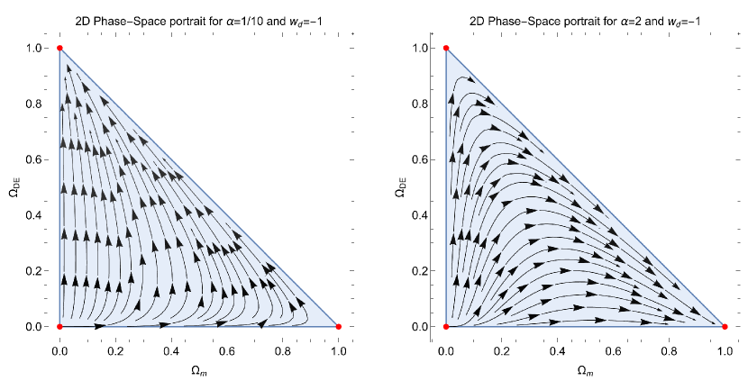
Figure 1: Compartmental: Phase-space portraits for the dynamical system (48), (49) for $w_{d}=-1$ and $\alpha=\frac{1}{10}$ (left fig.) and $\alpha=2$ (right fig.). The physical accepted stationary points are marked with red dots. In the left fig. point $A_{2}$ is an attractor, while in the right fig. the attractor is the stationary point $A_{2}$.

Figure 2: Compartmental: Qualitative evolution of the energy density parameters $\Omega_{m},~{}\Omega_{DE}$ and $\Omega_{r}$, for values of the free parameters such that the future attractor of the dynamical system (48), (49) is the point $A_{2}$ and describe the de Sitter solution.

Figure 3: Compartmental: Qualitative evolution of $w_{eff}$ for values of the free parameters such that the future attractor for the dynamical system (48), (49) is the point $A_{2}$ and the initial conditions are of that of Fig. 2.

IV.2 The Lotka-Volterra Interaction

In this Section, we study the asymptotic behaviour of the field equations for the interaction model (34), which leads to a modified Lotka-Volterra system.

IV.2.1 Asymptotic analysis

For interaction (34) the field equations in terms of the dimensionless variables $\left\{\Omega_{m},\Omega_{DE},\Omega_{r},\tau\right\}$ are expressed as follows

$$\frac{d\Omega_{m}}{d\tau} = 3\left(\alpha+w_{d}\right)\Omega_{m}\Omega_{DE}+\beta\Omega_{DE}+\Omega_{m}\Omega_{r},$$ (52)

$$\frac{d\Omega_{DE}}{d\tau} = 3\Omega_{DE}\left(w_{d}\left(\Omega_{DE}-1\right)-\alpha\Omega_{m}\right)-\beta\Omega_{DE}+\Omega_{DE}\Omega_{r},$$ (53)

with constraint equation (50).

Moreover, the equation of state parameter for the effective cosmological fluid is given by expression (51). In the following section, we investigate the stationary points of this two-dimensional system.

Stationary points

The dynamical system (52), (53) admits the stationary points $\bar{A}=\left(\Omega_{m}\left(\bar{A}\right),\Omega_{DE}\left(\bar{A}\right)\right)$ with coordinates $\bar{A}_{1}=\left(1,0\right)\,\,$; $\bar{A}_{2}=\left(-\frac{\beta}{3\left(\alpha+w_{d}\right)},1+\frac{\beta}{3\left(\alpha+w_{d}\right)}\right)$; $\bar{A}_{3}=\left(0,0\right)$ and $\bar{A}_{4}=\left(\frac{1-3w_{d}+\beta}{\alpha},-\frac{1}{3\alpha}+\frac{\beta}{3\alpha\left(1-3w_{d}\right)}\right)$.

The points $\bar{A}_{1}$, $\bar{A}_{2}$ describe solutions without radiation, i.e. $\Omega_{r}\left(\bar{A}_{1,2}\right)=0$. Hence, asymptotic solutions have similar properties as those described by points $\bar{P}_{1}$ and $\bar{P}_{2}$ respectively. Furthermore, the point $\bar{A}_{3}$ describes a universe dominated by the radiation fluid. Finally, point $\bar{A}_{4}$ is physically accepted for $w_{d}=\frac{1-\beta}{3}$, with $\beta>1$ and $\alpha\neq 0$. However, in this case, the point $\bar{A}_{4}$ is identical to $\bar{A}_{3}$ and always describes the radiation solution.

The eigenvalues of the two-dimensional linearized system (52), (53) around the stationary points $\bar{A}_{1}$ and $\bar{A}_{2}$ are $e_{1}\left(\bar{A}_{1}\right)=-1$, $e_{2}\left(\bar{A}_{1}\right)=-\left(3\left(w_{d}+\alpha\right)+\beta\right)$; $e_{1}\left(\bar{A}_{2}\right)=-1+w_{d}\left(3+\frac{\beta}{\alpha+w_{d}}\right)$, $e_{2}\left(\bar{A}_{2}\right)=3\left(w_{d}+\alpha\right)+\beta$. Hence, point $\bar{A}_{1}$ is an attractor for $\alpha>-\frac{\beta}{3}$, $-\frac{3\alpha+\beta}{3}<w_{d}<0$; while point $\bar{A}_{2}$ is an attractor when $a<0$ and $\beta<-3\left(\alpha+w_{d}\right)$ or $\alpha>0$ with constraints $\left\{w_{d}<-\alpha,\beta<-3\left(w_{d}+\alpha\right)\right\}$ or $\left\{-\alpha<w_{d}<0,-\frac{\left(1+w_{d}\right)\left(\alpha+w_{d}\right)}{w_{d}}<\beta<-3\left(\alpha+w_{d}\right)\right\}$.

The radiation solution described by point $\bar{A}_{3}$ is always unstable, since the corresponding eigenvalues are calculated as $e_{1}\left(\bar{A}_{3}\right)=1$, $e_{2}\left(\bar{A}_{3}\right)=1-3w_{d}-\beta$.  Finally, point $\bar{A}_{4}$ provides the eigenvalues $e_{1}\left(\bar{A}_{4}\right)=\frac{\alpha\beta+\sqrt{D\left(\alpha,\beta,w_{d}\right)}}{2\alpha\left(1-3w_{d}\right)}$, $e_{2}\left(\bar{A}_{4}\right)=\frac{\alpha\beta-\sqrt{D\left(\alpha,\beta,w_{d}\right)}}{2\alpha\left(1-3w_{d}\right)}$ with $D\left(\alpha,\beta,w_{d}\right)=\alpha\left(4\left(1-3w_{d}\right)^{2}\left(1-3w_{d}+\beta\right)\left(\left(1-3w_{d}\right)\left(\alpha+w_{d}\right)-\beta w_{d}\right)+a\beta^{2}\right)$. It follows that when the point is physically accepted, it is always unstable.

At this point, we remark that it is possible for point $\bar{A}_{4}$ to exist in the dynamics for other values of the free parameters $\left\{\alpha,w_{d},\beta\right\}$. Thus, in order to avoid nonphysical solutions in the model parameters $w_{d}$ and $\beta$ are constrained such that point $\bar{A}_{4}$ is identical to $\bar{A}_{3}$. However, in this case where $w_{d}=\frac{1-\beta}{3}$, $\beta>1$, there exists a unique attractor described by point $\bar{A}_{2}$, with $\alpha<0$. In Fig. 4 we present phase-space portraits for the two-dimensional dynamical system (52), (53) for $w_{d}=\frac{1-\beta}{3}$, $\beta>1$ and $\alpha<0$, where $\bar{A}_{2}$ is the unique attractor.

The qualitative evolution for the energy density parameters $\Omega_{m},~{}\Omega_{DE}$,$~{}\Omega_{r}$ and of the effective equation of state parameter $w_{eff}$ are presented in Figs. 5 and 6.

Furthermore, in Fig. 2 we present the qualitative evolution of the energy density parameters $\Omega_{m},~{}\Omega_{DE}$ and $\Omega_{r}$ for values of the free parameters such that the future attractor is the point $A_{2}$ and describes the de Sitter solution. Finally, the qualitative evolution of the effective equation of state parameter $w_{eff}$ is given in Fig. 3.

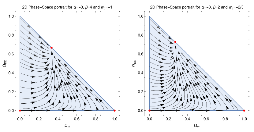
Figure 4: Lotka-Volterra: Phase-space portraits for the dynamical system (52), (53) for $w_{d}=\frac{1-\beta}{3}$,$~{}\alpha=-3$ with $\beta=4$ (left fig.) and $\beta=3$ (right fig.). The physical accepted stationary points are marked with red dots. The unique attactor in the two figures is point $\bar{A}_{2}$ which describes a universe with a coexistence of dark matter and dark energy.

Figure 5: Lotka-Volterra: Qualitative evolution of the energy density parameters $\Omega_{m},~{}\Omega_{DE}$ and $\Omega_{r}$ for the dynamical system (52), (53) for values of the free parameters such that the future attractor is point $\bar{A}_{2}$

Figure 6: Lotka-Volterra: Qualitative evolution of $w_{eff}$ for values of the free parameters such that the future attractor of the dynamical system (52), (53) is point $\bar{A}_{2}$ and initial conditions are that of Fig. 5.

V Dark Energy - Dark Matter - Dark Radiation

Dark radiation is an exotic form of radiation which has been proposed to interact only with dark matter dr1 ; dr2 .

We introduce the energy momentum tensor

$$T_{\mu\nu}^{R}=\left(\rho_{R}+p_{R}\right)u_{\mu}u_{\nu}+p_{R}g_{\mu\nu}~{},~{}p_{R}=\frac{1}{3}\rho_{R},$$ (54)

which we assume describes the dark radiation. The total energy momentum of the universe is defined as

$$T_{\mu\nu}=T_{\mu\nu}^{m}+T_{\mu\nu}^{DE}+T_{\mu\nu}^{R},$$ (55)

and using the Bianchi identity we can now define the following system

$$\left(T_{\mu\nu}^{m}g^{\nu\kappa}\right)_{;\kappa}=Q-V~{},~{}\left(T_{\mu\nu}^{DE}g^{\nu\kappa}\right)_{;\kappa}=-Q~{},~{}\left(T_{\mu\nu}^{R}g^{\nu\kappa}\right)_{;\kappa}=V,$$ (56)

where the new variable $V$ describes the interaction between dark matter and dark radiation.

V.1 The EMR Model

We consider the compartmental interaction with the parameter $Q$ defined by expression (20), and we define the parameter $V$ as $V=V_{0}\left(t\right)\rho_{m}$.

Hence, in the spatially flat FLRW background, equations (56) read as

$$\dot{\rho}_{m}+3H\rho_{m} = Q_{0}\left(t\right)\rho_{m}\rho_{d}-V_{0}\left(t\right)\rho_{m}.$$ (57)

$$\dot{\rho}_{d}+3\left(1+w_{d}\right)H\rho_{d} = -Q_{0}\left(t\right)\rho_{m}\rho_{d},$$ (58)

$$\dot{\rho}_{R}+\frac{4}{3}H\rho_{R} = V_{0}\left(t\right)\rho_{m}.$$ (59)

This dynamical system defines an analogue of a SIR model for cosmology. We shall call it the dark EMR model. In an SIR model, the interaction is between an infected population and a recovered population. In this analogue, the interaction is between dark matter and dark radiation.

We proceed with the analysis of the asymptotics.

V.1.1 Asymptotic analysis

We introduce a new dimensionless variable $\Omega_{R}=\frac{\rho_{R}}{3H^{2}}$, and we write the cosmological field equations in an equivalent form

$$\frac{d\Omega_{m}}{d\tau} = \left(3\left(\alpha+w_{d}\right)\Omega_{DE}+\Omega_{R}-\gamma\right)\Omega_{m},$$ (60)

$$\frac{d\Omega_{DE}}{d\tau} = 3\Omega_{DE}\left(w_{d}\left(\Omega_{DE}-1\right)-\alpha\Omega_{m}\right)+\Omega_{DE}\Omega_{R},$$ (61)

with constraint

$$\Omega_{R}=1-\Omega_{m}-\Omega_{DE}.$$ (62)

Finally the equation of state parameter for the total cosmological fluid is defined as

$$w_{eff}=w_{d}\Omega_{DE}+\frac{1}{3}\Omega_{R}.$$ (63)

We proceed with an analysis of the asymptotic behaviour.

Stationary points

The stationary points $B=\left(\Omega_{m}\left(B\right),\Omega_{DE}\left(B\right)\right)$ of the two-dimensional system (60), (61) are $B_{1}=\left(1-\gamma,0\right),~{}B_{2}=\left(1,0\right)$, $B_{3}=\left(0,0\right)$ and $B_{4}=\left(\frac{\left(1-3w_{d}\right)}{3\alpha}\left(1-\frac{\gamma}{3\left(\alpha+w_{d}\right)}\right),-\frac{1}{3\alpha}+\frac{\gamma\left(1+3\alpha\right)}{9\alpha\left(\alpha+w_{d}\right)}\right)$.

The asymptotic solution at point $B_{1}$ describes a universe with dark matter and dark radiation, i.e. $\Omega_{R}\left(B_{1}\right)=\gamma$. The point is physically accepted for $0<\gamma<1$. This means that there is energy transfer from dark matter to the dark radiation fluid. Points $B_{2}$ and $B_{3}$ have the same physical properties with that of points $A_{2}$ and $A_{3}$, respectively. Indeed, the point $B_{2}$ describes a universe where only dark energy contributes to the cosmological fluid, while at the point $B_{3}$ the asymptotic solution describes a universe dominated by the radiation fluid.

Finally, point $B_{4}$ is an extension of the previous point $A_{4}$, where the three fluids contribute in the universe $\Omega_{R}\left(B_{4}\right)=1-\frac{\gamma-3w_{d}}{3\alpha}$ and $w_{eff}\left(B_{4}\right)=\frac{1}{3}\left(1-\frac{\left(1-3w_{d}\right)}{3\left(\alpha+w_{d}\right)}\gamma\right)$. If we require that point $B_{1}$, which describes the matter era, exist always, that is, $0<\gamma<1$, then point $B_{4}$ is physical accepted when $\left\{0<\alpha<\frac{1}{3},-\alpha<w_{d}<0,\frac{3\left(\alpha+w_{d}\right)}{1+3\alpha}\leq\gamma\leq 3\left(\alpha+w_{d}\right)\right\}$,   or $\alpha>\frac{1}{3}$ and$~{}\left\{-\alpha<w_{d}<\frac{\left(1-3\alpha\right)}{3},\frac{3\left(\alpha+w_{d}\right)}{1+3\alpha}\leq\gamma\leq 3\left(\alpha+w_{d}\right)\right\}$ or $\left\{\frac{\left(1-3\alpha\right)}{3}<w_{d}<0,\frac{3\left(\alpha+w_{d}\right)}{1+3\alpha}\leq\gamma\leq 1\right\}$ For $w_{d}=-1$, the latter conditions becomes $\left\{1<\alpha<\frac{4}{3}~{},~{}\frac{3\left(\alpha-1\right)}{1+3\alpha}\leq\gamma\leq 3\left(\alpha-1\right)\right\},$ or $\left\{\alpha>\frac{4}{3},\ ~{}\frac{3\left(\alpha-1\right)}{1+3\alpha}\leq\gamma\leq 1\right\}$.

As far as the stability properties of the stationary points are concerned, point $B_{1}$ is an attractor for $\alpha>\frac{3w_{d}-\gamma}{3\left(\gamma-1\right)}$ while $B_{2}$ is an attractor for $\alpha<\frac{1}{3}\left(\gamma-3w_{d}\right)$. Furthermore, the point $B_{3}$ always describes an unstable solution. The eigenvalues of the linearized system (60), (61) around the stationary point $B_{4}$ are $e_{1}\left(B_{4}\right)=\frac{\left(3w_{d}-1\right)\alpha\gamma+\sqrt{\bar{D}\left(\alpha,w_{d},\gamma\right)}}{6\alpha\left(\alpha+w_{d}\right)}$, $e_{2}\left(B_{4}\right)=\frac{\left(3w_{d}-1\right)\alpha\gamma-\sqrt{\bar{D}\left(\alpha,w_{d},\gamma\right)}}{6\alpha\left(\alpha+w_{d}\right)}$ in which

$$\bar{D}\left(a,w_{b},\gamma\right)=\left(3w_{d}-1\right)\alpha\left(12\left(\alpha+w_{d}\right)^{2}\left(\left(2+3\alpha\right)\gamma-3\left(\alpha+w_{d}\right)\right)-\alpha\left(5+12\alpha\right)\gamma^{2}\right).$$ (64)

When $\bar{D}\left(\alpha,w_{d},\gamma\right)<0$, then $\frac{\left(3w_{d}-1\right)\alpha\gamma}{6\alpha\left(\alpha+w_{d}\right)}$ and the stationary point can be a stable sink, otherwise for $\bar{D}\left(\alpha,w_{d},\gamma\right)>0$ there are values of the free parameters where the point can be an attractor. Last but not least, for the value of the free variables where point $B_{4}$ is physical accepted, the unique attractor is point $B_{4}$.

In Fig. 7 we present the region space of the free parameters $\left(a,w_{b},\gamma\right)$, where the asymptotic solution described by point $B_{4}$ is stable. The phase-space portrait of the dynamical system (60), (61) are given in 8. Moreover, the qualitative evolution of the physical parameters $\left\{\Omega_{m},\Omega_{DE},\Omega_{R}\right\}$ and $w_{eff}$ are presented in 9 and 10 respectively.

Figure 7: EMR-I: Region space where the asymptotic solution described by point $B_{4}$ is stable.

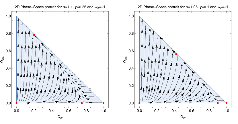
Figure 8: EMR-I: Phase-space portraits for the dynamical system (60), (61) for values of the free parameters where $B_{4}$ is physically accepted. The dynamical space admits four stationary points with $B_{4}$ the unique attractor, and $B_{1}$ a saddle point.

Figure 9: EMR-I: Qualitative evolution of the energy density parameters $\Omega_{m},~{}\Omega_{DE}$ and $\Omega_{r}$ for the dynamical system (60), (61) for values of the free parameters such that $B_{4}$ is physically accepted.

Figure 10: EMR-I: Qualitative evolution of $w_{eff}$ for values of the free parameters such that the future attractor of the dynamical system (60), (61) is the point $B_{4}$ and initial conditions are that of Fig. 9.

VI Quintessence as Dark Energy

In the previous sections, we have assumed that the dark energy has a constant equation of state parameter. However, this assumption suffers from various problems. The simplest gravitational model which describes the dynamical behaviour of the dark energy fluid is the scalar field.

Quintessence is a scalar field minimally coupled to gravity, where in the case of homogeneous spacetimes the corresponding fluid is described by a perfect fluid with energy density $\rho_{\phi}$ and pressure component $p_{\phi}$ defined as

$$\rho_{\phi} = \frac{1}{2}\dot{\phi}^{2}+V\left(\phi\right)~{},$$ (65)

$$p_{\phi} = \frac{1}{2}\dot{\phi}^{2}-V\left(\phi\right)~{},$$ (66)

where $\phi=\phi\left(t\right)$ is the scalar field and $V\left(\phi\right)$ is the potential function which defines the scalar field mass.

The equation of state parameter for the scalar field is calculated as

$$w_{\phi}=\frac{\frac{1}{2}\dot{\phi}^{2}-V\left(\phi\right)}{\frac{1}{2}\dot{\phi}^{2}+V\left(\phi\right)},$$ (67)

from where we observe that $\left|w_{\phi}\right|\leq 1$, and $w_{\phi}\rightarrow-1$, when the scalar field potential$~{}V\left(\phi\right)$ dominates.

When there is no interaction between the scalar field and the dark matter, equation (19) provides the equation of motion for the scalar field, which is a second-order differential equation, that is,

$$\dot{\phi}\left(\ddot{\phi}+3H\dot{\phi}+V_{,\phi}\right)=0.$$ (68)

In the following sections, we investigate the asymptotic dynamics for the two models under consideration, that is, the compartmental interaction model (20) and the Lotka-Volterra interaction model (34). For simplicity of our calculations, we omit the radiation term.

VI.1 The Compartmental Interaction

Consider the interaction in (20) with $Q_{0}\left(t\right)=\alpha\frac{\dot{\phi}}{\sqrt{6}H^{2}}$; which results in the following system

$$\dot{\rho}_{m}+3H\rho_{m} = \alpha\frac{\dot{\phi}}{\sqrt{6}}\frac{\rho_{m}}{H^{2}}\left(\frac{1}{2}\dot{\phi}^{2}+V\left(\phi\right)\right),$$ (69)

$$\ddot{\phi}+3H\dot{\phi}+V_{,\phi} = -\alpha\frac{\rho_{m}}{\sqrt{6}H^{2}}\left(\frac{1}{2}\dot{\phi}^{2}+V\left(\phi\right)\right).$$ (70)

VI.1.1 Asymptotic analysis

We employ the $H$-normalization approach, thus, in terms of new dimensionless variables

$$x=\frac{\dot{\phi}}{\sqrt{6}H}~{},~{}y=\frac{\sqrt{V\left(\phi\right)}}{\sqrt{3}H}~{},~{}\Omega_{m}=\frac{\rho_{m}}{3H^{2}}~{},~{}\lambda=\frac{V_{,\phi}}{V}~{},~{}\tau=\ln a$$ (71)

the field equations read as

$$\frac{dx}{d\tau} = \frac{1}{2}\left[3x\left(x^{2}-y^{2}-1\right)-\sqrt{6}\lambda y^{2}-3\alpha\left(x^{2}+y^{2}\right)\Omega_{m}\right],$$ (72)

$$\frac{dy}{d\tau} = \frac{1}{2}y\left[3+\sqrt{6}\lambda x+3\left(x^{2}-y^{2}\right)\right],$$ (73)

$$\frac{d\lambda}{d\tau} = \sqrt{6}x\lambda^{2}\left(\Gamma\left(\lambda\right)-1\right)~{},~{}\Gamma\left(\lambda\right)=\frac{V_{,\phi\phi}V}{V_{,\phi}^{2}},$$ (74)

with the constraint equation

$$\Omega_{m}=1-x^{2}-y^{2}.$$ (75)

From the constraint equation it follows that $1-x^{2}-y^{2}\geq 0$, which means that $x,y$ take values in the two unitary disk. Furthermore, by definition, $y>0$. Recall that the energy density for the scalar field $\Omega_{\phi}$ is defined as $\Omega_{\phi}=x^{2}+y^{2}$.

Last, but not least, in terms of the new variables the effective equation of state parameter is defined as

$$w_{eff}\left(x,y,\lambda\right)=x^{2}-y^{2}.$$ (76)

For simplicity of our calculations and in order to keep the number of dimensions and the free parameters of the dynamical system low, we assume that the scalar field potential has a constant potential function $V\left(\phi\right)=V_{0}$. This means that the mass of the scalar field as given by equation (70) depends on the energy density of dark matter.

Furthermore, the parameter $\lambda$ is always zero. Thus the dynamical evolution of the physical variables for this model is given by the two-dimensional dynamical system

$$\frac{dx}{d\tau} = \frac{1}{2}\left[3x\left(x^{2}-y^{2}-1\right)-3\alpha\left(x^{2}+y^{2}\right)\left(1-x^{2}-y^{2}\right)\right]\;,$$ (77)

$$\frac{dy}{d\tau} = \frac{1}{2}y\left[3+3\left(x^{2}-y^{2}\right)\right]\;.$$ (78)

Stationary points

The stationary points of the dynamical system (77), (78) are defined on the two-dimensional plane $T=\left(x\left(T\right),y\left(T\right)\right)$, with coordinates $T_{1}=\left(0,0\right)$,  $T_{2}^{\pm}=\left(\pm 1,0\right)$, $T_{3}=\left(-\frac{1}{\alpha},0\right)$, $T_{4}=\left(0,1\right)$ and $T_{5}=\left(x_{4}\left(\alpha\right),\sqrt{1+x_{4}^{2}\left(\alpha\right)}\right)$.

The point $T_{1}$ with $\Omega_{m}\left(T_{1}\right)=1$ describes the matter-dominated era. The linearized system around the stationary points provides the eigenvalues $e_{1}\left(T_{1}\right)=-\frac{3}{2}$ and $e_{2}\left(T_{1}\right)=\frac{3}{2}$, from which we infer that the matter solutions are always unstable and $T_{1}$ is a saddle point.

On the other hand, $T_{2}^{\pm}$ describe solutions where the universe is dominated by the kinetic term of the scalar field, $\Omega_{m}\left(T_{2}^{\pm}\right)=0$, and the effective cosmological fluid is that of stiff matter, i.e. $w_{eff}\left(T_{2}^{\pm}\right)=1$. The corresponding eigenvalues are $e_{1}\left(T_{2}^{\pm}\right)=3$ and $e_{2}\left(T_{2}^{\pm}\right)=3\left(1\pm\alpha\right)$. Thus, asymptotic solutions are always unstable. $T_{2}^{+}$ is a saddle point for $\alpha<-1$, otherwise it is a source, while $T_{2}^{-}$ is a saddle point for $\alpha>1$, otherwise it is also a source.

The point $T_{3}$ describes an asymptotic solution where the kinetic term of the scalar field and the dark matter contribute to the cosmological fluid, i.e. $\Omega_{m}\left(T_{3}\right)=1-\frac{1}{\alpha^{2}}$. The point is physically accepted for $\alpha^{2}>1$, while when $\alpha^{2}=1$ it reduces to the points $T_{2}^{\pm}$. For the cosmological fluid we calculate $w_{eff}\left(T_{3}\right)=\frac{1}{\alpha^{2}}$, which means that it can not describe acceleration. Nevertheless, for $\alpha=\frac{1}{\sqrt{3}}$, point $T_{3}$ describes the radiation solution. The eigenvalues are $e_{1}\left(T_{3}\right)=\frac{3\left(1+\alpha^{2}\right)}{2\alpha^{2}}$, $e_{2}\left(T_{3}\right)=-\frac{3\left(1-\alpha^{2}\right)}{2\alpha^{2}}$, from where we infer that the point when it is physically accepted is a saddle point, otherwise it is a source.

The stationary point $T_{4}$ is an attractor, $e_{1}\left(T_{4}\right)=-3$, $e_{2}\left(T_{4}\right)=-3$, and the asymptotic solution is that of the de Sitter universe, $w_{eff}\left(T_{4}\right)=-1$, $\Omega_{m}\left(T_{4}\right)=0$.

Finally, for point $T_{5},$ parameter $x_{4}$ is given by the equation $\alpha=\frac{1}{x_{4}\left(1+2x_{4}^{2}\right)}$. However, $y\left(T_{5}\right)=\sqrt{1+x_{4}^{2}\left(\alpha\right)}>1$, that is, the point is not physically accepted. The eigenvalues of the linearized system are $e_{1}\left(T_{5}\right)=\frac{3\left\{-1+\sqrt{5+4x_{4}^{2}\left[9+4x_{4}^{2}\left(5+3x_{4}^{2}\right)\right]}\right\}}{2\left(1+2x_{4}^{2}\right)}$, $e_{1}\left(T_{5}\right)=\frac{3\left\{-1-\sqrt{5+4x_{4}^{2}\left[9+4x_{4}^{2}\left(5+3x_{4}^{2}\right)\right]}\right\}}{2\left(1+2x_{4}^{2}\right)}$, thus $T_{5}$ is always a saddle point.

In Fig. 11 we present phase-space diagrams for the dynamical system (77), (78), where we observe that $T_{4}$ is the unique attractor. Moreover, in Figs. 12 and 13 we present the qualitative evolution of the physical parameters $\Omega_{m},~{}\Omega_{\phi}$ and $w_{eff}$ for various sets of initial conditions.

At this point, it is important to mention that for $\alpha^{2}\leq 1$, the physically accepted stationary points are only those of the quintessence model without interaction. Therefore, the physically accepted stationary points that describe non-zero interaction exist only when $\alpha^{2}>1$.

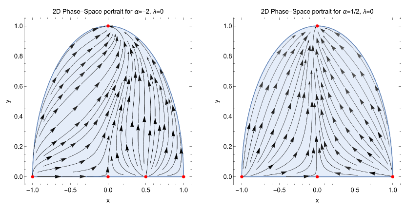
Figure 11: Quintessence (Compartmental): Phase-space portraits for the dynamical system (77), (78) for $\alpha=-2$ (left fig.) and $\alpha=\frac{1}{2}$ (right fig.) The stationary points are marked with red dots. We remark that the unique attractor is point $T_{4}$. However, the structure of the phase-space is different when point $T_{3}$ exist.

Figure 12: Quintessence (Compartmental): Qualitative evolution of the energy density parameters $\Omega_{m}$ and$~{}\Omega_{\phi}$ the dynamical system (77), (78) for $\alpha=-2$, and different sets of initial conditions.

Figure 13: Quintessence (Compartmental): Qualitative evolution $w_{eff}$ as it is given by the solution of the dynamical system (77), (78) and initial conditions of that of Fig. 12. The de Sitter universe described by point $T_{4}$ is the unique future attractor.

VI.2 The Lotka-Volterra Interaction

For the Lotka-Volterra interaction (34) with $Q_{0}\left(t\right)=\alpha\frac{\dot{\phi}}{\sqrt{6}H^{2}}$ and $Q_{1}\left(t\right)=\beta\frac{\dot{\phi}^{2}}{H}$, in terms of the dimensionless variables the field equations are expressed as follows

$$\frac{dx}{d\tau} = \frac{1}{2}\left[3x\left(x^{2}-y^{2}-1\right)-\sqrt{6}\lambda y^{2}-3\left(x^{2}+y^{2}\right)\left(\alpha\Omega_{m}+2\beta x\right)\right],$$ (79)

$$\frac{dy}{d\tau} = \frac{1}{2}y\left[3+\sqrt{6}\lambda x+3\left(x^{2}-y^{2}\right)\right],$$ (80)

$$\frac{d\lambda}{d\tau} = \sqrt{6}x\lambda^{2}\left(\Gamma\left(\lambda\right)-1\right)~{},~{}\Gamma\left(\lambda\right)=\frac{V_{,\phi\phi}V}{V_{,\phi}^{2}}.$$ (81)

with algebraic constraint (75).

Hence, by applying the constraint (75) and we consider a constant potential function, that is, $\lambda=0$, we end with the two-dimensional system

$$\frac{dx}{d\tau} = \frac{1}{2}\left[3x\left(x^{2}-y^{2}-1\right)-\sqrt{6}\lambda y^{2}-3\left(x^{2}+y^{2}\right)\left(\alpha\left(1-x^{2}-y^{2}\right)+2\beta x\right)\right],$$ (82)

$$\frac{dy}{d\tau} = \frac{1}{2}y\left[3+\sqrt{6}\lambda x+3\left(x^{2}-y^{2}\right)\right].$$ (83)

Stationary points

The stationary points $\bar{T}=\left(x\left(\bar{T}\right),y\left(\bar{T}\right)\right)$ of the two dimensional dynamical system (82), (83), have the following coordinates, $\bar{T}_{1}=\left(0,0\right)$, $\bar{T}_{2}=\left(0,1\right)$, $\bar{T}_{3}=\left(x_{3}\left(\alpha,\beta\right),0\right)$ and $\bar{T}_{4}=\left(x_{4}\left(\alpha,\beta\right),\sqrt{1+\left(x_{4}\left(\alpha,\beta\right)\right)^{2}}\right)$. We proceed with a discussion of the physical properties for the asymptotic solutions at the stationary points.

The asymptotic solution at point $\bar{T}_{1}$ describes a universe dominated by the matter era, similar to point $T_{1}$. The eigenvalues are calculated $e_{1}\left(\bar{T}_{1}\right)=-\frac{3}{2}$, $e_{2}\left(\bar{T}_{2}\right)=\frac{3}{2}$, which means that $\bar{T}_{1}$ is always a saddle point.

Moreover, point $\bar{T}_{2}$ describes the de Sitter solution as point $T_{4}$. The eigenvalues are $e_{1}\left(\bar{T}_{2}\right)=-3$, $e_{2}\left(\bar{T}_{2}\right)=-3\left(1+\beta\right)$. Hence, $\bar{T}_{2}$ is an attractor when $\beta>-1$.

For the stationary point $\bar{T}_{3}$, parameter $x_{3}\left(\alpha,\beta\right)$ is given by the algebraic equation $\beta=\frac{\left(1+\alpha x_{3}\right)\left(x_{3}^{2}-1\right)}{2x_{2}}$, where for $\beta=0$, the points $T_{2}^{\pm}$ and $T_{3}$ are recovered. The asymptotic solution at the point $\bar{T}_{3}$, cannot describe acceleration, i.e., $w_{eff}\left(\bar{T}_{3}\right)=\left(x_{3}\right)^{2}\geq 0$. We remark that $\bar{T}_{3}$ can describe one or three real points. We calculate the eigenvalues $e_{1}\left(\bar{T}_{3}\right)=\frac{3}{2}\left(1+x_{3}^{2}\right)$ and $e_{2}\left(\bar{T}_{3}\right)=\frac{3}{2}\left(2+\alpha x_{3}\left(1+x_{3}^{2}\right)\right)$. Hence, point $\bar{T}_{3}$ always describes an unstable solution.

Finally, the point $\bar{T}_{4}$ is not physically accepted because $y\left(\bar{T}_{4}\right)>0$. Function $x_{4}\left(\alpha,\beta\right)$ is given by the algebraic equation $\beta=\alpha x_{4}-\frac{1}{1+2x_{4}^{2}}$. The eigenvalues of the linearized system near to the stationary point are $e_{1}\left(\bar{T}_{4}\right)=\frac{3}{2\left(1+2x_{4}^{2}\right)}\left(-1+\sqrt{1+4x_{4}\left(1+x_{4}^{2}\right)\left(1+2x_{4}^{2}\right)\left(\alpha+4x_{4}\left(1+\alpha x_{4}\left(1+x_{4}^{2}\right)\right)\right)}\right)$ and $e_{2}\left(\bar{T}_{4}\right)=\frac{3}{2\left(1+2x_{4}^{2}\right)}\left(-1-\sqrt{1+4x_{4}\left(1+x_{4}^{2}\right)\left(1+2x_{4}^{2}\right)\left(\alpha+4x_{4}\left(1+\alpha x_{4}\left(1+x_{4}^{2}\right)\right)\right)}\right)$. From these eigenvalues it is clear that $\bar{T}_{4}$ can be an attractor. However, this will be unphysical and the free parameters $\alpha$, $\beta$ should be constrained such that $\bar{T}_{4}$ is a source or saddle point.

In Fig. 14 we present the contour plot that relates the free parameters $\alpha\;,\beta$ and $x_{4}$; we also present the region where the real parts of the eigenvalues are negative. We observe that the model is physically accepted approximately for $\beta>-1$. Phase-space portraits of the two-dimensional dynamical system (82), (83) are given in Fig. 15. Finally, the evolution of the physical parameters $\Omega_{m},~{}\Omega_{\phi}$ and $w_{eff}$ are given in Figs. 16 and 17. The values of the free parameters have been selected such that the unique attractor is the de Sitter point $\bar{T}_{2}$.

Figure 14: Quintessence (Lotka-Volterra): Left fig.: Contour plot which relates the values $x_{4},~{}\alpha$ and $\beta$. Right fig.: Region when point $\bar{T}_{4}$ is an attractor.

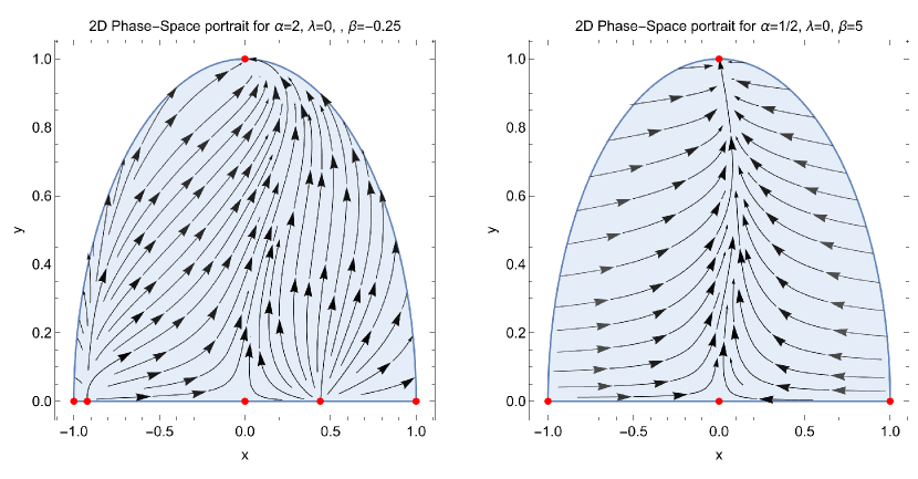
Figure 15: Quintessence (Lotka-Volterra): Phase-space portraits for the dynamical system (82), (83) for $\alpha=-2$, $\beta=-\frac{1}{4}$ (left fig.) and $\beta=5$ (right fig.) The stationary points are marked with red dots. The unique attractor is the de Sitter point $T_{2}$.

Figure 16: Quintessence (Lotka-Volterral): Qualitative evolution of the energy density parameters $\Omega_{m}$ and$~{}\Omega_{\phi}$ the dynamical system (82), (83) for $\alpha=-2$, $\beta=-\frac{1}{4}$ and different sets of initial conditions.

Figure 17: Quintessence (Lotka-Volterra): Qualitative evolution $w_{eff}$ as it is given by the solution of the dynamical system (77), (78) and initial conditions of that of Fig. 16. The de Sitter universe described by point $T_{2}$ is the unique future attractor.

VII Conclusions

Cosmological models with interaction in the dark sector are crucial for describing the universe. Due to the interaction, new degrees of freedom are introduced into the gravitational model, which drive the dynamics and help explain the observations.

In this study, we examined gravitational models that describe compartmentalization and co-existence in the dark sector of the universe. Drawing inspiration from population dynamics models in biology, we analogized dark energy and dark matter as two species evolving in the “universe.” Furthermore, dark radiation was introduced as the third “species.”

To study the interaction models, we employed dynamical analysis and a phase-space investigation. We used the H-normalization approach and calculated the asymptotic solutions and their stability properties in terms of dimensionless variables. Each asymptotic solution corresponds to a specific stationary point of the cosmological field equations, representing a distinct era of cosmic evolution.

We considered dark matter to be described by a pressureless fluid source, while for dark energy we assumed two cases. In the first case, dark energy is described by an ideal gas with a constant equation of state parameter. In the second scenario, we considered dark energy as described by a quintessence scalar field. Due to the potential function, the dynamics of the second cosmic scenario leads to a more complex cosmological history. From this analysis, we can provide constraints on the dynamical variables of the interacting model and discuss the cosmological viability of the models.

In future work, we plan to investigate whether such interacting models can help reduce cosmological tensions.

From this research, the interactions between dark matter and dark energy could significantly influence the dynamics of the universe. The study demonstrates that these interactions could potentially address cosmological tensions such as $H_{0}$ and $\sigma_{8}$ tensions, suggesting that the interaction terms might be key to solving some persistent problems in cosmology.

Furthermore, the models analysed show varied asymptotic behaviours, indicating the complexity and sensitivity of cosmic evolution to the specific characteristics of dark sector interactions. We conclude that understanding these interactions not only provides insights into the nature of dark matter and dark energy but also helps in predicting the future dynamics of the universe.

The analysis and results underscore the importance of considering different interaction models and their implications on cosmological scales. In future work, we plan to investigate the extent to which such interacting models can help reduce cosmological tensions. This research lays a foundational framework for such investigations, highlighting the critical role of theoretical models in cosmology.

Data Availability Statements: Data sharing is not applicable to this article as no datasets were generated or analyzed during the current study.

References

• (1) D. W. Sciama, Modern Cosmology and the Dark Matter Problem, Cambridge University Press, Cambridge (1994)
• (2) L. Amendola and S. Tsujikawa, Dark Energy: Theory and Observations, Cambridge University Press, Cambridge (2013)
• (3) A.G. Riess et al., Observational Evidence from Supernovae for an Accelerating Universe and a Cosmological Constant, Astron. J. 116, 1009 (1998)
• (4) M. Kowalski et al., The Three-Dimensional Power Spectrum of Galaxies from the Sloan Digital Sky Survey, Astrophys. J. 686, 749 (2008)
• (5) L. Perivolaropoulos and F. Skara, Challenges for $\Lambda$CDM: An update, New Astronomy Reviews 95, 101659 (2022)
• (6) A. Nicolis, R. Rattazzi and E. Trincherini, Phys. Rev. D 79, 064036 (2009)
• (7) C. Deffayet, G. Esposito-Farese and A. Vikman, Phys. Rev. D 79, 084003 (2009)
• (8) G.W. Horndeski, Int. J. Ther. Phys. 10, 363 (1974)
• (9) L. Arturo Ureña-López, J. Phys. Conf. Ser. 761, 012076 (2016)
• (10) B. Ratra and P.J.E Peebles, Phys. Rev. D 37, 3406 (1988)
• (11) A. Linde, D-Term Inflation, Phys. Rev. D 49, 748 (1994)
• (12) E.O. Kahya and B. Pourhassa, The universe dominated by the extended Chaplygin gas, Astroph. Space Sci. 353, 677 (2014)
• (13) O. Bertolami and V. Duvvuri, Chaplygin inspired Inflation, Phys. Lett. B 640, 121 (2006)
• (14) C. Brans and R.H. Dicke, Phys. Rev. 124, 195 (1961)
• (15) J. O’Hanlon, Phys. Rev. Lett. 29 137 (1972)
• (16) K.-i. Maeda and N. Ohta, Phys. Lett. B 597, 400 (2004)
• (17) R. Ferraro and F. Fiorini, Phys. Rev. D 75, 084031 (2007)
• (18) R. Ferraro and F. Fiorini, Phys. Rev. D 78, 124019 (2008)
• (19) A. Paliathanasis, J.D. Barrow and P.G.L. Leach, Cosmological solutions of f(T) gravity, Phys. Rev. D 94, 023525 (2016)
• (20) S. Nojiri and S.D. Odintsov, Phys. Lett. B 631, 1 (2005)
• (21) T. Clifton, Spherically symmetric solutions to fourth-order theories of gravity, Class. Quant. Grav. 23, 7445 (2006)
• (22) L. Heisenberg, Review on f(Q) gravity, Physics Reports 1066, 1 (2024)
• (23) L. Amendola, Phys. Rev. D 62, 043511 (2000)
• (24) R.-G. Cai and A. Wang, Cosmology with interaction between phantom dark energy and dark matter and the coincidence problem, JCAP 03, 002 (2005)
• (25) L. Amendola, G.C. Campos and R. Rosenfeld, Consequences of dark matter-dark energy interaction on cosmological parameters derived from type Ia supernova data, Phys. Rev. D 75, 083506 (2007)
• (26) J. F. Jesus, A. A. Escobal, D. Benndorf and S. H. Pereira, Can dark matter–dark energy interaction alleviate the cosmic coincidence problem?, Eur. Phys. J. C 82, 273 (2022)
• (27) N. Cruz, S. Lepe and F. Pena, Dark energy interacting with two fluids, Phys. Lett. B 663, 338 (2008)
• (28) J.M. Salim and S.L. Sautú, Gravitational theory in Weyl Integrable Spacetime, Class. Quantum Grav. 13, 353 (1996)
• (29) J.M. Salim and S.L. Sautu, Gravitational collapse in Weyl Integrable Spacetimes, Class. Quantum Grav. 16, 3281 (1999)
• (30) J. Khoury and A. Wetlman,Phys. Rev. Lett. 93, 171104 (2004)
• (31) L. Amendola, Coupled Quintessence, Phys. Rev. D 62, 043511 (2000)
• (32) V. Faraoni, Cosmology in Scalar-Tensor Gravity, Kluwer Academic Publishers, Dordrecht, (2004)
• (33) G. Leon and A. Paliathanasis, Stability of a modified Jordan-Brans-Dicke theory in the dilatonic frame, Gen. Rel. Grav. 52, 71 (2020)
• (34) Y.-F. Cai, E.N. Saridakis, M.R. Setare and J.-Q. Xia, Phys. Rept. 493, 1 (2010)
• (35) A. Paliathanasis, Class. Quantum Grav. 37, 195014 (2020)
• (36) S.V. Chervon, Quantum Matter 2, 71 (2013)
• (37) A. R. Brown, Phys. Rev. Lett. 121, 251601 (2018)
• (38) S. Kumar and R. C. Nunes, Phys. Rev. D 96, no. 10, 103511 (2017)
• (39) E. Di Valentino, A. Melchiorri and O. Mena, Phys. Rev. D 96, 043503 (2017)
• (40) S. Pan, W. Yang and A. Paliathanasis, MNRAS 493, 3114 (2020)
• (41) S. Kumar, R. C. Nunes and S. K. Yadav, Eur. Phys. J. C 79, no. 7, 576 (2019)
• (42) A. Pourtsidou and T. Tram, Phys. Rev. D 94, no. 4, 043518 (2016)
• (43) R. An, C. Feng and B. Wang, JCAP 1802, no. 02, 038 (2018)
• (44) M. Lucca, Dark energy–dark matter interactions as a solution to the S8 tension, Phys. Dark Univ. 34, 100899 (2021)
• (45) V. Poulin, J.L. Bernal, E. Kovetz and M. Kamionkowski, The Sigma-8 Tension is a Drag, Phys. Rev. D 107, 123538 (2023)
• (46) J. Gleyzes, D. Langlois, M. Mancarella and F. Vernizzi, JCAP 1508, 054 (2015)
• (47) C. G. Böehmer, N. Tamanini and M. Wright, Phys. Rev. D 91, no. 12, 123002 (2015)
• (48) C. G. Böehmer, N. Tamanini and M. Wright, Phys. Rev. D 91, no. 12, 123003 (2015)
• (49) S. Pan, G. S. Sharov and W. Yang, Phys. Rev. D 101, no.10, 103533 (2020)
• (50) G. D’Amico, T. Hamill and Nemanja Kaloper, Phys. Rev. D 94, 103526 (2016)
• (51) S. Pan, J. de Haro, W. Yang and J. Amorós, Phys. Rev. D 101, no.12, 123506 (2020)
• (52) D. Pavón and B. Wang, Gen. Rel. Grav. 41, 1 (2009)
• (53) L. P. Chimento, Phys. Rev. D 81, 043525 (2010)
• (54) W. Yang, S. Pan and J. D. Barrow, Phys. Rev. D 97, no. 4, 043529 (2018)
• (55) M. Thorsrud, D. F. Mota and S. Hervik, JHEP 1210, 066 (2012)
• (56) S. Pan, S. Bhattacharya and S. Chakraborty, Mon. Not. Roy. Astron. Soc. 452, 3038 (2015)
• (57) S. Pan and G. S. Sharov, Mon. Not. Roy. Astron. Soc. 472, 4736 (2017)
• (58) G. Caldera-Cabral, R. Maartens, L.A. Ureña-López, Phys. Rev. D 79, 063518 (2009)
• (59) A. Paliathanasis, S. Pan and W. Yang, Int. J. Mod. Phys. D 28, 1950161 (2019)
• (60) M.A. van der Westhuizen and A. Abebe, Interacting dark energy: clarifying the cosmological implications and viability conditions, JCAP 01, 048 (2024)
• (61)
• (62) E. González, C. Maldonado, N. S. Mite and R. Salinas, WIMP dark matter in bulk viscous non-standard cosmologies (2024) [arXiv:2409.03083 [hep-ph]].
• (63) Y.C. Ong, Universe 9, 437 (2023)
• (64) L. Amendola, D. Polarski and S. Tsujikawa, IJMPD 16, 1555 (2007)
• (65) G. Leon and E.N. Saridakis, JCAP 1504, 031 (2015)
• (66) G. Leon and E.N. Saridakis, JCAP 1504, 031 (2015)
• (67) T. Gonzales, G. Leon and I. Quiros, Class. Quantum Grav. 23, 3165 (2006)
• (68) A. Giacomini, S. Jamal, G. Leon, A. Paliathanasis and J. Saveedra, Phys. Rev. D 95, 124060 (2017)
• (69) G. Acquaviva and Nihan Katirci, Dynamical analysis of logarithmic energy–momentum squared gravity, Phys. Dark Univ. 38, 101128 (2024)
• (70) S. Mishra and S. Chakraborty, EPJC 79, 328 (2019)
• (71) L. Chen, Dynamical analysis of loop quantum $R^{2}$ cosmology, Phys. Rev. D 99, 06425 (2018)
• (72) A. Chattrerjee, Dynamical analysis of coupled curvature-matter scenario in viable f(R) dark energy models at de Sitter phase, Class. Quantum Grav. 41, 095007 (2024)
• (73) G. Acquaviva and A. Beesham, Dynamical analysis of a first order theory of bulk viscosity, Class. Quantum Grav. 35, 195011 (2018)
• (74) A. Algo, C. Uggla and J. Wainwright, Perturbations of the Lambda-CDM model in a dynamical systems perspective, JCAP 09, 045 (2019)
• (75) S. Basilakos, G. Leon, G. Papagiannopoulos and E.N. Saridakis, Dynamical system analysis at background and perturbation levels: Quintessence in severe disadvantage comparing to $\Lambda$CDM, Phys. Rev. D 100, 043524 (2014)
• (76) S. Pan, W. Yang, E. Di Valentino, D. F. Mota and J. Silk, IWDM: the fate of an interacting non-cold dark matter — vacuum scenario, JCAP 07 (2023), 064
• (77) D. Benisty, S. Pan, D. Staicova, E. Di Valentino and R. C. Nunes, Late-Time constraints on Interacting Dark Energy: Analysis independent of $H_{0}$, $r_{d}$ and $M_{B}$, Astron. Astrophys. 688 (2024), A156
• (78) G. Mangano, G. Miele and V. Pettorino, Coupled quintessence and the coincidence problem Mod. Phys. Lett. A 18, 831 (2003)
• (79) N.A. Koshelev, On the growth of perturbations in interacting dark energy and dark matter fluids, Gen. Rel. Grav. 43, 1309 (2011)
• (80) Y.C. Ong, An Effective Sign Switching Dark Energy: Lotka–Volterra Model of Two Interacting Fluids, Universe 9, 437 (2023)
• (81) I. Masina, Dark matter and dark radiation from evaporating primordial black holes, Eur. J. Phys. Plus 135, 552 (2020)
• (82) K.V. Berghaus, P.W. Graham, D.E. Kaplan, G.D. Moore, S. Rajendran, Phys. Rev. D 104, 083520 (201)