Enhancing Empathic Accuracy: Penalized Functional Alignment Method to Correct Misalignment in Emotional Perception
Abstract
Empathic accuracy (EA) is the ability to accurately understand another person’s thoughts and feelings, which is crucial for social and psychological interactions. Traditionally, EA is measured by comparing perceivers’ real-time ratings of a target’s emotional states with the target’s self-evaluation. However, these analyses often ignore or simplify misalignments between ratings (such as assuming a fixed delay), leading to biased EA measures. We introduce a novel alignment method that accommodates diverse misalignment patterns, using the square-root velocity representation to decompose ratings into amplitude and phase components. Additionally, we incorporate a regularization term to prevent excessive alignment by constraining temporal shifts within plausible human perception bounds. The overall alignment method is implemented effectively through a constrained dynamic programming algorithm. We demonstrate the superior performance of our method through simulations and real-world applications to video and music datasets.
Keywords: Functional Data Analysis; Warping Function; Regularization; Square Root Velocity Function; Cognitive Study
1 Introduction
Empathic accuracy (EA) measures a person’s ability to correctly identify the internal states of social targets, i.e., the ability to “read people.” Evolutionary theories suggest that empathy has played an important role in human society to help increase cooperation and social cohesion (De Waal,, 2008). On a personal level, EA is critical to social interactions. Impairments in empathy, such as those seen in autism and psychopathy, result in severe deficits in social function (Blair,, 2005). Given its importance related to people’s life quality, empathy has become the focus of a growing amount of research in different fields. For example, in social science, EA’s role was examined in developing and maintaining healthy social relationships (Sened et al.,, 2017). In clinical research, EA has been used as an index to differentiate individuals with certain psychiatric disorders from health controls (Lee et al.,, 2011). Note that the validity of these studies depends on the quality of the inference on EA.
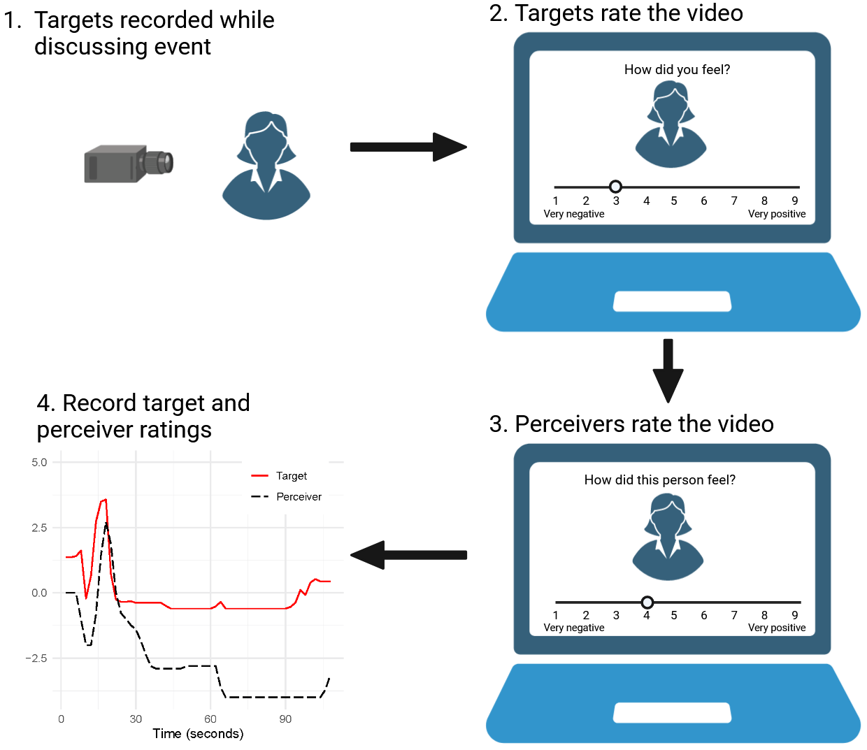
There are two types of studies commonly used to examine EA. One is the non-real-time EA study design, where perceivers provide their response to stimuli after the stimuli have been conducted. The outcome of their overall empathy can be categories of emotion (e.g., happiness, anger, sadness, etc.) or extent of emotion on a Likert-type scale (Ekman,, 1992; Schweinle et al.,, 2002). The other EA study design is the real-time assessment of perceivers’ empathy on an audio or video stimuli (i.e., the recorded affective states of targets) (Zaki et al.,, 2008; Jospe et al.,, 2020), where perceivers provide continuous feedback on their perceptions of the target’s emotional state while the stimuli are unfolding. Illustrated in Figure 1, social targets varying in trait emotional intensity were videotaped while discussing emotional autobiographical events. Perceivers watch these videos and report the perceived emotions in real-time using, for example, a 9-point Likert scale (e.g., 1 = extremely negative; 9 = extremely positive). Compared with the non-real-time EA studies, the real-time design provides more granular information on the dynamic nature of empathy in everyday interactions and detects subtle changes in emotional responses that might be missed in non-real-time assessments.
In this paper, we focus on analyzing data from real-time EA study design. For such design, correlational analysis (Zaki et al.,, 2009; Mackes et al.,, 2018, among others) is a predominant statistical method for examining EA. This approach typically computes a monotonic transformation of the Pearson correlation between the observed perceivers’ responses with targets’ self-reported emotion ratings, where the latter is considered the gold standard. Linear models have also been introduced to investigate the influence of additional factors or unobserved variables on EA. For example, Tabak et al., (2022) proposed a latent variable model that decomposes EA into three separate dimensions: bias, discrimination, and variability. Bias measures the systematic difference between perceiver’s ratings and target’s ratings; discrimination measures perceiver’ sensitivity in relation to target’s ratings; and variability measures the variance of random error in perceiver’s perceptions.
A fundamental assumption in the above correlational and linear model analyses is the alignment of rating sequences between perceivers and targets; in other words, a percever’s rating at a time point is matched and compared with the target’s rating at exactly the same time point. However, this assumption is violated due to the complex cognitive processes in decoding another person’s emotional state. Scherer, (2003) proposed a multi-stage model of emotion decoding, suggesting that perceivers actively interpret various cues (e.g., facial expressions, gestures, vocalizations) to infer target emotions. This complex, real-time process inevitably introduces time discrepancies between perceivers’ and targets’ ratings, leading to substantial misalignments between their respective rating sequences. Traditional data analysis methods, designed for perfectly aligned data, are ill-equipped to handle the misalignment inherent in continuous time-series emotion data, leading to biased results and inflated variability.
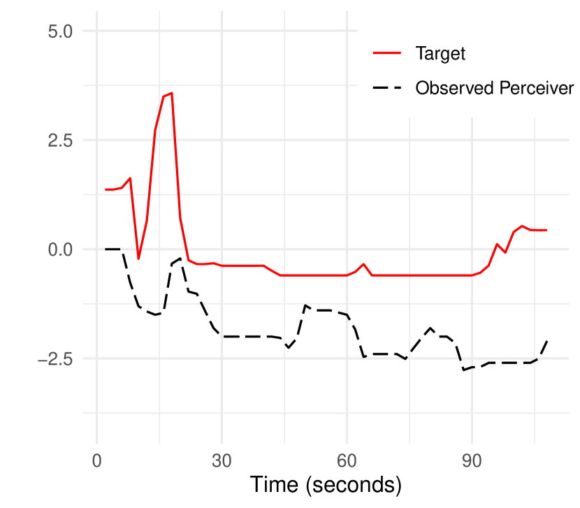
A common approach to address misalignment in EA studies involves introducing a fixed response delay, assuming consistent emotional expression patterns across individuals. This method shifts perceivers’ response time series backward by a predetermined amount (Nicolle et al.,, 2012; Huang et al.,, 2015; Khorram et al.,, 2019). However, Scherer, (2003) countered this assumption, arguing that emotional expressions are diverse and context-dependent. Consequently, the misalignment between perceivers’ and targets’ ratings is more complex than a simple time shift. Figure 2(a) illustrates a typical misalignment between perceiver and target ratings in EA data (Devlin et al.,, 2014). While a delay in perceiver responses is evident, it is not the sole cause of misalignment. For instance, the perceiver’s prolonged sustained response from 10 to 15 seconds, in contrast to the target’s brief dip at 10 seconds, highlights the complex nature of these discrepancies.
To allow a more flexible framework to account for diverse patterns of misalignments than simple time shifts, time series alignment methods aim to preserve data’s geometric structure while enabling accurate statistical analysis. For example, distance time warping (DTW) is a classic approach that aligns time series by minimizing their distance (Sakoe and Chiba,, 1978; Berndt and Clifford,, 1994). However, DTW lacks metric properties and can distort data through the “pinching effect” (Srivastava et al.,, 2011; Marron et al.,, 2015; Zhao et al.,, 2020). While introducing roughness penalties can mitigate the pinching effect (Ramsay and Silverman,, 2005), they may introduce asymmetry (Guo et al.,, 2022). Also, landmark-based methods align time series by matching key points like local maxima and minima (Kneip et al.,, 2000). However, they are sensitive to noise and can lose information due to the discretization of functions using a limited number of landmarks (Wang and Gasser,, 1997; Marron et al.,, 2015). Moreover, these landmark-based methods are not appropriate for our current EA studies, because there is no consensus on how many landmarks are present in these continuous ratings.
Due to the high-frequency nature of the observed EA rating data, we treat each observed curve as a sample path of a continuous function in the time domain, i.e., functional data. Such an approach of representing high-frequency data as functional is common in the literature (Kokoszka and Reimherr,, 2017). From this perspective, misalignment between two observed ratings is caused by a smooth warping function that distorts the time domain of the perceiver in relative to that of the target. Hence, the target and the perceiver’s rating functions can be aligned by estimating this smooth warping function from the observed data, for example, by minimizing an distance between the target and the estimated aligned response function (Ramsay and Li,, 1998). Recently, square root velocity function (SRVF) representations have been employed for aligning two functions (Srivastava et al.,, 2011), and has been increasingly applied across various fields, including biology, medicine, geology, and signal processing (Su et al.,, 2014; Laga et al.,, 2014; Bharath et al.,, 2018; Zhao et al.,, 2020; Mitchell et al.,, 2022). As we will review in Section 2, this SRVF representation leverages the Fisher-Rao metric’s invariance property, so it enables a consistent separation of horizontal component (also known as phase) from vertical component (also known as amplitude), making visualization and summarizing variability in functional datasets more effective (Xie et al.,, 2017).
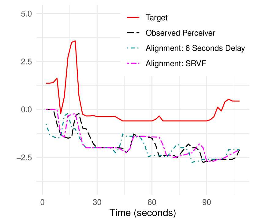
Building upon the SRVF-alignment framework, this paper introduces a novel penalized SRVF-based alignment method for unsynchronized rating sequences in EA studies. Our approach offers both a practical and a methodological innovation. Practically, our proposed method is the first method to study EA that accommodates diverse misalignment patterns (e.g., delays, compressions, and stretches), surpassing the limitations of fixed delay adjustments. Methodologically, our method proposes a penalty term to prevent excessive alignment by constraining temporal shifts within plausible human perception bounds (Levenson,, 1988; Gunes and Pantic,, 2010; Ringeval et al.,, 2015; Mariooryad and Busso,, 2014). Furthermore, the SRVF-based alignment method can be implemented effectively by a constrained dynamic programming algorithm. To highlight the contribution of our method, Figure 2(b) contrasts the proposed penalized SRVF method with a fixed 6-second delay adjustment. Although the 6-second delay adjustment aligns the peaks between the two sequences, it, unfortunately, eliminates the brief 5-second sustain at the start of the perceiver’s sequence, which originally matched up with the target’s self-rating sequence. In contrast, the proposed penalized SRVF-based method has aligned the peaks while keeping the initial sustain in the perceiver’s sequence in place, demonstrating its flexibility in handling complex misalignment patterns. By performing a more accurate alignment step, we will demonstrate that our SRVF-based alignment method provides a more accurate estimation of EA, compared to a serious underestimation when misalignment is ignored and a serious overestimation when no penalty is applied.
The remaining of the paper is structured as follows. Section 2 provides background information on empathic accuracy and existing alignment methods. The proposed methodology is detailed in Section 3. To evaluate the proposed method, Section 4 presents a simulation study and comparisons to alternative approaches. Real-world applications to social and music empathy are explored in Section 5. Finally, Section 6 offers a discussion of the findings and concludes the paper.
2 Background
2.1 Elastic Functional Data Analysis
Functional data often exhibit phase variations, characterized by misaligned geometric features like peaks and valleys (Wu and Srivastava,, 2014; Wallace et al.,, 2014; Tucker et al.,, 2014). A common strategy for addressing these variations involves separating the phase and amplitude components, followed by horizontal alignment of the geometric features through warping techniques.
Let be the target and observed perceiver functions, respectively. We assume that the observed perceiver function has some misalignment. Additionally, we assume that there exists an unobserved, aligned perceiver , which represents the perceiver function without such misalignment. Without loss of generality, functions could be rescaled to and .
In the alignment process, we aim to recover the aligned perceiver function from the observed perceiver function . As the aligned perceiver is unknown, we instead align the perceiver’s response to the target. The alignment problem finds the warping function that transforms the perceiver function that registers its geometric features to the target function by . The transformed perceiver function is expected to align better with the target. A common assumption for this warping function is that it is boundary preserving and smooth (Srivastava and Klassen,, 2016); mathematically, we assume , where
Hence, to align the two functions and , a natural approach is to find a warping function that minimizes the distance between the two functions and , i.e.,
| (1) |
However, the distance between and is not symmetric and the distance-based alignment also suffers from the pinching effect problem where leads to degenerate solutions (Srivastava and Klassen,, 2016). Although there are studies that have addressed the problem by implementing the penalty to (1), the distance-based alignment does not have the appropriate invariance property where .
The Fisher-Rao metric enables a better comparison of functions than the distance. It is an elastic Riemannian metric and has the invariance property, meaning the difference between the functions measured by the Fisher-Rao metric is maintained even after their phases are transformed by the warping function. As a result, using the Fisher-Rao metric in functional alignment can avoid the pinching effect and lead to better functional alignment results. However, the Fisher-Rao metric computation using functions (e.g., and ) is complicated, where only a limited number of algorithms are available (Srivastava et al.,, 2011).
A recently developed method for functional alignment proposes to use the SRVF representation instead of the original representation of and (Srivastava et al.,, 2007, 2011; Srivastava and Klassen,, 2016), which makes it easier to compute the Fisher-Rao metric. In the following, we briefly review the formulation of the SRVF representation. More details can be found in Srivastava and Klassen, (2016).
For any absolute continuous function , the SRVF of is the function , , where . That is, the SRVF of is defined based on its first derivative, representing the continuous changes of over time. If is warped by , the corresponding SRVF of becomes . To ease the notation, we write . Let and be the SRVFs of the target and perceiver functions, respectively, the alignment problem of the target and perceiver using their SRVFs can be solved by finding an optimal warping function
| (2) |
The optimal warping is expected to align two functions so that the transformed function is aligned with . The subscript stands for “unpenalized,” meaning the optimal is not subject to any other constraint than being in the space . This unpenalized alignment has been implemented in the fdasrvf packages (Tucker,, 2023) in both R and Python.
Employing the SRVF representations provides several benefits compared to using the original functions. First, the difference between functions and measured by the Fisher-Rao metric can be easily obtained by the distance between their SRVFs and (Srivastava et al.,, 2007). Second, the pinching effect can be mitigated due to the invariance property of the Fisher-Rao metric, i.e., for any , we have (Srivastava and Klassen,, 2016). As a result, the alignment by maintains the norm of the SRVF . Lastly, using their SRVF representations, functions can be decomposed into phase and amplitude components, which represent distinct sources of variation in functional data (Xie et al.,, 2017). Hence, the differences between functions can be quantified by a proper metric based on the phase and amplitude components. For example, the phase differences between the rescaled functions can be measured by using the warping function obtained by (2). The SRVFs of warping functions lie on the unit Hilbert sphere, allowing us to measure the Fisher-Rao phase distance by the arc length between them on the sphere. It can be approximated by
| (3) |
2.2 Unpenalized SRVF leads to Over-Alignment
While the SRVF representation leads to several theoretical benefits, one primary disadvantage of the unpenalized SRVF for studying EA is that the estimated perceiver function may be overly-aligned with the target and thus could differ from the aligned perceiver function . Particularly, if observed perceiver functions are noisy or include false peaks or valleys due to random variation, they may be incorrectly aligned with real peaks or valleys of targets.
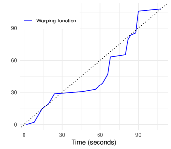
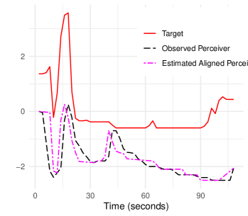
Figure 3(a) shows one example from the study in Devlin et al., (2014) demonstrating the result of the previous SRVF alignment obtained from (2) . In this study, the continuous ratings were recorded for 108 seconds and averaged over 2-second epochs. The alignment is obtained by using their SRVF representations , , and . The estimated warping function is plotted in the right panel of Figure 3(a). When appears above the 45-degree line, it implies that the perceiver’s response is delayed compared to the target, whereas below the 45 degree line indicates that the perceiver’s response precedes the target. For example, the peak of the perceiver’s response around second is considered as a response preceding the target’s self-rating around second, and it is aligned accordingly by the unpenalized SVRF method.
Therefore, from the left plot of Figure 3(a), the unpenalized SRVF method misaligns the peak of the perceiver’s response, occurring at approximately seconds, with the target’s small peak at around seconds, which is likely just a noise. This alignment suggests an improbable scenario where the perceiver predicts the target’s emotional change 25 seconds in advance. Psychological research has consistently shown that perceiver-target unsynchronization is typically limited to a few seconds: 0.5 to 4 seconds (Levenson,, 1988), 3 to 6 seconds (Nicolle et al.,, 2012), 2 to 11 seconds (Mariooryad and Busso,, 2014), and 0.48 to 6.24 seconds (Ringeval et al.,, 2015). By disregarding this inherent limitation, unpenalized SRVF alignment overestimates synchronization between rating sequences, potentially leading to an unrealistic shape of the estimated warping function that exceeds the human exception bounds, and hence biased estimations of perceiver EA levels.
3 Method
3.1 Penalized Elastic Functional Alignment
Penalized alignment has been proposed to control the amount of alignment (Wu and Srivastava,, 2011; Mitchell et al.,, 2022; Guo et al.,, 2022) or to achieve smooth alignment (Srivastava and Klassen,, 2016). To address the over-alignment issue inherent in the unpenalized SRVF method, we employ a penalized alignment approach that limits the maximum allowable shift. This is achieved by incorporating a penalty term into the unpenalized alignment optimization function (2), resulting in the following objective function:
| (4) |
where is the warping function, is a penalty parameter, and is a penalty function. Several penalty functions have been suggested in the literature, such as and , which are used to measure the differences between the SRVFs of and the identity warping by the squared norm and the arc length, respectively, where 1 is the constant function with value 1 and is an inner product (Srivastava and Klassen,, 2016).
The aforementioned penalty functions are inappropriate for current EA research. Primarily, these methods necessitate the determination of an optimal penalty parameter, . Given the unknown and impractical nature of determining the optimal alignment amount from EA test data, selecting an appropriate is problematic. Secondly, as reviewed in Section 2.2, psychological research indicates that misalignment in perceiver ratings occurs within a specific temporal window of a few seconds. Existing penalty functions, however, focus on controlling the overall amount of warping, which does not directly translate to constraining alignment at each individual time point as required for EA studies.
To address these limitations, we introduce a novel penalized alignment method that directly incorporates the established temporal boundary for maximum perceiver misalignment as a penalty term. Specifically, we construct the optimal penalized warping function
| (5) |
where is the predefined upper limit of warping functions, corresponding to the maximum delay or advance observed in the perceivers’ responses. Note that this specification does not require the selection of any tuning parameter. We denote as the estimated warping function of penalized alignment, where the subscript stands for “penalized.” As , , so that no warping is allowed. On the other hand, if , the constraint in (5) is inactive, then . Consequently, any smaller than induces a shrinkage effect, pulling the unpenalized warping towards the identity warping function, akin to penalized regression. This interpretable penalty mechanism enables our proposed penalized alignment to mitigate the risk of over-alignment, resulting in more plausible warping estimates and aligned responses.
We note that under the constraint (5), the Fisher-Rao phase distance defined by (3) is still valid to measure the difference between the phase of two functions, with the exception that is replaced by . The proof of Lemma 3.1 is given in Section S1 of the supplementary material.
Lemma 3.1.
is the Fisher-Rao phase distance for (5).
3.2 Computing the penalized SRVF alignment
A discrete approximation for the solution of the optimization problem specified in (5) can be found by using the following dynamic programming algorithm (DPA) (Srivastava and Klassen,, 2016). Assume both the SRVF functions and are observed at time points, . Without loss of generality, we assume that and , and that these time points are equally spaced, i.e., for . The warping function matches the point with the point , so can be viewed as a graph with a collection of points , from to in . Since is non-decreasing, the slope of this graph is always strictly between 0 and 90 degrees. Furthermore, the cost function in (5) can be approximated by
| (6) |
which is additive over the graph and hence enables the use of DPA. Our goal then is to find an optimal path from to in , corresponding to that minimizes (6), subject to the constraint that . Using DPA, we can construct this path recursively as follows.
Given a feasible point , i.e., in the graph, let denote the set of all nodes in the graph that are allowed to go to by a straight line. Starting from , if we have already determined and stored the cost of reaching nodes in , then the cost of reaching is given by
| (7) |
Let be the nodes that minimize the right-hand side of (7) and repeat the process for every possible point in the graph. Then the optimal curve is obtained by connecting all such points using piecewise linear curves. Note that compared to the standard DPA algorithm to align the two functions (Srivastava and Klassen,, 2016), we have modified the set of permitted nodes to account for the constraint imposed on the warping function.
The algorithm is summarized in Algorithm 1.
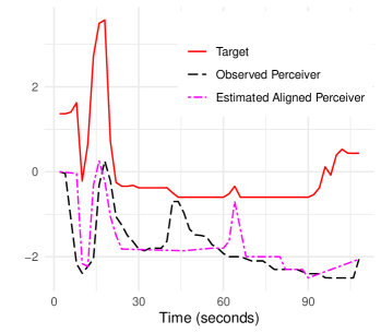
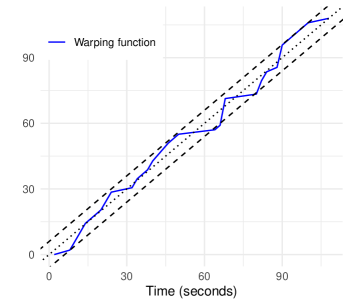
Because the temporal window can vary according to the emotions and the modality (Gunes and Pantic,, 2010; Gunes and Schuller,, 2013), we used three thresholds of , and seconds for EA applications in Section 5. Figure 3(b) shows penalized alignment of the same example presented in Figure 3(a), using an upper limit of warping function differences of six seconds (). Since for unpenalized alignment, penalized alignment shrinks the estimated warping function toward the identity warping function. Consequently, the resulting aligned perceiver sequence does not exhibit peaks or valleys that deviate from the observed perceiver sequence by more than six seconds.
4 Simulation Study
To demonstrate the performance of our functional alignment approach, we conducted a simulation study. It is challenging to use real EA data to evaluate functional alignment methods because perceivers’ responses without misalignment are unknown. However, we can generate perceivers’ responses without phase misalignment, denoted as perceivers’ aligned responses in simulations, and use them to assess the effectiveness of different alignment methods.
4.1 Simulation 1
Let denote the th target function (). We first generate a non-stationary time series for each target by computing the inverse of the lagged differences of a stationary time series that consists of 300 values randomly sampled from the standard normal distribution. Then, we smooth it using the Gaussian kernel smoother with a bandwidth of and record the functional values for 300 evenly-spaced time points (). For each target, we generate perceiver response ratings for , in two steps. In the first step, we generate a set of perceiver’s aligned response , which is the ideal perceiver’s response without misalignment. In the second step, we shift the phase of perceiver function by warping the aligned perceiver function with the warping function that mimics the misalignment patterns observed in real emotion rating data.
Specifically, in the first step, we generate the th aligned perceiver’s response by shifting the phase and changing the amplitude of the th target by ; , , is the one-dimensional Wiener process (i.e., Brownian motion) at time (Mörters and Peres,, 2010), is the Gaussian kernel smoother with bandwidth , and is the non-stationary time series, randomly generated using the same procedure as the target, and smoothed with . Multiplying and adding to the target enables a gradual phase shift and amplitude change and determines the noise level. As a result, each perceiver’s aligned response contains random noise with minor phase misalignment when is close to 0.5 whereas could differ from target when is close to 1.
In the second step, the phase of is shifted by the warping function for , where is the true individual upper limit of the warping amount. The detailed warping function generation algorithm is given in Section S2.1 of the supplementary material. To account for individual warping variations, is randomly generated from the gamma distribution with shape and scale under three sets of parameters, . We denote an observed perceiver response as so the true warping function that recovers the perceiver’s aligned response is the inverse of the warping function used for the phase shift .
We align the observed perceiver response to the target using four methods: 1) no alignment, 2) optimal fixed delay, 3) unpenalized SRVF alignment, and 4) penalized SRVF alignment. Let denote the estimated perceiver response. The no alignment uses the identity warping . The optimal fixed delay finds the optimum amount of delay that achieves the smallest distance between and , where if , if , and otherwise. The warping functions of the unpenalized and penalized SRVF alignments are obtained by solving (2) and (5), respectively. In our simulation, we set the warping limit for alignment to regardless of the true warping limit , to reflect the real-world cases where the true warping limit is unknown.
The objective of the alignment is to recover the perceivers’ aligned responses from , such that the analysis based on the aligned responses, , will be more accurate than that based on the unaligned responses . If the alignment method over-aligns, the aligned response will be too close to the target . On the other hand, will be close to when the alignment method under-aligns. Thus, the optimal approach will have its estimated warping function to be close to the true warping function .
We evaluate how accurately the alignment methods estimate the perceivers’ aligned responses with four metrics. First, we compare the correlations between the perceiver’s aligned response and the estimated perceiver’s response . Under the optimal alignment where , the correlation is expected to be close to 1. Second, we compute the distance between the true and the estimated warping functions , where is the true warping function and is the estimated warping function. The closer gets to zero, the more accurate estimation of the phase shift is. Third, we evaluate the differences between the SRVF representations of the perceiver’s aligned and estimated responses, . A small value of suggests that the amplitude variability between the perceiver’s aligned and estimated responses is small. Lastly, we compute the mean squared error (MSE) between the true and the estimated correlations to the target, . Here, is commonly used metrics for measuring EA, and can be considered as the ideal correlation that the alignment methods aim to achieve.
| Metric | Penalized SRVF | Unpenalized SRVF | Optimal Fixed | No alignment | |
|---|---|---|---|---|---|
| 0.855 (0.157) | 0.798 (0.224) | 0.724 (0.219) | 0.747 (0.194) | ||
| 0.067 (0.034) | 0.098 (0.066) | 0.094 (0.033) | 0.074 (0.028) | ||
| 2.630 (0.726) | 2.743 (0.753) | 3.191 (0.684) | 3.416 (0.736) | ||
| MSE | 0.036 | 0.078 | 0.061 | 0.042 | |
| 0.859 (0.153) | 0.798 (0.221) | 0.724 (0.216) | 0.744 (0.189) | ||
| 0.066 (0.111) | 0.099 (0.124) | 0.095 (0.110) | 0.075 (0.109) | ||
| 2.613 (0.728) | 2.746 (0.751) | 3.192 (0.676) | 3.445 (0.732) | ||
| MSE | 0.035 | 0.078 | 0.061 | 0.041 | |
| 0.864 (0.150) | 0.800 (0.220) | 0.724 (0.214) | 0.744 (0.185) | ||
| 0.064 (0.044) | 0.098 (0.072) | 0.095 (0.041) | 0.074 (0.037) | ||
| 2.589 (0.727) | 2.738 (0.749) | 3.184 (0.670) | 3.454 (0.725) | ||
| MSE | 0.035 | 0.078 | 0.061 | 0.041 |
Table 3 shows the summary of the four metrics for the four alignment methods. The proposed penalized SRVF has demonstrated the best performance in recovering the perceiver’s aligned responses. First, the estimated perceivers’ responses by penalized SRVF have the highest average correlations to perceivers’ aligned responses. Also, the average distance of the proposed penalized SRVF is closest to zero, implying that the proposed method makes the most accurate estimation of the phase shift. Third, the average SRVF distance between the perceiver’s true and aligned responses of the penalized SRVF is the smallest. This suggests that the penalized SRVF makes the least amplitude variability after alignment. Lastly, MSE shows that the penalized SRVF yields the most accurate correlation to the target.
The unpenalized SRVF method produces a less accurate estimate of than the penalized SRVF. Additionally, the variabilities of , , and are the highest among the four methods. This is because unpenalized SRVF tends to over-align the perceiver’s response towards the target . We present the summary of associations between the target and the estimated perceivers’ response of the four alignment methods in Section S2.2 of the supplementary material.
4.2 Simulation 2
We further investigate the robustness of the alignment warping limit, . In practical applications, the precise true warping limit, , is often unknown. Consequently, the alignment warping limit, , must be selected based on approximate prior knowledge, potentially deviating from . In this simulation, data is generated following the same setting in Section 4.1 except that the true warping limit is not randomly generated. We use five different true warping limits while the warping limit for alignment is set to be .
| Metric | Penalized SRVF | Unpenalized SRVF | Optimal Fixed | No alignment | |
|---|---|---|---|---|---|
| 0.891 (0.121) | 0.792 (0.228) | 0.792 (0.181) | 0.850 (0.113) | ||
| 0.053 (0.020) | 0.095 (0.059) | 0.070 (0.021) | 0.049 (0.005) | ||
| 2.505 (0.695) | 2.751 (0.749) | 3.054 (0.676) | 3.148 (0.685) | ||
| 20 | MSE | 0.031 | 0.084 | 0.037 | 0.018 |
| 0.882 (0.134) | 0.791 (0.230) | 0.759 (0.193) | 0.798 (0.146) | ||
| 0.057 (0.023) | 0.098 (0.062) | 0.083 (0.021) | 0.062 (0.006) | ||
| 2.520 (0.718) | 2.753 (0.752) | 3.119 (0.661) | 3.338 (0.703) | ||
| 25 | MSE | 0.033 | 0.085 | 0.048 | 0.027 |
| 0.867 (0.147) | 0.791 (0.228) | 0.724 (0.212) | 0.746 (0.176) | ||
| 0.063 (0.025) | 0.101 (0.065) | 0.095 (0.021) | 0.074 (0.007) | ||
| 2.564 (0.736) | 2.760 (0.750) | 3.175 (0.669) | 3.458 (0.714) | ||
| 30 | MSE | 0.035 | 0.085 | 0.059 | 0.038 |
| 0.833 (0.165) | 0.792 (0.228) | 0.697 (0.225) | 0.700 (0.203) | ||
| 0.075 (0.026) | 0.105 (0.068) | 0.105 (0.020) | 0.086 (0.007) | ||
| 2.747 (0.694) | 2.753 (0.753) | 3.261 (0.660) | 3.532 (0.712) | ||
| 35 | MSE | 0.037 | 0.084 | 0.067 | 0.05 |
| 0.795 (0.183) | 0.790 (0.229) | 0.666 (0.237) | 0.656 (0.224) | ||
| 0.087 (0.025) | 0.110 (0.072) | 0.114 (0.019) | 0.097 (0.008) | ||
| 2.879 (0.680) | 2.760 (0.748) | 3.347 (0.658) | 3.581 (0.711) | ||
| 40 | MSE | 0.041 | 0.085 | 0.075 | 0.063 |
Table 2 summarizes the performance metrics of four alignment methods across five different true warping limits. The penalized SRVF method generally outperforms the other methods. When the true warping limits are smaller than the warping limit for alignment (i.e., ), the no-alignment method performs comparably to penalized SRVF due to small true warping limits. Conversely, when the true warping limits are larger than (i.e., ), some metrics of penalized SRVF get closer to those of unpenalized SRVF, but penalized SRVF still outperforms in most cases. some penalized SRVF metrics approach those of unpenalized SRVF, though penalized SRVF remains superior in most cases. These findings indicate that selecting within a reasonable warping limit range yields robust alignment outcomes for the penalized SRVF method, even when the exact degree of true warping, , is uncertain.
5 Data application
5.1 Study on Social Empathy
In the first data application, we analyzed a dataset from Devlin et al., (2014), which consists of 121 perceivers’ empathy responses of four distinct videos in which the targets discuss emotional events in their lives. The four videos vary in valence (positive or negative) and intensity (high or low), resulting in four heterogeneous videos, including high-positive, low-positive, high-negative, and low-negative. Participants provided continuous 9-point scale ratings of target emotions while watching each video. These perceiver ratings were compared to target self-ratings. Following standard functional data analysis practices (Srivastava and Klassen,, 2016), we preprocessed the data by smoothing target and perceiver ratings using cubic smoothing splines with the default setting of the smooth.spline function in R and interpolating the estimated functions on a 300-point equidistant grid within the observed time interval. The goal of the subsequent analysis is to measure the level of EA for each perceiver.
Figure 2 clearly illustrates the misalignment between perceiver and target ratings. Devlin et al., (2014) did not account for this misalignment, measuring EA as a monotonic transformation of the Pearson correlation between the two rating sequences. We applied both unpenalized and penalized SRVF alignments, as these methods offer more flexible time warping than fixed delay alignment. Here, we present results for the penalized alignment with a threshold of seconds. Results for thresholds of 6 and 10 seconds are included in Section S3.1 of the supplementary material.
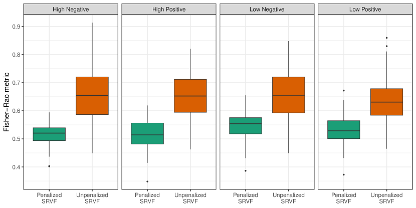
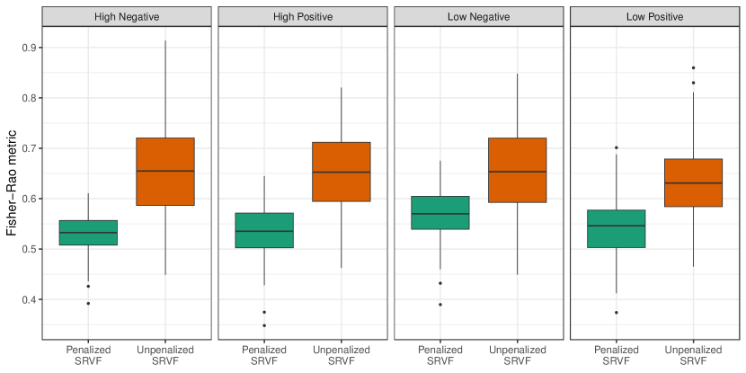
To quantify the degree of warping, we computed the phase distance () between the estimated warping function under each alignment method and the identity warping function for each video. Figure 4 reveals that the unpenalized SRVF alignment consistently produces warping functions farther from the identity function than the penalized SRVF alignment, indicating the latter’s effectiveness in reducing excessive warping.

We subsequently calculated the Pearson correlation between each perceiver’s aligned ratings and the target’s ratings. Unlike the simulation studies, the correlation coefficient between the target () and the aligned perceiver response () is not observable. Instead, we compared these correlations to those obtained without alignment (identity warping), referred to as identity correlations. Notably, about 2% of the cases exhibited negative correlations between perceiver and target ratings under identity warping. As a data pre-processing step, we removed those cases based on the concern that they may exhibit fundamentally different empathy patterns from the general population of perceivers.
Figure 5 presents scatterplots comparing correlations between target and perceiver ratings for pre- and post-aligned data across the four video conditions. The majority of points reside above the 45-degree line, indicating that accounting for misalignment generally increases correlations compared to unadjusted analyses. However, the unpenalized SRVF alignment often inflates correlations considerably, as observed in the simulation results reported in Section S2.2 in the supplementary material. This is most pronounced in the low-positive emotion video group (bottom right panel of Figure 5), where many unpenalized correlations approach one, implying near-perfect empathy for most perceivers, an unrealistic outcome given the video’s low expressiveness. Conversely, for the high-positive video group (top right panel), some unpenalized correlations fall substantially below identity correlations because excessive warping distorted overall function trends.
The proposed penalized SRVF alignment effectively balances the identity correlation and the unpenalized correlation. For low-expressivity videos (bottom row, Figure 5), penalized alignment correlations generally exceed those from no alignment, likely due to increased misalignment challenges under reduced emotional cues. It is also interesting to find that for videos under positive emotion (second column, Figure 5), the correlation with the penalized SRVF alignment has a trivial difference compared with the correlation with no alignment, while for videos under negative emotion (first column, Figure 5), the difference is much bigger. This suggests a stronger time-warping effect for negative emotions, which is consistent with psychological research indicating better recognition of positive emotions (Bandyopadhyay et al.,, 2021).
5.2 Study on Music Empathy
Tabak et al., (2022) conducted an EA study investigating three primary emotions: joy/happiness, sadness, and anger (). For each emotion, three original solo piano pieces () were composed and performed by experienced musicians. These pieces were designed to evoke the target emotions within familiar musical styles (classical, popular, and jazz). Both musicians (as targets) and 123 participants (as perceivers) rated the emotional content of each piece on a 9-point scale. As with the previous dataset, we preprocessed the data by smoothing and interpolating rating functions.
Unlike the correlation-based approach, Tabak et al., (2022) employed a linear mixed-effect model for a more nuanced analysis of EA. This model decomposed perceiver responses into three latent factors: bias, discrimination, and variance. Bias represented the systematic deviation between perceiver and target ratings, while discrimination captured a perceiver’s sensitivity to changes in the target’s expressed emotion. Finally, variance accounted for random noise in perceiver ratings.
Within each group of emotion (), let and be the target and a perceiver’s ratings, respectively, for the th stimulus. Tabak et al., (2022) proposed the following linear mixed-effect model to describe the relationship between and :
| (8) |
where and are the perceiver and target’s respective ratings at the th time point, and is the number of points for the th stimuli. The (fixed) intercept and slope represent a perceiver’s mean bias and discrimination ability across all the stimuli, respectively. The random intercept , random slope , and the random noise are assumed to follow a normal distribution with zero mean and respective variance component and , which represents the variability of bias, discrimination, and random noise across different stimuli. This model treats ratings as discrete points and does not account for potential misalignments between perceiver and target responses.
To address this limitation, we integrated an alignment step into the model framework. Treating the observed ratings as sampled points from corresponding functions, we applied and compared penalized and unpenalized time-warping SRVF alignments to account for potential misalignments. Let be the aligned response with being an estimated warping function from aligning with , we then modeled the following:
| (9) |
where , , and in Model (9) maintain the same interpretations as in Model (8). We fitted Model (9) for each perceiver and primary emotion. Using the lme4 package in R (Bates et al.,, 2015), we employed restricted maximum likelihood estimation to obtain parameter estimates and best linear unbiased predictions (BLUPs) of random effects and for . To assess the impact of time warping, we compared parameter estimates under no alignment (i.e., ), the unpenalized SRVF (), and the penalized SRVF alignment (, setting the penalty threshold at seconds for the penalized alignment. Results for 6- and 10-second thresholds are provided in Section S3.2 of the supplementary material.
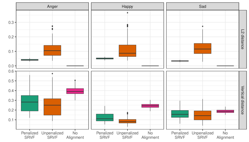
To assess model fit, we computed two metrics: average warping and average goodness of fit across all tasks. The first metric, average Fisher-Rao distance, quantifies the mean warping magnitude relative to the identity warping: . A higher indicates greater warping. The second metric measures the vertical distance between the estimated aligned response function and the fitted value function. Specifically, letting , this vertical distance is calculated to be the distance between the estimated aligned response and the fitted value function , i.e., , where a lower value signifies a better model fit.
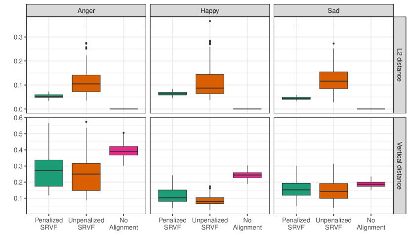
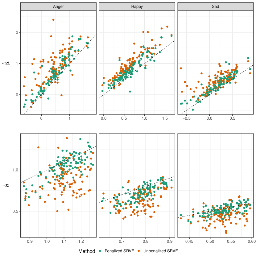
Figure 6 reveals that the no-alignment model exhibits inferior fit compared to the other two approaches. This underscores the importance of addressing misalignment between perceiver and target ratings to prevent model underfitting. Similar to our simulation findings, the unpenalized alignment demonstrates overfitting, sacrificing model fit for excessive warping. In contrast, the penalized alignment method provides a balance between these extremes, enhancing model fit while mitigating overfitting through judicious penalty application.
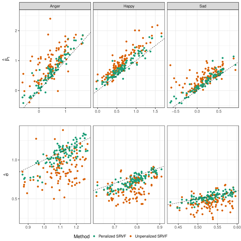
Figure 7 compares parameter estimates (aligned vs. unaligned) for the fixed effect discrimination () and random noise standard deviation () across emotion groups. Both alignment methods reduce compared to the no-alignment condition, as misaligned rating sequences inflate random noise. Aligned responses exhibit stronger associations with target responses, decreasing unexplained variability. While both alignments reduce , the unpenalized alignment achieves a more substantial reduction due to over-alignment.
Regarding the fixed effect discrimination (), unaligned responses can be viewed in a certain way as aligned responses contaminated by measurement error. By correcting for misalignment, the attenuation bias in estimates is reduced, leading to increased values as depicted in Figure 7’s first row. However, the excessive warping associated with unpenalized alignment amplifies this effect.
6 Discussion
Misalignment is a well-established phenomenon in emotional perception research, yet there remains a dearth of rigorous statistical methods to correct it. Neglecting misalignment in EA data analysis can lead to significantly biased results. Conventional approaches, such as accounting for fixed delays in responses, oversimplify the complex nature of misalignment. This study introduces a novel, flexible approach using penalized warping functions to address the multifaceted nature of misalignment in cognitive perception studies.
While warping functions have been widely employed to correct misalignment in fields like physics and biology, where objective benchmarks exist, their application to the abstract and subjective domain of human perception is relatively unexplored. The challenges inherent in accurately measuring perceptual constructs have often led to the neglect of misalignment in cognitive research. This study represents a significant step toward addressing this critical issue.
Our proposed penalized alignment approach offers several advantages. 1) Individualized adjustments: It tailors alignment to unique patterns of misalignment for each participant. 2) Prevention of over-alignment: It incorporates a natural constraint on the extent of allowable warping. 3) Simplicity and interpretability: It eliminates the need for parameter tuning and provides clear results. By providing a flexible and robust method for correcting misalignment, our approach empowers researchers to conduct more accurate downstream EA analyses, such as correlational studies and complex linear mixed models.
Future research could focus on several key areas. One potential direction is to model the similarity of warping functions of the same individual across different stimuli by introducing random effects. Another area of interest could be to develop a new EA alignment method by incorporating additional data, such as the functional magnetic resonance imaging (fMRI) blood-oxygen-level-dependent (BOLD) signals of targets and perceivers during rating assessments, which could help detect true emotional changes.
References
- Bandyopadhyay et al., (2021) Bandyopadhyay, A., Sarkar, S., Mukherjee, A., Bhattacherjee, S., and Basu, S. (2021). Identifying emotional facial expressions in practice: A study on medical students. Indian Journal of Psychological Medicine, 43(1):51–57.
- Bates et al., (2015) Bates, D., Mächler, M., Bolker, B., and Walker, S. (2015). Fitting linear mixed-effects models using lme4. Journal of Statistical Software, 67(1):1–48.
- Berndt and Clifford, (1994) Berndt, D. J. and Clifford, J. (1994). Using dynamic time warping to find patterns in time series. In Proceedings of the 3rd international conference on knowledge discovery and data mining, pages 359–370.
- Bharath et al., (2018) Bharath, K., Kurtek, S., Rao, A., and Baladandayuthapani, V. (2018). Radiologic image-based statistical shape analysis of brain tumours. Journal of the Royal Statistical Society. Series C, Applied statistics, 67(5):1357.
- Blair, (2005) Blair, R. (2005). Responding to the emotions of others: dissociating forms of empathy through the study of typical and psychiatric populations. Consciousness and cognition, 14(4):698–718.
- De Waal, (2008) De Waal, F. B. (2008). Putting the altruism back into altruism: The evolution of empathy. Annu. Rev. Psychol., 59:279–300.
- Devlin et al., (2014) Devlin, H. C., Zaki, J., Ong, D. C., and Gruber, J. (2014). Not as good as you think? trait positive emotion is associated with increased self-reported empathy but decreased empathic performance. PloS one, 9(10):e110470.
- Ekman, (1992) Ekman, P. (1992). An argument for basic emotions. Cognition & emotion, 6(3-4):169–200.
- Gunes and Pantic, (2010) Gunes, H. and Pantic, M. (2010). Automatic, dimensional and continuous emotion recognition. International Journal of Synthetic Emotions (IJSE), 1(1):68–99.
- Gunes and Schuller, (2013) Gunes, H. and Schuller, B. (2013). Categorical and dimensional affect analysis in continuous input: Current trends and future directions. Image and Vision Computing, 31(2):120–136.
- Guo et al., (2022) Guo, X., Wu, W., and Srivastava, A. (2022). Data-driven, soft alignment of functional data using shapes and landmarks. arXiv preprint arXiv:2203.14810.
- Huang et al., (2015) Huang, Z., Dang, T., Cummins, N., Stasak, B., Le, P., Sethu, V., and Epps, J. (2015). An investigation of annotation delay compensation and output-associative fusion for multimodal continuous emotion prediction. In Proceedings of the 5th International Workshop on Audio/Visual Emotion Challenge, pages 41–48.
- Jospe et al., (2020) Jospe, K., Genzer, S., klein Selle, N., Ong, D., Zaki, J., and Perry, A. (2020). The contribution of linguistic and visual cues to physiological synchrony and empathic accuracy. Cortex, 132:296–308.
- Khorram et al., (2019) Khorram, S., McInnis, M. G., and Provost, E. M. (2019). Jointly aligning and predicting continuous emotion annotations. IEEE Transactions on Affective Computing, 12(4):1069–1083.
- Kneip et al., (2000) Kneip, A., Li, X., MacGibbon, K., and Ramsay, J. (2000). Curve registration by local regression. Canadian Journal of Statistics, 28(1):19–29.
- Kokoszka and Reimherr, (2017) Kokoszka, P. and Reimherr, M. (2017). Introduction to functional data analysis. Chapman and Hall/CRC.
- Laga et al., (2014) Laga, H., Kurtek, S., Srivastava, A., and Miklavcic, S. J. (2014). Landmark-free statistical analysis of the shape of plant leaves. Journal of theoretical biology, 363:41–52.
- Lee et al., (2011) Lee, J., Zaki, J., Harvey, P.-O., Ochsner, K., and Green, M. (2011). Schizophrenia patients are impaired in empathic accuracy. Psychological medicine, 41(11):2297–2304.
- Levenson, (1988) Levenson, R. W. (1988). Emotion and the autonomic nervous system: A prospectus for research on autonomic specificity. Social psychophysiology and emotion: Theory and clinical applications, pages 17–42.
- Mackes et al., (2018) Mackes, N. K., Golm, D., O’Daly, O. G., Sarkar, S., Sonuga-Barke, E. J., Fairchild, G., and Mehta, M. A. (2018). Tracking emotions in the brain–revisiting the empathic accuracy task. NeuroImage, 178:677–686.
- Mariooryad and Busso, (2014) Mariooryad, S. and Busso, C. (2014). Correcting time-continuous emotional labels by modeling the reaction lag of evaluators. IEEE Transactions on Affective Computing, 6(2):97–108.
- Marron et al., (2015) Marron, J. S., Ramsay, J. O., Sangalli, L. M., and Srivastava, A. (2015). Functional data analysis of amplitude and phase variation. Statistical Science, pages 468–484.
- Mitchell et al., (2022) Mitchell, E. G., Dryden, I. L., Fallaize, C. J., Andersen, R., Bradley, A. V., Large, D. J., and Sowter, A. (2022). Object oriented data analysis of surface motion time series in peatland landscapes. arXiv preprint arXiv:2209.14187.
- Mörters and Peres, (2010) Mörters, P. and Peres, Y. (2010). Brownian motion, volume 30. Cambridge University Press.
- Nicolle et al., (2012) Nicolle, J., Rapp, V., Bailly, K., Prevost, L., and Chetouani, M. (2012). Robust continuous prediction of human emotions using multiscale dynamic cues. In Proceedings of the 14th ACM international conference on Multimodal interaction, pages 501–508.
- Ramsay and Li, (1998) Ramsay, J. O. and Li, X. (1998). Curve registration. Journal of the Royal Statistical Society: Series B (Statistical Methodology), 60(2):351–363.
- Ramsay and Silverman, (2005) Ramsay, J. O. and Silverman, B. W. (2005). Functional Data Analysis. Springer.
- Ringeval et al., (2015) Ringeval, F., Eyben, F., Kroupi, E., Yuce, A., Thiran, J.-P., Ebrahimi, T., Lalanne, D., and Schuller, B. (2015). Prediction of asynchronous dimensional emotion ratings from audiovisual and physiological data. Pattern Recognition Letters, 66:22–30.
- Sakoe and Chiba, (1978) Sakoe, H. and Chiba, S. (1978). Dynamic programming algorithm optimization for spoken word recognition. IEEE transactions on acoustics, speech, and signal processing, 26(1):43–49.
- Scherer, (2003) Scherer, K. R. (2003). Vocal communication of emotion: A review of research paradigms. Speech communication, 40(1-2):227–256.
- Schweinle et al., (2002) Schweinle, W. E., Ickes, W., and Bernstein, I. H. (2002). Emphatic inaccuracy in husband to wife aggression: The overattribution bias. Personal Relationships, 9(2):141–158.
- Sened et al., (2017) Sened, H., Lavidor, M., Lazarus, G., Bar-Kalifa, E., Rafaeli, E., and Ickes, W. (2017). Empathic accuracy and relationship satisfaction: A meta-analytic review. Journal of Family Psychology, 31(6):742.
- Srivastava et al., (2007) Srivastava, A., Jermyn, I., and Joshi, S. (2007). Riemannian analysis of probability density functions with applications in vision. In 2007 IEEE Conference on Computer Vision and Pattern Recognition, pages 1–8. IEEE.
- Srivastava and Klassen, (2016) Srivastava, A. and Klassen, E. P. (2016). Functional and shape data analysis. Springer.
- Srivastava et al., (2011) Srivastava, A., Wu, W., Kurtek, S., Klassen, E., and Marron, J. S. (2011). Registration of functional data using fisher-rao metric. arXiv preprint arXiv:1103.3817.
- Su et al., (2014) Su, J., Kurtek, S., Klassen, E., and Srivastava, A. (2014). Statistical analysis of trajectories on riemannian manifolds: bird migration, hurricane tracking and video surveillance.
- Tabak et al., (2022) Tabak, B. A., Wallmark, Z., Nghiem, L. H., Alvi, T., Sunahara, C. S., Lee, J., and Cao, J. (2022). Initial evidence for a relation between behaviorally assessed empathic accuracy and affect sharing for people and music. Emotion.
- Tucker, (2023) Tucker, J. D. (2023). fdasrvf: Elastic Functional Data Analysis. R package version 2.0.2.
- Tucker et al., (2014) Tucker, J. D., Wu, W., and Srivastava, A. (2014). Analysis of proteomics data: Phase amplitude separation using an extended fisher-rao metric.
- Wallace et al., (2014) Wallace, W. E., Srivastava, A., Telu, K. H., and Simón-Manso, Y. (2014). Pairwise alignment of chromatograms using an extended fisher–rao metric. Analytica Chimica Acta, 841:10–16.
- Wang and Gasser, (1997) Wang, K. and Gasser, T. (1997). Alignment of curves by dynamic time warping. The Annals of Statistics, 25(3):1251–1276.
- Wu and Srivastava, (2011) Wu, W. and Srivastava, A. (2011). An information-geometric framework for statistical inferences in the neural spike train space. Journal of Computational Neuroscience, 31:725–748.
- Wu and Srivastava, (2014) Wu, W. and Srivastava, A. (2014). Analysis of spike train data: Alignment and comparisons using the extended fisher-rao metric.
- Xie et al., (2017) Xie, W., Kurtek, S., Bharath, K., and Sun, Y. (2017). A geometric approach to visualization of variability in functional data. Journal of the American Statistical Association, 112(519):979–993.
- Zaki et al., (2008) Zaki, J., Bolger, N., and Ochsner, K. (2008). It takes two: The interpersonal nature of empathic accuracy. Psychological science, 19(4):399–404.
- Zaki et al., (2009) Zaki, J., Bolger, N., and Ochsner, K. (2009). Unpacking the informational bases of empathic accuracy. Emotion, 9(4):478.
- Zhao et al., (2020) Zhao, W., Xu, Z., Li, W., and Wu, W. (2020). Modeling and analyzing neural signals with phase variability using fisher-rao registration. Journal of Neuroscience Methods, 346:108954.
Supplementary Materials
Appendix A Proof of Lemma 3.1
Proof.
Let be the set of warping functions under penalized warping of (5), , , , is invertible, and are smooth, . By representing as its SRVF , the space maps to . Here, and . Because is a subset of the positive orthant of the unit Hilbert sphere , also is a subset of . Therefore, the SRVF of warping functions from the penalized SRVF are the elements of a unit Hilbert sphere, and their distance is the arc-length distance. It can be approximated by . ∎
Appendix B Supplements to Simulation Study
B.1 Generation of Warping Functions
Given a value of , the warping function is generated in the following steps:
-
•
Generate the first random intervals and such that and
-
•
In the first random interval , the warping limit is achieved by shifting the identity warping function up by , i.e for .
-
•
In the second random interval , the warping limit is achieved by shifting the identity warping function down by , i.e for .
-
•
Linear interpolation is conducted for constructing the warping function in the intervals , and . We note that the condition in the first step is needed to ensure the constructed function is increasing in the interval .
B.2 Association between Target and Estimated Response
We compare the association between the target and the estimated perceivers’ responses using two metrics: 1) the difference in correlations between the target and the estimated perceiver’s response and the aligned and estimated perceiver’s responses , where and and 2) the difference in SRVF distances of the target and estimated perceivers’ responses and the aligned and estimated perceivers’ responses , where and . The large positive values of and the large negative values of suggest that the estimated responses are over-aligned to targets. On the other hand, the large negative values of and the large positive values of imply the estimated responses are under-aligned compared to the aligned perceiver’s response.
| Metric | Penalized SRVF | Unpenalized SRVF | Optimal Fixed | No alignment | |
|---|---|---|---|---|---|
| 0.111 (0.154) | 0.191 (0.205) | -0.044 (0.242) | -0.080 (0.188) | ||
| -1.363 (0.493) | -1.660 (0.497) | 0.312 (0.627) | 0.710 (0.705) | ||
| 0.112 (0.150) | 0.191 (0.204) | -0.043 (0.242) | -0.080 (0.187) | ||
| -1.376 (0.481) | -1.664 (0.497) | 0.309 (0.626) | 0.712 (0.709) | ||
| 0.113 (0.150) | 0.190 (0.204) | -0.045 (0.243) | -0.080 (0.187) | ||
| -1.379 (0.471) | -1.660 (0.497) | 0.311 (0.626) | 0.717 (0.710) |
Table 3 summarizes and of the four alignment methods. The unpenalized SRVF method overestimates the correlation, it also has the smallest SRVF distance to the target, resulting from over-alignment. The no-alignment and the fixed-alignment methods underestimate the correlation and carry considerably large SRVF distance to the target, resulting from under-alignment.
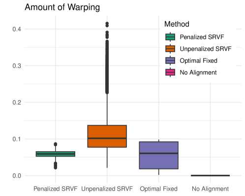
The unpenalized SRVF also makes the largest amount of phase alignment. Figure 8 shows boxplots of 50,000 phase alignment amounts of four alignment methods, measured by the differences between the estimated warping function from the identity warping function, . The mean phase alignment is highest with the unpenalized SRVF method (0.113), lowest with the optimal fixed method (0.055), and the proposed penalized SRVF method falls in between these two (0.059).
Appendix C Supplementary Plots for Data Applications
C.1 Data application: Social empathy
This section contains additional results for the first data application, including the estimates of the amount of warping and correlation between the aligned perceivers and the targets under different thresholds.
| Video | Metric | No alignment | Unpenalized SRVF | Penalized SRVF | ||
|---|---|---|---|---|---|---|
| Correlation | 0.51 (0.14) | 0.68 (0.11) | 0.58 (0.15) | 0.59 (0.16) | 0.58 (0.17) | |
| Low Negative | Amount of Warping | 0.00 (0.00) | 0.66 (0.09) | 0.50 (0.05) | 0.55 (0.05) | 0.57 (0.05) |
| Correlation | 0.73 (0.20) | 0.85 (0.13) | 0.75 (0.19) | 0.75 (0.19) | 0.75 (0.19) | |
| High Negative | Amount of Warping | 0.00 (0.00) | 0.66 (0.10) | 0.50 (0.03) | 0.52 (0.04) | 0.53 (0.04) |
| Correlation | 0.89 (0.15) | 0.85 (0.26) | 0.91 (0.15) | 0.91 (0.15) | 0.91 (0.15) | |
| High Positive | Amount of Warping | 0.00 (0.00) | 0.65 (0.08) | 0.49 (0.05) | 0.52 (0.05) | 0.53 (0.05) |
| Correlation | 0.46 (0.28) | 0.68 (0.44) | 0.50 (0.29) | 0.52 (0.30) | 0.54 (0.31) | |
| Low Positive | Amount of Warping | 0.00 (0.00) | 0.64 (0.07) | 0.49 (0.04) | 0.53 (0.05) | 0.54 (0.05) |


C.2 Data application: Music empathy
This section contains additional results for the first data application, including the estimates of the amount of warping and all parameters under different thresholds.

| Parameter | No alignment | Unpenalized SRVF | Penalized SRVF | ||||
|---|---|---|---|---|---|---|---|
| Anger | Amount of warping | 0.00 (0.00) | 0.63 (0.09) | 0.51 (0.03) | 0.53 (0.03) | 0.54 (0.04) | |
| Vertical distance | 1.19 (0.24) | 0.80 (0.33) | 1.10 (0.33) | 1.06 (0.32) | 1.01 (0.31) | ||
| 0.52 (3.75) | -1.32 (4.02) | -0.26 (4.12) | -0.33 (4.11) | -0.51 (4.08) | |||
| 0.64 (0.81) | 1.08 (0.85) | 0.83 (0.89) | 0.85 (0.89) | 0.89 (0.87) | |||
| 1.09 (0.12) | 0.88 (0.19) | 1.04 (0.17) | 1.02 (0.17) | 1.00 (0.16) | |||
| 3.58 (3.10) | 3.63 (3.06) | 3.94 (3.40) | 3.92 (3.24) | 3.98 (3.32) | |||
| 0.81 (0.64) | 0.84 (0.62) | 0.89 (0.69) | 0.89 (0.66) | 0.91 (0.67) | |||
| Happy | Amount of warping | 0.00 (0.00) | 0.64 (0.10) | 0.52 (0.04) | 0.55 (0.05) | 0.56 (0.05) | |
| Vertical distance | 0.60 (0.10) | 0.42 (0.16) | 0.53 (0.13) | 0.52 (0.14) | 0.51 (0.14) | ||
| 2.08 (2.95) | -0.27 (4.28) | 1.22 (2.99) | 1.03 (2.99) | 0.92 (3.07) | |||
| 0.74 (0.53) | 1.13 (0.80) | 0.87 (0.55) | 0.90 (0.55) | 0.91 (0.56) | |||
| 0.77 (0.07) | 0.64 (0.12) | 0.72 (0.09) | 0.71 (0.10) | 0.71 (0.10) | |||
| 2.16 (1.89) | 3.02 (2.87) | 2.17 (1.78) | 2.26 (1.79) | 2.43 (2.00) | |||
| 0.34 (0.35) | 0.50 (0.59) | 0.35 (0.33) | 0.37 (0.32) | 0.39 (0.37) | |||
| Sad | Amount of warping | 0.00 (0.00) | 0.63 (0.09) | 0.50 (0.04) | 0.52 (0.04) | 0.53 (0.04) | |
| Vertical distance | 0.28 (0.04) | 0.21 (0.08) | 0.27 (0.06) | 0.26 (0.07) | 0.26 (0.07) | ||
| 3.10 (1.91) | 2.13 (3.40) | 2.61 (2.00) | 2.47 (2.04) | 2.35 (2.08) | |||
| 0.21 (0.41) | 0.43 (0.69) | 0.32 (0.42) | 0.36 (0.43) | 0.38 (0.44) | |||
| 0.53 (0.04) | 0.45 (0.09) | 0.52 (0.06) | 0.51 (0.06) | 0.50 (0.07) | |||
| 2.49 (2.51) | 2.85 (5.17) | 2.60 (3.01) | 2.62 (3.00) | 2.70 (3.21) | |||
| 0.49 (0.50) | 0.56 (1.04) | 0.51 (0.61) | 0.51 (0.61) | 0.53 (0.65) | |||