Graffin: Stand for Tails in Imbalanced Node Classification

Abstract

Graph representation learning (GRL) models have succeeded in many scenarios. Real-world graphs have imbalanced distribution, such as node labels and degrees, which leaves a critical challenge to GRL. Imbalanced inputs can lead to imbalanced outputs. However, most existing works ignore it and assume that the distribution of input graphs is balanced, which cannot align with real situations, resulting in worse model performance on tail data. The domination of head data makes tail data underrepresented when training graph neural networks (GNNs). Thus, we propose Graffin, a pluggable tail data augmentation module, to address the above issues. Inspired by recurrent neural networks (RNNs), Graffin flows head features into tail data through graph serialization techniques to alleviate the imbalance of tail representation. The local and global structures are fused to form the node representation under the combined effect of neighborhood and sequence information, which enriches the semantics of tail data. We validate the performance of Graffin on four real-world datasets in node classification tasks. Results show that Graffin can improve the adaptation to tail data without significantly degrading the overall model performance.

Introduction

Graph representation learning (GRL) models have succeeded in many scenarios, like recommendations (Han et al. 2024), bioinformatics (Hu et al. 2023), etc. Node classification is one of the typical tasks (Zhang et al. 2023b; Zhao, Zhang, and Wang 2024; Achten et al. 2024), where the goal is to learn a classifier predicting the ground labels of nodes. Researchers have explored graph neural networks (GNNs) in this domain, proposing amounts of foundation models (Kipf and Welling 2017; Velickovic et al. 2018; Zhao, Zhang, and Wang 2021). Existing works achieve noteworthy performance, most assuming that the distribution is balanced.

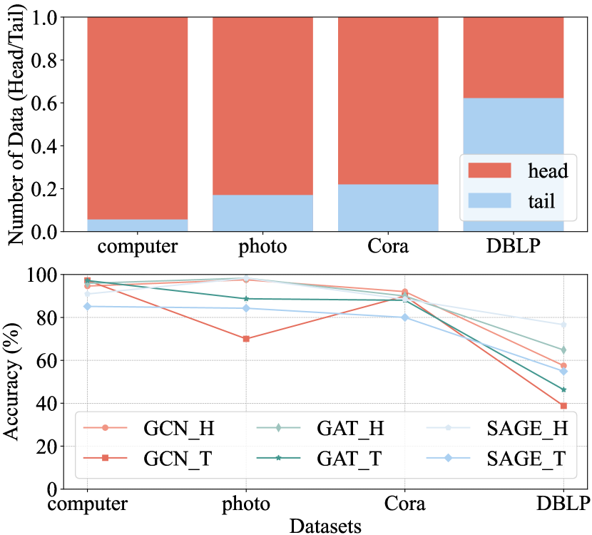
Figure 1: Imbalanced characteristics in node classification tasks. Top: Imbalanced distribution of node classes. Bottom: Imbalanced classification performance, where H and T denote the results of head and tail data.

However, real-world graphs usually have imbalanced distribution, such as node labels and degrees, which leaves a critical challenge to GRL. For example, in Figure 1, we illustrate the imbalanced statistics of four real-world datasets. Each bar shows the proportion of the tail data (blue) to the head data (red). The tails are far less than the heads. In the worst case, the tail data is only 5.6% of the head. Though DBLP has a relatively well-balanced situation, with fewer classes having less gap between each other, tails are still 38% less than head data. Imbalanced inputs can lead to imbalanced outputs. We further train three vanilla models to test the classification performance, and the results show that models perform better on the head. We take photo as an example, with 1941 head data and 331 tail data. The average model performances are $98.06\pm 0.36$ and $81.01\pm 7.97$, respectively. Head data are better represented and more robust, having a superiority of about 17.05%. The domination of head data makes tail data underrepresented and turbulent, resulting in worse tail classification accuracy.

This phenomenon brings out an interesting topic of enhancing the performance of GRL models, especially for tail data, in an imbalanced setting. Researchers have worked on imbalanced graph learning (IGL) (Zhao, Zhang, and Wang 2021; Park, Song, and Yang 2022) for a long time. They improve the tail data performance or balance heads and tails through sampling or generating strategies. However, these approaches change the original graph distribution and may introduce noise due to virtual nodes and edges. We focus on building a structure-oriented strategy with only original graph structural information to alleviate the noise caused by sampling. Some works (Yun et al. 2022; Wang et al. 2022) have tried augmentation approaches, using specific knowledge or information to enrich the tails. It suffers from obtaining complicated structures like subgraphs with unbearable cost.

Moreover, existing works consider the imbalance under a single scenario like node class or degree. Nevertheless, sources causing imbalance are various and intertwined in real-world cases (Xu et al. 2024). For example, ordinary users on social networks account for the vast majority (a large sample number in a particular label), but each of them owns poor interests (low degree). On the contrary, a small portion of core users can absorb several times the number of connections other users have. It urges the proposal of a mixed framework that combines various imbalance factors.

Therefore, in this paper, we proposed a novel pluggable module, Graffin, to stand for tails and improve their performance in imbalanced node classification. Our goal is to enhance the adaptation to tail data without significantly degrading the overall model performance. We introduce an information augmentation strategy instead of sampling that changes the original distribution. We flow more context to tail data via the graph serialization technique, orientating to the graph structure without generating new nodes and edges. Next, we design a mixup of local and global structures, which enriches the semantics of tail data to the same level as the heads. It is a combination framework of GNN and RNN, where the former aggregates 1-hop neighbors through the message-passing mechanism to represent local features, and the latter learns sequential information from heads to tails as a sample of global features. Most importantly, the information flow of the graph sequence is in serialization order, jumping out of the limitation of topological structures. It could learn latent features from long-distance node pairs. Diversity in both features balances the fusion, forming the final node representation.

In summary, our main contributions are as follows:

• As far as we know, we are the first to integrate sequential information to graph data under an imbalanced scenario. We flow head features into tail data through graph serialization techniques instead of sampling to alleviate the imbalance of tail representation. It orientates toward the original graphs without changing the distribution or generating synthetic nodes.

• We propose a novel pluggable module, Graffin, leveraging sequential semantics via RNNs. We fuse the local and global structures to form the node representation under the combined effect of neighborhood and sequence information, which enriches the semantics of tail data.

• We validate the performance of Graffin on four real-world datasets in node classification tasks. Results show that Graffin can improve the adaptation to tail data without significantly degrading the overall model performance. Moreover, other classes, not only tails, can benefit from the sequence.

Related Work

Imbalanced Graph Learning

Imbalanced graph learning (IGL) (Zeng et al. 2023; Liu et al. 2023a; Xu et al. 2024) derives from traditional imbalanced learning works and is more complicated since graphs have various sources of imbalance, such as classes, degrees, etc. The data-level algorithm is one of the mainstream countermeasures for solving imbalanced problems. Inspired by SMOTE (Chawla et al. 2002), GraphSMOTE (Zhao, Zhang, and Wang 2021) synthesizes nodes for tail classes, oversampling until balanced. It constructs new edges between existing nodes and synthetic samples. GraphENS (Park, Song, and Yang 2022) takes a further step, generating the neighbors of tail data rather than only themselves. It builds subgraphs of tails to provide more semantics. CM-GCL (Qian et al. 2022) puts imbalanced learning into a contrastive learning paradigm, developing a co-modality framework to generate contrastive pairs automatically. However, virtual nodes and edges sampled and generated in the works above change the original graph distribution, leading to extra noise.

Despite the re-balancing approaches of the GraphSMOTE branch, other works (Wu et al. 2021; Yun et al. 2022; Wang et al. 2022) aim to enrich tail data with extra information augmentation. GraphMixup (Wu et al. 2021), inspired by Mixup, designs multiple augmentation strategies from various aspects. It can adaptively change the upsampling ratio of tail data with the power of reinforcement learning. G2GNN (Wang et al. 2022) adds a graph-of-graph view based on kernel similarity to obtain high-level supernode features on graph tasks. Meanwhile, ImGCL (Zeng et al. 2023) also tries contrastive learning, leveraging the progressively balanced sampling method with pseudo-labels. These works use extra information augmentation, keeping alignment with the original graph distribution. But they suffer to compute more complex structures such as subgraphs, graph-of-graphs, etc.

For more details about IGL, we suggest reading the surveys (Liu et al. 2023b; Ju et al. 2024).

Graph Sequence Modeling

GNNs can handle neighbors well but fail to capture long-distance node interactions due to their message-passing mechanism. However, models such as recurrent neural networks (RNNs) (Chung et al. 2014) are powerful in dealing with sequential data. They can learn rich representation and remember historical information in a long sequence. The non-serializable property is one of the vital resistances of applying these models to graphs. Though some works attempt to combine graphs and sequences, most of which are rich in sequential semantics, such as time series in temporal graphs (Zhang et al. 2023a) and SMILES sequence in molecular graphs (Hu et al. 2023). Few methods are ready for general graphs to capture latent features behind sequences. Recently, researchers have aimed at linear-time sequence modeling methods. Many designs arise, such as selective state spaces (Gu, Goel, and Ré 2022), real-gated linear recurrent units (De et al. 2024), etc. It allows rethinking the combination of graphs and sequences.

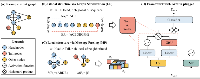
Figure 2: Overview of the proposed Graffin method. (A) Example input graph with imbalanced node class distribution. (B) Sequential global structure via graph serialization (GS). (C) 1-hop local structure via message passing (MP) neural networks. (D) Example framework with exchangeable MP with Graffin plugged.

Preliminaries

Attributed Graph.

An attributed graph can form as $\mathcal{G}=\{\mathcal{V},\mathcal{E},\mathcal{X},\Phi,\mathcal{Y}\}$, where $\mathcal{V}=\{v_{1},...,v_{N}\}$ and $\mathcal{E}=\{e_{ij}|v_{i},v_{j}\in\mathcal{V}\}$ represent the set of nodes and edges, and $\mathcal{X}\in\mathbb{R}^{N\times D}$ denotes the graph attributes with $D$ dimensions. The function $\Phi:\mathcal{V}\rightarrow\mathcal{Y}$ maps a node $v\in\mathcal{V}$ to its corresponding label $y\in\mathcal{Y}$. We use $\mathcal{A}\in\{0,1\}^{N\times N}$ to represent the adjacency matrix, where $\mathcal{A}[i,j]=1$ if $e_{ij}\in\mathcal{E}$.

Imbalance Ratio.

Imbalanced data distribution occurs frequently due to the complex characteristics of graphs. In this paper, we aim at node class imbalance. We evaluate it via a node class imbalance ratio, $R_{imb}$. Mathematically, for a graph $\mathcal{G}$ with $K$ independent node classes, where $\mathcal{Y}=\bigcup_{1\leq i\leq K}\mathcal{Y}_{i}$, the imbalance ratio is defined as

$$R_{imb}=\frac{|\mathcal{Y}_{\max}|}{|\mathcal{Y}_{\min}|},$$ (1)

where $|\mathcal{Y}_{\min}|$ and $|\mathcal{Y}_{\max}|$ denote the number of tail and head data. $R_{imb}\geq 1$, and the larger the number, the more imbalanced the datasets. It is an ideal balance when $R_{imb}=1$.

Problem Formulation.

Node classification is one of the most vital applications in GNNs, aiming at mapping all nodes into several classes. Given a graph $\mathcal{G}=\{\mathcal{V},\mathcal{E},\mathcal{X},\Phi,\mathcal{Y}\}$, the goal is to learn a new mapping function $\bar{\Phi}:\mathcal{V}\rightarrow\bar{\mathcal{Y}}$, predicting ground truths $\mathcal{Y}$ correctly.

Graffin: The Proposed Framework

Figure 2 shows the overview framework of our proposed method, Graffin. Inspired by RNNs, we flow head features into tail data through graph serialization techniques to alleviate the imbalance of tail representation. Heads own more neighborhoods than tails. Thus, tails need to grab more in sequence. We fuse the local and global structures to form the node representation under the combined effect of neighborhood and sequence information, which enriches the semantics of tail data.

Graph Serialization

Global Structure via Graph Serialization.

One of the most popular methods for alleviating the imbalance is re-balancing (Zhao, Zhang, and Wang 2021; Park, Song, and Yang 2022). However, these approaches change the original distribution of nodes. It may introduce additional noise and can’t align with reality. With this in mind, we hope to find an information augmentation strategy instead of breaking the original distribution. Some intuitive works (Yun et al. 2022; Wang et al. 2022) have focused on it. However, they keep the balancing phase without being oriented to the original graph and have far more complex extra information (e.g., subgraphs) to compute.

Inspired by the concept of meta-path (Dong, Chawla, and Swami 2017), we serialize graph data to get global structures hiding in the graph sequence. Given a node set $\mathcal{V}$ and its attribute $\mathcal{X}$, we have the graph serialization (GS) block as

$$(\mathcal{V}^{\prime},\mathcal{X}^{\prime})=\textit{GS}^{\sigma}(\mathcal{V},\mathcal{X}),$$ (2)

where $\mathcal{V}^{\prime}$ is the indices of rearranged nodes, and $\mathcal{X}^{\prime}$ is the new stacked attributes. $\sigma$ denotes the serialization strategy GS picks. We default it to node degrees according to the intertwined characteristics of class and structure (Xu et al. 2024).

Countering traditional ideas that more important nodes should have more context (Wang et al. 2024), we compute the sequence through GS to enrich the tails. In other words, tail data should seize a longer node list. In sequential data, each node only updates based on previous nodes from hidden states due to the nature of sequences. For example, as shown in Figure 2(B), we serialize the input graph in a descending degree order, where $\forall v_{i},v_{j}\in\mathcal{V}$, if $i<j$, then $\sigma_{i}>\sigma_{j}$. Let $\textit{GS}_{v}$ be the historical set node $v$ could see. The last tail data $H$, having $N-1$ (self-omitted) previous nodes as context, is far more than the head $C$, which has only one node $A$ in the set. In usual cases, we define a global structure enriching ratio,

$$R_{g}=\frac{|\bar{\textit{GS}}_{head}|}{|\bar{\textit{GS}}_{tail}|},$$ (3)

to express the improvement of the tail context. Head data have a relatively small amount of context, approximating $|\mathcal{Y}_{\max}|/2$, while tails are at the end of the sequence, having almost $N$ nodes selected in the hidden state. To make a simplification, we set $R_{g}\approx R_{imb}/N$.

Graffin: Control Information Flows.

The intuition behind Graffin is simple. RNN’s autoregressive ability can easily capture long-distance node interactions. After acquiring the graph sequence, it learns global structures by serialization order, jumping out of the limitations of edges. For the last tail data, we show the information flow following GRU (Chung et al. 2014):

$$h_{tail}=g\odot h_{pre}+(1-g)\odot s_{tail},$$ (4)

where $g$ denotes a learnable recurrence gate, $pre$ and $s$ are the previous node of the tail, and the hidden state of the tail, respectively.

Note that pre is the predecessor of the last tail data by serialization order. It drops the topological restriction, finding long-distance node pairs in different ego networks and memorizing their representations. Those historical nodes build the context of the last tail data, fused in the hidden state:

$$s_{tail}=\textit{tanh}(h_{tail}W_{tail}+(s_{pre}\odot r)W_{pre}),$$ (5)

where $r$ is another learnable gate function used for updating, $W$ is the corresponding weighted matrix, and tanh is the hyperbolic tangent function. Both gate functions follow the same format as

$$f(h_{tail})=\delta(h_{tail}W_{tail}^{f}+h_{pre}W_{pre}^{f}),$$ (6)

where $\delta$ refers to the activation function such as sigmoid.

This behavior could learn two similar nodes not directly connected with edges. For example, as shown in Figures 2(A) and (B), $F$ rather than $G$ is the previous node of the tail data $H$ in the graph sequence. That is because $F$ has a nearer relationship with $H$ defined by $\sigma$ (both have one node degree), where $|\sigma_{F}-\sigma_{H}|\leq|\sigma_{G}-\sigma_{H}|$. In the same way, $A$ is the predecessor of the head data $C$, w.r.t. $B$ and $D$, due to the overlap in the neighborhoods $\mathcal{N}_{C}=\{BDE\}\subseteq\mathcal{N}_{A}$ and outer linkages with node $E$, which is not head data.

Therefore, we design our Graffin module following Griffin (De et al. 2024). It takes the normalized graph sequence as the input and separates two branches. The first branch is a plain linear layer with GeLU as the activation, keeping the original node features:

$$\mathcal{T}_{1}=\textit{GeLU}(linear(\mathcal{X^{\prime}})).$$ (7)

The second branch applies an RNN-based core (e.g., GRU) to control the information flowing from heads to tails:

$$\mathcal{T}_{2}=\textit{GRU}(linear(\mathcal{X^{\prime}})).$$ (8)

Ultimately, we merge two branches to get the final representation of global sequential structures:

$$\mathcal{H}_{g}=\mathcal{T}_{1}\odot\mathcal{T}_{2},$$ (9)

which is a fusion of node representation $\mathcal{T}_{1}$ and sequential information $\mathcal{T}_{2}$. The former ensures that self-features do not drop while the latter learns the graph sequence, avoiding over-smooth or indistinguishable.

Structure Mixing

Local Structure via Message Passing.

Noteworthyly, GNNs achieve venerable impacts on node representations through their message passing (MP) techniques (Kipf and Welling 2017). We utilize MP to aggregate 1-hop neighborhoods, forming local structures of each node. In general, for a node $v$, a possible layer of MP is

$$h_{v}=\textit{aggr}_{u\in\mathcal{N}(v)}(h_{u}),$$ (10)

where $\mathcal{N}(v)$ represents the neighbor nodes of $v$, and aggr can be any aggregating functions (e.g., sum or average neighborhood features). As shown in Figure 2(C), for an imbalanced graph, head data own richer representations than tails due to various local structures of neighbors. We use $\textit{MP}_{v}=\{u|u\in\mathcal{N}(v)\}$ to represent the neighbors of node $v$. There are more nodes in the neighbors of the head data $C$ than the tail $H$, where $|\textit{MP}_{C}|=4\gg|\textit{MP}_{A}|$. The more nodes the neighborhood has, the more representations the message-passing aggregates. Therefore, it can define the imbalance in the local structure via the local ratio

$$R_{l}=\frac{|\bar{\textit{MP}}_{head}|}{|\bar{\textit{MP}}_{tail}|}.$$ (11)

Since tail data often have a relatively small number of neighbors, we can approximate $R_{l}$ with $N$ and $R_{imb}$, where $R_{l}\approx N/R_{imb}$.

Why Mixing Works.

From the above discussion, we define two ratios, $R_{g}$ and $R_{l}$, where $R_{g}R_{l}\approx 1$. It describes why combining local and global structures can enrich the representation of tail data. $R_{g}$ flows the entire node set to tail data, showing the absolute position, while $R_{l}$ keeps the original neighborhood information as a relative one. Thus, the fusion may balance the semantics, especially for tails, to the same level as heads.

We take one-hot encoding and sum aggregation as an example. Here, $\mathcal{H}_{l}$ shows the 1-hop neighbor structures, and $\mathcal{H}_{g}$ gives the number of each class in the context. Since $|\textit{MP}_{head}|\gg|\textit{MP}_{tail}|$, heads limit the feature spaces via a shorter context $\textit{GS}_{head}$, which nearly equals learning representation with only head data. Meanwhile, we let $|\textit{GS}_{tail}|\approx N\gg|\textit{GS}_{head}|$, which accumulates node features in a subnetwork directed by serialization order rather than edges, in other words, message passing. Thus, it covers a range of nodes with similar characteristics defined by $\sigma$ without losing its individuality when classifying tail data.

Framework with Graffin plugged.

Figure 2(D) shows how Graffin works when plugged. There are two main streams of structural information flow. Given a graph attribute matrix $\mathcal{X}\in\mathbb{R}^{N\times D}$, we keep local structures $\mathcal{H}_{l}$ of 1-hop neighbors through MP, using ReLU as the activation:

$$\mathcal{H}_{l}=\textit{ReLU}(\textit{MP}(\mathcal{X})),$$ (12)

where MP can be any message-passing framework aggregating neighbors in the same format as Equation 10.

Meanwhile, we leverage GS to rearrange the node semantics as Equation 2 and Graffin to control the information flows from heads to tails according to Equations 7- 9. After that, we have global structures $\mathcal{H}_{g}$ of sequence standing for tail data:

$$\mathcal{H}_{g}=\textit{Graffin}(\textit{GS}(\mathcal{X})).$$ (13)

Next, we fuse two parts using Hadamard Product to form the final node representation $\mathcal{H}_{f}$ under the combined effect of neighborhood and sequence information:

$$\mathcal{H}_{f}=\mathcal{H}_{l}\odot\mathcal{H}_{g}.$$ (14)

According to Equation 9, it is a three-part mixup: initial node representation, local structure via MP, and global structure via GS. All of them are original-graph-oriented with easy access.

Finally, we feed $\mathcal{H}_{f}$ to a single linear classifier to compute the label predictions $\bar{\mathcal{Y}}\in\mathbb{R}^{N\times K}$ with an example negative log likelihood loss:

$$loss=-\frac{1}{N}\sum_{i=1}^{N}(y_{i}\log\bar{y}_{i}+(1-y_{i})\log(1-\bar{y}_{i})).$$ (15)

In summary, Algorithm 1 shows the pseudocode of Graffin.

Algorithm 1 Graffin: The Proposed Framework

Input: the input graph $\mathcal{G}=\{\mathcal{V},\mathcal{E},\mathcal{X},\Phi,\mathcal{Y}\}$;
Output: the final node representation $\mathcal{H}_{f}$;

1:  // GS Phase

2:  Compute $\mathcal{V}^{\prime}$ and $\mathcal{X}^{\prime}$ according to Equation 2;

3:  while not converged or not exceeded epochs do

4:     Normalize $\mathcal{X}^{\prime}$;

5:     Compute $\mathcal{T}_{1}$ and $\mathcal{T}_{2}$ according to Equations 7 and  8;

6:     Compute $\mathcal{H}_{g}$ according to Equation 9;

7:     // MP Phase

8:     Compute $\mathcal{H}_{l}$ according to Equation 12;

9:     // Fusion Phase

10:     Rearrange $\mathcal{H}_{g}$ from $\mathcal{V}^{\prime}$ to $\mathcal{V}$;

11:     Compute $\mathcal{H}_{f}$ according to Equation 14;

12:     Update the model according to Equation 15;

13:  end while

14:  return  $\mathcal{H}_{f}$

Experiments

Datasets.

We use four widely used datasets from real-world scenarios, including Amazon computers, Amazon photo, Cora, and DBLP. Table 1 shows the statistics of them. Among datasets, DBLP constructs a heterogeneous graph. We simplify it where nodes are from two types: Author and Paper, and edges from Author-Paper. Then, we apply the classification task on nodes of type Author.

Baselines.

We consider six pluggable baseline models from two categories: (1) Vanilla GRL models: GCN (Kipf and Welling 2017), GAT (Velickovic et al. 2018), and GraphSAGE (SAGE) (Hamilton, Ying, and Leskovec 2017). (2) SOTA models for imbalanced learning: GraphSMOTE (SMO) (Zhao, Zhang, and Wang 2021), GraphENS (ENS) (Park, Song, and Yang 2022), and ImbGNN (Imb) (Xu et al. 2024). We further introduce SOTA models in Appendix B.

Evaluation Metrics.

Following previous work (Zhao, Zhang, and Wang 2021) on evaluating imbalanced node classification, we set three measurements: overall accuracy (ALL), average AUC-ROC (A.R.), and macro F1-score (F1). Dominated by head data, ALL may give a limited evaluation of tail data. A.R. gives a robust view of classification performance, not relying on a specific threshold, while F1 considers all classes by calculating the harmonic mean of Precision and Recall. Furthermore, we also report tail data accuracy (LOW), computing all tail examples at once. All metrics can thoroughly reflect the performance of models on tail data.

Implementation Details.

We run all experiments on a 64-bit machine with NVIDIA GeForce RTX 3050 OEM GPU, 8GB. As for all vanilla GRL models, we apply a single layer and linear as the core and classifier. We use Adam (Kingma and Ba 2015) as the optimizer, initializing the learning rate to 0.01, with a weight decay 5e-4. As for other imbalanced learning SOTA models, we reproduce their open-source codes and keep the settings with them. SMO uses SAGE as the core layer and adds mean absolute error with square error as the final loss function. ENS uses GCN instead, training with cross-entropy. Though Imb is for imbalanced graph-level tasks, it treats each graph as a supernode to apply high-level node classification. Thus, it is easy to transfer from graph-level tasks to node-level. We utilize a stacked 5-layer GIN (Xu et al. 2019) to encode, a 2-layer MLP to classify, and the same target loss as Graffin. Codes are available in Appendix C. To make a fair comparison, we repeat all experiments five times to report the average with the same training epoch of 200.

Datasets	# N	# D	# Cl	$R_{imb}$
Amazon computers	13,752	767	10	17.73
Amazon photo	7,650	745	8	5.86
Cora	2,708	1,433	7	4.54
DBLP	18,385	334	4	1.61

Table 1: The statistics of datasets. # N, # D, and # Cl show the number of nodes, features, and node classes. $R_{imb}$ indicates the node class imbalanced rate of each dataset.

Main Results on Node Classification

Dataset	Meas.	GCN	+ Gf	GAT	+ Gf	SAGE	+ Gf	SMO	+ Gf	ENS	+ Gf	Imb	+ Gf
computers	ALL	$89.9^{1.0}$	$87.7^{0.9}$	$89.5^{3.0}$	$\textbf{89.5}^{1.2}$	$88.8^{1.5}$	$87.2^{0.7}$	$52.9^{2.8}$	$\textbf{63.4}^{3.2}$	$83.7^{0.8}$	$\textbf{85.6}^{0.2}$	$43.2^{1.5}$	$\textbf{86.0}^{0.5}$
	LOW	$96.2^{0.7}$	$\textbf{98.0}^{0.7}$	$96.8^{1.8}$	$\textbf{98.7}^{0.8}$	$91.8^{5.2}$	$\textbf{97.3}^{1.7}$	$4.7^{2.2}$	$\textbf{40.4}^{11.1}$	$95.0^{0.6}$	$\textbf{96.0}^{0.4}$	$0.0^{0.0}$	$\textbf{98.4}^{0.4}$
	A.R.	$99.5^{0.1}$	$\textbf{99.9}^{0.0}$	$99.7^{0.3}$	$\textbf{99.9}^{0.0}$	$99.5^{0.2}$	$\textbf{99.9}^{0.0}$	$89.5^{0.7}$	$\textbf{94.6}^{0.9}$	$99.4^{0.0}$	$\textbf{99.7}^{0.0}$	$74.3^{2.4}$	$\textbf{99.9}^{0.0}$
	F1	$88.0^{3.3}$	$\textbf{98.0}^{0.1}$	$94.5^{3.2}$	$\textbf{98.4}^{0.3}$	$88.0^{5.0}$	$\textbf{98.0}^{0.3}$	$48.7^{3.0}$	$\textbf{62.1}^{4.0}$	$82.4^{0.8}$	$\textbf{83.2}^{0.3}$	$13.4^{2.6}$	$\textbf{97.6}^{0.2}$
photo	ALL	$93.5^{1.2}$	$92.6^{0.5}$	$93.0^{1.2}$	$\textbf{94.4}^{0.4}$	$92.7^{3.8}$	$\textbf{92.8}^{1.0}$	$69.8^{2.0}$	$\textbf{80.4}^{3.4}$	$92.4^{0.2}$	$92.3^{0.2}$	$32.3^{8.6}$	$\textbf{91.7}^{0.9}$
	LOW	$71.7^{10.3}$	$\textbf{95.0}^{1.0}$	$88.9^{5.7}$	$\textbf{95.7}^{2.2}$	$79.0^{15.5}$	$\textbf{92.1}^{1.2}$	$6.8^{3.8}$	$\textbf{53.2}^{9.1}$	$86.2^{0.5}$	$\textbf{93.6}^{0.6}$	$0.0^{0.0}$	$\textbf{94.0}^{1.5}$
	A.R.	$99.6^{0.2}$	$\textbf{99.9}^{0.0}$	$99.6^{0.2}$	$\textbf{99.9}^{0.1}$	$99.7^{0.2}$	$\textbf{99.9}^{0.0}$	$94.3^{0.2}$	$\textbf{95.6}^{0.9}$	$98.9^{0.0}$	$\textbf{99.8}^{0.0}$	$70.2^{8.9}$	$\textbf{99.9}^{0.0}$
	F1	$93.5^{1.4}$	$\textbf{98.2}^{0.2}$	$96.1^{2.1}$	$\textbf{98.7}^{0.1}$	$92.8^{1.0}$	$\textbf{98.0}^{0.2}$	$66.4^{1.8}$	$\textbf{80.2}^{3.6}$	$90.5^{0.3}$	$\textbf{92.0}^{0.2}$	$16.9^{6.6}$	$\textbf{98.0}^{0.2}$
Cora	ALL	$84.2^{1.1}$	$83.7^{0.9}$	$79.9^{2.1}$	$\textbf{83.0}^{1.1}$	$79.6^{0.8}$	$\textbf{80.7}^{0.7}$	$45.8^{3.9}$	$\textbf{53.3}^{2.6}$	$84.7^{0.2}$	$83.6^{0.4}$	$32.3^{8.6}$	$\textbf{91.7}^{0.9}$
	LOW	$89.2^{2.1}$	$\textbf{89.3}^{2.8}$	$83.1^{2.5}$	$\textbf{86.0}^{3.2}$	$83.5^{2.5}$	$\textbf{84.2}^{2.3}$	$21.8^{4.8}$	$\textbf{49.8}^{9.6}$	$90.7^{0.7}$	$\textbf{91.1}^{0.2}$	$0.0^{0.0}$	$\textbf{94.0}^{1.5}$
	A.R.	$98.7^{0.1}$	$\textbf{98.7}^{0.1}$	$97.7^{0.6}$	$\textbf{98.4}^{0.2}$	$98.5^{0.1}$	$\textbf{98.6}^{0.1}$	$81.1^{2.5}$	$\textbf{83.3}^{1.4}$	$98.9^{0.0}$	$\textbf{99.1}^{0.0}$	$70.2^{8.9}$	$\textbf{99.9}^{0.0}$
	F1	$90.3^{0.6}$	$\textbf{90.4}^{0.5}$	$88.1^{0.9}$	$\textbf{89.6}^{0.2}$	$88.1^{0.6}$	$\textbf{88.7}^{0.4}$	$44.3^{4.8}$	$\textbf{51.9}^{3.6}$	$83.8^{0.2}$	$83.0^{0.3}$	$16.9^{6.6}$	$\textbf{98.0}^{0.2}$
DBLP	ALL	$47.7^{1.1}$	$\textbf{78.3}^{0.3}$	$58.0^{2.0}$	$\textbf{77.9}^{0.2}$	$67.0^{1.2}$	$\textbf{78.7}^{0.3}$	$30.0^{0.6}$	$\textbf{30.3}^{0.9}$	$46.1^{0.3}$	$\textbf{77.9}^{0.9}$	$27.6^{3.0}$	$\textbf{77.4}^{0.3}$
	LOW	$37.2^{1.5}$	$\textbf{72.1}^{1.5}$	$49.4^{2.8}$	$\textbf{71.0}^{2.0}$	$61.2^{8.4}$	$\textbf{70.0}^{1.9}$	$28.1^{8.1}$	$\textbf{38.8}^{7.6}$	$28.7^{2.0}$	$\textbf{65.2}^{1.6}$	$22.8^{5.0}$	$\textbf{70.0}^{2.9}$
	A.R.	$75.4^{0.5}$	$\textbf{93.1}^{0.2}$	$81.5^{1.9}$	$\textbf{93.8}^{0.1}$	$88.9^{0.6}$	$\textbf{92.7}^{0.3}$	$54.5^{2.2}$	$\textbf{58.4}^{4.2}$	$70.5^{0.2}$	$\textbf{93.1}^{0.4}$	$54.9^{2.7}$	$\textbf{94.0}^{0.1}$
	F1	$53.3^{4.1}$	$\textbf{79.5}^{0.2}$	$61.0^{1.9}$	$\textbf{79.0}^{0.2}$	$69.4^{1.0}$	$\textbf{79.7}^{0.2}$	$25.0^{1.5}$	$\textbf{27.3}^{1.6}$	$43.7^{0.4}$	$\textbf{76.8}^{0.8}$	$28.8^{4.3}$	$\textbf{78.6}^{0.3}$

Table 2: Performance comparison on node classification with baselines. We report mean scores ($mean$) and standard deviations ($dev$) in the format $mean^{dev}$. +Gf means the base model plugged with Graffin.

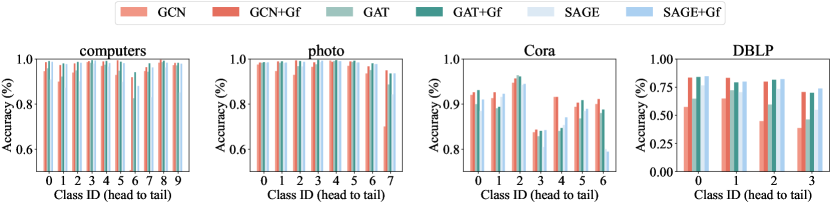
Figure 3: All classes accuracy w/o Graffin plugged. The class indexes are sorted from head to tail according to the number of nodes in each class.

Table 2 shows the main results of the node classification task. All baseline models achieve noteworthy tail data performance gains with Graffin plugged. From a dataset perspective, all baseline models perform poorly on DBLP. Since we simplify it with only two types of nodes remaining, models can’t capture enough features to learn the graph. However, with Graffin plugged in, all model performances improve by a huge step. Graph sequence can dig out the latent structural information, finding long-distance node interactions to enrich tail representations.

Graffin successfully increases the accuracy of tail data, LOW, which is the initial purpose of our model. The best case occurs when GCN plugs Graffin, which has an average LOW increase of 15.03% among all four datasets. We focus carefully on the balanced performance between classes, resulting in higher A.R. and F1 scores. It shows that other nodes can benefit from the graph sequence, not only heads and tails. Thus, the overall accuracy among all classes, ACC, also gains a lot, with only a few baseline models slightly dropping on one or two datasets. We will show more details about the model performance of all classes later.

Surprisingly, Imb shows a competitive node classification ability with Graffin plugged, though it is for graph-level tasks at the beginning. Imb goes from barely recognizing tail data (0% LOW ACC for most datasets) to a classification level of around 90%, illustrating a significant impact for the tails. To sum up, Graffin can improve the adaptation to tail data without significantly degrading the overall model performance.

All Classes Analysis

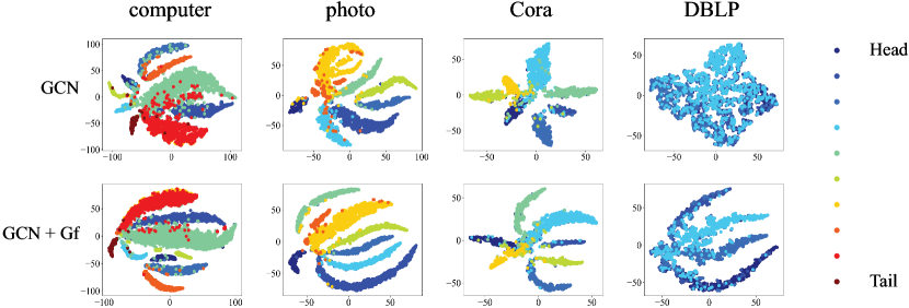
Figure 4: t-SNE visualization of GCN and GCN with Graffin (GCN+Gf) on all four datasets. Each color represents one node class from head data to tail data.

We further analyze the accuracy of all node classes in Figure 3 to show how Graffin stands for tails in imbalanced node classification tasks. In general, Graffin achieves its goal of improving the classification accuracy for tail data (the last bar in each subplot). Cora has the least significant average growth of 0.44%, while DBLP shows the best case of 24.88%. Head data also have a considerable increase. Although these nodes memorize shorter contexts in the sequence, they can still learn richer semantics due to their enormous base number.

As a matter of fact, except for heads and tails, we find other nodes benefit from the graph sequence, too. An arbitrary node $v$ can learn more or less sequential information according to the serialization strategy, which complements the topological local neighbors. Not all classes take advantage of the graph sequence. The worst case is not precisely the tails. For example, the worst performance occurring in computer is 59.86% for class 6 (93.19% for tails), with a quantity ratio of 487:291. That could explain why Graffin decays overall performances in some cases.

Ablation on Graph Serialization Strategy

Dataset	Type	computer	photo	Cora	DBLP
GCN	degree	$98.03$	$98.23$	$90.38$	$79.48$
	eigen	-$0.05$	-$0.03$	-$0.42$	-$0.03$
	id	-$0.08$	-$0.03$	-$0.77$	-$0.74$
GAT	degree	$98.37$	$98.73$	$89.62$	$79.01$
	eigen	-$0.00$	-$0.01$	-$0.22$	+$0.21$
	id	-$0.22$	-$0.43$	-$0.36$	-$0.59$
SAGE	degree	$97.95$	$97.97$	$88.73$	$79.72$
	eigen	-$0.24$	+$0.02$	-$0.68$	-$0.81$
	id	-$0.25$	-$0.74$	-$1.42$	-$0.95$

Table 3: Ablation studies on different graph serialization strategies. We report relative F1 scores to consider precisions and recalls comprehensively.

Except for node degrees, we also try two other serialization strategies: node eigenvector centrality and the default order of node ID. The former computes $\lambda x^{T}=x^{T}A$ associated with the eigenvalue $\lambda$. For node $v$, $\sigma=\sum_{u\rightarrow v}\sigma/\lambda$. The latter is approximately equal to a basic random order. Table 3 illustrates the relative F1 scores of the ablation studies. We set the node degree strategy as a baseline, where the negative number denotes the decline, and a positive number underlined denotes a better case. Results show that the node degree strategy picked achieves higher and more stable scores. The other two approaches are slightly weaker but still competitive concerning vanilla models. The eigenvector is better than the node degree in GAT on DBLP (+0.21%) and SAGE on photo (+0.02%). The order of node ID, random order in other words, also provides considerable structural features within sequences. The above conclusions reveal the effectiveness of the graph sequence in node representation, especially those breaking the graph topology, which can learn representations of nodes similar but not connected.

Visualization

To clearly illustrate the power of Graffin, we design visualization experiments via t-SNE (van der Maaten and Hinton 2008). We take GCN as an example due to the paper length limit. Results of the other two vanilla models, GAT and SAGE, can be found in Appendix A. As shown in Figure 4, vanilla GCN can not distinguish tail data well, which mixes the representations of tails with other classes. This phenomenon is more apparent in DBLP, where class representations couple tightly, resulting in underrepresented tail data. GCN+Gf has more distinct boundaries among different classes. With the help of sequential information, the representation space of each class shows the same form of fluid, which could match and evaluate with multiple linear. Note there is a clustering center connected to each fluid where the hard samples fall. GCN+Gf effectively reduces the scale of this area and the number of nodes in it.

Conclusion

In this paper, we aim to improve tail data performance in imbalanced node classification tasks without significantly corrupting the overall. We propose a novel pluggable module, Graffin, enhancing topological semantics through graph sequences. Graffin flows head features into tail data according to graph serialization order and learns the features along the sequence via RNNs to alleviate the imbalance of tail representation. We fuse local and global structures to build a thorough view of neighbors and graph sequences. We conduct the plug-play manner in six baseline models on four real-world datasets to demonstrate the effectiveness of Graffin. The experimental results show that Graffin successfully adapts to tail data without significantly corrupting the overall model performance.

References

- Achten et al. (2024) Achten, S.; Tonin, F.; Patrinos, P.; and Suykens, J. A. K. 2024. Unsupervised Neighborhood Propagation Kernel Layers for Semi-supervised Node Classification. In Thirty-Eighth AAAI Conference on Artificial Intelligence, AAAI 2024, 10766–10774.
- Chawla et al. (2002) Chawla, N. V.; Bowyer, K. W.; Hall, L. O.; and Kegelmeyer, W. P. 2002. SMOTE: Synthetic Minority Over-sampling Technique. J. Artif. Intell. Res., 16: 321–357.
- Chung et al. (2014) Chung, J.; Gülçehre, Ç.; Cho, K.; and Bengio, Y. 2014. Empirical Evaluation of Gated Recurrent Neural Networks on Sequence Modeling. CoRR, abs/1412.3555.
- De et al. (2024) De, S.; Smith, S. L.; Fernando, A.; Botev, A.; Muraru, G.; Gu, A.; Haroun, R.; Berrada, L.; Chen, Y.; Srinivasan, S.; Desjardins, G.; Doucet, A.; Budden, D.; Teh, Y. W.; Pascanu, R.; de Freitas, N.; and Gulcehre, C. 2024. Griffin: Mixing Gated Linear Recurrences with Local Attention for Efficient Language Models. CoRR, abs/2402.19427.
- Dong, Chawla, and Swami (2017) Dong, Y.; Chawla, N. V.; and Swami, A. 2017. metapath2vec: Scalable Representation Learning for Heterogeneous Networks. In Proceedings of the 23rd ACM SIGKDD International Conference on Knowledge Discovery and Data Mining, 135–144.
- Gu, Goel, and Ré (2022) Gu, A.; Goel, K.; and Ré, C. 2022. Efficiently Modeling Long Sequences with Structured State Spaces. In The Tenth International Conference on Learning Representations, ICLR 2022, Virtual Event, April 25-29, 2022. OpenReview.net.
- Hamilton, Ying, and Leskovec (2017) Hamilton, W. L.; Ying, Z.; and Leskovec, J. 2017. Inductive Representation Learning on Large Graphs. In Advances in Neural Information Processing Systems 30: Annual Conference on Neural Information Processing Systems 2017, 1024–1034.
- Han et al. (2024) Han, Z.; Chen, C.; Zheng, X.; Zhang, L.; and Li, Y. 2024. Hypergraph Convolutional Network for User-Oriented Fairness in Recommender Systems. In Proceedings of the 47th International ACM SIGIR Conference on Research and Development in Information Retrieval, SIGIR 2024, 903–913.
- Hu et al. (2023) Hu, H.; Jiang, Y.; Yang, Y.; and Chen, J. X. 2023. Enhanced Template-Free Reaction Prediction with Molecular Graphs and Sequence-based Data Augmentation. In Proceedings of the 32nd ACM International Conference on Information and Knowledge Management, CIKM 2023, 813–822.
- Ju et al. (2024) Ju, W.; Yi, S.; Wang, Y.; Xiao, Z.; Mao, Z.; Li, H.; Gu, Y.; Qin, Y.; Yin, N.; Wang, S.; Liu, X.; Luo, X.; Yu, P. S.; and Zhang, M. 2024. A Survey of Graph Neural Networks in Real world: Imbalance, Noise, Privacy and OOD Challenges. CoRR, abs/2403.04468.
- Kingma and Ba (2015) Kingma, D. P.; and Ba, J. 2015. Adam: A Method for Stochastic Optimization. In 3rd International Conference on Learning Representations, ICLR 2015.
- Kipf and Welling (2017) Kipf, T. N.; and Welling, M. 2017. Semi-Supervised Classification with Graph Convolutional Networks. In 5th International Conference on Learning Representations, ICLR 2017.
- Liu et al. (2023a) Liu, Y.; Gao, Z.; Liu, X.; Luo, P.; Yang, Y.; and Xiong, H. 2023a. QTIAH-GNN: Quantity and Topology Imbalance-aware Heterogeneous Graph Neural Network for Bankruptcy Prediction. In Proceedings of the 29th ACM SIGKDD Conference on Knowledge Discovery and Data Mining, KDD 2023, 1572–1582.
- Liu et al. (2023b) Liu, Z.; Li, Y.; Chen, N.; Wang, Q.; Hooi, B.; and He, B. 2023b. A Survey of Imbalanced Learning on Graphs: Problems, Techniques, and Future Directions. CoRR, abs/2308.13821.
- Park, Song, and Yang (2022) Park, J.; Song, J.; and Yang, E. 2022. GraphENS: Neighbor-Aware Ego Network Synthesis for Class-Imbalanced Node Classification. In The Tenth International Conference on Learning Representations, ICLR 2022.
- Qian et al. (2022) Qian, Y.; Zhang, C.; Zhang, Y.; Wen, Q.; Ye, Y.; and Zhang, C. 2022. Co-Modality Graph Contrastive Learning for Imbalanced Node Classification. In Advances in Neural Information Processing Systems 35: Annual Conference on Neural Information Processing Systems 2022, NeurIPS 2022.
- van der Maaten and Hinton (2008) van der Maaten, L.; and Hinton, G. 2008. Visualizing Data using t-SNE. Journal of Machine Learning Research, 9(86): 2579–2605.
- Velickovic et al. (2018) Velickovic, P.; Cucurull, G.; Casanova, A.; Romero, A.; Liò, P.; and Bengio, Y. 2018. Graph Attention Networks. In 6th International Conference on Learning Representations, ICLR 2018.
- Wang et al. (2024) Wang, C.; Tsepa, O.; Ma, J.; and Wang, B. 2024. Graph-Mamba: Towards Long-Range Graph Sequence Modeling with Selective State Spaces. CoRR, abs/2402.00789.
- Wang et al. (2022) Wang, Y.; Zhao, Y.; Shah, N.; and Derr, T. 2022. Imbalanced Graph Classification via Graph-of-Graph Neural Networks. In Proceedings of the 31st ACM International Conference on Information & Knowledge Management, 2067–2076.
- Wu et al. (2021) Wu, L.; Lin, H.; Gao, Z.; Tan, C.; and Li, S. Z. 2021. GraphMixup: Improving Class-Imbalanced Node Classification on Graphs by Self-supervised Context Prediction. CoRR, abs/2106.11133.
- Xu et al. (2019) Xu, K.; Hu, W.; Leskovec, J.; and Jegelka, S. 2019. How Powerful are Graph Neural Networks? In 7th International Conference on Learning Representations, ICLR 2019.
- Xu et al. (2024) Xu, W.; Wang, P.; Zhao, Z.; Wang, B.; Wang, X.; and Wang, Y. 2024. When Imbalance Meets Imbalance: Structure-driven Learning for Imbalanced Graph Classification. In Proceedings of the ACM on Web Conference 2024, WWW 2024, 905–913.
- Yun et al. (2022) Yun, S.; Kim, K.; Yoon, K.; and Park, C. 2022. LTE4G: Long-Tail Experts for Graph Neural Networks. In Proceedings of the 31st ACM International Conference on Information & Knowledge Management, 2434–2443.
- Zeng et al. (2023) Zeng, L.; Li, L.; Gao, Z.; Zhao, P.; and Li, J. 2023. ImGCL: Revisiting Graph Contrastive Learning on Imbalanced Node Classification. In Thirty-Seventh AAAI Conference on Artificial Intelligence, AAAI 2023, 11138–11146.
- Zhang et al. (2023a) Zhang, H.; Han, X.; Xiao, X.; and Bai, J. 2023a. Time-aware Graph Structure Learning via Sequence Prediction on Temporal Graphs. In Proceedings of the 32nd ACM International Conference on Information and Knowledge Management, CIKM 2023, 3288–3297.
- Zhang et al. (2023b) Zhang, L.; Wang, S.; Liu, J.; Chang, X.; Lin, Q.; Wu, Y.; and Zheng, Q. 2023b. MuL-GRN: Multi-Level Graph Relation Network for Few-Shot Node Classification. IEEE Trans. Knowl. Data Eng., 35(6): 6085–6098.
- Zhao, Zhang, and Wang (2021) Zhao, T.; Zhang, X.; and Wang, S. 2021. GraphSMOTE: Imbalanced Node Classification on Graphs with Graph Neural Networks. In WSDM ’21, The Fourteenth ACM International Conference on Web Search and Data Mining, 833–841.
- Zhao, Zhang, and Wang (2024) Zhao, T.; Zhang, X.; and Wang, S. 2024. Disambiguated Node Classification with Graph Neural Networks. In Proceedings of the ACM on Web Conference 2024, WWW 2024, 914–923.