Turning Water to Wine With Polar Impostorons
Abstract
A surprising result from the theory of quantum control is the degree to which the properties of a physical system can be manipulated. Both atomic and many-body solid state models admit the possibility of creating a ‘driven imposter’, in which the optical response of one material mimics that of a dynamically distinct system. Here we apply these techniques to polarons in polar liquids. Such quasiparticles describe solvated electrons interacting with many-body degrees of freedom of their environment. The polaron frequency, which depends on the electron concentration in the liquid, is controlled with a pump field, rendering the polaron frequency of three different liquids identical. The experiments demonstrate the feasibility of ‘polar impostorons’, a so far purely theoretical phenomenon.
Introduction: Over the previous century, the fundamental principles governing physical systems have (at least in experimentally accessible regimes) been comprehensively uncovered. With a firm grasp of quantum dynamics in hand, a natural question becomes how microscopic behaviour might be exploited. In the present computational age, the dominating preoccupation has centred on how physical systems might themselves be forced to compute. The deep links between physical and informational dynamics [1, 2] means that the control of the former represents a route to mastery of the latter. Examples of this premise abound, where quantum control techniques can be employed in the development of variational quantum algorithms [3], combinatorial optimisation [4], and single-atom computation [5]. More broadly, while quantum control has applications in both information processing [6] and quantum technologies in general [7], it also enables investigations of a more fundamental nature. In particular, quantum control is a tool by which the ultimate limits of the malleability and manipulability of matter can be probed.
One particularly fruitful approach through which questions of this nature can be answered is quantum tracking control [8, 9, 10]. This technique seeks to calculate the driving field required such that the trajectory of some observable expectation conforms to a prespecified “track” [11]. When used in combination with other techniques [12, 13, 14], tracking control has successfully been implemented in a variety of contexts including for atomic [15], molecular [16, 17, 18] and solid-state systems [19, 20, 21].
In the case of these latter systems, microscopic models of strongly-interacting systems make explicit the large degree to which the response of driven systems can be tailored [20]. In particular, they demonstrate a number of intriguing (and potentially exploitable) phenomena. This includes the existence of “twinning fields”, a driving field which elicits an identical response from two dynamically distinct materials [22], and the non-uniqueness of driving fields in generating a given response [23]. Most suggestively, when an observable is a nonlinear function of driving, it is possible to create “driven imposters” where a given system’s response can be tailored to mimic that of an entirely different material [19]. This naturally presents an opportunity in both materials science and chemistry to use simpler and cheaper compounds in combination with driving to obtain some desired property that would otherwise be absent [24, 25, 26, 27, 28].
It is in this final possibility that tracking control has its most romantic potential application - the realisation of the alchemical dream of making lead look like gold. This objective is however also where the limitations of tracking control models considered to this point reveal themselves. In particular, to derive the driving fields necessary to induce whatever behaviour is desired from a system, a microscopic model linking driving field to observable is required. This together with the fact that these solutions for tracking tend to require broad-band control fields [20] have hampered experimental validation of the technique. This naturally raises the question of whether these drawbacks might be circumvented by applying the methodology of tracking control to models more tightly bound to observable behaviour in the laboratory.
This paper answers this question positively, with a novel application of tracking control techniques to an experimental scenario. We focus on manipulating the behavior of polarons – quasiparticles formed through electron-phonon interactions in polar liquids. The models describing the polaronic response are shown to admit the possibility of “polar impostorons” - where distinct liquids may be engineered to exhibit synchronized polaron frequencies. From this, it is possible to demonstrate experimentally the existence of said polar impostorons. Rather than making lead look like gold, polar impostorons allow us to perform the rather more biblical trick of giving water the appearance of wine (if we are broad enough in our definition of wine to include isopropyl alcohol).
Creating Polar Impostorons: Free electrons within a polar environment are prototypical quantum systems that are of interest in a broad range of scenarios [29, 30, 31]. While extensive research has addressed single-particle excitations of the solvated electron, recent experimental work has established its polaronic many-body response, which originates from the coupling of electronic and longitudinal nuclear degrees of freedom in the environment [32, 33, 34]. After (nonlinear) multiphoton ionization of solvent molecules by a femtosecond optical pulse, the subpicosecond relaxation of the generated free electrons into their solvated ground state launches long-lasting coherent polaron oscillations impulsively and with a frequency determined by the electron concentration . Similar to the impact of polarons in solids, [35, 36, 37], the dielectric response of the liquid is modified and a polaron resonance arises at in the terahertz (THz) frequency range.
Despite the fact that this scenario implies microscopic many-body, strongly interacting dynamics, the frequency of the polaronic response is defined by the zero point of the real part of the liquid’s dielectric function Re [32]. On a macrosopic level, this is well described by the local-field model of Clausius and Mossotti, in which electrons and solvent molecules are approximated as interacting point-like dipoles, leading to [38, 39]:
| (1) | |||||
| (2) | |||||
| (3) |
Here and is the dielectric function of the liquid containing solvated electrons and of the neat liquid, respectively; is Avogadro’s constant and is the polarizability of a solvated electron with the elementary charge and the electronic mass . The damping time of the polaron oscillations in alcohols is on the order of ps and, thus, the local friction rate is small compared to the damping of . In the following, we set , making the polarizability a real quantity (Eq. (3)). The line shape of the polaron resonance is given by .
The fact that the frequency of the polaron response is directly dependent on , means that there is an indirect mechanism for manipulating polaronic behaviour via the electron concentration , which is itself directly controllable by the femtosecond ionization pulse. In this sense, it is possible to take two liquids with distinct dielectric functions, and drive them such that their polaron frequency is rendered indistinguishable. That is, we are able to create polar impostorons.
To analyze this scenario, we first invert Eq. (1) to express the electron concentration in terms of the dielectric functions and polarizability:
| (4) |
with given by Eq. (3). At the frequency , , leading to
| (5) |
or, after a separation of the real and imaginary parts,
| (6) | |||||
| (7) | |||||
with . Since the electron concentration is a real quantity (i.e. Im), equation (7) leads to
| (8) |
showing that the imaginary part is entirely determined by the dielectric function of the neat liquid and, consequently, independent from the electron concentration .
We now return to creating impostorons by making the polaron frequencies of two different liquids and identical by adjusting the electron concentrations and in a way that . Here the index in designates the respective liquid. Eq. (6) gives the following relation for the concentration difference :
| (9) | |||||
Eq. (9) shows that an appropriate choice of the two electron concentrations results in an identical polaron frequency . The exact value of can be tuned via the absolute values of the two concentrations, while Eq. (9) sets the concentration difference. That is, setting the difference guarantees an identical response, while the individual concentrations determine the frequency at which this occurs. Notably, Eq. (8) is fulfilled at only, and identical polaron frequencies are not sufficient to imply an identical frequency dispersion of the dielectric functions of the two liquids around .
In general, the two imaginary parts , which govern the polaronic line shape are different, though their absolute value in the THz frequency range is small for liquids such as alcohols. In the vicinity of , the dielectric function of liquid (i) can be well approximated by
| (10) | |||||
| (11) |
Thus, the spectral profile of the polaron resonance in two different liquids can be made similar by finding an appropriate for which the relation
| (12) |
is fulfilled in addition to the condition of Eq. (9) mentioned above. This means that if one wishes to match only the polaron frequency (given by ), then only the difference on concentrations is constrained, and can be tuned over a range. If however we also wish to match the spectral profile, then Eq. (12) typically constrains the systems such that only a single satisfies both relations.
Experimental Results: For an experimental demonstration of the impostoron concept, we studied the polaronic response of the liquids 2-propanol (isopropanol, IPA), ethylene glycol (EG), and water. On the molecular level, such three liquids display a different molecular arrangement and hydrogen bond structure. Moreover, their polarity and, thus, static dielectric constants are different with values of for IPA, 37 for EG, and 81 for water. In the experiments, a gravity driven liquid jet with a thickness of about 100 m served as a sample. Electrons were generated by multiphoton ionization of solvent molecules with femtosecond pulses of a center wavelength of 800 nm, a pulse energy of J, a pulse duration of 66 fs and a repetition rate of 1 kHz. The excitation pulses are focused with a lens (focal length 1 m) to a spot size of about 200 m on the liquid. At a variable delay time after electron generation, the liquid jet is probed with a THz pulse generated by difference-frequency mixing in a MgO-doped LiNbO3 crystal. The THz pulse has a center frequency of 0.7 THz, a spectral width of 0.5 THz (FWHM) and is focused to a spot size of about 700 m on the sample by an off-axis parabolic mirror (effective focal length 25.4 mm). The electric field of the THz pulse transmitted through the sample is detected as a function of real time by free-space electrooptic sampling. A mechanical chopper with a frequency of 500 Hz in the beam path of the excitation pulses allows for subsequent measurements of the THz probe electric fields and with and without solvated electrons present. The nonlinear THz response of the photoexcited polar liquid is derived as . Further details of the experimental method have been given in Refs. [32, 33].
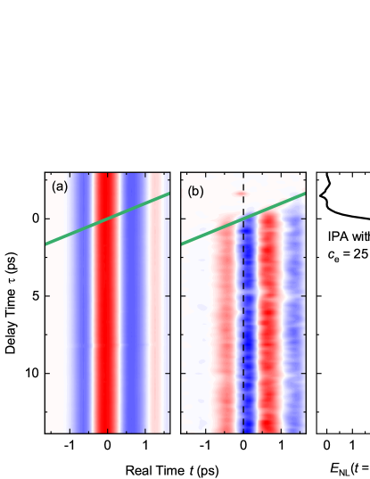
Fig. 1 presents experimental results for an electron concentration of M in IPA. In Fig. 1(a), the THz probe pulse transmitted through the unexcited liquid jet is plotted as a function of real time and delay time . The green line indicates the temporal position of the femtosecond pump pulse, generating electrons via multiphoton ionization. Figure 1(b) shows the nonlinear THz response of the excited sample. The data were filtered applying a 2D Fourier filter with a bandwidth of 4 THz in the 2D spectral domain. rises after excitation at with a step-like character, due to a sudden absorption change within the 0.5 THz bandwidth of the THz probe pulse after electron generation. Figure 1(c) displays a cut along delay time through the maximum of at , which exhibits pronounced oscillations superimposed with the step-like signal. These oscillations arise from coherent polaron oscillations, impulsively excited during the ultrafast relaxation of the photogenerated electrons to a localized ground state.
The polaron consists of an electron which couples via the Coulomb interaction to electronic and nuclear degrees of freedom of the surrounding liquid. The relevant volume of the liquid is roughly set by the (Debye) screening length of Coulomb interaction and can be represented by a sphere of a nanometer diameter [33], containing up to tens of thousands of solvent molecules. The polaron oscillations represent longitudinal modulations of space charge within this volume leading to oscillations of the polaron size, which modify the transverse dielectric function. This mechanism makes the polaron oscillations accessible to optical probing with transverse electric fields. The frequency of the polaron oscillations is set by of the longitudinal macroscopic dielectric function [40], which in the THz frequency range is almost identical to the transverse macroscopic dielectric function [41].
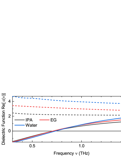
In different polar liquids, the real parts Re( of the macroscopic dielectric functions according to Eq. (1) become very similar for appropriate choices of electron concentrations , as illustrated in Fig. 2 for electron concentrations of , 30 and 40M in IPA, EG and water. All three curves display a zero crossing at about THz and very similar dispersion in the low-frequency THz range.
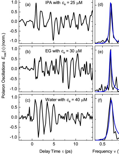
Figure 3(a) shows the polaron oscillations in IPA extracted by subtracting the step-like contribution from the cut in Fig. 1(c). In Figs. 1(b, c), the same procedure was applied to equivalent data sets measured in EG and water. All three transients are normalized to their maximum and show clear oscillations for delay times , which span in the cases of IPA and EG [cf. Figs. 3(a, b)] the whole time range, reflecting the highly underdamped character of the polaron oscillations. The oscillations in water subside on a time scale of about 5 ps due to Debye relaxation of water molecules. In Figs. 3(d-f), the Fourier transforms of the oscillations are plotted as a function of frequency, exhibiting pronounced peaks at about 0.7 THz. The linewidth and center frequency of these peaks is well reproduced by the imaginary part of the reciprocal dielectric function of the neat liquids around (cf. Eq. 8). The spectral widths of the spectra are large compared to a potential linewidth caused by the damping of the electron polarizability (Eq.2). For the current choice of electron concentrations in IPA and EG, relation (12) is approximately fulfilled, resulting in very similar line shapes of the polaron resonances [blue curves in Figs. 3(d) and (e)].
Conclusions and Outlook: The results presented here demonstrate the degree to which polaron response can be controlled both by a femtosecond nonlinear generation of free electron density (setting frequency), and THz probe pulse (controlling amplitude). From this perspective, it is possible for appropriate choices of electron concentration and THz probe frequency to create polar impostorons, where the polaron response of distinct liquids is rendered indistinguishable. The exception to this controllability is the damping, e.g., due to Debye relaxation, which manifests in the imaginary part of the dielectric function of the neat liquids. It is for this reason that in Figs. 3(a-c), the polaron oscillations in water decay on a faster time scale than in the alcohols and, thus, relation (12) cannot be fulfilled for a pair consisting of water and an alcohol. On the other hand, the small imaginary part of the THz dielectric function in alcohols can be made nearly identical in the frequency range between 1.0 and 1.5 THz, as is evident from the linear THz spectra reported in Ref. [42].
Since their inception, “driven imposters” [19] have been considered merely a theoretical curiosity – until now. This work marks a new direction in experimental quantum technology by demonstrating the unique possibilities predicted by quantum tracking control. The present experimental accessibility of polaron dynamics suggests that they are good candidates for the realisation of other exotic optical effects, beyond the creation of driven imposters. In particular, the tracking control formalism has recently been deployed to dynamically generate an epsilon near-zero (ENZ) response [43, 44] in a material [45]. An immediate future extension of the work presented here is therefore to extend it to this scenario, dynamically generating ENZ-like responses in polaronic systems.
Acknowledgments:
T.E. and D.I.B. are grateful to the Alexander von Humboldt Foundation for organizing the 11th Humboldt Award Winners’ Forum, where this collaboration was conceived. D.I.B. was supported by Army Research Office (ARO) (grant W911NF-23-1-0288; program manager Dr. James Joseph), while G.M. is supported by the European Research Council (ERC) under the European Union’s Horizon 2020 Research and Innovation Program (grant agreement 833365). The views and conclusions contained in this document are those of the authors and should not be interpreted as representing the official policies, either expressed or implied, of ARO or the U.S. Government. The U.S. Government is authorized to reproduce and distribute reprints for Government purposes notwithstanding any copyright notation herein. We thank A. Ghalgaoui, J. Zhang, and P. Singh for their contributions to the experimental work. This research has received funding from the European Research Council (ERC) under the European Union’s Horizon 2020 Research and Innovation Program (Grant No. 833365). D.I.B. and D.T. are also supported by by the W. M. Keck Foundation.
G.M. and M.R. contributed equally to this work.
References
- Kieu [2003] T. D. Kieu, Quantum Algorithm for Hilbert’s Tenth Problem, International Journal of Theoretical Physics 42, 1461 (2003).
- Bondar and Pechen [2020] D. I. Bondar and A. N. Pechen, Uncomputability and complexity of quantum control, Scientific Reports 10, 1195 (2020), publisher: Nature Publishing Group.
- Magann et al. [2021] A. B. Magann, C. Arenz, M. D. Grace, T.-S. Ho, R. L. Kosut, J. R. McClean, H. A. Rabitz, and M. Sarovar, From Pulses to Circuits and Back Again: A Quantum Optimal Control Perspective on Variational Quantum Algorithms, PRX Quantum 2, 010101 (2021).
- Magann et al. [2022a] A. B. Magann, K. M. Rudinger, M. D. Grace, and M. Sarovar, Lyapunov-control-inspired strategies for quantum combinatorial optimization, Physical Review A 106, 062414 (2022a).
- McCaul et al. [2023] G. McCaul, K. Jacobs, and D. I. Bondar, Towards single atom computing via high harmonic generation, The European Physical Journal Plus 138, 123 (2023).
- Glaser et al. [2015] S. J. Glaser, U. Boscain, T. Calarco, C. P. Koch, W. Köckenberger, R. Kosloff, I. Kuprov, B. Luy, S. Schirmer, T. Schulte-Herbrüggen, D. Sugny, and F. K. Wilhelm, Training Schrödinger’s cat: quantum optimal control, The European Physical Journal D 69, 279 (2015).
- Koch [2016] C. P. Koch, Controlling open quantum systems: tools, achievements, and limitations, Journal of Physics: Condensed Matter 28, 213001 (2016), publisher: IOP Publishing.
- Zhu and Rabitz [2003] W. Zhu and H. Rabitz, Quantum control design via adaptive tracking, The Journal of Chemical Physics 119, 3619 (2003).
- Gross et al. [1993] P. Gross, H. Singh, H. Rabitz, K. Mease, and G. M. Huang, Inverse quantum-mechanical control: A means for design and a test of intuition, Physical Review A 47, 4593 (1993), publisher: American Physical Society.
- Ong et al. [1984] C. K. Ong, G. M. Huang, T. J. Tarn, and J. W. Clark, Invertibility of quantum-mechanical control systems, Mathematical systems theory 17, 335 (1984).
- Rothman et al. [2005] A. Rothman, T.-S. Ho, and H. Rabitz, Observable-preserving control of quantum dynamics over a family of related systems, Physical Review A 72, 023416 (2005).
- Sahebi and Yarahmadi [2018] Z. Sahebi and M. Yarahmadi, Switching optimal adaptive trajectory tracking control of quantum systems, Optimal Control Applications and Methods 39, 1323 (2018), _eprint: https://onlinelibrary.wiley.com/doi/pdf/10.1002/oca.2412.
- Mirrahimi et al. [2005] M. Mirrahimi, G. Turinici, and P. Rouchon, Reference Trajectory Tracking for Locally Designed Coherent Quantum Controls, The Journal of Physical Chemistry A 109, 2631 (2005).
- Coron et al. [2009] J.-M. Coron, A. Grigoriu, C. Lefter, and G. Turinici, Quantum control design by Lyapunov trajectory tracking for dipole and polarizability coupling, New Journal of Physics 11, 105034 (2009).
- Campos et al. [2017] A. G. Campos, D. I. Bondar, R. Cabrera, and H. A. Rabitz, How to Make Distinct Dynamical Systems Appear Spectrally Identical, Physical Review Letters 118, 083201 (2017), publisher: American Physical Society.
- Magann et al. [2018] A. Magann, T.-S. Ho, and H. Rabitz, Singularity-free quantum tracking control of molecular rotor orientation, Physical Review A 98, 043429 (2018).
- Magann et al. [2023] A. B. Magann, T.-S. Ho, C. Arenz, and H. A. Rabitz, Quantum tracking control of the orientation of symmetric-top molecules, Physical Review A 108, 033106 (2023).
- Chen et al. [1995] Y. Chen, P. Gross, V. Ramakrishna, H. Rabitz, and K. Mease, Competitive tracking of molecular objectives described by quantum mechanics, The Journal of Chemical Physics 102, 8001 (1995).
- McCaul et al. [2020a] G. McCaul, C. Orthodoxou, K. Jacobs, G. H. Booth, and D. I. Bondar, Driven Imposters: Controlling Expectations in Many-Body Systems, Physical Review Letters 124, 183201 (2020a).
- McCaul et al. [2020b] G. McCaul, C. Orthodoxou, K. Jacobs, G. H. Booth, and D. I. Bondar, Controlling arbitrary observables in correlated many-body systems, Physical Review A 101, 053408 (2020b).
- Magann et al. [2022b] A. B. Magann, G. McCaul, H. A. Rabitz, and D. I. Bondar, Sequential optical response suppression for chemical mixture characterization, Quantum 6, 626 (2022b), publisher: Verein zur Förderung des Open Access Publizierens in den Quantenwissenschaften.
- McCaul et al. [2021] G. McCaul, A. F. King, and D. I. Bondar, Optical Indistinguishability via Twinning Fields, Physical Review Letters 127, 113201 (2021).
- McCaul et al. [2022] G. McCaul, A. F. King, and D. I. Bondar, Non‐Uniqueness of Driving Fields Generating Non‐Linear Optical Response, Annalen der Physik 534, 2100523 (2022).
- Zhang et al. [2005] Zhang, A. S. Keys, T. Chen, and S. C. Glotzer, Self-assembly of patchy particles into diamond structures through molecular mimicry, Langmuir 21, 11547 (2005).
- Whitesell et al. [1994] J. K. Whitesell, R. E. Davis, M. S. Wong, and N. L. Chang, Molecular crystal engineering by shape mimicry, J. Am. Chem. Soc. 116, 523 (1994).
- Gust et al. [1993] D. Gust, T. A. Moore, and A. L. Moore, Molecular mimicry of photosynthetic energy and electron transfer, Accs. Chem. Res. 26, 198 (1993).
- Rabong et al. [2014] C. Rabong, C. Schuster, T. Liptaj, N. Pronayova, V. B. Delchev, U. Jordis, and J. Phopase, Nxo beta structure mimicry: an ultrashort turn/hairpin mimic that folds in water, RSC Adv. 4, 21351 (2014).
- Della Gaspera et al. [2014] E. Della Gaspera, J. van Embden, A. S. R. Chesman, N. W. Duffy, and J. J. Jasieniak, Mimicry of sputtered i-zno thin films using chemical bath deposition for solution-processed solar cells, ACS Appl. Mater. Interfaces 6, 22519 (2014).
- Marsalek et al. [2012] O. Marsalek, F. Uhlig, J. VandeVondele, and P. Jungwirth, Structure, Dynamics, and Reactivity of Hydrated Electrons by Ab Initio Molecular Dynamics, Accounts of Chemical Research 45, 23 (2012), publisher: American Chemical Society.
- Turi and Rossky [2012] L. Turi and P. J. Rossky, Theoretical Studies of Spectroscopy and Dynamics of Hydrated Electrons, Chemical Reviews 112, 5641 (2012), publisher: American Chemical Society.
- Herbert [2019] J. M. Herbert, Structure of the aqueous electron, Physical Chemistry Chemical Physics 21, 20538 (2019).
- Ghalgaoui et al. [2021] A. Ghalgaoui, B. P. Fingerhut, K. Reimann, T. Elsaesser, and M. Woerner, Terahertz polaron oscillations of electrons solvated in liquid water, Phys. Rev. Lett. 126, 097401 (2021).
- Singh et al. [2022] P. Singh, J. Zhang, A. Ghalgaoui, K. Reimann, B. P. Fingerhut, M. Woerner, and T. Elsaesser, Coherent polaron dynamics of electrons solvated in polar liquids, PNAS Nexus 1, pgac078 (2022).
- Runge et al. [2023] M. Runge, K. Reimann, M. Woerner, and T. Elsaesser, Nonlinear terahertz polarizability of electrons solvated in a polar liquid, Phys. Rev. Lett. 131, 166902 (2023).
- Gaal et al. [2007] P. Gaal, W. Kuehn, K. Reimann, M. Woerner, T. Elsaesser, and R. Hey, Internal motions of a quasiparticle governing its ultrafast nonlinear response, Nature 450, 1210 (2007), publisher: Nature Publishing Group.
- Lee et al. [1953] T. D. Lee, F. E. Low, and D. Pines, The Motion of Slow Electrons in a Polar Crystal, Physical Review 90, 297 (1953), publisher: American Physical Society.
- Fröhlich [1954] H. Fröhlich, Electrons in lattice fields, Advances in Physics 3, 325 (1954), publisher: Taylor & Francis _eprint: https://doi.org/10.1080/00018735400101213.
- Hannay [1983] J. H. Hannay, The Clausius-Mossotti equation: an alternative derivation, Eur. J. Phys. 4, 141 (1983).
- Kubo [1957] R. Kubo, Statistical-Mechanical Theory of Irreversible Processes. I. General Theory and Simple Applications to Magnetic and Conduction Problems, J. Phys. Soc. Jpn. 12, 570 (1957).
- Fuchs and Kliewer [1968] R. Fuchs and K. L. Kliewer, Optical modes of vibration in an ionic crystal sphere, J. Opt. Soc. Am. 58, 319 (1968).
- Bopp et al. [1998] P. A. Bopp, A. A. Kornyshev, and G. Sutmann, Frequency and wave-vector dependent dielectric function of water: Collective modes and relaxation spectra, J. Chem. Phys. 109, 1939 (1998).
- Mazaheri et al. [2024] Z. Mazaheri, G. P. Papari, and A. Andreone, Dielectric response of different alcohols in water-rich binary mixtures from THz ellipsometry, Int. J. Mol. Sci. 25, 4240 (2024).
- Wu et al. [2021] J. Wu, Z. T. Xie, Y. Sha, H. Y. Fu, and Q. Li, Epsilon-near-zero photonics: infinite potentials, Photon. Res. 9, 1616 (2021).
- Niu et al. [2018] X. Niu, X. Hu, S. Chu, and Q. Gong, Epsilon-near-zero photonics: A new platform for integrated devices, Advanced Optical Materials 6, 1701292 (2018), https://onlinelibrary.wiley.com/doi/pdf/10.1002/adom.201701292 .
- Masur et al. [2023] J. Masur, D. I. Bondar, and G. McCaul, Dynamical generation of epsilon-near-zero behaviour via tracking and feedback control (2023), arXiv:2301.12069 .