Full Stokes-vector inversion of the solar Mg II h & k lines

Abstract

The polarization of the Mg II h & k resonance lines is the result of the joint action of scattering processes and the magnetic field induced Hanle, Zeeman, and magneto-optical effects, thus holding significant potential for the diagnostic of the magnetic field in the solar chromosphere. The Chromospheric LAyer Spectro-Polarimeter sounding rocket experiment, carried out in 2019, successfully measured at each position along the 196 arcsec spectrograph slit the wavelength variation of the four Stokes parameters in the spectral region of this doublet around $280$ nm, both in an active region plage and in a quiet region close to the limb. We consider some of these CLASP2 Stokes profiles and apply to them the recently-developed HanleRT Tenerife Inversion Code, which assumes a one-dimensional model atmosphere for each spatial pixel under consideration (i.e., it neglects the effects of horizontal radiative transfer). We find that the non-magnetic causes of symmetry breaking, due to the horizontal inhomogeneities and the gradients of the horizontal components of the macroscopic velocity in the solar atmosphere, have a significant impact on the linear polarization profiles. By introducing such non-magnetic causes of symmetry breaking as parameters in our inversion code, we can successfully fit the Stokes profiles and provide an estimation of the magnetic field vector. For example, in the quiet region pixels, where no circular polarization signal is detected, we find that the magnetic field strength in the upper chromosphere varies between 1 and 20 gauss.

1 Introduction

The magnetic field permeating the solar atmosphere plays a key role in its structure, energy transfer, and the eventual eruptive phenomena. The inference of the magnetic field in the photosphere usually relies on the use of inversion codes of polarization signals magnetically induced by the Zeeman effect (del Toro Iniesta & Ruiz Cobo, 2016; Lagg et al., 2017; de la Cruz Rodríguez & van Noort, 2017). The amplitude of the circular polarization caused by the Zeeman effect scales with the ratio (generally smaller than unity) between the Zeeman splitting and the Doppler line width, while the linear polarization signals scale with the square of this quantity (Landi Degl’Innocenti & Landolfi, 2004). Chromospheric lines tend to be wider than photospheric lines, and the magnetic field generally decreases with height. For these reasons, the inference of chromospheric magnetic fields via the Zeeman effect becomes considerably more challenging, except in active regions where its circular polarization signals can be measured even in strong ultraviolet lines like Mg II h & k (Ishikawa et al., 2021; Li et al., 2023).

The Hanle effect is the magnetically induced modification of the linear polarization caused by the scattering of anisotropic radiation in a spectral line and holds significant potential for the diagnostic of magnetic fields, albeit being significantly more difficult to exploit (e.g., the monograph by Landi Degl’Innocenti & Landolfi, 2004). Motivated by the theoretical investigations on the polarization caused by scattering processes and the Hanle and Zeeman effects in the Mg II h & k lines around 280 nm (Belluzzi & Trujillo Bueno 2012; Alsina Ballester et al. 2016; del Pino Alemán et al. 2016, and del Pino Alemán et al. 2020) the Chromospheric LAyer SpectroPolarimeter (CLASP2; Narukage et al. 2016; Song et al. 2018) suborbital rocket experiment was carried in 2019 with the aim of observing the four Stokes parameters in this ultraviolet spectral region and inferring the magnetic field vector in the chromosphere. The mission was successful and obtained unprecedented spectropolarimetric data of this spectral region in both a quiet region close to the solar limb (Rachmeler et al., 2022) and in an active region plage (Ishikawa et al., 2021). The CLASP2 spectropolarimetric observations confirmed the theoretical predictions based on the quantum theory of spectral line polarization (see the review by Trujillo Bueno & del Pino Alemán, 2022), which showed that the combined action of partial frequency redistribution (PRD) effects and quantum mechanical interference between the magnetic sublevels pertaining to the two upper $J$-levels of the Mg II h & k lines (hereafter, $J$-state interference) produce sizable scattering polarization signals in the near and far wings of these lines (Belluzzi & Trujillo Bueno, 2012), and that such signals are sensitive to the magnetic field via the magneto-optical (MO) terms of the Stokes-vector transfer equation (Alsina Ballester et al., 2016; del Pino Alemán et al., 2016).

While there are well-known Stokes inversion codes like HAZEL (Asensio Ramos et al., 2008) which exploit scattering polarization and the Hanle and Zeeman effects assuming complete frequency redistribution (CRD) and a constant-property slab of plasma levitating at a given height above the solar visible disk, until very recently there was no inversion code capable of tackling the inversion of Stokes profiles caused by the joint action of all the above-mentioned effects in strong chromospheric lines, like those of the Mg II h & k doublet. These resonance lines show both significant PRD and radiation transfer (RT) effects, and their forward modeling requires solving the problem of the generation and transfer of polarized radiation out of thermodynamic equilibrium (non-LTE) accounting for PRD, scattering polarization, $J$-state interference, and the Hanle, Zeeman, and MO effects in the general magnetic field regime (incomplete Paschen-Back regime) in an optically thick plasma. In order to tackle this inversion problem, we recently developed the Stokes HanleRT Tenerife Inversion code (HanleRT-TIC) (Li et al., 2022), based on the HanleRT forward solver (del Pino Alemán et al., 2016, 2020).

The intensity and circular polarization profiles observed by CLASP2 in an active region plage have been exploited by applying the weak field approximation (Ishikawa et al., 2021; Afonso Delgado et al., 2023) and the HanleRT-TIC inversion code (Li et al., 2023), obtaining an unprecedented map of the longitudinal component of the magnetic field from the photosphere to the upper chromosphere, just below the transition region. The linear polarization observed by CLASP2 across the Mg II h & k lines was shown in Rachmeler et al. (2022), comparing the CLASP2 observations of the quiet Sun target with the theoretical predictions of Belluzzi & Trujillo Bueno (2012) in an unmagnetized semi-empirical model of the quiet solar atmosphere; the authors argued that horizontal inhomogeneities and magnetic fields are needed to explain the observed signals and their spatial variations.

In a one-dimensional (1D) model atmosphere, static or without horizontal components of the plasma macroscopic velocity, the only way to break the axial symmetry of the radiation field that illuminates each spatial point within the medium is by the presence of a magnetic field inclined with respect to the vertical axis, the axis along which the model’s physical quantities vary. However, at each height in the real solar atmosphere we have horizontal inhomogeneities in the plasma temperature and density, as well as macroscopic motions with spatial gradients also in the horizontal component of the velocity. Therefore, in general, in the real solar atmosphere the radiation field does not have axial symmetry around the solar radius vector through the spatial point under consideration, even in the absence of a magnetic field (e.g., Jaume Bestard et al., 2021). The impact of such non-magnetic causes of symmetry breaking on the linear polarization caused by the scattering of anisotropic radiation in the Mg II h & k lines can be modeled applying a three-dimensional (3D) RT code, but the development of such a code with PRD and $J$-state interference capable of performing calculations in realistic 3D models with today’s supercomputer facilities is still an unachieved challenge. Our HanleRT-TIC takes into account the effects of PRD and $J$-state interference in the presence of arbitrary magnetic fields, but ignoring the effects of horizontal radiative transfer (i.e., HanleRT-TIC is a 1D plane-parallel RT code for the synthesis and inversion of Stokes profiles). The only way of bypassing this issue in 1D geometry, i.e., without solving the full 3D RT problem, is by parameterizing this missing contribution to the lack of axial symmetry. HanleRT-TIC allows such a functionality.

Our first step in this work is to estimate the magnetic field vector in the chromosphere through the application of the HanleRT-TIC to some of the Stokes profiles of the Mg II h & k lines observed by CLASP2. To this end, after briefly describing in Section 2 the CLASP2 observations, in Section 3 we describe our parameterized approach to account for the impact of the above-mentioned non-magnetic causes of symmetry breaking in our pixel by pixel inversions with HanleRT-TIC. The inversion of four representative Mg II h & k Stokes profiles are shown in Section 4. Section 5 discusses possible degeneracies introduced by our parameterization of the non-magnetic causes of symmetry breaking and how they affect the inferred magnetic field. Finally, Section 6 summarizes our main conclusions.

2 Summary of the CLASP2 observations

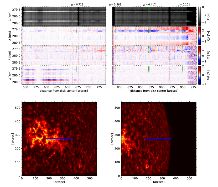
Figure 1: In the top panels, intensity (in log-scale and normalized to the maximum) and Stokes fractional polarization ($Q/I$, $U/I$, and $V/I$) profiles obtained by the CLASP2. In the bottom panels, slit-jaw images in the H I Lyman-$\alpha$ line recorded by CLASP2. The left and right columns correspond to the observations of the plage and limb targets, respectively. The regions delimited by green dashed lines in the top panels indicate the locations of the 4 spatially averaged profiles in Figs. 2–5. The blue lines in the bottom panels indicate the position of the spectrograph’s slit.

The data used in this work were obtained by the CLASP2 suborbital space mission on 11 April 2019. Sit-and-stare observations were carried out with the 196 arcsec spectrograph slit located at three consecutive positions on the solar disk, namely the disk center, an active region plage at the east side of NOAA 12738 with a nearby enhanced network, and a quiet Sun region near the north-east limb. The plage and quiet-Sun target observations were obtained between 16:53:40 and 16:56:16 UT (156 s) and between 16:56:25 and 16:58:45 UT (140 s), respectively (Ishikawa et al., 2021). The temporally averaged signals have a polarization accuracy better than 0.1% (Song et al., 2022).

The spectral range of CLASP2 is between 279.30 and 280.68 nm, with a sampling of 49.9 mÅ/pixel. The spectral point spread function can be approximated with a gaussian with a full width at half maximum (FWHM) of 110 mÅ (Song et al., 2018; Tsuzuki et al., 2020). The CLASP2 spectral range contains the Mg II h and k lines at 279.6 and 280.3 nm, respectively, two Mg II blended transitions at 279.88 nm, whose lower level are the upper levels of the h & k lines, as well as several other lines (e.g., the Mn I resonance lines at 279.91 and 280.19 nm).

The temporally averaged observations of the plage and quiet-Sun limb targets are shown in Fig. 1. The circular polarization caused by the Zeeman effect is clearly prominent in about 2/3 of the plage target (between 540 and 670 arcsec), faint in the nearby enhanced network (between 670 and 740 arcsec), and non-detected in the quiet region closer to the limb (right panels in Fig. 1). The linear polarization follows almost the opposite behavior, with weaker scattering polarization signals within the plage region due to the Hanle and MO depolarization caused by its stronger magnetic fields. Although in the quiet region the circular polarization was not detected, the estimation of the magnetic field vector is still possible via the Hanle effect in the Mg ii k line. Given the significant computational demand of full Stokes inversions with scattering polarization and the novelty of the inversion approach in this work, here we focus on four representative profiles located at heliocentric angles, $\theta$, with $\mu=\cos{\theta}=0.712$, 0.563, 0.417, and 0.101. At each of these locations, we have spatially averaged the observed Stokes profiles at a few adjacent pixels (3, 2, 3, and 7 pixels, respectively) sharing similar profiles, increasing the signal to noise ratio without causing significant cancellations of the observed polarization signals. We show as example the Stokes profiles for the individual pixels included in the average at $\mu=0.712$ in Appendix A.

3 The Stokes inversion strategy

In this section we describe the inversion strategy we have applied to infer the magnetic field vector from the observed Stokes profiles, showing illustrative results for a point on the plage target and at three locations on the quiet Sun target. In particular, we explain the parameterization we have included in the HanleRT-TIC in order to account for the possible impact of the non-magnetic causes of symmetry breaking due to the presence of horizontal inhomogeneities and macroscopic horizontal motions.

3.1 Parameterization of the axial symmetry breaking

At each iterative step needed for solving the non-LTE Stokes inversion problem the HanleRT-TIC solves the non-LTE spectral synthesis problem of the generation and transfer of polarized radiation assuming 1D plane-parallel geometry. Therefore, at each pixel the inversion of the emergent Stokes profiles is done assuming that there is no radiative interaction with the surrounding pixels. In other words, the effects of horizontal RT in the solar atmosphere (because it is a 3D plasma) are neglected. With such an approximation in HanleRT-TIC any breaking of the axial symmetry of the pumping radiation field would be due to a non-vertical magnetic field vector and/or to vertical gradients in the horizontal components of the macroscopic velocity, because at each height in a 1D plane-parallel model all the quantities are assumed to be the same along the horizontal directions. However, in the solar atmosphere, or in a three-dimensional (3D) model atmosphere, the horizontal RT effects resulting from the horizontal inhomogeneities in the physical properties of the plasma break the axial symmetry of the radiation field that illuminates each spatial point within the medium. Such non-magnetic causes of symmetry breaking are important, because they can have a significant impact on the linear polarization caused by the scattering of anisotropic radiation in a spectral line (e.g., Manso Sainz & Trujillo Bueno, 2011; del Pino Alemán et al., 2018; Jaume Bestard et al., 2021).

The degree of axial symmetry breaking in the radiation field illuminating each spatial point within a model atmosphere is quantified by the $Q\neq 0$ components of the $J^{K}_{Q}$ radiation field tensor (for a detailed derivation and description of these tensors, see Landi Degl’Innocenti & Landolfi, 2004). As explained above, when solving the spectral synthesis problem pixel by pixel assuming 1D plane-parallel geometry we miss contributions to these components of the radiation field tensor that can be important for the linear polarization. What we propose in this work is to parameterize the missing contributions as ad-hoc contributions to the radiation field tensors in HanleRT-TIC, by defining a new set of $J^{\prime K}_{Q}$ tensor components as

$$J^{\prime 2}_{1} =J^{2}_{1}+{J^{\dagger}}^{2}_{1},$$ (1a)

$$J^{\prime 2}_{2} =J^{2}_{2}+{J^{\dagger}}^{2}_{2},$$ (1b)

where $J^{2}_{1}$ and $J^{2}_{2}$ are the tensor components calculated by integrating the Stokes parameters (see Landi Degl’Innocenti & Landolfi, 2004) resulting from the solution of the RT equations, $J^{\prime 2}_{1}$ and $J^{\prime 2}_{2}$ are the final values that go into the statistical equilibrium equations (SEE) and the emissivity in the RT equations, and ${J^{\dagger}}^{2}_{1}$ and ${J^{\dagger}}^{2}_{2}$ are the ad-hoc parameterized additional contributions. We do not consider ad-hoc contributions to the $J^{1}_{1}$ component because it does not impact the emergent linear polarization profiles. The ad-hoc components of the radiation field tensor are then

$${J^{\dagger}}^{2}_{1} =r_{1}J^{0}_{0}+i_{1}J^{0}_{0}i,$$ (2a)

$${J^{\dagger}}^{2}_{2} =r_{2}J^{0}_{0}+i_{2}J^{0}_{0}i,,$$ (2b)

where $i$ is the imaginary unit and $J^{0}_{0}$ is the component of the radiation field tensor corresponding to the mean intensity, calculated by integrating the Stokes $I$ parameter resulting from the solution of the RT equations (see Landi Degl’Innocenti & Landolfi, 2004). The coefficients $r_{1}$, $i_{1}$, $r_{2}$, and $i_{2}$ are parameters in the inversion. The relation between these quantities and the Stokes parameters for the linear polarization has been previously exploited by Zeuner et al. (2020, 2024) in their observational study of the scattering polarization in the Sr I photospheric line at 4607 Å. Hereafter, we use $J^{\dagger}$ to refer to the set of four ad-hoc contributions of the radiation field tensor, $r_{1}$, $i_{1}$, $r_{2}$, and $i_{2}$, which we quantify below in percentage of the $J^{0}_{0}$ component.

3.2 Inversion cycles and nodes

We have applied an inversion strategy similar to that outlined in Li et al. (2023), with two cycles to invert the temperature ($T$), the bulk vertical velocity ($v_{z}$), the micro-turbulent velocity ($v_{\rm turb}$), and the gas pressure at the top boundary ($P_{\rm g}$) from the Stokes $I$ profile (hereafter, the non-magnetic cycles). The first cycle has four nodes in $T$ and three in $v_{z}$ and $v_{\rm turb}$, while the second one has seven and four, respectively. In these non-magnetic cycles the velocity is assumed to be parallel to the local vertical because it significantly decreases the computational demands. Once the Stokes $I$ profiles are fitted, $T$, $v_{z}$, $v_{\rm turb}$, and $P_{\rm g}$ are fixed.

In the subsequent cycles we retrieve the magnetic field and $J^{\dagger}$ from Stokes $Q$, $U$, and $V$ (hereafter, the magnetic cycles). The Stokes inversion gives us the longitudinal component of the magnetic field ($B_{\parallel}$), the transverse component of the magnetic field with respect to the line of sight (LOS; $B_{\perp}$), and the azimuth of the magnetic field vector in the plane perpendicular to the LOS ($\phi_{B_{\perp}}$). We use these components of the magnetic field vector because Stokes $U$ in the wings of the Mg II h & k lines is sensitive to the sign of $B_{\parallel}$ through the MO effects, although the addition of $J^{\dagger}$ can alter this dependency. We also provide the magnetic field strength ($B$), the magnetic field inclination ($\theta_{B}$) with respect to the local vertical, and the azimuth of the magnetic field ($\chi_{B}$) in the local reference frame because it can be helpful to study the Hanle effect ambiguities. The details of the number of cycles and nodes are different for each of the four selected Stokes profiles, and they are described in Sec. 4.

In all inversion cycles the spectral syntheses are performed in a model atmosphere with 60 non-equally spaced layers between ${\rm log_{10}}(\tau_{500})=-8.0$ and $1.0$. The errors are computed from the diagonal of the Hessian matrix (see Li et al., 2022).

4 Results

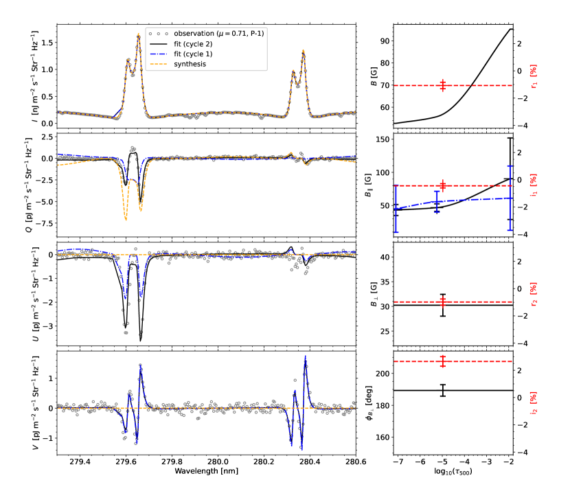
Figure 2: Left column: from top to bottom, Stokes $I$, $Q$, $U$, and $V$ profiles, respectively. The open circles correspond to the temporally and spatially averaged observed Stokes profiles. The dash-dotted blue and solid black curves are the inversion fit from the first and the second magnetic cycles, respectively, while the dashed orange curves show the profile synthesized in the inverted atmosphere neglecting the magnetic field. Note that the $k_{\rm 1v}$ minimum at around 279.57 nm is blended with a Mn I resonance line and that the corresponding wavelength points are not considered in the inversion, resulting in a straight line in the fit. Right column: from top to bottom, magnetic field strength, magnetic field longitudinal component, magnetic field transversal component, and magnetic field azimuth in the plane perpendicular to the LOS, in solid black (dash-dotted blue) curves from the second (first) magnetic cycle (left axis), respectively, and the real part of the $Q=1$ tensor, the imaginary part of the $Q=1$ tensor, the real part of the $Q=2$ tensor, and the imaginary part of the $Q=2$ tensor characterizing the lack of axial symmetry, in dashed red curves (right axis), respectively. This case corresponds to P-1, a region at the edge of the plage ($\mu=0.712$ in Fig. 1).

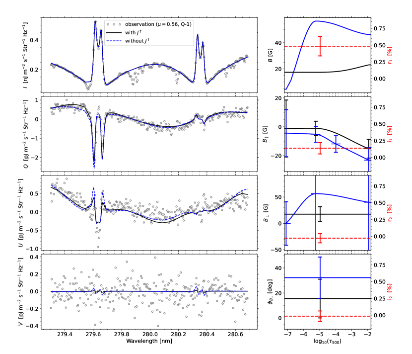
Figure 3: Left column: from top to bottom, Stokes $I$, $Q$, $U$, and $V$ profiles, respectively. The open circles correspond to the temporally and spatially averaged observed Stokes profiles. The solid black (blue) curves are the inversion fit when accounting for (neglecting) the parameters for the horizontal inhomogeneity. Right column: from top to bottom, magnetic field strength, magnetic field longitudinal component, magnetic field transversal component, and magnetic field azimuth in the plane perpendicular to the LOS, in solid black (blue) curves for the inversion accounting for (neglecting) the parameters for the horizontal inhomogeneity (left axis), respectively, and the real part of the $Q=1$ tensor, the imaginary part of the $Q=1$ tensor, the real part of the $Q=2$ tensor, and the imaginary part of the $Q=2$ tensor characterizing the lack of axial symmetry, in dashed red curves (right axis), respectively. This case corresponds to Q-1, a region in the quiet Sun ($\mu=0.563$ in Fig. 1).

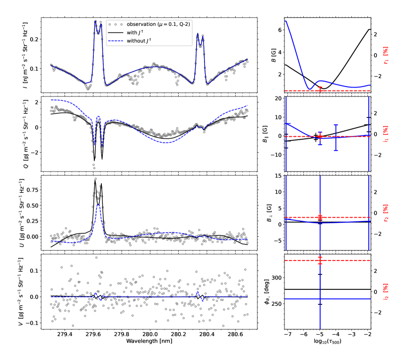
Figure 4: Same as Fig. 3, but for Q-2, the region in the quiet Sun with $\mu=0.101$ (see Fig. 1).

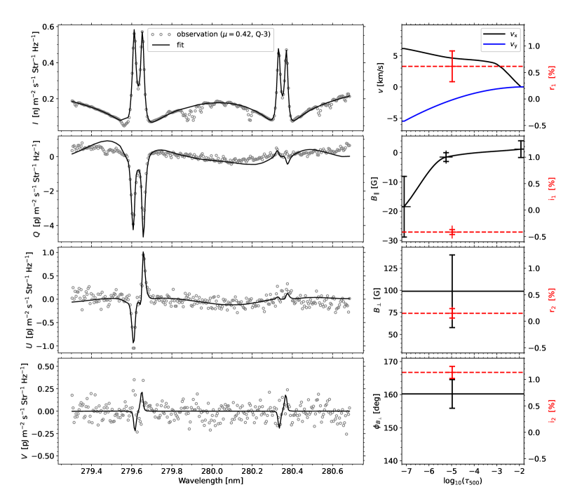
Figure 5: Left column: from top to bottom, Stokes $I$, $Q$, $U$, and $V$ profiles, respectively. The open circles correspond to the temporally and spatially averaged observed Stokes profiles. The solid black curves are the inversion fit. Right column: from top to bottom, horizontal component of the plasma velocity, magnetic field longitudinal component, magnetic field transversal component, and magnetic field azimuth in the plane perpendicular to the LOS, in solid black curves (left axis), respectively, and the real part of the $Q=1$ tensor, the imaginary part of the $Q=1$ tensor, the real part of the $Q=2$ tensor, and the imaginary part of the $Q=2$ tensor characterizing the lack of axial symmetry, in dashed red curves (right axis), respectively. The black solid curve in the velocity panel corresponds to the component in the plane containing the LOS and the local vertical (x component), while the blue solid curve corresponds to the component perpendicular to the same plane (y component). This case corresponds to Q-3, a region in the quiet Sun ($\mu=0.417$ in Fig. 1).

In this section we show the results of applying the HanleRT-TIC to invert the Stokes profiles observed by CLASP2 at four representative locations, one just at the edge of the plage target (where the circular polarization caused by the Zeeman effect was detected, hereafter P-1) and three positions in the quiet-Sun target (where the measured circular polarization was at the noise level). In all cases, the Stokes $Q$ and $U$ profiles were detected, which result from the combined action of scattering processes and the Hanle and MO effects. As shown below, in one of the chosen locations the Stokes profiles could be fitted without introducing $J^{\dagger}$ (hereafter Q-1), while in another location the Stokes profiles could only be fitted with $J^{\dagger}$ (i.e., by acknowledging a non-magnetic cause of axial symmetry breaking, hereafter Q-2). Interestingly, the Stokes profiles of one of the chosen locations could only be fitted via the axial symmetry breaking that results from a vertical gradient in the horizontal component of the macroscopic velocity (hereafter Q-3).

4.1 Stokes profiles at the edge of the plage (P-1)

The open circles of Fig. 2 show the CLASP2 Stokes profiles at the edge of the plage target (see the $\mu=0.712$ location in Fig. 1), where we have significant linear and circular polarization signals. The orange dashed curves in Fig. 2 show the Stokes profiles calculated in the model atmosphere that results from the first two cycles of the inversion (i.e., without magnetic field or $J^{\dagger}$). As expected, due to the axial symmetry of the model and the absence of magnetic field, Stokes $U$ and $V$ are zero. Notably, the right trough of the k line in the synthetic Stokes $Q$ profile shows a similar amplitude to the observation. Typically, the impact of the Hanle and/or MO effects is to depolarize and rotate the linear polarization ($Q\rightarrow U$ in this case). It is thus impossible to find a magnetic field vector such that all Stokes $Q$, $U$, and $V$ profiles are fitted at the same time. The addition of the $J^{\dagger}$ contribution is necessary to achieve a good fit. This is not surprising, because at the edge of the plage we can expect a significant lack of axial symmetry, as seen in Fig. 2 of Ishikawa et al. (2023).

We invert the polarization profiles in two magnetic cycles. In the first cycle we retrieve the longitudinal component of the magnetic field with 3 nodes from only Stokes $V$. In this step we assumme that the magnetic field is vertical so the problem is still axially symmetric, allowing for the determination of a better initial guess of the magnetic field without too heavy computational requirements. In the second cycle we infer $B_{\parallel}$ with three nodes, and $B_{\perp}$, $\phi_{B_{\perp}}$, $r_{1}$, $i_{1}$, $r_{2}$, and $i_{2}$ with one node. Although a constant value for these quantities is not realistic, if we manage to fit the observed Stokes profiles it means that there is not enough information to recover their gradient, and it is preferable to keep the compatible model with the minimum degrees of freedom. Moreover, a small number of degrees of freedom results in a lower computational demand and, generally, it helps to avoid local minima in the inversion procedure.

The black curves in the left column of Fig. 2 show the best fit from the full inversion. The magnetic field strength and the LOS components of the magnetic field vector, as well as the value of $J^{\dagger}$, are shown in the right column of the figure. The magnetic field strength decreases from about 60 G at ${\rm log_{10}}(\tau_{500})=-4.0$ to about 55 G at ${\rm log_{10}}(\tau_{500})=-7.0$. The $J^{\dagger}$ values lie between half of a percent and a few percent. The blue curves show the inversion results after the first magnetic cycle, which fits only Stokes $V$. Although the inferred $B_{\parallel}$ values are somewhat different from those from the full Stokes inversion, the values are compatible within the error bars and the Stokes $V$ fits are of similar quality. Since $B_{\parallel}$ also impacts the linear polarization via the MO effect, the full Stokes inversion can better constrain $B_{\parallel}$.

4.2 Quiet Sun Stokes profiles (Q-1)

Figure 3 shows the Stokes profiles of the Mg II h & k lines observed by CLASP2 in the quiet Sun target at $\mu=0.563$ (see Fig. 1). The circular polarization caused by the Zeeman effect is at the noise level, but the linear polarization due to scattering processes is significant, especially in the line wings.

We applied two magnetic cycles to invert these Stokes profiles. In contrast with the plage target profiles studied in Sec. 4.1 (P-1), the circular polarization is now at the noise level, reason why we cannot obtain a first estimation of $B_{\parallel}$ from Stokes $V$. Instead, in the first magnetic cycle we invert the Stokes $Q$, $U$, and $V$ parameters to infer $B_{\parallel}$ with three nodes and $B_{\perp}$ and $\phi_{B_{\perp}}$ with one node. We point out that the linear polarization in the wings of the Mg II h & k lines is sensitive to $B_{\parallel}$, and it is thus necessary to sucessfully fit the observation. Including the Stokes $V$ profile in the inversion, even if the observation shows that the signal is below the noise level, adds a good constraint to the upper value of $B_{\parallel}$. For the initialization we used $B_{\parallel}=0$, $B_{\perp}=10$ G and $\phi_{B_{\perp}}=2.5$ rad (i.e., about $143^{\circ}$). The initial value of $B_{\perp}$ is chosen because the Hanle effect at the center of the k line is sensitive to magnetic fields with strengths between approximately 5 and 100 G, so we initialize the magnetic field in the region of sensitivity. Afterwards, we perform inversions with two extra different cycles. The blue dashed curves in Fig. 3 show the result of an inversion with four nodes for $B_{\parallel}$, and three nodes for $B_{\perp}$ and $\phi_{B_{\perp}}$. The black solid curves in Fig. 3 show the result of an inversion keeping the same number of nodes in $B_{\parallel}$, $B_{\perp}$, and $\phi_{B_{\perp}}$, but adding one node for $r_{1}$, $i_{1}$, $r_{2}$, and $i_{2}$.

As can be seen by comparing the black and blue curves of Fig. 3, the CLASP2 Stokes profiles at the $\mu=0.563$ quiet-Sun target location can be successfully fitted with or without the $J^{\dagger}$ contribution. Although there are evident differences at the plot level, the values of the cost function are similar in both inversions. When the $J^{\dagger}$ contribution is not used in the Stokes inversion, the inferred model shows a steep stratification in $B_{\perp}$ with quite large errors. The inversion with $J^{\dagger}$ gives instead a smoother stratification of $B_{\perp}$ with smaller error bars. The $J^{\dagger}$ values are less than one percent, and the $r_{2}$ and $i_{2}$ components are very close to zero, indicating a relatively weak potential contribution from 3D effects. In any case, both solutions are compatible within the error bars for the noise of the CLASP2 observation, so the differences between the two Stokes inversions we have just described is likely representative of the degree of uncertainty.

4.3 Quiet Sun Stokes profiles (Q-2)

Figure 4 shows the Stokes profiles observed by CLASP2 in the quiet Sun target at $\mu=0.10$. We have performed two inversions with the same nodes and cycles as described above for the Stokes profiles in Fig. 3. In this case, neglecting the contribution of $J^{\dagger}$ cannot provide a good fit to the observed Stokes profiles. The wings of Stokes $Q$ and $U$ are sensitive to the presence of magnetic fields via the MO effects. Because the observed Stokes $U$ at this quiet-Sun location is negligible in the far wings, the inversion without $J^{\dagger}$ predicts $B_{\parallel}=0$ in the upper photosphere, where the far wings originate. However, this constraint is incompatible with the far wings of the observed Stokes $Q$, which cannot be fitted simultaneously (it would be necessary to add $B_{\parallel}$, which in turn would produce a miss-fit in the Stokes $U$ far wings). In addition, this inversion is not able to even reproduce the shape of the Mg II k line in Stokes $U$. It is thus clear that it is necessary to include $J^{\dagger}$ in order to be able to fit the Stokes profiles observed at this quiet-Sun location.

The $J^{\dagger}$ values shown in Fig. 4, of several percent, indicate a significant symmetry breaking contribution from 3D effects. In this inversion the inferred magnetic field is rather weak, of the order of few gauss. Even relatively weak magnetic fields can leave observable imprints in the linear polarization of the Mg II h & k lines. Note, however, that the lower limit to this sensitivity is around 2 gauss, which is approximately one tenth of the critical Hanle field for the Mg II k line.

4.4 Quiet Sun Stokes profiles (Q-3)

At some slit locations in the quiet Sun target, the CLASP2 observations showed antisymmetric Stokes $U$ profiles around the center of the k line. Fig. 5 shows an example, corresponding to a line of sight with $\mu=0.417$, where the Stokes $U$ antisymmetric signal is very significant. This antisymmetric signal cannot be due to cross-talk between the Stokes parameters, not only because the instrumental polarization of CLASP2 is negligible (Song et al., 2022), but also because the observed circular polarization is at the noise level. Based on forward modeling calculations, we have found that neither the magnetic field nor the $J^{\dagger}$ symmetry breaking contributions seem to be able to produce such antisymmetric shapes in the Stokes $U$ profile of the Mg II k line. The only way we have found to fit these profiles (under our assumption of 1D plane-parallel model atmosphere) is via a stratification in the horizontal component of the bulk velocity.

In our inversion of such Stokes profiles we fixed the longitudinal component of the macroscopic velocity from the inversion of Stokes $I$. We then performed another inversion cycle to get the magnetic field vector and $J^{\dagger}$, as well as the velocity component perpendicular to the LOS ($v_{\perp}$) and its azimuth in the plane perpendicular to the LOS ($\phi_{v_{\perp}}$). We inferred $B_{\parallel}$ with three nodes, $v_{\perp}$ and $\phi_{v_{\perp}}$ with two nodes, and $B_{\perp}$, $\phi_{B_{\perp}}$, $r_{1}$, $i_{1}$, $r_{2}$, and $i_{2}$ with one node. Although $v_{\perp}$ and $\phi_{v_{\perp}}$ have two nodes, one of them is located in the lower atmosphere and was fixed to zero, so only the node in the upper chromosphere is free to change in the inversion. We opted for this strategy because the impact of these components on the polarization comes from their spatial gradients rather than from their absolute values.

As shown by the solid curves of Fig. 5, the above-mentioned inversion gives a very good fit to the observed Stokes $U$ profile. In the top-right panel of the figure the blue curve shows the component of the horizontal velocity perpendicular to the plane containing the local vertical and the LOS ($v_{y}$). The change in $v_{y}$ between ${\rm log_{10}}(\tau_{500})=-7.0$ and ${\rm log_{10}}(\tau_{500})=-3.0$ is about 5 km/s. If we assume that the vertical extension of the chromosphere is about 1500 km (a typical value in semi-empirical models, such as those by Fontenla et al. 1993) then the gradient of $v_{y}$ with height is about 3.3 m/s/km. In the same panel of Fig. 5, the black solid curve shows the component of the horizontal velocity in the plane containing the local vertical and the LOS ($v_{x}$). The inferred $v_{x}$, which can modify the amplitude of the Stokes $Q$ troughs, is rather constant in the chromosphere of the model resulting from the inversion. The inferred $J^{\dagger}$ values are of the order of one percent, or less. The inferred $B_{\perp}$ is about 100 G, slightly larger than the values expected for the quiet Sun chromosphere. This value is almost in the saturation regime for the Hanle effect in the Mg ii k line, showing a quite large error bar (about $\pm 50$ G), indicating that the cost function is not very sensitive to changes in $B_{\perp}$. The inferred longitudinal magnetic field is about -20 G at ${\rm log_{10}}(\tau_{500})=-7.0$, producing circular polarization signals barely above the noise level.

5 Degeneracies and ambiguities

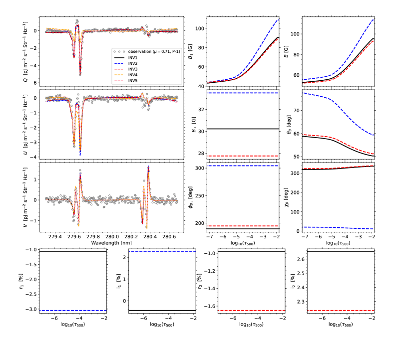
Figure 6: From top to bottom (top three panels in the left column), Stokes $Q$, $U$, and $V$ profiles, respectively. The open circles correspond to the temporally and spatially averaged observed Stokes profiles. From left to right and top to bottom (top three panels in the second and third columns), longitudinal component of the magnetic field, magnetic field strength, transversal component of the magnetic field, magnetic field inclination with respect to the local vertical, magnetic field azimuth in the plane perpendicular to the LOS, and magnetic field azimuth in the local vertical reference frame, respectively. From left to right (bottom row), the real part of the $Q=1$ tensor, the imaginary part of the $Q=1$ tensor, the real part of the $Q=2$ tensor, and the imaginary part of the $Q=2$ tensor characterizing the lack of axial symmetry, respectively. The solid black, and dashed blue, red, orange and pink curves correspond to the fit and inferred quantities from the inversion when including different combinations of horizontal inhomogeneity parameters as free parameters (see legend in the top left panel and see text for the description of the labels). The inferred quantities for the orange and pink cases are not shown because they do not fit the observations. This case corresponds to a region at the edge of the plage ($\mu=0.712$ in Fig. 1).

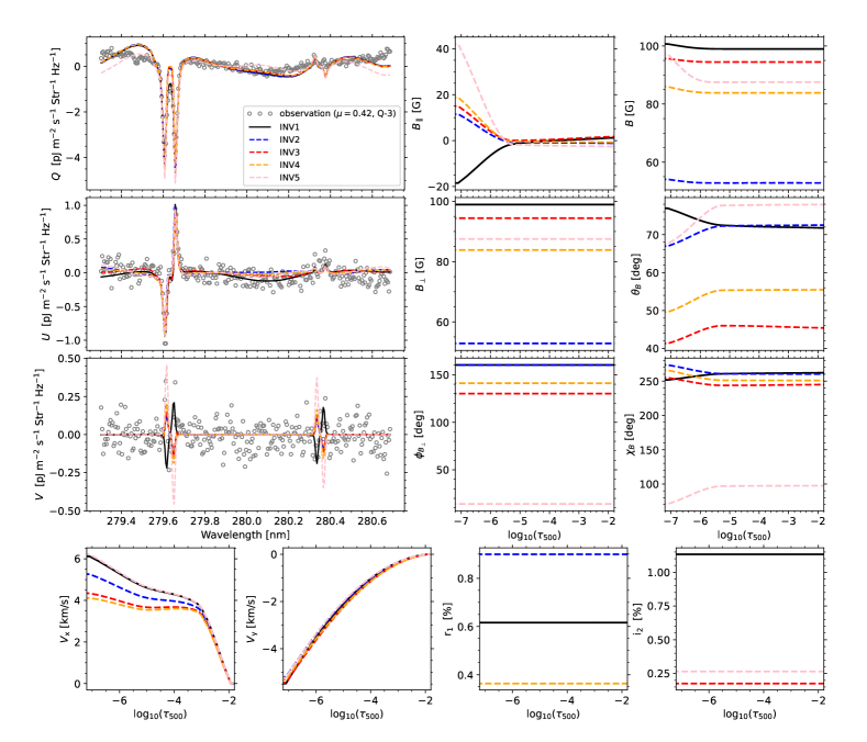
Figure 7: From top to bottom (top three panels in the left column), Stokes $Q$, $U$, and $V$ profiles, respectively. The open circles correspond to the temporally and spatially averaged observed Stokes profiles. From left to right and top to bottom (top three panels in the second and third columns), longitudinal component of the magnetic field, magnetic field strength, transversal component of the magnetic field, magnetic field inclination with respect to the local vertical, magnetic field azimuth in the plane perpendicular to the LOS, and magnetic field azimuth in the local vertical reference frame, respectively. From left to right (bottom row), horizontal component of the plasma velocity in the plane containing the LOS and the local vertical, horizontal component of the plasma velocity perpendicular to the same plane and the vertical, the real part of the $Q=1$ tensor, and the imaginary part of the $Q=2$ tensor characterizing the lack of axial symmetry, respectively. The solid black, and dashed blue, red, orange and pink curves correspond to the fit and inferred quantities from the inversion when including different combinations of horizontal inhomogeneity parameters in the inversion (see legend in the top left panel and see text for the description of the labels). This case corresponds to a region in the quiet Sun ($\mu=0.417$ in Fig. 1).

The $J^{\dagger}$ parameters in Eqs. (1) have a physical meaning, namely the symmetry breaking contribution from the presence of horizontal inhomogeneities in the solar atmosphere and macroscopic velocity gradients. The impact of the non-magnetic causes of symmetry breaking can be investigated through spectral synthesis calculations with codes like PORTA (Štěpán & Trujillo Bueno, 2013) that accounts for the effects of horizontal radiative transfer (e.g., Jaume Bestard et al., 2021). However, HanleRT-TIC is a 1D code, in which $J^{\dagger}$ was introduced as an ad-hoc parameter aimed at mimicking the missing physics. It is thus natural to ask if degeneracy and trade-off exist between the $J^{\dagger}$ contributions, both among themselves and with the magnetic field vector. The quick answer to this question is yes. The radiation field is calculated in the reference frame with the quantization axis along the local vertical and then transformed to the reference frame with the quantization axis along the magnetic field (Landi Degl’Innocenti & Landolfi, 2004). This transformation, which consists of a linear rotation with Euler angles, makes it possible that different sets of $J^{\dagger}$ transform into the same set of rotated tensors, especially given that the magnetic field direction is changing during the inversion steps. Moreover, it can also happen that some of the components of $J^{\dagger}$ impact the Stokes profiles in a similar (or opposite) way as some of the components of the magnetic field. Consequently, it is of critical importance to investigate how the degeneracy affects the inferred magnetic field vector. To this end, we have made a number of numerical experiments by applying HanleRT-TIC to some of CLASP2 Stokes profiles, considering different subsets of $J^{\dagger}$.

Figure 6 shows the result of several inversions of P-1 in Fig. 2 for different combinations of $J^{\dagger}$. The black solid curves show the inversion results obtained using the full $J^{\dagger}$ contributions (hereafter INV1), i.e., including both ${J^{\dagger}}^{2}_{1}$ and ${J^{\dagger}}^{2}_{2}$ with $r_{1}$, $i_{1}$, $r_{2}$, and $i_{2}$. The blue dashed curves show the inversion results including only ${J^{\dagger}}^{2}_{1}$ (hereafter INV2) with $r_{1}$ and $i_{1}$. The red dashed curves show the inversion results including only ${J^{\dagger}}^{2}_{2}$ (hereafter INV3) with $r_{2}$ and $i_{2}$. The orange dashed curves show the inversion results including only the real components of $J^{\dagger}$ (hereafter INV4) with $r_{1}$ and $r_{2}$. Finally, the pink dashed curves show the inversion results including only the imaginary components of $J^{\dagger}$ (hereafter INV5) with $i_{1}$ and $i_{2}$.

INV1, INV2, and INV3 provide good fits to the observations, while those of INV4 and INV5 clearly do not (and thus the inferred model atmospheres are not shown in Fig. 6). The three good fits return rather similar $B_{\parallel}$, $B_{\perp}$, and $B$, within a few gauss. However, the inferred $\phi_{B_{\perp}}$ shows significant differences. INV1 and INV3 return $\sim 190^{\circ}$, while INV3 returns $\sim 305^{\circ}$. If we look at the directions in the local reference frame, we find that the inclinations $\theta_{B}$ are relatively similar, within 10–20 degrees. A significant difference is found in the azimuth $\chi_{B}$, for which INV1 and INV3 return about $320^{\circ}$ (or $-40^{\circ}$) and INV2 returns about $20^{\circ}$. This discrepancy is likely due to intrinsic ambiguities of the Hanle effect. In contrast to the $180^{\circ}$ ambiguity characteristic of the Zeeman effect in the LOS reference frame, the ambiguity of the Hanle effect is related to the magnetic field vector in the local vertical frame. Analyzing this ambiguity for the Mg II k line is more complicated due to the strong impact of the MO and PRD effects on the linear polarization in the wings. In essence, the ambiguity of the Hanle effect consists on different combinations of $\theta_{B}$ and $\chi_{B}$ resulting in the same $Q$ and $U$. Even with these ambiguities, the inversions still confirms a $B_{\parallel}$ of about 45$\pm$5 G in the middle and upper chromosphere and a $B_{\perp}$ of about 30$\pm$4 G. Both $\phi_{B_{\perp}}$ and $\chi_{B}$ are affected by ambiguities. We also note that the inferred magnetic field vector is very similar between INV1 and INV3. The difference in the inferred values is much more important for $J^{\dagger}$, showing the degeneracy between the different components. INV3 returns larger values to compensate for the lack of ${J^{\dagger}}^{2}_{1}$, while INV2 returns larger values to compensate for the lack of ${J^{\dagger}}^{2}_{2}$.

Figure 7 shows the result of the same test for Q-2 in Fig. 5. INV1, INV3, INV4, and INV5 return a $B_{\perp}$ around 90 G, but INV2 returns about 50 G instead. The inferred $B_{\parallel}$ shows some differences, especially in the uppermost layers of the model, with INV1 returning about -20 G in the upper chromosphere, INV2, INV3, and INV4 about 20 G, and INV5 about 40 G. However, among all the inversions only INV1 can fit the Stokes $Q$ signal of the Mg II k line at its center. The other inversions could either get stuck in a local minimum or they could lack the degrees of freedom in $J^{\dagger}$ necessary to correctly fit the observation. In this case we also find the ambiguity in $\phi_{B_{\perp}}$ and $\chi_{B}$. All inversions are able to successfully fit the antisymmetric Stokes $U$ profile in the k line, returning an almost identical stratification of $v_{y}$ and similar stratifications of $v_{x}$. All of them retrieve an almost constant $v_{x}$ in the chromosphere and about a change of 5 km/s between lower and upper chromosphere in $v_{y}$. This is a confirmation of the $v_{y}$ stratification being the responsible of the antisymmetric shape of the Stokes $U$ profile in the Mg II k line.

We have performed the same test for Q-3 and Q-4 in Figs. 3–4, respectively, and the results can be found in the Appendix, in Figs. B.1–B.2. Our tests confirm the degeneracy between the ${J^{\dagger}}^{2}_{1}$ and ${J^{\dagger}}^{2}_{2}$. The inferred $B_{\parallel}$, $B_{\perp}$, and $B$ are similar within a few gauss, while $\phi_{B_{\perp}}$ and $\chi_{B}$ show differences likely due to the Hanle-effect ambiguities.

6 Summary and conclusions

While the intensity of the Mg II h & k lines allows us to infer information on the thermodynamic and dynamic properties of the solar chromosphere, their polarization signals encode information on the magnetic field all the way up from the upper photosphere to almost the base of the corona. The polarization in these strong resonance lines result from the joint action of scattering processes and the Hanle, Zeeman, and MO effects caused by the presence of magnetic fields. In particular, a rigorous modeling of their linear polarization signals requires solving the non-LTE 3D radiative transfer problem accounting for the radiatively induced atomic level polarization, PRD effects, and quantum interference between the magnetic sublevels pertaining to their upper $J$-levels, a very challenging unsolved problem, although some progress toward this goal has been recently made (Benedusi et al., 2023). The fact that the solar atmosphere is horizontally inhomogeneous and dynamic implies that the horizontal radiative transfer can break the axial symmetry of the radiation field that pumps the atoms at each spatial point within the atmospheric plasma, without the need of any inclined magnetic field. Therefore, in general, we have magnetic and non-magnetic causes of axial symmetry breaking.

Our HanleRT-TIC solves the radiative transfer problem taking into account all the above-mentioned mechanisms (i.e., PRD, $J$-state interference, Hanle, Zeeman and MO effects), but assuming 1D plane-parallel geometry (i.e., ignoring the effects of horizontal radiative transfer). In order to take into account in our Stokes inversions the possibility of non-magnetic causes of axial symmetry breaking (e.g., because of the presence of horizontal inhomogeneities in the temperature and density of the plasma), we have introduced in HanleRT-TIC ad-hoc components in the radiation field tensor that quantifies the axial symmetry breaking of the pumping radiation field. In this paper we have shown that such $J^{\dagger}$ contributions, which are additional Stokes inversion parameters, allow us to successfully fit a variety of Stokes profiles from the CLASP2 observations. For demonstrative purposes, we selected four representative types of the variety of CLASP2 Stokes profiles, including a location in the plage target (P-1, where Stokes-$V$ is significant but Stokes $Q$ and $U$ are negligible in the far wings) and three locations (Q-1, Q-2, and Q-3) in the quiet Sun target. At Q-1, Stokes $Q$ is significant in the far wings but Stokes $U$ is negligible, at Q-2 both Stokes $Q$ and $U$ are above the noise level, and at Q-3 we find antisymmetric Stokes $U$ profiles around the center of the k line.

We have found that the inclusion of $J^{\dagger}$ is necessary for fitting some of the CLASP2 Stokes profiles (P-1 and Q-2). In addition, we have identified a clear degeneracy between ${J^{\dagger}}^{2}_{1}$ and ${J^{\dagger}}^{2}_{2}$. It is important to emphasize that these ad-hoc contributions to the radiation field tensors are accounted for in a 3D forward solver (Štěpán & Trujillo Bueno, 2013; Benedusi et al., 2023) and for some lines can be estimated from the continuum illumination (Zeuner et al., 2020), although this method would not be suitable for the Mg II h & k lines. In order to address this challenge in an inversion a numerical code is in development following the guidelines in Štěpán et al. (2022), but the methodology is restricted, in principle, to spectral lines in the complete frequency redistribution regime (i.e., without PRD effects).

Interestingly, we have found that a gradient in the component of the horizontal velocity perpendicular to the plane containing the local vertical and the LOS ($v_{y}$) is needed to produce and fit one of our selected sets of Stokes profiles, namely the one showing an antisymmetric Stokes $U$ profile around the Mg II k line center. A difference of about 5 km/s between ${\rm log_{10}}(\tau_{500})=-7.0$ and -3.0 is found in the inversion of this Stokes profile, shown in Fig. 5. It is noteworthy that this kind of profile is only observed at a few positions along the CLASP2 slit. This suggests that in the quiet Sun chromosphere the gradient of $v_{y}$ is, generally, smaller than this value.

By performing several inversions with different subsets of $J^{\dagger}$ as free parameters, we have studied the degeneracy we have identified among the $J^{\dagger}$ components themselves, and with the magnetic field vector. For the four analyzed types of Stokes profiles, $B_{\parallel}$, $B_{\perp}$, and $B$ are found within a few gauss, typically $\pm 10$ G for all inversions (when they are able to fit the observations at all). The differences in $\theta_{B}$, $\phi_{B_{\perp}}$, and $\chi_{B}$ are more significant and they could be due to the ambiguities of the Hanle effect. Moreover, the lack of clear circular polarization signals, as in Q-1 and Q-2, favors a wider range of compatible solutions. The analysis of P-1 shown in Fig. 6 is indicative of how the access to circular polarization signals allows a much better constrain of $B_{\parallel}$ and, consequently, of the magnetic field vector, except for the ambiguities in the azimuths.

We have demonstrated that HanleRT-TIC is able to infer the vector magnetic field of the solar chromosphere from the Stokes profiles of the Mg II h & k lines, including the complex physical ingredients that are needed for their modeling. For example, in the quiet region pixels, where no circular polarization signal is detected, the magnetic field strength in the upper chromosphere varies between 1 and 20 gauss.

Of course, the accuracy of the retrieved magnetic field vector is limited by the polarimetric accuracy of the observations. Moreover, the heavy computational requirement of these non-LTE Stokes inversions severely limits its applicability to a large dataset. A faster inversion may be possible by applying clustering methods to select representative profiles (Sainz Dalda et al., 2019), by training convolutional neural networks to speed-up the computation of response functions (Centeno et al., 2022), or by extending other machine learning techniques (Vicente Arévalo et al., 2022; Asensio Ramos et al., 2023) to the more general non-LTE problem with atomic polarization.

Finally, we find it important to emphasize again that the results of the previous works on the analysis of the CLASP2 data (Ishikawa et al., 2021; Li et al., 2023; Afonso Delgado et al., 2023) and those of the present investigation highlight the potential of a new space mission with CLASP2-like capabilities for the study of the magnetic field in the solar chromosphere.

Appendix A Spatial average of the Stokes profiles

Figure A.1 shows the spatially averaged profile at $\mu=0.712$ (P-1, see section 4), as well as the Stokes profiles for the three individual pixels of the observation included in the average.

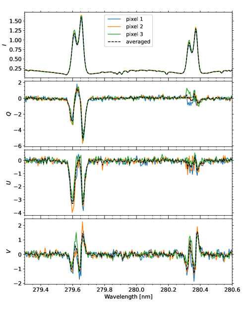
Figure A.1: From top to bottom, the intensity $I$ and Stokes $Q$, $U$, and $V$ profiles for the spatial average at $\mu=0.712$ (dashed black curve; see Fig. 2). The colored solid curves show the profiles for the individual pixels included in the average. The y axis units are the same as those in Fig. 2.

Appendix B Degeneracy tests

In Figs. B.1 and B.2 we show the degeneracy analysis (see Sect. 5) of the profiles in Figs. 3 and 4, respectively. As with the results shown in Sect. 5, the inferred $B_{\parallel}$, $B_{\perp}$, and $B$ are usually within a few gauss. However, noticeable differentces are found for $\phi_{B_{\perp}}$, $\theta_{B}$, and $\chi_{B}$, possibly due to the ambiguities in the Hanle effect.

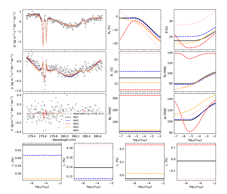
Figure B.1: Same as Fig. 6, but for a region in the quiet Sun with $\mu=0.563$ (see Fig. 1).

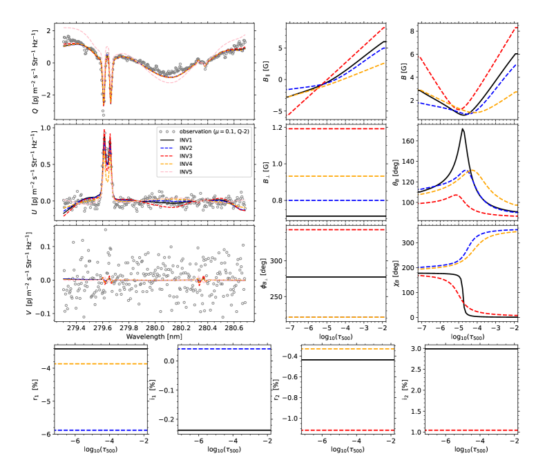
Figure B.2: Same as Fig. 6, but for a region in the quiet Sun with $\mu=0.101$ (see Fig. 1).

References

- Afonso Delgado et al. (2023) Afonso Delgado, D., del Pino Alemán, T., & Trujillo Bueno, J. 2023, ApJ, 954, 218, doi: 10.3847/1538-4357/ace4c8
- Alsina Ballester et al. (2016) Alsina Ballester, E., Belluzzi, L., & Trujillo Bueno, J. 2016, ApJ, 831, L15, doi: 10.3847/2041-8205/831/2/L15
- Asensio Ramos et al. (2023) Asensio Ramos, A., Cheung, M. C. M., Chifu, I., & Gafeira, R. 2023, Living Reviews in Solar Physics, 20, 4, doi: 10.1007/s41116-023-00038-x
- Asensio Ramos et al. (2008) Asensio Ramos, A., Trujillo Bueno, J., & Land i Degl’Innocenti, E. 2008, ApJ, 683, 542, doi: 10.1086/589433
- Belluzzi & Trujillo Bueno (2012) Belluzzi, L., & Trujillo Bueno, J. 2012, ApJ, 750, L11, doi: 10.1088/2041-8205/750/1/L11
- Benedusi et al. (2023) Benedusi, P., Riva, S., Zulian, P., et al. 2023, Journal of Computational Physics, 479, 112013, doi: 10.1016/j.jcp.2023.112013
- Centeno et al. (2022) Centeno, R., Flyer, N., Mukherjee, L., et al. 2022, ApJ, 925, 176, doi: 10.3847/1538-4357/ac402f
- de la Cruz Rodríguez & van Noort (2017) de la Cruz Rodríguez, J., & van Noort, M. 2017, Space Sci. Rev., 210, 109, doi: 10.1007/s11214-016-0294-8
- del Pino Alemán et al. (2016) del Pino Alemán, T., Casini, R., & Manso Sainz, R. 2016, ApJ, 830, L24, doi: 10.3847/2041-8205/830/2/L24
- del Pino Alemán et al. (2020) del Pino Alemán, T., Trujillo Bueno, J., Casini, R., & Manso Sainz, R. 2020, ApJ, 891, 91, doi: 10.3847/1538-4357/ab6bc9
- del Pino Alemán et al. (2018) del Pino Alemán, T., Trujillo Bueno, J., Štěpán, J., & Shchukina, N. 2018, ApJ, 863, 164, doi: 10.3847/1538-4357/aaceab
- del Toro Iniesta & Ruiz Cobo (2016) del Toro Iniesta, J. C., & Ruiz Cobo, B. 2016, Living Reviews in Solar Physics, 13, 4, doi: 10.1007/s41116-016-0005-2
- Fontenla et al. (1993) Fontenla, J. M., Avrett, E. H., & Loeser, R. 1993, ApJ, 406, 319, doi: 10.1086/172443
- Ishikawa et al. (2021) Ishikawa, R., Trujillo Bueno, J., del Pino Alemán, T., et al. 2021, Science Advances, 7, eabe8406, doi: 10.1126/sciadv.abe8406
- Ishikawa et al. (2023) Ishikawa, R., Trujillo Bueno, J., Alsina Ballester, E., et al. 2023, ApJ, 945, 125, doi: 10.3847/1538-4357/acb64e
- Jaume Bestard et al. (2021) Jaume Bestard, J., Trujillo Bueno, J., Štěpán, J., & del Pino Alemán, T. 2021, ApJ, 909, 183, doi: 10.3847/1538-4357/abd94a
- Lagg et al. (2017) Lagg, A., Lites, B., Harvey, J., Gosain, S., & Centeno, R. 2017, Space Sci. Rev., 210, 37, doi: 10.1007/s11214-015-0219-y
- Landi Degl’Innocenti & Landolfi (2004) Landi Degl’Innocenti, E., & Landolfi, M. 2004, Polarization in Spectral Lines, Vol. 307 (Dordrecht:KluwerAcademic), doi: 10.1007/978-1-4020-2415-3
- Li et al. (2022) Li, H., del Pino Alemán, T., Trujillo Bueno, J., & Casini, R. 2022, ApJ, 933, 145, doi: 10.3847/1538-4357/ac745c
- Li et al. (2023) Li, H., del Pino Alemán, T., Trujillo Bueno, J., et al. 2023, ApJ, 945, 144, doi: 10.3847/1538-4357/acb76e
- Manso Sainz & Trujillo Bueno (2011) Manso Sainz, R., & Trujillo Bueno, J. 2011, ApJ, 743, 12, doi: 10.1088/0004-637X/743/1/12
- Narukage et al. (2016) Narukage, N., McKenzie, D. E., Ishikawa, R., et al. 2016, in Society of Photo-Optical Instrumentation Engineers (SPIE) Conference Series, Vol. 9905, Space Telescopes and Instrumentation 2016: Ultraviolet to Gamma Ray, ed. J.-W. A. den Herder, T. Takahashi, & M. Bautz, 990508, doi: 10.1117/12.2232245
- Rachmeler et al. (2022) Rachmeler, L. A., Trujillo Bueno, J., McKenzie, D. E., et al. 2022, ApJ, 936, 67, doi: 10.3847/1538-4357/ac83b8
- Sainz Dalda et al. (2019) Sainz Dalda, A., de la Cruz Rodríguez, J., De Pontieu, B., & Gošić, M. 2019, ApJ, 875, L18, doi: 10.3847/2041-8213/ab15d9
- Song et al. (2018) Song, D., Ishikawa, R., Kano, R., et al. 2018, in Society of Photo-Optical Instrumentation Engineers (SPIE) Conference Series, Vol. 10699, Space Telescopes and Instrumentation 2018: Ultraviolet to Gamma Ray, ed. J.-W. A. den Herder, S. Nikzad, & K. Nakazawa, 106992W, doi: 10.1117/12.2313056
- Song et al. (2022) Song, D., Ishikawa, R., Kano, R., et al. 2022, Sol. Phys., 297, 135, doi: 10.1007/s11207-022-02064-8
- Trujillo Bueno & del Pino Alemán (2022) Trujillo Bueno, J., & del Pino Alemán, T. 2022, ARA&A, 60, 415, doi: 10.1146/annurev-astro-041122-031043
- Tsuzuki et al. (2020) Tsuzuki, T., Ishikawa, R., Kano, R., et al. 2020, in Society of Photo-Optical Instrumentation Engineers (SPIE) Conference Series, Vol. 11444, Society of Photo-Optical Instrumentation Engineers (SPIE) Conference Series, 114446W, doi: 10.1117/12.2562273
- Vicente Arévalo et al. (2022) Vicente Arévalo, A., Asensio Ramos, A., & Esteban Pozuelo, S. 2022, ApJ, 928, 101, doi: 10.3847/1538-4357/ac53b3
- Štěpán et al. (2022) Štěpán, J., del Pino Alemán, T., & Trujillo Bueno, J. 2022, A&A, 659, A137, doi: 10.1051/0004-6361/202142079
- Štěpán et al. (2024) —. 2024, arXiv e-prints, arXiv:2407.20926, doi: 10.48550/arXiv.2407.20926
- Štěpán & Trujillo Bueno (2013) Štěpán, J., & Trujillo Bueno, J. 2013, A&A, 557, A143, doi: 10.1051/0004-6361/201321742
- Zeuner et al. (2024) Zeuner, F., del Pino Alemán, T., Trujillo Bueno, J., & Solanki, S. K. 2024, ApJ, 964, 10, doi: 10.3847/1538-4357/ad26f9
- Zeuner et al. (2020) Zeuner, F., Manso Sainz, R., Feller, A., et al. 2020, ApJ, 893, L44, doi: 10.3847/2041-8213/ab86b8