A study on two-metric projection methods

1 Abstract

The two-metric projection method is a simple yet elegant algorithm proposed by Bertsekas in 1984 to address bound/box-constrained optimization problems. The algorithm’s low per-iteration cost and potential for using Hessian information makes it a favourable computation method for this problem class. However, its global convergence guarantee is not studied in the nonconvex regime. In our work, we first investigate the global complexity of such a method for finding first-order stationary solution. After properly scaling each step, we equip the algorithm with competitive complexity guarantees. Furthermore, we generalize the two-metric projection method for solving $\ell_{1}$-norm minimization and discuss its properties via theoretical statements and numerical experiments.

2 Introduction

In this work, we revisit the two-metric projection method proposed by Bertsekas [2] to solve the bound-constrained problem:

$$\begin{array}[]{*{2}{rl}}\min\;f(x)\quad\mbox{subject to}\quad x\geq 0\end{array}$$ (1)

where $f:\mathbb{R}^{n}\rightarrow\mathbb{R}$ is Lipschitz continuously differentiable and is bounded below by $f_{\text{low }}$ on the feasible region. Two-metric projection method is simple and elegant, but its global complexity guarantees are absent in literature. We observe that this traditional method finds an approximate first-order optimal point in $\mathcal{O}(\epsilon^{-3})$ iterations, which is suboptimal in literature [3]. By properly scaling the diagonal matrix, we equip the method with a worst-case complexity that matches the lower bound ($\mathcal{O}(\epsilon^{-2})$) of using first-order methods to solve this problem class. Moreover, we try to generalize the method and propose a two-metric adaptive projection method for the $\ell_{1}$-norm minimization,

$$\min\;\psi(x)\triangleq f(x)+\gamma\|x\|_{1}.$$ (2)

We show that our method is well-defined and decreases the value of the objective function at each iteration $k$ for which $x_{k}$ is not a critical point. For (2), inexact proximal-Newton-type methods, or successive quadratic approximation (SQA) methods [4], are widely used for their superlinear convergence in terms of iterations. A key difference between the two-metric adaptive projection and these methods is the per-iteration cost: in each iteration, SQA needs to find approximate solutions to regularized quadratic programs, while our method at worst needs to solve a linear equation - the Newton system and compute a single cheap adaptive projection step. Preliminary numerical experiments verify the asymptotic superlinear convergence of the two-metric adaptive projection method when employing Hessian.

3 First-order optimal point

We can write first-order optimality conditions for (1), (also known as stationarity conditions) at a point $\bar{x}$ as follows:

$$\partial f\left(\bar{x}\right)/\partial x^{i}=0\quad\text{if}\quad\bar{x}^{i}>0,\quad i=1,\ldots,n,$$ (3)

$$\partial f\left(\bar{x}\right)/\partial x^{i}\geq 0\quad\text{if}\quad\bar{x}^{i}=0,\quad i=1,\ldots,n.$$

3.1 Approximate first-order optimal points

Next, we define $\epsilon$-approximate first-order optimal points ($\epsilon$-1o).

Definition 1

For $\epsilon>0$, $\bar{x}$ is an $\epsilon$-1o point of (1), if $\bar{x}\geq 0$ and

$$\|S\nabla f(\bar{x})\|\leq\epsilon,\quad(\nabla f(\bar{x}))_{i}\geq-\epsilon,$$ (4)

where $S$ is a diagonal matrix such that $S[i,i]=\min\left\{\bar{x}^{i},1\right\}$ if $\bar{x}^{i}\geq 0,(\nabla f(\bar{x}))_{i}>0$; $S[i,i]=1$ otherwise.

Definition 1 is motivated by the first-order optimal conditions of (1). In fact, if we let $\epsilon$ = 0, then 0-1o satisfies (3) exactly. The following lemma further justifies Definition 1 and our purpose to find an $\epsilon$-1o given small $\epsilon$.

Lemma 1

Consider problem (1), suppose that we have a positive scalar sequence $\left\{\epsilon_{k}\right\}$ with $\epsilon_{k}\to 0$ and vector sequence $\left\{x_{k}\right\}$ with $x_{k}\geq 0$ and $x_{k}\to x_{*}$ such that $x_{k}$ is $\epsilon_{k}$-1o according to Definition 1. Then $x_{*}$ satisfies first-order optimal conditions (3).

Proof

Denote diagonal matrix $S_{k}$ where coorespond to $S$ in Definition 1 with $x=x_{k},\epsilon=\epsilon_{k}$. Our claim that $x_{*}$ satisfies (3) is a consequence of the following three observations.

1. Feasibility of $x_{*}$ follows from closedness of $\Omega$.

2. $\forall i,k$, $\nabla_{i}f(x_{k})\geq-\epsilon_{k}$. By taking limits, we have $\nabla_{i}f(x_{*})\geq 0$

3. We claim that if $x_{*}^{i}>0$, we must have $\nabla_{i}f(x_{*})=0$. Assume the contrary, if $\nabla_{i}f(x_{*})>0$, there exist a $K$, for all $k\geq K$ we have $\nabla_{i}f(x_{k})>0$ and $x_{k}^{i}>\frac{1}{2}x_{*}^{i}>0$, then $\forall k\geq K$

   $$\min\left\{\frac{1}{2}x_{*}^{i},1\right\}\nabla_{i}f(x_{k})<|\min\left\{x_{k}^{i},1\right\}\nabla_{i}f(x_{k})|\leq\|S_{k}\nabla f(x_{k})\|\leq\epsilon_{k}.$$

   By taking limits, we have $\nabla_{i}f(x_{*})=0$, which is contradicting with $\nabla_{i}f(x_{*})>0$.

Overall, $x^{*}$ satisfies (3).

4 Two-metric projection

The two-metric projection method for solving (1) is as follows:

$$x_{k+1}:=\mathcal{P}\left(x_{k}-\alpha_{k}D_{k}g_{k}\right),\quad\forall k\geq 0,$$

where $\mathcal{P}$ denotes Euclidean projection onto the feasible region, $\alpha_{k}>0$ is the stepsize, $g_{k}\triangleq\nabla f\left(x_{k}\right)$. $D_{k}$ is a symmetric positive definite matrix in $\mathbb{R}^{n\times n}$. Define

$$p_{k}\triangleq D_{k}g_{k},I_{k}^{+}\triangleq\left\{i\mid 0\leq x_{k}^{i}\leq\epsilon_{k},\;g_{k}^{i}>0\right\},\;I_{k}^{-}\triangleq[1,\ldots,n]\backslash I_{k}^{+},$$

where $\epsilon_{k}=\min\left\{\epsilon,\omega_{k}\right\}$, $\omega_{k}=\|x_{k}-P(x_{k}-M\nabla f(x_{k}))\|$, $\epsilon>0$ is a fixed tolerance and $M$ is a fixed diagonal positive definite matrix. We suppose that $D_{k}$ is diagonal w.r.t. $I_{k}^{+}$ , i.e.,

$$D_{k}[i,j]=0,\quad\forall i\in I_{k}^{+},j\neq i.$$ (5)

Denote $x_{k}(\alpha)\triangleq P\left(x_{k}-\alpha p_{k}\right),\forall\alpha>0$. Let $\bar{g}_{k}$ and $\bar{p}_{k}$ be the subvector of $g_{k}$ and $p_{k}$ w.r.t index set $I_{k}^{-}$ , and $\bar{D}_{k}$ be the submatrix of $D_{k}$ and w.r.t. $I_{k}^{-}\times I_{k}^{-}$. $S_{k}$ is the diagonal matrix which corresponds to $I^{+},I^{-}$, and $S$ in Definition 1 with $x=x_{k},s=s_{k}$ and $\epsilon$. Then the algorithm can be formally stated as follows.

Input: tolerance $\epsilon>0$, step acceptance parameter $\sigma\in(0,1)$, backtracking parameter $\beta\in(0,1)$ and initial feasible point $x_{0}$. Let $k=0$.

while $\|S_{k}\nabla f(x_{k})\|>\epsilon$ do

       Find:

$$m_{k}\triangleq\min\left\{m\in\mathbb{N}\Bigg{|}f\left(x_{k}\right)-f\left(x_{k}\left(\beta^{m}\right)\right)\geq\sigma\left\{\beta^{m}\sum_{i\notin I_{k}^{+}}g_{k}^{i}p_{k}^{i}+\sum_{i\in I_{k}^{+}}g_{k}^{i}(x_{k}^{i}-x_{k}^{i}\left(\beta^{m}\right))\right\}\right\}$$

      Let $\alpha_{k}=\beta^{m_{k}}$, $x_{k+1}=x_{k}(\alpha_{k})$.

      Let $k=k+1$.

end while

Output: $x_{k}$

Algorithm 1 Two-metric projection

Remark 1

We do not need to consider if $(\nabla f(x_{k}))_{i}<-\epsilon$ or not in the Algorithm 1, since if $(\nabla f(x_{k}))_{i}<-\epsilon$, then

$$\|S_{k}\nabla f(x_{k})\|\geq|(\nabla f(\bar{x}))_{i}|>\epsilon$$

Complexity of Algorithm 1 is revealed in the following theorem.

Theorem 4.1

Consider Algorithm 1. Suppose that $\lambda_{\min}\|z\|^{2}\leq z^{T}D_{k}z\leq\lambda_{\max}\|z\|^{2}$, for all $z\in\mathbb{R}^{n}$ and $k\geq 0$. $\left\|g_{k}\right\|\leq G,\forall k\geq 0$. Lipschitz constant for $\nabla f$ is $L$. Then $m_{k}<+\infty$ and the following holds: for any $0<\epsilon<1$, the algorithm will stop within $\mathcal{O}(\epsilon^{-3})$ number of iterations and output an $\epsilon$-1o $\bar{x}$ that satisfies Definition 1.

Remark 2

We suppress the proof of Theorem 4.1 due to page limit. Note that the best complexity of first-order methods for Lipschitz smooth function $f$ in literature is $\mathcal{O}(\epsilon^{-2})$. The reason to cause this gap is the possible small stepsize in the current form of two-metric projection. Motivated by this gap, we design a scaled two-metric projection method to enlarge the stepsize and improve the complexity guarantees.

5 Scaled two-metric projection

In this section, we apply an extended scaled version of the two-metric projection algorithm. The only difference between the scaled version and the traditional version is that we use a diagonal matrix to scale $D_{k}$. We update $x_{k+1}$ using:

$$x_{k+1}:=\mathcal{P}\left(x_{k}-\alpha_{k}S_{k}D_{k}S_{k}g_{k}\right),\quad\forall k\geq 0,$$

Where $S_{k}$ is defined as follows:

$$S_{k}[i,i]=\min\left\{x_{k}^{i},1\right\},\text{ if }g_{k}^{i}>0;\quad S_{k}[i,i]=1\text{, otherwise. }$$ (6)

Define $p_{k}\triangleq S_{k}D_{k}S_{k}g_{k}$. The Algorithm is formally the same as Algorithm 1 with only different $p_{k}$. The following theorem shows an improved complexity guarantee for this algorithm.

Theorem 5.1

Consider Algorithm 2. Suppose that $\lambda_{\min}\|z\|^{2}\leq z^{T}D_{k}z\leq\lambda_{\max}\|z\|^{2}$, for all $z\in\mathbb{R}^{n}$ and $k\geq 0$. $\left\|g_{k}\right\|\leq G,\forall k\geq 0$. Lipschitz constant for $\nabla f$ is $L$. Then $m_{k}<+\infty$ and the following holds. For any $0<\epsilon<1$, the algorithm will stop within $\left\lceil\frac{(f(x_{0})-f_{\text{low}})\max\left\{4\lambda_{\max}G,\frac{2L\lambda_{\max}}{1-\sigma},2\beta\lambda_{\text{min}}\right\}}{\sigma\beta\lambda_{\text{min}}\epsilon^{2}}\right\rceil$ number of iterations and output an $\bar{x}$ that satisfies Definition 1.

Proof

First we show that $m_{k}<+\infty,\forall k\geq 0$. Denote $I_{k}^{p+}\triangleq\left\{i\mid p_{k}^{i}>0,g_{k}^{i}\leq 0\right\}$, $s_{k}^{i}\triangleq S_{k}[i,i]$. Note that $I_{k}^{p+}\in I_{k}^{-}$ and $I_{k}^{-}\setminus I_{k}^{p+}=\left\{i\mid 0\leq x_{k}^{i}\leq\epsilon_{k},g_{k}^{i}\leq 0,p_{k}^{i}\leq 0\right\}\cup\left\{i\mid x_{k}^{i}>\epsilon_{k},g_{k}^{i}>0\right\}\cup\left\{i\mid x_{k}^{i}>\epsilon_{k},p_{k}^{i}\leq 0\right\}$. If $\forall\alpha>0$ such that

$$\alpha\leq\min_{i\in\left\{i\in I_{k}^{-}\mid g_{k}^{i}>0,p_{k}^{i}>0\right\}}\left\{\frac{x_{k}^{i}}{p_{k}^{i}}\right\},$$ (7)

we have the following properties:

$$x_{k}^{i}(\alpha)=x_{k}^{i}-\alpha p_{k}^{i},\quad\forall i\in I_{k}^{-}\setminus I_{k}^{p+},$$ (8)

$$g_{k}^{i}\leq 0,x_{k}^{i}(\alpha)=\left[x_{k}^{i}-\alpha p_{k}^{i}\right]_{+}\geq x_{k}^{i}-\alpha p_{k}^{i}\Longrightarrow g_{k}^{i}(x_{k}^{i}-\alpha p_{k}^{i}-x_{k}^{i}(\alpha))\geq 0,\quad\forall i\in I_{k}^{p+},$$ (9)

Therefore,

$$\sum_{i\in I_{k}^{-}}g_{k}^{i}\left(x_{k}^{i}(\alpha)-x_{k}^{i}\right)$$ (10)

$$= \sum_{i\in I_{k}^{-}\setminus I_{k}^{p+}}g_{k}^{i}\left(x_{k}^{i}(\alpha)-x_{k}^{i}\right)+\sum_{i\in I_{k}^{p+}}g_{k}^{i}\left(x_{k}^{i}(\alpha)-x_{k}^{i}\right)$$

$$= \sum_{i\in I_{k}^{-}\setminus I_{k}^{p+}}g_{k}^{i}\left(-\alpha p_{k}^{i}\right)+\sum_{i\in I_{k}^{p+}}g_{k}^{i}\left(x_{k}^{i}(\alpha)-x_{k}^{i}+\alpha p_{k}^{i}\right)+\sum_{i\in I_{k}^{p+}}g_{k}^{i}\left(-\alpha p_{k}^{i}\right)\leq\sum_{i\in I_{k}^{-}}g_{k}^{i}\left(-\alpha p_{k}^{i}\right)$$

Since $\forall\alpha>0$, we have:

$$x_{k}^{i}(\alpha)=\left[x_{k}^{i}-\alpha p_{k}^{i}\right]_{+}\geq x_{k}^{i}-\alpha p_{k}^{i}\Longrightarrow x_{k}^{i}-x_{k}^{i}(\alpha)\leq\alpha p_{k}^{i},\quad\forall i\in I_{k}^{+},$$ (11)

$$0\leq p_{k}^{i}=s_{k}^{i}D_{k}\left[i,i\right]s_{k}^{i}g_{k}^{i}\leq D_{k}\left[i,i\right]g_{k}^{i}\leq\lambda_{\text{max}}g_{k}^{i}\Longrightarrow 0\leq x_{k}^{i}-x_{k}^{i}(\alpha),\quad\forall i\in I_{k}^{+},$$ (12)

$$\left|x_{k}^{i}-x_{k}^{i}(\alpha)\right|\leq\alpha\left|p_{k}^{i}\right|.$$ (13)

Then,

$$\sum_{i\in I_{k}^{+}}\left(x_{k}^{i}(\alpha)-x_{k}^{i}\right)^{2}\leq\sum_{i\in I_{k}^{+}}\alpha p_{k}^{i}(x_{k}^{i}-x_{k}^{i}(\alpha))\leq\alpha\lambda_{\text{max}}\sum_{i\in I_{k}^{+}}g_{k}^{i}(x_{k}^{i}-x_{k}^{i}(\alpha)).$$ (14)

Note that $\|\bar{S}_{k}\|\leq 1$ and $\forall z\in\mathbb{R}^{n},D\in\mathbb{S}^{n}_{++}$ we have:

$$\|Dz\|^{2}=z^{T}D^{2}z=z^{T}D^{\frac{1}{2}}DD^{\frac{1}{2}}z=(D^{\frac{1}{2}}z)^{T}D(D^{\frac{1}{2}}z)\leq\lambda_{\text{max}}\|D^{\frac{1}{2}}z\|^{2}=\lambda_{\text{max}}z^{T}Dz$$ (15)

Therefore,

$$\sum_{i\in I_{k}^{-}}\left(x_{k}^{i}(\alpha)-x_{k}^{i}\right)^{2}\leq\sum_{i\in I_{k}^{-}}(\alpha p_{k}^{i})^{2}=\alpha^{2}\|\bar{p}_{k}\|^{2}=\alpha^{2}\left\|\bar{S}_{k}\bar{D}_{k}\bar{S}_{k}\bar{g}_{k}\right\|^{2}$$ (16)

$$\leq \alpha^{2}\|\bar{S}_{k}\|^{2}\left\|\bar{D}_{k}\bar{S}_{k}\bar{g}_{k}\right\|^{2}\leq\alpha^{2}\left\|\bar{D}_{k}\bar{S}_{k}\bar{g}_{k}\right\|^{2}\leq\alpha^{2}\lambda_{\max}\bar{g}_{k}^{T}\bar{S}_{k}\bar{D}_{k}\bar{S}_{k}\bar{g}_{k}$$

$$= \alpha^{2}\lambda_{\max}\bar{g}_{k}^{T}\bar{p}_{k}=\alpha^{2}\lambda_{\text{max}}\sum_{i\in I_{k}^{-}}g_{k}^{i}p_{k}^{i}.$$

Since $\forall i\in\left\{i\in I_{k}^{-}\mid g_{k}^{i}>0,p_{k}^{i}>0\right\}$, we have:

$$0<p_{k}^{i}=s_{k}^{i}(D_{k}S_{k}g_{k})^{i}=\min\left\{x_{k}^{i},1\right\}(D_{k}S_{k}g_{k})^{i}\leq x_{k}^{i}\|D_{k}S_{k}g_{k}\|_{\infty}$$ (17)

$$\leq x_{k}^{i}\|D_{k}S_{k}g_{k}\|_{2}\leq x_{k}^{i}\|D_{k}\|_{2}\|S_{k}\|_{2}\|g_{k}\|_{2}\leq x_{k}^{i}\lambda_{\text{max}}G$$

which indicates that,

$$\frac{x_{k}^{i}}{p_{k}^{i}}\geq\frac{1}{\lambda_{\text{max}}G},\quad\forall i\in\left\{i\in I_{k}^{-}\mid g_{k}^{i}>0,p_{k}^{i}>0\right\}.$$ (18)

Therefore, if $\alpha\leq\frac{1}{\lambda_{\text{max}}G}$, we have:

$$\alpha\leq\min_{i\in\left\{i\in I_{k}^{-}\mid g_{k}^{i}>0,p_{k}^{i}>0\right\}}\left\{\frac{x_{k}^{i}}{p_{k}^{i}}\right\}.$$

From Lipschitz continuity of $\nabla f$, we have that for any $\alpha$ satisfying $\alpha\leq\frac{1}{\lambda_{\text{max}}G}$,

$$f\left(x_{k}(\alpha)\right)-f\left(x_{k}\right) \leq g_{k}^{T}\left(x_{k}(\alpha)-x_{k}\right)+\frac{L}{2}\left\|x_{k}(\alpha)-x_{k}\right\|^{2}$$ (19)

$$\leq(\frac{\alpha^{2}\lambda_{\text{max}}L}{2}-\alpha)\sum_{i\in I_{k}^{-}}g_{k}^{i}p_{k}^{i}+(\frac{\alpha\lambda_{\text{max}}L}{2}-1)\sum_{i\in I_{k}^{+}}g_{k}^{i}(x_{k}^{i}-x_{k}^{i}(\alpha)).$$

If $\alpha$ satisfies $\alpha\leq\frac{2(1-\sigma)}{L\lambda_{\max}}$, then we have:

$$f\left(x_{k}\right)-f\left(x_{k}\left(\alpha\right)\right)\geq\sigma\left\{\alpha\sum_{i\notin I_{k}^{+}}g_{k}^{i}p_{k}^{i}+\sum_{i\in I_{k}^{+}}g_{k}^{i}(x_{k}^{i}-x_{k}^{i}\left(\alpha\right))\right\}.$$ (20)

Let $\bar{\alpha}\triangleq\min\left\{\frac{1}{\lambda_{\max}G},\frac{2(1-\sigma)}{L\lambda_{\max}}\right\}$. Due to the definition of $m_{k}$, $m_{k}\leq\min\left\{m\in\mathbb{N}\mid\beta^{m}\leq\bar{\alpha}\right\}$ and $\beta^{m_{k}-1}>\bar{\alpha}$. Thus $m_{k}<+\infty$. This further indicates that

$$\alpha_{k}/\beta=\beta^{m_{k}-1}>\bar{\alpha}\Longrightarrow\alpha_{k}>\bar{\alpha}\beta.$$ (21)

Next, we consider the iteration complexity of Algorithm 1.

$$\|S_{k}\nabla f(x_{k})\|>\epsilon\Longleftrightarrow\|S_{k}\nabla f(x_{k})\|^{2}>\epsilon^{2}\Longrightarrow\sum_{i\in I_{k}^{+}}(s_{k}^{i}g_{k}^{i})^{2}>\frac{\epsilon^{2}}{2}\text{ or }\sum_{i\in I_{k}^{-}}(s_{k}^{i}g_{k}^{i})^{2}>\frac{\epsilon^{2}}{2}$$ (22)

If

$$\sum_{i\in I_{k}^{+}}(s_{k}^{i}g_{k}^{i})^{2}>\frac{\epsilon^{2}}{2}\Longleftrightarrow\sum_{i\in I_{k}^{+}}(x_{k}^{i}g_{k}^{i})^{2}>\frac{\epsilon^{2}}{2}\Longrightarrow\sum_{\begin{subarray}{c}i\in I_{k}^{+}\\ x_{k}^{i}-\alpha p_{k}^{i}\geq 0\end{subarray}}(x_{k}^{i}g_{k}^{i})^{2}>\frac{\epsilon^{2}}{4}\text{ or }\sum_{\begin{subarray}{c}i\in I_{k}^{+}\\ x_{k}^{i}-\alpha p_{k}^{i}<0\end{subarray}}(x_{k}^{i}g_{k}^{i})^{2}>\frac{\epsilon^{2}}{4}$$ (23)

Then,

$$\sum_{i\in I_{k}^{+}}g_{k}^{i}(x_{k}^{i}-x_{k}^{i}\left(\alpha\right))= \sum_{\begin{subarray}{c}i\in I_{k}^{+}\\ x_{k}^{i}-\alpha p_{k}^{i}\geq 0\end{subarray}}\alpha p_{k}^{i}g_{k}^{i}+\sum_{\begin{subarray}{c}i\in I_{k}^{+}\\ x_{k}^{i}-\alpha p_{k}^{i}<0\end{subarray}}x_{k}^{i}g_{k}^{i}$$ (24)

$$= \sum_{\begin{subarray}{c}i\in I_{k}^{+}\\ x_{k}^{i}-\alpha p_{k}^{i}\geq 0\end{subarray}}\alpha(x_{k}^{i}g_{k}^{i})^{2}D_{k}[i,i]+\sum_{\begin{subarray}{c}i\in I_{k}^{+}\\ x_{k}^{i}-\alpha p_{k}^{i}<0\end{subarray}}x_{k}^{i}g_{k}^{i}$$

$$\geq \sum_{\begin{subarray}{c}i\in I_{k}^{+}\\ x_{k}^{i}-\alpha p_{k}^{i}\geq 0\end{subarray}}\alpha\lambda_{\text{min}}(x_{k}^{i}g_{k}^{i})^{2}+\sqrt{\sum_{\begin{subarray}{c}i\in I_{k}^{+}\\ x_{k}^{i}-\alpha p_{k}^{i}<0\end{subarray}}(x_{k}^{i}g_{k}^{i})^{2}}$$

$$\geq \min\left\{\bar{\alpha}\beta\lambda_{\text{min}}\frac{\epsilon^{2}}{4},\frac{\epsilon}{2}\right\}\stackrel{{\scriptstyle\epsilon<1}}{{\geq}}\min\left\{\bar{\alpha}\beta\lambda_{\text{min}}\frac{\epsilon^{2}}{4},\frac{\epsilon^{2}}{2}\right\}$$

Else,

$$\sum_{i\in I_{k}^{-}}(s_{k}^{i}g_{k}^{i})^{2}>\frac{\epsilon^{2}}{2}$$ (25)

Then,

$$\alpha\sum_{i\notin I_{k}^{+}}g_{k}^{i}p_{k}^{i}=\alpha\bar{g}_{k}^{T}\bar{p}_{k}=\alpha\bar{g}_{k}^{T}\bar{S}_{k}\bar{D}_{k}\bar{S}_{k}\bar{g}_{k}\geq\alpha\lambda_{\text{min}}\|\bar{S}_{k}\bar{g}_{k}\|^{2}\geq\bar{\alpha}\beta\lambda_{\text{min}}\|\bar{S}_{k}\bar{g}_{k}\|^{2}\geq\bar{\alpha}\beta\lambda_{\text{min}}\frac{\epsilon^{2}}{2}$$ (26)

Therefore, if $\|S_{k}\nabla f(x_{k})\|>\epsilon$ hold, from (22)(26)(28) we have:

$$f\left(x_{k}\right)-f\left(x_{k}\left(\alpha\right)\right)\geq \sigma\left\{\alpha\sum_{i\notin I_{k}^{+}}g_{k}^{i}p_{k}^{i}+\sum_{i\in I_{k}^{+}}g_{k}^{i}(x_{k}^{i}-x_{k}^{i}\left(\alpha\right))\right\}$$ (27)

$$\geq \sigma\min\left\{\frac{\bar{\alpha}\beta\lambda_{\text{min}}}{4},\frac{1}{2}\right\}\epsilon^{2}$$

Suggest that the algorithm will stop within $K$ number of iterations, then,

$$f(x_{0})-f_{\text{low}}\geq\sum_{k=0}^{K-1}f\left(x_{k}\right)-f\left(x_{k}\left(\alpha\right)\right)=f(x_{0})-f(x_{K})\geq K\sigma\min\left\{\frac{\bar{\alpha}\beta\lambda_{\text{min}}}{4},\frac{1}{2}\right\}\epsilon^{2}$$ (28)

This further indicates that,

$$K\leq\frac{f(x_{0})-f_{\text{low}}}{\sigma\min\left\{\frac{\bar{\alpha}\beta\lambda_{\text{min}}}{4},\frac{1}{2}\right\}\epsilon^{2}}=\frac{(f(x_{0})-f_{\text{low}})\max\left\{4\lambda_{\max}G,\frac{2L\lambda_{\max}}{1-\sigma},2\beta\lambda_{\text{min}}\right\}}{\sigma\beta\lambda_{\text{min}}\epsilon^{2}}$$ (29)

6 Generalize the method for $\ell_{1}$-norm regularization problem

We consider the $\ell_{1}$-norm regularization problem:

$$\min\psi(x)\triangleq f(x)+\gamma\|x\|_{1}$$ (30)

where $f:\mathbb{R}^{n}\rightarrow\mathbb{R}$ is Lipschitz continuously differentiable and is bounded below by $f_{\text{low }}$. For any local optimal point of $\ell_{1}$-norm regularization problem, we give the following first-order necessary conditions:

Theorem 6.1 (First-order necessary conditions)

If $x^{*}$ is an local optimal point of $\ell_{1}$-norm regularization problem, then

$$-\nabla f\left(x^{*}\right)\in\gamma\partial\left\|x^{*}\right\|_{1},$$ (31)

specifically,

$$\nabla_{i}f\left(x^{*}\right)=\left\{\begin{array}[]{ll}-\gamma,&x_{i}^{*}>0,\\ a\in[-\gamma,\gamma],&x_{i}^{*}=0,\\ \gamma,&x_{i}^{*}<0.\end{array}\right.$$ (32)

We propose an two-metric adaptive projection algorithm for resolution. We update $x_{k+1}$ using:

$$x_{k+1}:=\mathcal{P}_{k}\left(x_{k}-\alpha_{k}D_{k}(g_{k}+\omega_{k})\right),\quad\forall k\geq 0,$$

where $\mathcal{P}_{k}$ and $\omega_{k}$ is associated to $x_{k}$ and defined as below:

$$\mathcal{P}_{k}^{i}(y)=\begin{cases}&\max\left\{y^{i},0\right\}\quad\text{ if }x_{k}^{i}>0\text{ or }x_{k}^{i}=0,g_{k}^{i}\leq-\gamma\\ &\min\left\{y^{i},0\right\}\quad\text{ if }x_{k}^{i}<0\text{ or }x_{k}^{i}=0,g_{k}^{i}\geq\gamma\\ &0\quad\quad\quad\quad\quad\text{ if }x_{k}^{i}=0,|g_{k}^{i}|<\gamma\end{cases}$$ (33)

$$\omega_{k}=\begin{cases}&\gamma\quad\text{ if }x_{k}^{i}>0\text{ or }x_{k}^{i}=0,g_{k}^{i}\leq-\gamma\\ &-\gamma\quad\text{ if }x_{k}^{i}<0\text{ or }x_{k}^{i}=0,g_{k}^{i}\geq\gamma\\ &0\quad\text{ if }x_{k}^{i}=0,|g_{k}^{i}|<\gamma\end{cases}$$ (34)

where $\alpha_{k}>0$ is the stepsize, $g_{k}\triangleq\nabla f\left(x_{k}\right)$. $D_{k}$ is a symmetric positive definite matrix in $\mathbb{R}^{n\times n}$. Define $p_{k}\triangleq D_{k}(g_{k}+\omega_{k})$, $I_{k}^{+}\triangleq\left\{i\mid x_{k}^{i}=0,|g_{k}^{i}|<\gamma\right\}$, $I_{k}^{-}\triangleq[1,\ldots,n]\backslash I_{k}^{+}$. We suppose that $D_{k}$ is diagonal w.r.t. $I_{k}^{+}$ , i.e.,

$$D_{k}[i,j]=0,\quad\forall i\in I_{k}^{+},j\neq i.$$ (35)

Denote $x_{k}(\alpha)\triangleq P\left(x_{k}-\alpha p_{k}\right),\forall\alpha>0$. Let $\bar{g}_{k}$, $\bar{p}_{k}$ and $\bar{\omega}_{k}$ be the subvector of $g_{k}$, $p_{k}$ and $\omega_{k}$ w.r.t index set $I_{k}^{-}$ , and $\bar{D}_{k}$ be the submatrix of $D_{k}$ and w.r.t. $I_{k}^{-}\times I_{k}^{-}$. Then the algorithm can be formally stated as in Algorithm 2.

Input: step acceptance parameter $\sigma\in(0,1)$, backtracking parameter $\beta\in(0,1)$, regularization parameter $\gamma$ and initial point $x_{0}$.

for $k=0,\ldots,$ until achieve the stopping criteria do

       Find:

$$m_{k}\triangleq\min\left\{m\in\mathbb{N}\Bigg{|}\psi\left(x_{k}\right)-\psi\left(x_{k}\left(\beta^{m}\right)\right)\geq\sigma\beta^{m}(\bar{g}_{k}+\bar{\omega}_{k})\bar{p}_{k}\right\}$$ (36)

      Let $\alpha_{k}=\beta^{m_{k}}$, $x_{k+1}=x_{k}(\alpha_{k})$.

end for

Output: $x_{k}$

Algorithm 2 Two-metric adaptive projection for $\ell_{1}$-norm minimization

For Algorithm 2, we have the following three theorems.

Theorem 6.2

$\forall\alpha>0,x_{k}(\alpha)=x_{k}$ if and only if $x_{k}$ satisfy (32).

Proof

Assume that for all $\alpha>0$, we have $x_{k}(\alpha)=x_{k}$. Then, if $x_{k}^{i}=0,g_{k}^{i}\geq\gamma$, we have:

$$x_{k}^{i}=\min\left\{x_{k}^{i}-\alpha p_{k}^{i},0\right\}=\min\left\{x_{k}^{i}-\alpha[D_{k}(g_{k}+\omega_{k})]^{i},0\right\}=0,$$ (37)

which indicates that

$$x_{k}^{i}-\alpha p_{k}^{i}\geq 0\Longleftrightarrow p_{k}^{i}\leq 0.$$ (38)

Note that,

$$g_{k}^{i}+\omega_{k}^{i}=g_{k}^{i}-\gamma\geq 0,$$ (39)

combine the above two equations, we get

$$(g_{k}^{i}+\omega_{k}^{i})p_{k}^{i}\leq 0.$$ (40)

For $x_{k}^{i}=0,g_{k}^{i}\leq-\gamma$, we have

$$p_{k}^{i}\geq 0\text{ and }g_{k}^{i}+\omega_{k}^{i}\leq 0\Longrightarrow(g_{k}^{i}+\omega_{k}^{i})p_{k}^{i}\leq 0.$$ (41)

For $x_{k}^{i}>0$, we have

$$x_{k}^{i}=\max\left\{x_{k}^{i}-\alpha p_{k}^{i},0\right\}>0\Longrightarrow x_{k}^{i}=x_{k}^{i}-\alpha p_{k}^{i}\Longrightarrow p_{k}^{i}=0.$$ (42)

For $x_{k}^{i}<0$, we also have

$$p_{k}^{i}=0.$$ (43)

To sum up, we have

$$\sum_{i\in I_{k}^{-}}(g_{k}^{i}+\omega_{k}^{i})p_{k}^{i}\leq 0\Longrightarrow(\bar{g}_{k}+\bar{\omega}_{k})\bar{D}_{k}(\bar{g}_{k}+\bar{\omega}_{k})\leq 0.$$ (44)

Since $D_{k}$ is positive definite, we must have

$$\bar{g}_{k}+\bar{\omega}_{k}=0$$ (45)

which indicate (32). The other side is trivial.

Theorem 6.3

For $\sigma\in(0,1)$, $\alpha$ small enough, we have

$$\psi\left(x_{k}\right)-\psi\left(x_{k}\left(\alpha\right)\right)\geq\sigma\alpha(\bar{g}_{k}+\bar{\omega}_{k})\bar{p}_{k}$$ (46)

Proof

From Lipschitz continuity of $\nabla f$, we have the following inequality:

$$f(x_{k}(\alpha))-f(x_{k})\leq g_{k}^{T}(x_{k}(\alpha)-x_{k})+\frac{L}{2}\|x_{k}(\alpha)-x_{k}\|_{2}^{2},$$ (47)

so that

$$\psi(x_{k}(\alpha))-\psi(x_{k})\leq g_{k}^{T}(x_{k}(\alpha)-x_{k})+\frac{L}{2}\|x_{k}(\alpha)-x_{k}\|_{2}^{2}+\gamma(\|x_{k}(\alpha)\|_{1}-\|x_{k}\|_{1}).$$ (48)

For $x_{k}^{i}\neq 0$, $x_{k}^{i}$ and $x_{k}^{i}(\alpha)$ have the same sign for $\alpha$ small enough. So that we have

$$g_{k}^{T}(x_{k}(\alpha)-x_{k})+\gamma(\|x_{k}(\alpha)\|_{1}-\|x_{k}\|_{1}) =\sum_{\begin{subarray}{c}x_{k}^{i}\neq 0\end{subarray}}(g_{k}^{i}+\mathrm{sgn}(x_{k}^{i})\gamma)(x_{k}^{i}(\alpha)-x_{k}^{i})$$ (49)

$$+\sum_{\begin{subarray}{c}x_{k}^{i}=0\\ g_{k}^{i}\leq-\gamma\end{subarray}}(g_{k}^{i}+\gamma)x_{k}^{i}(\alpha)+\sum_{\begin{subarray}{c}x_{k}^{i}=0\\ g_{k}^{i}\geq\gamma\end{subarray}}(g_{k}^{i}-\gamma)x_{k}^{i}(\alpha)$$

$$=-\alpha\sum_{i\in I_{k}^{-}}(g_{k}^{i}+\omega_{k}^{i})p_{k}^{i}+\sum_{\begin{subarray}{c}i\in I_{k}^{-}\\ x_{k}^{i}=0\end{subarray}}(g_{k}^{i}+\omega_{k}^{i})(x_{k}^{i}(\alpha)+\alpha p_{k}^{i})$$

Note that, for $x_{k}^{i}=0,g_{k}^{i}\leq-\gamma$, we have

$$g_{k}^{i}+\omega_{k}^{i}\leq 0\text{ and }x_{k}^{i}(\alpha)+\alpha p_{k}^{i}\geq 0,$$ (50)

for $x_{k}^{i}=0,g_{k}^{i}\geq\gamma$, we have

$$g_{k}^{i}+\omega_{k}^{i}\geq 0\text{ and }x_{k}^{i}(\alpha)+\alpha p_{k}^{i}\leq 0.$$ (51)

From the above two equations, we get

$$\sum_{\begin{subarray}{c}i\in I_{k}^{-}\\ x_{k}^{i}=0\end{subarray}}(g_{k}^{i}+\omega_{k}^{i})(x_{k}^{i}(\alpha)+\alpha p_{k}^{i})\leq 0\Longrightarrow g_{k}^{T}(x_{k}(\alpha)-x_{k})+\gamma(\|x_{k}(\alpha)\|_{1}-\|x_{k}\|_{1})\leq-\alpha\sum_{i\in I_{k}^{-}}(g_{k}^{i}+\omega_{k}^{i})p_{k}^{i}$$ (52)

For all $\alpha\geq 0$, we also have

$$\left|x_{k}^{i}-x_{k}^{i}(\alpha)\right|\leq\alpha\left|p_{k}^{i}\right|\quad\forall i\in I_{k}^{-},$$ (53)

so that

$$\frac{L}{2}\|x_{k}(\alpha)-x_{k}\|_{2}^{2}\leq\frac{L\alpha^{2}}{2}\|\bar{p}_{k}\|_{2}^{2}=\frac{L\alpha^{2}}{2}\|\bar{D}_{k}(\bar{g}_{k}+\bar{\omega}_{k})\|_{2}^{2}\leq\frac{L\alpha^{2}\lambda_{\max}}{2}(\bar{g}_{k}+\bar{\omega}_{k})\bar{p}_{k}.$$ (54)

Overall, if $\alpha\leq\frac{2(1-\sigma)}{L\lambda_{\max}}$ and small enough such that $x_{k}^{i}$ and $x_{k}^{i}(\alpha)$ have the same sign when $x_{k}^{i}\neq 0$.,

$$\psi(x_{k}(\alpha))-\psi(x_{k})\leq\left(\frac{L\alpha^{2}\lambda_{\max}}{2}-\alpha\right)\left(\bar{g}_{k}+\bar{\omega}_{k}\right)\bar{p}_{k}\leq-\sigma\alpha(\bar{g}_{k}+\bar{\omega}_{k})\bar{p}_{k},$$ (55)

Theorem 6.4

The right-hand side of (50) is nonnegative and is positive for all $\alpha>0$ if and only if $x_{k}$ does not satisfy (32).

Proof

Note that

$$(\bar{g}_{k}+\bar{\omega}_{k})\bar{p}_{k}=(\bar{g}_{k}+\bar{\omega}_{k})\bar{D}_{k}(\bar{g}_{k}+\bar{\omega}_{k})\geq 0,$$ (56)

since $D_{k}$ is positive definite. Note that

$$x_{k}\text{ satisfy (\ref{1o-l1})}\Longleftrightarrow\bar{g}_{k}+\bar{\omega}_{k}=0.$$ (57)

Therefore, both sides are trivial.

In conclusion, the algorithm is well-defined and decreases the value of the objective function at each iteration $k$, in which $x_{k}$ is not a critical point.

6.1 Numerical experiment

We use Algorithm 2 to solve the LASSO problem: $\min\left\{\frac{1}{2}\|Ax-b\|_{2}^{2}+\gamma\|x\|_{1}\right\},$ where $A\in\mathbb{R}^{m\times n}$$(m\ll n)$ and each element of $A$ follows the normal distribution, and the real solution $u\in\mathbb{R}^{n}$ is a sparse vector with only 10% none zero element, we derive $b$ by setting $b=Au$. To accelerate the algorithm’s convergence rate, a continuity strategy can be adopted to gradually reduce the larger regularization parameter from $\gamma_{0}$ to $\gamma$. Then the algorithm can be formally stated as follows.

Input: step acceptance parameter $\sigma\in(0,1)$, reduction factor $\eta\in(0,1)$, regularization parameter $\gamma_{0},\gamma$ and initial point $x_{0}$. Let $k=0$.

while achieving the stopping criteria do

       $x_{k+1}\longleftarrow$ solution of Algorithm 2 for LASSO with $\gamma_{k}$ and $x_{k}$.

      $\gamma_{k+1}\longleftarrow\max\left\{\eta\gamma_{k+1},\gamma\right\}$

      $k\longleftarrow k+1$

end while

Output: $x_{k}$

Algorithm 3 Two-metric adaptive projection for LASSO

Note that, $f(x)$ in LASSO is $f(x)=\frac{1}{2}\|Ax-b\|_{2}^{2}$ and $\nabla^{2}f(x)=A^{T}A$, we set $D_{k}=A^{T}A+\epsilon I$ in algorithm 2, since $\nabla^{2}f(x)$ is positive semi-definite. The result is shown in Figure 1.

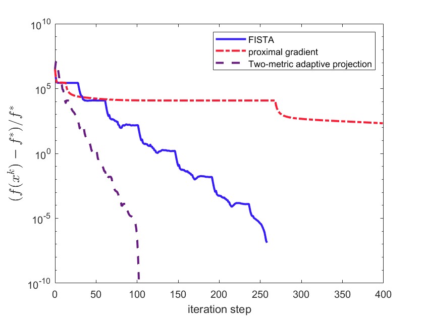
Figure 1: Comparison of methods on LASSO

The result shows that two-metric adaptive projection may have local superlinear convergence rate if we use Hessian, in sharp contrast with first-order methods such as FISTA [1] and proximal gradient [5].

7 Conclusion

In this article, we first define an approximate first-order optimal point for the bound-constrained problem. We investigate the iteration complexity of the two-metric projection method proposed by Bertsekas, the algorithm terminates within $\mathcal{O}(\epsilon^{-3})$ iterations and finds a point that is approximately first-order optimal to tolerance $\epsilon$. By scaling the diagonal matrix, we equip the method with a worst-case complexity theory that matches the best-known theoretical bounds for bound-constrained optimization and even unconstrained optimization. We also try to generalize the two-metric projection algorithm for composite optimization, we propose a framework called two-metric adaptive projection, which is suitable for solving the $\ell_{1}$-norm minimization problem.

In future work, we will consider the convergence properties of our two-metric adaptive projection and propose a general algorithm for composite optimization.

References

- [1] Amir Beck and Marc Teboulle. A fast iterative shrinkage-thresholding algorithm for linear inverse problems. SIAM Journal on Imaging Sciences, 2(1):183–202, 2009.
- [2] Dimitri P Bertsekas. Projected newton methods for optimization problems with simple constraints. SIAM Journal on Control and Optimization, 20(2):221–246, 1982.
- [3] Yair Carmon, John C Duchi, Oliver Hinder, and Aaron Sidford. Lower bounds for finding stationary points i. Mathematical Programming, 184(1-2):71–120, 2020.
- [4] Jorge Nocedal and Stephen J Wright. Numerical optimization. Springer, 1999.
- [5] Neal Parikh, Stephen Boyd, et al. Proximal algorithms. Foundations and trends® in Optimization, 1(3):127–239, 2014.