Decomposition-Invariant Pairwise Frank-Wolfe Algorithm for Constrained Multiobjective Optimization

Zhuoxin Fan zxfan42@gmail.com Liping Tang tanglps@163.com National Center for Applied Mathematics in Chongqing, Chongqing Normal University, Chongqing, 401331, China
Abstract

Recently the away-step Frank-Wolfe algoritm for constrained multiobjective optimization has been shown linear convergence rate over a polytope which is generated by finite points set. In this paper we design a decomposition-invariant pairwise frank-wolfe algorithm for multiobjective optimization that the feasible region is an arbitrary bounded polytope. We prove it has linear convergence rate of the whole sequence to a pareto optimal solution under strongly convexity without other assumptions.

keywords:
Multiobjective optimization , Frank-Wolfe method , Linear convergence rate , Decomposition-invariant
โ€ โ€ journal: Journal of ย Templates

1 Introduction

Constrained multiobjective optimization problem has casued much concern. Many problems in practical applications can be expressed as it, such as in engineering design[6], statics[3], machine learning[14].

Recently, The gradient-type method for solving the multiobjectvie optimization problem is popular. The first is steepest descent method[7] which is solving unconstrained multiobjectvie optimization problem. After that, projected gradient method[5], proximal point method[21] and conditional gradient method[1] have developed for solving constrained multiobjective optimization.

The conditional gradient method also named Frank-Wolfe method was first proposed by [8] for solving convex continuously differentiable optimization problems. And it has been extended to single-objective[18] and multiobjectvie optimization[1]. Frank-Wolfe method solves a linear optimization problem in each iteration, so it has advantages of simplicity and ease of implementation compared to projected gradient method. But the disadvantange of Frank-Wolfe method is obvious: its convergence rate is $\mathcal{O}(1/k)$ and can not be improved for general constrained convex optimization problems[13][16]. So many improvements to this disadvantange have been proposed such as pairwise, away-step Frank-Wolfe method[12][15] and conditional gradient sliding algorithm[17]. For constrained multiobjective optimization, [11] proposed the away-step Frank-Wolfe method. It attains linear convergence rate under certain assumptions. But the algorithm is to solve the problem that feasible region is a polytope generated by finite set of points. In this paper, we consider the feasible region is arbitrary polytopes. [2] and [10] have considered the single-objective optimization problems that these feasible regions are aribitary oplytopes. Combining with the ideas of them, we propose a new subproblem to calculate descent direction which we call pairwise direction. Under adaptive step size which is the natrual extension to multiobjective optimization, our algorithm also attain linear convergence rate when the objective functions have strongly convexity. Compared to the assumptions in away-step Frank-Wolfe algorithm for constrained multiobjective optimization, our assumptions do not need the additional assumption inequality (27) in [11] and is same as in [15].

The paper is organized as follows: Sect.2 introduces some notations, definitions and lemmas we will use. Sect.3 contains our main result: the decomposition-invariant pairwise Frank-Wolfe algorithm for multiobjective optimization. In Sect.4 we proved asymptotic convergence and the algorithm has linear convergence rate when objective functions are strongly convex. Sect.5 gives numberical experiments. Sect.6 contains the conclusion of this paper.

2 Preliminaries

This section, we give some notations and definitions. If not otherwise specified, the norm of this paper is Eulidean norm. Let $[n]$ denotes $\{1,2,...,n\}$, $[m]:=\{1,...,m\},R^{n}_{+}:=\{u\in R^{n}:u_{j}\geq 0,j\in[m]\}$, and $R^{n}_{++}:=\{u\in R^{n}:u_{j}>0,j\in[m]\}$. For $u,v\in R^{n},v\succeq u$ (or $u\preceq v$) means that $v-u\in R^{n}_{+}$ and $v\succ u$ (or $u\prec v$) means that $v-u\in R^{n}_{++}$. In general, a polytope $\mathcal{P}$ can be defined as

$$\mathcal{P}=\{x\in R^{n}:Ax\leq b,Cx=d\},$$

where $A=(a_{1},...,a_{m_{1}})^{\top}\in R^{m_{1}\times n}$, $b=(b_{1},...,b_{m_{1}})^{\top}\in R^{m_{1}}$, $C=(c_{1},...,c_{m_{2}})^{\top}\in R^{m_{2}\times n}$ and $d=(d_{1},...,d_{m_{2}})^{\top}\in R^{m_{2}}$. We denote the set of vertices of $\mathcal{P}$ is $\mathcal{V}$, the diameter of $\mathcal{P}$ is $D=\sup\{\|x-y\|:x,y\in\mathcal{P}\}$. In this paper we only concider $D<\infty$. We denote this constrained problem as

$\displaystyle\min$ $\displaystyle F(x)=(f_{1}(x),...,f_{m}(x))^{\top}$
s.t.formulae-sequence๐‘ ๐‘ก\displaystyle s.t. $\displaystyle Ax\leq b,$
$\displaystyle Cx=d.$

Throughout the paper we assume that $F:R^{n}\to R^{m}$ is a countinuously differentiable function given by $F:=(f_{1},...,f_{m})^{T}.$

Definition 2.1

A function $F:=(f_{1},...,f_{m})^{T}$ is Lโ€‹iโ€‹pโ€‹sโ€‹cโ€‹hโ€‹iโ€‹tโ€‹zโ€‹cโ€‹oโ€‹nโ€‹tโ€‹iโ€‹nโ€‹uโ€‹oโ€‹uโ€‹s๐ฟ๐‘–๐‘๐‘ ๐‘โ„Ž๐‘–๐‘ก๐‘ง๐‘๐‘œ๐‘›๐‘ก๐‘–๐‘›๐‘ข๐‘œ๐‘ข๐‘ Lipschitz\ continuous with respect to $||\cdot||$, if there exist constants $L_{1},...,L_{m}>0$ such that

$$f_{j}(y)\leq f_{j}(x)+\nabla f_{j}(x)\cdot(y-x)+\frac{L_{j}}{2}||x-y||^{2},\ \forall x,y\in\mathcal{C},\ \forall j\in[m].$$ (2)

For future reference we set $L:=\max\{L_{j}:j\in[m]\}.$

Definition 2.2

A function $F(x)=(f_{1}(x),...,f_{m}(x))^{\top}$ is convex over a convex set $\mathcal{C}\subset R^{n}$ if for all $j\in[m]$ it satisfies the following equivalent condtions

$\displaystyle f_{j}(y)\leq f_{j}(x)+\langle\nabla f_{j}(x),y-x\rangle\ \forall x,y\in\mathcal{C}.$ (3)

A point $x^{*}\in\mathcal{P}$ is called weak pareto optimal point for Problem (2), if there exists no other $x\in\mathcal{P}$ such that $F(x)\prec F(x^{*})$. $\mathcal{W}^{*}$ denotes the set of weak pareto potimal point for Problem (2). For a face $\mathcal{F}$ of $\mathcal{P}$, define $\dim\mathcal{F}$ as:

$$\dim\mathcal{F}:=n-\dim\mathtt{span}\{\{a_{1},...,a_{m_{1}}\}\cup\{c_{i}:1\leq i\leq m_{2},c_{i}^{\top}x=d_{i},\forall x\in\mathcal{F}\}\}.$$

Let $\mathcal{F}^{*}\subseteq\mathcal{P}$ is the lowest-dimensional face of $\mathcal{P}$ such that $\mathcal{W}^{*}\subseteq\mathcal{F}^{*}$. $\mathcal{F}^{*}$ can be written as $\mathcal{F}^{*}=\{x\in R^{n}:A^{*}x\leq b^{*},C^{*}x=d^{*}\}$. The rows of $A^{*}$ are the rows of $A$ that correspond to inequality constraints that are satisfied by some of the points in $\mathcal{F}^{*}$ but not by others, and $b^{*}$ is defined accordingly. The rows of $C^{*}$ are the rows of $C$ plus the rows of $A$ that correspond to inequality constraints that are tight for all points in $\mathcal{F}^{*}$ and $d^{*}$ is defiend accordingly. Denote $LI(\mathcal{P})$ the set of all $\dim\mathcal{F}^{*}\times n$ matrices whose rows are linearly independent rows chosen from the rows of $C^{*}$. We define

$$\phi^{*}=\max_{M\in LI(\mathcal{P})}\|M\|,\xi^{*}=\min_{v\in\mathcal{V}\cap\mathcal{F}^{*}}\min_{i}\{b(i)-A(i)^{\top}v|b(i)>A(i)^{\top}v\}.$$

$\phi^{*}$ and $\xi^{*}$ are constants for a polytope. For simplity, we define a useful function as

$$\sigma(x,z):=\min_{j\in[m]}[f_{j}(x)-f_{j}(z)].$$ (4)

3 Algorithms

The subproblem of classical frank-wolfe algorithm for multiobjective optimization[1] in the k-th iteration which we named FW-subproblem is

$$\min_{u\in\mathcal{P}}\max_{j\in[m]}\langle\nabla f_{j}(x^{k}),u-x^{k}\rangle.$$ (5)

We denote the optimal solution and value of it by $p^{FW}(x^{k})$ and $\theta^{FW}(x^{k})$, which means

$$p^{FW}(x^{k})\in\arg\min_{u\in\mathcal{P}}\max_{j\in[m]}\langle\nabla f_{j}(x^{k}),u-x^{k}\rangle,$$ (6)

and

$$\theta^{FW}(x^{k})=\min_{u\in\mathcal{P}}\max_{j\in[m]}\langle\nabla f_{j}(x^{k}),u-x^{k}\rangle.$$ (7)

The following lemma which is in [1] describle the property of $\theta^{FW}(x)$.

Lemma 3.1

For $\theta^{FW}(x)$, $x\in\mathcal{P}$, the following conclusions hold:

  • (i)

    $\theta^{FW}(x)\leq 0$;

  • (ii)

    $\theta^{FW}(x)$ is continous;

  • (iii)

    $\theta^{FW}(x^{*})=0$ if and only if $x^{*}\in\mathcal{P}$ is a weak Pareto optimal point of Problem (2).

The idea of away-step frank-wolfe algorithm [12][15] is to compute the classical diection and the away-step direction, then choose the better one. Our direction adopts the decompostion-invariant approach simillar with [2] and [10]. Our search space is restricted to the vertices that satisfy all the inequality constraints by equality if current $x^{k}$ does so:

$\displaystyle\min_{u,v\in R^{n}}\max_{j\in[m]}\langle\nabla f_{j}(x^{k}),u-v\rangle,$
s.t.formulae-sequence๐‘ ๐‘ก\displaystyle s.t. $\displaystyle Au\leq b,Cu=d$
$\displaystyle Av\leq b,Cv=d,\ and\ \langle a_{i},x^{k}\rangle=b_{i}\to\langle a_{i},u\rangle=b_{i},\forall i.$

The optimal value denotes $\theta^{PW}(x^{k})$, the optimal solution denotes $(p^{PW}(x^{k}),q^{PW}(x^{k}))$. This question is the has the following proposition. Its proof is the same as property 1 in [2]. In fact, property 1 in [2] is a special situation.

Proposition 3.1

Denote ๐’ฎโ€‹(x):={SโŠ‚๐’ซ:x=โˆ‘i=1tฮปiโ€‹si,siโˆˆSโ€‹aโ€‹nโ€‹dโ€‹ฮปi>0}assign๐’ฎ๐‘ฅconditional-set๐‘†๐’ซformulae-sequence๐‘ฅsubscriptsuperscript๐‘ก๐‘–1subscript๐œ†๐‘–subscript๐‘ ๐‘–subscript๐‘ ๐‘–๐‘†๐‘Ž๐‘›๐‘‘subscript๐œ†๐‘–0\mathcal{S}(x):=\{S\subset\mathcal{P}:x=\sum^{t}_{i=1}\lambda_{i}s_{i},s_{i}\in S\ and\ \lambda_{i}>0\}. Then (8) is equivalent to

minSโˆˆ๐’ฎโ€‹(x)โกminuโˆˆRn,vโˆˆSโกmaxjโˆˆ[m]โกโŸจโˆ‡fjโ€‹(x),uโˆ’vโŸฉโ€‹s.t.Aโ€‹uโ‰คb,Cโ€‹u=d.formulae-sequencesubscript๐‘†๐’ฎ๐‘ฅsubscriptformulae-sequence๐‘ขsuperscript๐‘…๐‘›๐‘ฃ๐‘†subscript๐‘—delimited-[]๐‘šโˆ‡subscript๐‘“๐‘—๐‘ฅ๐‘ข๐‘ฃ๐‘ ๐‘กformulae-sequence๐ด๐‘ข๐‘๐ถ๐‘ข๐‘‘\min_{S\in\mathcal{S}(x)}\min_{u\in R^{n},v\in S}\max_{j\in[m]}\langle\nabla f_{j}(x),u-v\rangle\ s.t.Au\leq b,Cu=d. (9)

We can get the relationship between $\theta^{PW}(x)$ and $\theta^{FW}(x)$ easily from Proposition (9).

Corollary 3.1

For any $x$ which is feasible, we have $\theta^{PW}(x)\leq\theta^{FW}(x)$.

Algorithm 1 Decomposition-Invariant Pisewise Frank-Wolfe Algorithm for Multiobjective Optimization
Initialization: $x_{1}\in\mathcal{P},\epsilon>0$.
forย k=1,2,โ€ฆ๐‘˜12โ€ฆk=1,2,...ย do
ย ย ย ย ย calculate pisewise direction $d^{PW}_{k}$ as ().
ย ย ย ย ย ifย โ€–ฮธFโ€‹Wโ€‹(xk)โ€–โ‰คฯตnormsuperscript๐œƒ๐น๐‘Šsuperscript๐‘ฅ๐‘˜italic-ฯต\|\theta^{FW}(x^{k})\|\leq\epsilonย then
ย ย ย ย ย ย ย ย ย Return $x^{k}$.
ย ย ย ย ย endย if
ย ย ย ย ย calculate $\lambda_{k,\max}$ such that $\lambda_{k,\max}=\max\{\lambda\geq 0:x^{k}+\lambda_{k}d^{PW}_{k}\in\mathcal{P}\}$.
ย ย ย ย ย Choose the step size $\lambda_{k}\in[0,\lambda_{k,\max}]$.
endย for

In Algorithm 1, the choice of step size is different from classical Frank-Wolfe algorithm. It is beacuse the algorithm should ensure that $x^{k+1}$ remains in the feasible region. No general solution is known to this difficulty. Our approach is doing line search or adaptive step size $\lambda_{k}=\min\{\lambda_{k,\max},\frac{-\theta^{PW}(x^{k})}{L\|d^{PW}(x^{k})\|}\}$.

Algorithm 2 Adaptive Step Size
Input:$F(x)$, $x\in\mathcal{C}$ and descent direction $d(x)$, smoothness parameter $L>0$,step size parameter $\lambda_{max}$ and progress parameters $\eta<1<\tau$.
$M=\eta L,\lambda=\min\{\lambda_{\max},\frac{-\max_{j\in[m]}\langle\nabla f_{j}(x),d(x)\rangle}{M\|d(x)\|^{2}}\}$.
whileย 
$$\{\max_{j\in[m]}(f_{j}(x+\lambda d(x))-f_{j}(x))\geq\lambda\max_{j\in[m]}\langle\nabla f_{j}(x),d(x)\rangle+\frac{\lambda^{2}M}{2}\|d(x)\|^{2}\}$$
ย do
ย ย ย ย ย M=ฯ„โ€‹M,ฮป=minโก{ฮปmax,โˆ’maxjโˆˆ[m]โกโŸจโˆ‡fjโ€‹(x),dโ€‹(x)โŸฉMโ€‹โ€–dโ€‹(x)โ€–2}formulae-sequence๐‘€๐œ๐‘€๐œ†subscript๐œ†subscript๐‘—delimited-[]๐‘šโˆ‡subscript๐‘“๐‘—๐‘ฅ๐‘‘๐‘ฅ๐‘€superscriptnorm๐‘‘๐‘ฅ2M=\tau M,\lambda=\min\{\lambda_{\max},\frac{-\max_{j\in[m]}\langle\nabla f_{j}(x),d(x)\rangle}{M\|d(x)\|^{2}}\}.
endย while
Ouput: updated smoothness parameter $L=M$ and step size $\lambda$.

Algorithm 2 is a generalized form of adaptive step size in [19]. We use

$$\max_{j\in[m]}(f_{j}(x+\lambda d(x))-f_{j}(x))\geq\lambda\max_{j\in[m]}\langle\nabla f_{j}(x),d(x)\rangle+\frac{\lambda^{2}M}{2}\|d(x)\|^{2}$$ (10)

instead of

$$\{(f_{j}(x+\lambda d(x))-f_{j}(x))\geq\lambda\langle\nabla f_{j}(x),d(x)\rangle+\frac{\lambda^{2}M}{2}\|d(x)\|^{2}\},\forall j\in[m].$$ (11)

Obviously, the first is weaker than the last inequality. And Algorithm 2 using either of these two ensures the following holds

$$\max_{j\in[m]}(f_{j}(x+\lambda d(x))-f_{j}(x))\leq\lambda\max_{j\in[m]}\langle\nabla f_{j}(x),d(x)\rangle+\frac{\lambda^{2}L}{2}\|d(x)\|^{2},$$

where $L,\lambda$ are output of Algorithm 2. Hence we choose the first inequality.

4 Convergence Analysis

In this section, we discuss the convergence analysis of Algorithm 1. Firstly, we discuss asymptotic convergence of Algorithm 1. Then we prove Algorithm 1 has $\mathcal{O}(1/k)$ for general constraint multiobjective convex optimization problem. However, if the objective function satisfies (13) which is weaker than strongly convexity, we can get linear convergence rate.

4.1 Asymptotic Convergence

We present the asymptotic convergence analysis of Algorithm 1 in this subsection. In Theorem 4.1, we have proved every limit point of $\{x^{k}:k\in\mathbb{N}\}$ generated by Algorithm 1 is a weak pareto point of Problem (2). If the objective function is strongly convex, every limit point of $\{x^{k}:k\in\mathbb{N}\}$ is a pareto point of Problem (2).

Lemma 4.1

Let $\{x^{k}:k\in\mathbb{N}\}$ be generated by Algorithm 1, we have

$$f_{j}(x^{k+1})\leq f_{j}(x^{k})+\lambda_{k}\theta^{PW}(x^{k})+\frac{L}{2}\lambda_{k}^{2}\|d^{PW}(x^{k})\|^{2},\forall j\in[m].$$ (12)

Proof. Since $F(x)=(f_{1}(x),...,f_{m}(x))^{\top}$ is Lipschitz continuous with $L$ on $\mathcal{P}$, we have

$\displaystyle f_{j}(x^{k+1})$ $\displaystyle\leq$ $\displaystyle f_{j}(x^{k})+\lambda_{k}\langle\nabla f_{j}(x^{k}),d^{PW}(x^{k})\rangle+\frac{L}{2}\lambda_{k}^{2}\|d^{PW}(x^{k})\|^{2}$
$\displaystyle\leq$ $\displaystyle f_{j}(x^{k})+\lambda_{k}\max_{j\in[m]}\langle\nabla f_{j}(x^{k}),d^{PW}(x^{k})\rangle+\frac{L}{2}\lambda_{k}^{2}\|d^{PW}(x^{k})\|^{2}$
$\displaystyle\leq$ $\displaystyle f_{j}(x^{k})+\lambda_{k}\theta^{PW}(x^{k})+\frac{L}{2}\lambda_{k}^{2}\|d^{PW}(x^{k})\|^{2}.$

$\square$

Remark 4.1

From the Lemma and the choice of step size $\lambda_{k}$, if none of the inequality constraints are satisfied as equality at the optimal $\lambda_{k}$ of line search, we call it a good step, otherwise we call it a bad step. For a bad step, we can only have that $f_{j}(x^{k+1})\leq f_{j}(x^{k}),\forall j\in[m]$. Fortunately we can bound the number of bad steps between two good steps.
First, if $\lambda_{k,\max}=1$ it is a good step. We know that if $d^{PW}(x^{k})=x^{k}$, $\lambda_{k,\max}=1$ holds. If $\lambda_{k,\max}<1$, at least one inequality constraint will turn into an equality constraint when doing line search. Algorithm 1 selects the search direction $d^{PW}(x^{k})$ by respecting all equality constraints, so succession of the search direction $d^{PW}(x^{k})$ will terminate when the set of equalities only define a singleton $x^{k}$. Since $x\in R^{n}$, it is obviously that the number of bad steps $bad(\mathcal{P})$ between two good steps is less than $n$.

Theorem 4.1

Every limit point of $\{x^{k}:k\in\mathbb{N}\}$ generated by Algorithm 1 is a weak Pareto optimal point of Problem (2).

Proof. From the Remark 4.1, we know there exists a subsequence of $\{x^{k}:k\in\mathbb{N}\}$ such that every in it is a good step. assume that the indices of subsequence is $K=\{k_{0},k_{1},...\}\subset\mathbb{N}$. Since $\mathcal{P}$ is compact and $x^{k}\in\mathcal{P}$ for all $k\in K$, we assume without loss of generality that $\{x^{k}:k\in K\}$ converge to $\bar{x}\in\mathcal{P}$. From the definition of $\theta^{FW}(x^{k})$ and $\theta^{PW}(x^{k})$, we have $\theta^{PW}(x^{k})\leq\theta^{FW}(x^{k})<0$, $\|d^{PW}(x^{k})\|\leq D$ where $D$ that is the diameter of $\mathcal{P}$. From Lemma , we have

$$f_{j}(x^{k_{i+1}})\leq f_{j}(x^{k_{i}})+\lambda_{k_{i}}\theta^{PW}(x^{k_{i}})+\frac{L}{2}\lambda_{k_{i}}^{2}\|d^{PW}(x^{k_{i}})\|^{2},\forall j\in[m],k_{i}\in K.$$

Since it is good step when $k_{i}\in K$, we have

$$f_{j}(x^{k_{i+1}})\leq f_{j}(x^{k_{i}})-\frac{\theta^{PW}(x^{k_{i}})^{2}}{2L\|d^{PW}(X^{k_{i}})\|^{2}},\forall j\in[m].$$

It follows that

$$\frac{\theta^{FW}(x^{k_{i}})^{2}}{2LD^{2}}\leq\frac{\theta^{PW}(x^{k_{i}})^{2}}{2LD^{2}}\leq f_{j}(x^{k_{i}})-f_{j}(x^{k_{i+1}}),\forall j\in[m].$$

But the sequence $\{F(x^{k}):k\in\mathbb{N}\}$ is monotonically decreaing, we have that the whole sequence $\{F(x^{k}):k\in\mathbb{N}\}$ converges to some point in $R^{m}$. It is because $\{x^{k}:k\in\mathbb{N}\}\subset\mathcal{P}$, $\mathcal{P}$ is compact and $F(x)$ is Lipschitz continuous. So we have that

$$\lim_{i\to\infty}\frac{\theta^{FW}(x^{k_{i}})^{2}}{2L\|d^{FW}(x^{k_{i}})\|^{2}}=0.$$

From Lemma 3.1, $\theta^{FW}(\bar{x})=0$ means that $\bar{x}$ is a weak Pareto optimal point for Problem (2). And $\{F(x^{k}):k\in\mathbb{N}\}$ converges to $F(\bar{x})$, hence any limit point $x^{*}\in\mathcal{P}$ of $\{x^{k}:k\in\mathbb{N}\}$ is a weak Pareto point for Problem (2). $\square$

Corollary 4.1

If $F(x)$ is $\mu$-strongly convex, then $\{x^{k}:k\in\mathbb{N}\}$ converges to a Pareto optimal point of Problem (2).

Proof. From Theorem 4.1, we know that a limit point $\bar{x}$ of $x^{*}\in\mathcal{P}$ is a weak Pareto point for Problem (2), it is also a critial point. So we have

$$\max_{j\in[m]}\langle\nabla f_{j}(\bar{x}),x^{k}-\bar{x}\rangle\geq 0,\forall j\in[m].$$

Since $F(x)$ is $\mu$-strongly convex, we have

$$f_{j}(x^{k})-f_{j}(\bar{x})\geq\langle\nabla f_{j}(\bar{x}),x^{k}-\bar{x}\rangle+\frac{\mu}{2}\|\bar{x}-x^{k}\|^{2},\forall j\in[m],k\in\mathbb{N}.$$

It follows that

$$\max_{j\in[m]}\{f_{j}(x^{k})-f_{j}(\bar{x})\}\geq\max_{j\in[m]}\langle\nabla f_{j}(\bar{x}),x^{k}-\bar{x}\rangle+\frac{\mu}{2}\|\bar{x}-x^{k}\|^{2}\geq\frac{\mu}{2}\|\bar{x}-x^{k}\|^{2}.$$

From the Theorem 4.1, we know that $F(x^{k})$ converges to a point that we conclude it as $F^{*}=(f_{1}^{*},...,f_{m}^{*})^{\top}$. Hence we have that $\{x^{k}:k\in\mathbb{N}\}$ converges to $\bar{x}$. Since $F(x)$ is strongly convex and $\bar{x}$ is weak Pareto point for Problem (2), it follows that $\bar{x}$ is a Pareto point for Problem (2). $\square$

4.2 Linear Convergence

We prove Algorithm 1 has $\mathcal{O}(1/k)$ when the objective function is general convex function. Lemma gives the upper bound of $\theta^{PW}(x^{k})$. Then we attains linear convergence rate when the objective function satisfies (13).

Assumption 4.1

Let $\{x^{k}:k\in\mathbb{N}\}$ generated by Algorithm 1 converges to a pareto optimal point $x^{*}$. There exists $\mu>0$ such that for all $j\in[m]$, $f_{j}(x)$ we have

$$\langle\nabla f_{j}(x^{k}),x^{*}-x^{k}\rangle\leq-\|x^{k}-x^{*}\|\sqrt{2\mu(f_{j}(x^{k})-f_{j}(x^{*}))},\forall j\in[m].$$ (13)
Remark 4.2

When $f_{j}(x),j\in[m]$ are strongly convex with $\mu_{j}>0$, (13) is satisfied with $\mu=\max\{\mu_{j},j\in[m]\}$.

The following lemma states any $y\in\mathcal{P}$ can be expressed as points of $\mathcal{V}$ and satisfies a useful proprety which is weaker than Lemma 5.3 of [9].

Lemma 4.2

Suppose $x$ can be written as some convex combination of s๐‘ s number of vertices of $\mathcal{P}$: x=โˆ‘i=1sฮปiโ€‹vi๐‘ฅsuperscriptsubscript๐‘–1๐‘ subscript๐œ†๐‘–subscript๐‘ฃ๐‘–x=\sum_{i=1}^{s}\lambda_{i}v_{i}, where ฮปiโ‰ฅ0,โˆ‘i=1sฮปi=1formulae-sequencesubscript๐œ†๐‘–0superscriptsubscript๐‘–1๐‘ subscript๐œ†๐‘–1\lambda_{i}\geq 0,\sum_{i=1}^{s}\lambda_{i}=1 and $v_{i}\in\mathcal{V}$. Then any $y\in\mathcal{P}$ can be written as y=โˆ‘i=1s(ฮปiโˆ’ฮ”i)โ€‹vi+ฮ”โ€‹z๐‘ฆsuperscriptsubscript๐‘–1๐‘ subscript๐œ†๐‘–subscriptฮ”๐‘–subscript๐‘ฃ๐‘–ฮ”๐‘งy=\sum_{i=1}^{s}(\lambda_{i}-\Delta_{i})v_{i}+\Delta z, such that $z\in\mathcal{P}$, ฮ”iโˆˆ[0,ฮปi],ฮ”=โˆ‘i=1sฮ”iformulae-sequencesubscriptฮ”๐‘–0subscript๐œ†๐‘–ฮ”superscriptsubscript๐‘–1๐‘ subscriptฮ”๐‘–\Delta_{i}\in[0,\lambda_{i}],\Delta=\sum_{i=1}^{s}\Delta_{i}. And for any iโˆˆ[s]๐‘–delimited-[]๐‘ i\in[s] such that $\Delta_{i}>0$, there exists at least an index jiโˆˆ[s1]subscript๐‘—๐‘–delimited-[]subscript๐‘ 1j_{i}\in[s_{1}] that satisfies $a_{j_{i}}^{\top}z=b_{j_{i}}$ and $a_{j_{i}}^{\top}v_{i}<b_{j_{i}}$.

Proof. Consider the following optimization problem:

minโกฮ”=โˆ‘i=1sฮ”iฮ”superscriptsubscript๐‘–1๐‘ subscriptฮ”๐‘–\displaystyle\min\Delta=\sum_{i=1}^{s}\Delta_{i}
s.t.formulae-sequence๐‘ ๐‘ก\displaystyle s.t. ฮ”iฮปi=ฮดโˆˆ[0,1],โˆ€iโˆˆ[s]formulae-sequencesubscriptฮ”๐‘–subscript๐œ†๐‘–๐›ฟ01for-all๐‘–delimited-[]๐‘ \displaystyle\ \frac{\Delta_{i}}{\lambda_{i}}=\delta\in[0,1],\forall i\in[s]
z=1ฮ”โ€‹(yโˆ’โˆ‘i=1s(ฮปiโˆ’ฮ”i)โ€‹vi)โˆˆ๐’ซ๐‘ง1ฮ”๐‘ฆsuperscriptsubscript๐‘–1๐‘ subscript๐œ†๐‘–subscriptฮ”๐‘–subscript๐‘ฃ๐‘–๐’ซ\displaystyle z=\frac{1}{\Delta}(y-\sum_{i=1}^{s}(\lambda_{i}-\Delta_{i})v_{i})\in\mathcal{P}
$\displaystyle\max_{j\in[m]}\langle\nabla f_{j}(x),q-x\rangle\leq\max_{j\in[m]}\langle\nabla f_{j}(x),y-x\rangle,$

where q=โˆ‘i=1s(ฮปiโˆ’ฮ”i)โ€‹vi+โˆ‘i=1sp๐‘žsuperscriptsubscript๐‘–1๐‘ subscript๐œ†๐‘–subscriptฮ”๐‘–subscript๐‘ฃ๐‘–superscriptsubscript๐‘–1๐‘ ๐‘q=\sum_{i=1}^{s}(\lambda_{i}-\Delta_{i})v_{i}+\sum_{i=1}^{s}p. Since when ฮ”i=ฮป,โˆ€iโˆˆ[s]formulae-sequencesubscriptฮ”๐‘–๐œ†for-all๐‘–delimited-[]๐‘ \Delta_{i}=\lambda,\forall i\in[s] we have $z=y$. It means that the feasible region of the problem is not empty and the optimal value of the problem is less than 1. Also $\Delta\geq 0$ means that the optimal value is nonnegative. There exists iโˆˆ[s]๐‘–delimited-[]๐‘ i\in[s] such that $\Delta_{i}>0$, and an index jiโˆˆ[s1]subscript๐‘—๐‘–delimited-[]subscript๐‘ 1j_{i}\in[s_{1}] that satisfies $a_{j_{i}}^{\top}z=b_{j_{i}}$ and $a_{j_{i}}^{\top}v_{i}<b_{j_{i}}$. Otherwise we can find $\Delta_{i}^{\prime}<\Delta_{i}$ and satisfies conditions. $\square$

Lemma 4.3

Let $x\in\mathcal{P}$ and write $x$ as a convex combination of points in $\mathcal{P}$,i.e., x=โˆ‘i=1sฮปiโ€‹vi๐‘ฅsuperscriptsubscript๐‘–1๐‘ subscript๐œ†๐‘–subscript๐‘ฃ๐‘–x=\sum_{i=1}^{s}\lambda_{i}v_{i} such that $\lambda_{i}>0$ for all i=1,โ€ฆ,s๐‘–1โ€ฆ๐‘ i=1,...,s. Let $y\in\mathcal{P}$. $y$ can be written as a convex combination y=โˆ‘i=1s(ฮปiโˆ’ฮ”i)โ€‹vi+โˆ‘i=1sฮ”iโ€‹z๐‘ฆsuperscriptsubscript๐‘–1๐‘ subscript๐œ†๐‘–subscriptฮ”๐‘–subscript๐‘ฃ๐‘–superscriptsubscript๐‘–1๐‘ subscriptฮ”๐‘–๐‘งy=\sum_{i=1}^{s}(\lambda_{i}-\Delta_{i})v_{i}+\sum_{i=1}^{s}\Delta_{i}z for some $z\in\mathcal{P},\Delta_{i}\in[0,\lambda_{i}]$. Let ฮ”=โˆ‘i=1sฮ”iฮ”superscriptsubscript๐‘–1๐‘ subscriptฮ”๐‘–\Delta=\sum_{i=1}^{s}\Delta_{i} is minimized. We have

โˆ‘i=1sฮ”iโ‰คm1โ€‹ฯ•โˆ—ฮพโˆ—โ€‹โ€–yโˆ’xโ€–.superscriptsubscript๐‘–1๐‘ subscriptฮ”๐‘–subscript๐‘š1superscriptitalic-ฯ•superscript๐œ‰norm๐‘ฆ๐‘ฅ\sum_{i=1}^{s}\Delta_{i}\leq\frac{m_{1}\phi^{*}}{\xi^{*}}\|y-x\|. (14)

Proof. From Lemma 4.2, we know that exists iโˆˆ[s]๐‘–delimited-[]๐‘ i\in[s] and $j_{i}$ such that $a_{j_{i}}^{\top}z=b_{j_{i}}$ and $a_{j_{i}}^{\top}v_{i}<b_{j_{i}}$. Let $C^{*}(z)\subset[m_{1}]$ be a set of minimal cardinality such that i) for all $j\in C^{*}(z)$, $a_{j}^{\top}z=b_{j}$, ii) for all iโˆˆ[s]๐‘–delimited-[]๐‘ i\in[s] there exists $j_{i}\in C^{*}(z)$ for which $a_{j_{i}}^{\top}v_{i}<b_{j_{i}}$. Let $A_{z}\in R^{|C^{*}(z)|\times n}$ be the matrix $A$ that deletes each row $j\notin C^{*}(z)$. We have that

$\displaystyle\|y-x\|^{2}\geq$ $\displaystyle\frac{1}{\|A_{z}\|^{2}}\|A_{z}(y-x)\|^{2}$
$\displaystyle=$ 1โ€–Azโ€–2โ€‹โ€–Azโ€‹โˆ‘i=1sฮ”iโ€‹(zโˆ’vi)โ€–21superscriptnormsubscript๐ด๐‘ง2superscriptnormsubscript๐ด๐‘งsuperscriptsubscript๐‘–1๐‘ subscriptฮ”๐‘–๐‘งsubscript๐‘ฃ๐‘–2\displaystyle\frac{1}{\|A_{z}\|^{2}}\|A_{z}\sum_{i=1}^{s}\Delta_{i}(z-v_{i})\|^{2}
$\displaystyle\geq$ 1ฯ•โˆ—2โ€‹โˆ‘jโˆˆCโˆ—โ€‹(z)(โˆ‘i=1sฮ”iโ€‹(bjโˆ’ajโŠคโ€‹vi))21superscriptitalic-ฯ•absent2subscript๐‘—superscript๐ถ๐‘งsuperscriptsuperscriptsubscript๐‘–1๐‘ subscriptฮ”๐‘–subscript๐‘๐‘—superscriptsubscript๐‘Ž๐‘—topsubscript๐‘ฃ๐‘–2\displaystyle\frac{1}{\phi^{*2}}\sum_{j\in C^{*}(z)}(\sum_{i=1}^{s}\Delta_{i}(b_{j}-a_{j}^{\top}v_{i}))^{2}
$\displaystyle\geq$ 1ฯ•โˆ—2โ€‹|Cโˆ—โ€‹(z)|โ€‹(โˆ‘jโˆˆCโˆ—โ€‹(z)โˆ‘i=1sฮ”iโ€‹(bjโˆ’ajโŠคโ€‹vi))21superscriptitalic-ฯ•absent2superscript๐ถ๐‘งsuperscriptsubscript๐‘—superscript๐ถ๐‘งsuperscriptsubscript๐‘–1๐‘ subscriptฮ”๐‘–subscript๐‘๐‘—superscriptsubscript๐‘Ž๐‘—topsubscript๐‘ฃ๐‘–2\displaystyle\frac{1}{\phi^{*2}|C^{*}(z)|}(\sum_{j\in C^{*}(z)}\sum_{i=1}^{s}\Delta_{i}(b_{j}-a_{j}^{\top}v_{i}))^{2}
$\displaystyle\geq$ 1ฯ•โˆ—2โ€‹|Cโˆ—โ€‹(z)|โ€‹(โˆ‘i=1sฮ”iโ€‹ฮพโˆ—)21superscriptitalic-ฯ•absent2superscript๐ถ๐‘งsuperscriptsuperscriptsubscript๐‘–1๐‘ subscriptฮ”๐‘–superscript๐œ‰2\displaystyle\frac{1}{\phi^{*2}|C^{*}(z)|}(\sum_{i=1}^{s}\Delta_{i}\xi^{*})^{2}
$\displaystyle\geq$ ฮพโˆ—2m1โ€‹ฯ•โˆ—2โ€‹(โˆ‘i=1sฮ”i)2.superscript๐œ‰absent2subscript๐‘š1superscriptitalic-ฯ•absent2superscriptsuperscriptsubscript๐‘–1๐‘ subscriptฮ”๐‘–2\displaystyle\frac{\xi^{*2}}{m_{1}\phi^{*2}}(\sum_{i=1}^{s}\Delta_{i})^{2}.

Hence we have

โˆ‘i=1sฮ”iโ‰คm1โ€‹ฯ•โˆ—ฮพโˆ—โ€‹โ€–yโˆ’xโ€–.superscriptsubscript๐‘–1๐‘ subscriptฮ”๐‘–subscript๐‘š1superscriptitalic-ฯ•superscript๐œ‰norm๐‘ฆ๐‘ฅ\sum_{i=1}^{s}\Delta_{i}\leq\frac{m_{1}\phi^{*}}{\xi^{*}}\|y-x\|.

$\square$

Lemma 4.4

Let $\{x^{k},k\in\mathbb{N}\}$ is generated by Algorithm 1. Let $(p^{PW}(x^{k}),q^{PW}(x^{k}))$ is the optimal solution of Problem (2) at $x^{k}$. Then for any $y\in\mathcal{P}$ we have

$\displaystyle\frac{\max_{j\in[m]}\langle\nabla f_{j}(x^{k}),y-x^{k}\rangle}{\|y-x^{k}\|}$ $\displaystyle\geq$ $\displaystyle\frac{m_{1}\phi^{*}}{\xi^{*}}\max_{j\in[m]}\langle\nabla f_{j}(x^{k}),p^{PW}(x^{k})-q^{PW}(x^{k})\rangle$ (15)
$\displaystyle=$ $\displaystyle\frac{m_{1}\phi^{*}}{\xi^{*}}\theta^{PW}(x^{k}).$

Proof. $x^{k}$ can write the convex decomposition as xk=โˆ‘i=1sฮปiโ€‹vi,{vi,iโˆˆ[s]}โŠ‚๐’ฑformulae-sequencesuperscript๐‘ฅ๐‘˜superscriptsubscript๐‘–1๐‘ subscript๐œ†๐‘–subscript๐‘ฃ๐‘–subscript๐‘ฃ๐‘–๐‘–delimited-[]๐‘ ๐’ฑx^{k}=\sum_{i=1}^{s}\lambda_{i}v_{i},\{v_{i},i\in[s]\}\subset\mathcal{V}. Let ฮ”k=โˆ‘i=1sฮ”isuperscriptฮ”๐‘˜superscriptsubscript๐‘–1๐‘ subscriptฮ”๐‘–\Delta^{k}=\sum_{i=1}^{s}\Delta_{i}. From Lemma 4.3, we know that y=โˆ‘i=1s(ฮปiโˆ’ฮ”i)โ€‹vi+ฮ”kโ€‹z๐‘ฆsuperscriptsubscript๐‘–1๐‘ subscript๐œ†๐‘–subscriptฮ”๐‘–subscript๐‘ฃ๐‘–superscriptฮ”๐‘˜๐‘งy=\sum_{i=1}^{s}(\lambda_{i}-\Delta_{i})v_{i}+\Delta^{k}z, where $z\in\mathcal{P}$, and โˆ‘i=1sฮ”iโ‰คm1โ€‹ฯ•โˆ—ฮพโˆ—โ€‹โ€–yโˆ’xkโ€–superscriptsubscript๐‘–1๐‘ subscriptฮ”๐‘–subscript๐‘š1superscriptitalic-ฯ•superscript๐œ‰norm๐‘ฆsuperscript๐‘ฅ๐‘˜\sum_{i=1}^{s}\Delta_{i}\leq\frac{m_{1}\phi^{*}}{\xi^{*}}\|y-x^{k}\|. Let xฮ”k=1ฮ”kโ€‹โˆ‘i=1sฮ”iโ€‹viโˆˆ๐’ซsuperscript๐‘ฅsuperscriptฮ”๐‘˜1superscriptฮ”๐‘˜superscriptsubscript๐‘–1๐‘ subscriptฮ”๐‘–subscript๐‘ฃ๐‘–๐’ซx^{\Delta^{k}}=\frac{1}{\Delta^{k}}\sum_{i=1}^{s}\Delta_{i}v_{i}\in\mathcal{P}. Concider

tk=โˆ‘i=1s(ฮปiโˆ’ฮ”i)โ€‹vi+ฮ”kโ€‹pโ€‹(xk,xฮ”k),superscript๐‘ก๐‘˜superscriptsubscript๐‘–1๐‘ subscript๐œ†๐‘–subscriptฮ”๐‘–subscript๐‘ฃ๐‘–superscriptฮ”๐‘˜๐‘superscript๐‘ฅ๐‘˜superscript๐‘ฅsuperscriptฮ”๐‘˜t^{k}=\sum_{i=1}^{s}(\lambda_{i}-\Delta_{i})v_{i}+\Delta^{k}p(x^{k},x^{\Delta^{k}}),

where $p(x^{k},x^{\Delta^{k}})$ is the optimal solution of the following question:

$$\min_{u\in\mathcal{P}}\max_{j\in[m]}\langle\nabla f_{j}(x^{k}),u-x^{\Delta^{k}}\rangle.$$

Since $p(x^{k},x^{\Delta^{k}})-x^{\Delta^{k}}=\frac{1}{\Delta^{k}}(t^{k}-x^{k})$ and $z-x^{\Delta^{k}}=\frac{1}{\Delta^{k}}(y-x^{k})$, we have

$\displaystyle\frac{1}{\Delta^{k}}\max_{j\in[m]}\langle\nabla f_{j}(x^{k}),t^{k}-x^{k}\rangle$ $\displaystyle=$ $\displaystyle\max_{j\in[m]}\langle\nabla f_{j}(x^{k}),p(x^{k},x^{\Delta^{k}})-x^{\Delta^{k}}\rangle$
$\displaystyle\leq$ $\displaystyle\max_{j\in[m]}\langle\nabla f_{j}(x^{k}),z-x^{\Delta^{k}}\rangle$
$\displaystyle=$ $\displaystyle\frac{1}{\Delta^{k}}\max_{j\in[m]}\langle\nabla f_{j}(x^{k}),y-x^{k}\rangle.$

From $\Delta^{k}>0$ we have that $\max_{j\in[m]}\langle\nabla f_{j}(x^{k}),t^{k}-x^{k}\rangle\geq\max_{j\in[m]}\langle\nabla f_{j}(x^{k}),y-x^{k}\rangle$. Now we can establish the relationship between $y$ and $(p^{PW}(x^{k}),q^{PW}(x^{k}))$.

$\displaystyle\max_{j\in[m]}\langle\nabla f_{j}(x^{k}),y-x^{k}\rangle$ $\displaystyle\geq$ $\displaystyle\max_{j\in[m]}\langle\nabla f_{j}(x^{k}),t^{k}-x^{k}\rangle$
$\displaystyle=$ maxjโˆˆ[m]โกโŸจโˆ‡fjโ€‹(xk),ฮ”kโ€‹pโ€‹(xk,xฮ”k)โˆ’โˆ‘i=1sฮ”iโ€‹viโŸฉsubscript๐‘—delimited-[]๐‘šโˆ‡subscript๐‘“๐‘—superscript๐‘ฅ๐‘˜superscriptฮ”๐‘˜๐‘superscript๐‘ฅ๐‘˜superscript๐‘ฅsuperscriptฮ”๐‘˜superscriptsubscript๐‘–1๐‘ subscriptฮ”๐‘–subscript๐‘ฃ๐‘–\displaystyle\max_{j\in[m]}\langle\nabla f_{j}(x^{k}),\Delta^{k}p(x^{k},x^{\Delta^{k}})-\sum_{i=1}^{s}\Delta_{i}v_{i}\rangle
$\displaystyle=$ ฮ”kโ€‹maxjโˆˆ[m]โกโŸจโˆ‡fjโ€‹(xk),pโ€‹(xk,xฮ”k)โˆ’1ฮ”kโ€‹โˆ‘i=1sฮ”iโ€‹viโŸฉsuperscriptฮ”๐‘˜subscript๐‘—delimited-[]๐‘šโˆ‡subscript๐‘“๐‘—superscript๐‘ฅ๐‘˜๐‘superscript๐‘ฅ๐‘˜superscript๐‘ฅsuperscriptฮ”๐‘˜1superscriptฮ”๐‘˜superscriptsubscript๐‘–1๐‘ subscriptฮ”๐‘–subscript๐‘ฃ๐‘–\displaystyle\Delta^{k}\max_{j\in[m]}\langle\nabla f_{j}(x^{k}),p(x^{k},x^{\Delta^{k}})-\frac{1}{\Delta^{k}}\sum_{i=1}^{s}\Delta_{i}v_{i}\rangle
$\displaystyle\geq$ $\displaystyle\Delta^{k}\max_{j\in[m]}\langle\nabla f_{j}(x^{k}),p^{PW}(x^{k})-q^{PW}(x^{k})\rangle=\Delta^{k}\theta^{PW}(x^{k}).$

Combining the inequality and Lemma 4.3, we get the conclusion. $\square$

Remark 4.3

Let $y=x^{*}$ which is a limit point of $\{x^{k}:k\in\mathbb{N}\}$ generated by Algorithm 1, and from Lemma 4.4 we build the relation between $\theta^{PW}(x^{k})$ and $\max_{j\in[m]}\langle\nabla f_{j}(x^{k}),x^{*}-x^{k}\rangle$. Acturally the coefficient $\frac{m_{1}\phi^{*}}{\xi^{*}}$ of $\theta^{PW}(x^{k})$ is a constant with respect to $\mathcal{P}$. When $m=1$ this result degraded to the single-objective optimization. Then the facial distance in [20] or the pyramidal width in [15] can be applied to replace.

Theorem 4.2

Let $\{x^{k}:k\in\mathbb{N}\}$ be generated by Algorithm 1 and $x^{*}$ is a limit point. Denote $\sigma(x^{k},x^{*})=\min_{j\in[m]}\{f_{j}(x^{k})-f_{j}(x^{*})\}$. Then we have

$$\sigma(x^{k},x^{*})=\mathcal{O}(\beta D^{2}/k),\forall k\geq 1.$$ (16)

Assume that $F(x)$ satisfies (13), we have

$$\sigma(x^{k+1},x^{*})\leq(1-\frac{2\mu\xi^{*2}}{2LD^{2}m_{1}^{2}\phi^{*2}})\sigma(x^{k},x^{*}).$$ (17)

Proof. Comining the proof of Theorem 4.1 and Remark 4.1, (16) is obtained immediately. Now we prove (17) holds if (13) is satisfied.
First, we concider a good step. From (13) of $F(x)$ and Lemma 4.4 we have that

$\displaystyle\theta^{PW}(x^{k})$ $\displaystyle\leq$ $\displaystyle\frac{\xi^{*}}{m_{1}\phi^{*}\|x^{*}-x^{k}\|}\max_{j\in[m]}\langle\nabla f_{j}(x^{k}),x^{*}-x^{k}\rangle$
$\displaystyle\leq$ $\displaystyle-\frac{\sqrt{2\mu}\xi^{*}}{m_{1}\phi^{*}}\sqrt{\sigma(x^{k},x^{*})}.$

For a good step, the step size $\lambda_{k}=-\frac{\theta^{PW}(x^{k})}{L\|d^{PW}(x^{k})\|^{2}}<\lambda_{k,max}$. Accroding the smoothess of $F(x)$ we have that

$\displaystyle f_{j}(x^{k+1})$ $\displaystyle\leq$ $\displaystyle f_{j}(x^{k})-\lambda_{k}\langle\nabla f_{j}(x^{k}),d^{PW}(x^{k})\rangle+\frac{L}{2}\lambda_{k}^{2}\|d^{PW}(x^{k})\|^{2}$
$\displaystyle\leq$ $\displaystyle f_{j}(x^{k})-\lambda_{k}\theta^{PW}(x^{k})+\frac{L}{2}\lambda_{k}^{2}\|d^{PW}(x^{k})\|^{2}.$

Hence we have that

$\displaystyle\sigma(x^{k+1},x^{*})$ $\displaystyle\leq$ $\displaystyle\sigma(x^{k},x^{*})-\lambda_{k}\theta^{PW}(x^{k})+\frac{L}{2}\lambda_{k}^{2}\|d^{PW}(x^{k})\|^{2}$
$\displaystyle=$ $\displaystyle\sigma(x^{k},x^{*})-\frac{\theta^{PW}(x^{k})^{2}}{2L\|d^{PW}(x^{k})\|^{2}}\leq\sigma(x^{k},x^{*})-\frac{2\mu\xi^{*2}}{2LD^{2}m_{1}^{2}\phi^{*2}}\sigma(x^{k},x^{*}).$

We get the conclusion. $\square$

5 Numberical Experiments

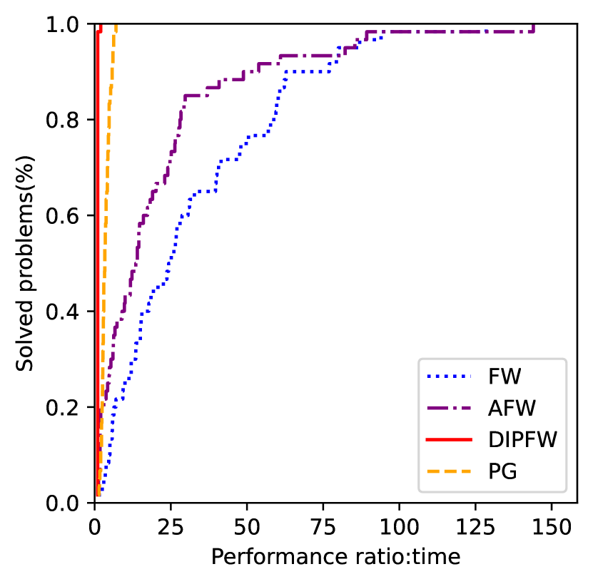
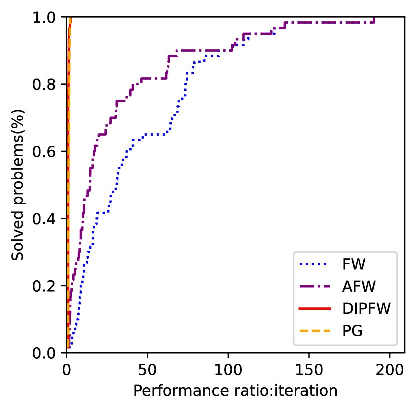
This section we present some numberical experiments illustrating the good performance of DIPFWMOP. As a contrast, We consider Frank-Wolfe algorithm for multiobjective optimization[1], Away-step Frank-Wolfe algorithm for multiobjective optimization[11] and Projected Gradient method for multiobjective optimization[5]. For simplicity, we call them as FW, AFW, DIPFW and PG in the follows. All of numberical experiments are implemented in PYTHON.

We have described the subproblem and the adaptive step size for FW, AFW and DIPFW in sect.3. It should be noted that adaptive step size may fail when accuracy is required. Hence the smoothness parameter each cycle is multiplied by a parameter $\alpha=0.5$. Now we will briefly describe PG. The subproblem of PG at each iteration is

$\displaystyle\min_{u\in\mathcal{P}}\max_{j\in[m]}\langle\nabla f_{j}(x^{k}),u-x^{k}\rangle+\frac{1}{2}\|u-x^{k}\|^{2}.$ (18)

It is a quadratic problem, so we use cvxpy to solve it. The stopping criterion we use is $\frac{1}{2}\|p(x^{k})-x^{k}\|^{2}<\epsilon$ where $p(x^{k})$ is the solution of subproblem of PG and $\epsilon>0$ is the tolerance. The step size we choose is the armijo line search. We consider the following multiobjective optimization problem

$\displaystyle\min_{x\in\mathbb{R}^{n}}$ $\displaystyle F(x)=(\frac{1}{2}\|y-b_{1}\|^{2},...,\frac{1}{2}\|y-b_{m}\|^{2})^{\top},$
s.t.formulae-sequence๐‘ ๐‘ก\displaystyle s.t. $\displaystyle\ y=Ax,$
$\displaystyle x\geq 0,e^{\top}x=1,$

where $e=(1,1,...,1)^{\top}\in R^{m}$, $A=(a_{1},...,a_{n})\in R^{p\times n}$, and $b_{j}\in R^{p},j\in[m]$. $a_{i}$ of $A$ and $b_{j},j\in[m]$ are selected ramdomly in $[0,1]^{p}$. We let $p=10,20,50$, $n=10$ and $m=2,3$. The tolerance $\epsilon$ is $10^{-4}$.

Tab.1 lists the time and iteration result which four algorithms have run. From Fig.1, we know that DIPFW and PG is better than FW and AFW in most text problems. And DIPFW is faster than PG in time.

In Fig.1, we plot four algorithmsโ€™ performance profile for time and iteration which is proposed in [4]. Fig.1 similarly illustrates DIPFW is better than others.

time iteration
Method Dim Min Mean Max Min Mean Max
FW (10,10,2) 3.172 4.697 7.343 1457 2082.3 2923
AFW (10,10,2) 3.234 4.784 6.672 1419 2074.9 2846
DIPFW (10,10,2) 0.078 1.109 0.141 22 35.2 48
PG (10,10,2) 0.156 0.220 0.281 21 27.8 37
FW (10,10,3) 0.031 1.288 2.047 9 343 549
AFW (10,10,3) 0.031 0.816 1.312 8 229.9 338
DIPFW (10,10,3) 0.031 0.053 0.063 10 17.5 22
PG (10,10,3) 0.094 0.159 0.281 13 19.1 32
FW (10,20,2) 3.563 3.713 3.891 1715 1763.7 1797
AFW (10,20,2) 0.078 0.097 0.125 38 44.8 59
DIPFW (10,20,2) 0.047 0.061 0.078 17 22.6 27
PG (10,20,2) 0.203 0.278 0.328 22 33.2 39
FW (10,20,3) 0.156 0.530 1.344 60 235.2 596
AFW (10,20,3) 0.125 0.541 1.375 59 230.3 582
DIPFW (10,20,3) 0.047 0.053 0.063 15 18.8 23
PG (10,20,3) 0.125 0.161 0.188 16 19.2 23
FW (10,50,2) 0.469 3.958 16.063 208 1775.5 7228
AFW (10,50,2) 0.5 4.233 18 207 1774.5 7227
DIPFW (10,50,2) 0.094 0.114 0.141 27 33.9 41
PG (10,50,2) 0.281 0.327 0.406 36 41.3 51
FW (10,50,3) 0.219 0.653 0.969 96 274.7 418
AFW (10,50,3) 0.234 0.673 1 95 273.7 417
DIPFW (10,50,3) 0.063 0.066 0.781 21 24.2 28
PG (10,50,3) 0.297 0.353 0.391 39 42.6 46
Table 1: time and iteration
Refer to caption
(a) time
Refer to caption
(b) iteration
Figure 1: time(left) and iteration(right).

6 Conclusion

In this paper, we propose decomposition-invariant pairwise Frank-Wolfe algorithm for constrained multiobjective optimization. This algorithm solve constrained multiobjective optimization problems whose feasible region is an arbitrary bounded polytope. The descent direction of the algorithm combines pairwise direction. We establish asymptotic convergence analysis and linear convergence rate if objective functions are strongly convex.

In future work, we will extend this algorithm to the vector optimization and analysis its convergence.

References

  • [1] PBย Assunรงรฃo, Orizonย Pereira Ferreira, and LFย Prudente. Conditional gradient method for multiobjective optimization. Computational Optimization and Applications, 78:741โ€“768, 2021.
  • [2] Mohammadย Ali Bashiri and Xinhua Zhang. Decomposition-invariant conditional gradient for general polytopes with line search. Advances in neural information processing systems, 30, 2017.
  • [3] Emilio Carrizosa and Johannes Bartholomeusย Gerardus Frenk. Dominating sets for convex functions with some applications. Journal of Optimization Theory and Applications, 96:281โ€“295, 1998.
  • [4] Elizabethย D Dolan and Jorgeย J Morรฉ. Benchmarking optimization software with performance profiles. Mathematical programming, 91:201โ€“213, 2002.
  • [5] LMย Grana Drummond and Alfredoย N Iusem. A projected gradient method for vector optimization problems. Computational Optimization and applications, 28:5โ€“29, 2004.
  • [6] Hans Eschenauer, Juhani Koski, and Andrzej Osyczka. Multicriteria design optimization: procedures and applications. Springer Science & Business Media, 2012.
  • [7] Jรถrg Fliege and Benarย Fux Svaiter. Steepest descent methods for multicriteria optimization. Mathematical methods of operations research, 51:479โ€“494, 2000.
  • [8] Marguerite Frank, Philip Wolfe, etย al. An algorithm for quadratic programming. Naval research logistics quarterly, 3(1-2):95โ€“110, 1956.
  • [9] Dan Garber and Elad Hazan. A linearly convergent variant of the conditional gradient algorithm under strong convexity, with applications to online and stochastic optimization. SIAM Journal on Optimization, 26(3):1493โ€“1528, 2016.
  • [10] Dan Garber and Ofer Meshi. Linear-memory and decomposition-invariant linearly convergent conditional gradient algorithm for structured polytopes. Advances in neural information processing systems, 29, 2016.
  • [11] Douglasย S Gonรงalves, Maxย LN Gonรงalves, and Jeffersonย G Melo. An away-step frankโ€“wolfe algorithm for constrained multiobjective optimization. Computational Optimization and Applications, pages 1โ€“23, 2024.
  • [12] Jacques Guรฉlat and Patrice Marcotte. Some comments on wolfeโ€™s โ€˜away stepโ€™. Mathematical Programming, 35(1):110โ€“119, 1986.
  • [13] Martin Jaggi. Revisiting frank-wolfe: Projection-free sparse convex optimization. In International conference on machine learning, pages 427โ€“435. PMLR, 2013.
  • [14] Yaochu Jin. Multi-objective machine learning, volumeย 16. Springer Science & Business Media, 2007.
  • [15] Simon Lacoste-Julien and Martin Jaggi. On the global linear convergence of frank-wolfe optimization variants. Advances in neural information processing systems, 28, 2015.
  • [16] Guanghui Lan. The complexity of large-scale convex programming under a linear optimization oracle. arXiv preprint arXiv:1309.5550, 2013.
  • [17] Guanghui Lan and Yiย Zhou. Conditional gradient sliding for convex optimization. SIAM Journal on Optimization, 26(2):1379โ€“1409, 2016.
  • [18] Evgenyย S Levitin and Borisย T Polyak. Constrained minimization methods. USSR Computational mathematics and mathematical physics, 6(5):1โ€“50, 1966.
  • [19] Fabian Pedregosa, Geoffrey Negiar, Armin Askari, and Martin Jaggi. Linearly convergent frank-wolfe with backtracking line-search. In International conference on artificial intelligence and statistics, pages 1โ€“10. PMLR, 2020.
  • [20] Javier Pena and Daniel Rodriguez. Polytope conditioning and linear convergence of the frankโ€“wolfe algorithm. Mathematics of Operations Research, 44(1):1โ€“18, 2019.
  • [21] Hiroki Tanabe, Ellenย H Fukuda, and Nobuo Yamashita. Proximal gradient methods for multiobjective optimization and their applications. Computational Optimization and Applications, 72:339โ€“361, 2019.