On pattern formation in the thermodynamically-consistent variational Gray-Scott model

Abstract

In this paper, we explore pattern formation in a four-species variational Gary-Scott model, which includes all reverse reactions and introduces a virtual species to describe the birth-death process in the classical Gray-Scott model. This modification transforms the classical Gray-Scott model into a thermodynamically consistent closed system. The classical two-species Gray-Scott model can be viewed as a subsystem of the variational Gray-Scott model in the limiting case when the small parameter $\epsilon$, related to the reaction rate of the reverse reactions, approaches zero. We numerically study the physically more complete Gray-Scott model with various $\epsilon$ in one dimension. By decreasing $\epsilon$, we observed that the stationary pattern in the classical Gray-Scott model can be stabilized as the transient state in the variational model for a significantly small $\epsilon$. Additionally, the variational model admits oscillated and traveling-wave-like pattern for small $\epsilon$. The persistent time of these patterns is on the order of $\mathcal{O}(\epsilon^{-1})$. We also analyze the stability of two uniform steady states in the variational Gary-Scott model for fixed $\epsilon$. Although both states are stable in a certain sense, the gradient flow type dynamics of the variational model exhibit a selection effect based on the initial conditions, with pattern formation occurring only if the initial condition does not converge to the boundary steady state, which corresponds to the trivial uniform steady state in the classical Gray-Scott model.

1 Introduction

Pattern formation is an emerging phenomenon observed across various disciplines including biology, chemistry, physics, and engineering. Examples of pattern formation range from the stripes of a zebra to the spirals of a galaxy [1]. Understanding mechanisms and principles behind pattern formation has been a longstanding scientific question. Mathematical models play a crucial role in understanding pattern formation, offering a powerful tool to unravel its intricate dynamics, uncover fundamental principles, and predict complex behaviors [2, 3, 4]. During past decades, significant contributions have advanced our understanding of pattern formation, including the molecular underpinnings [5], modeling dispersal in biological systems [6], investigating dynamic pattern formation in cellular networks [7], and exploring multiscale models of developmental systems [8]. Reaction-diffusion equations, rooted in the seminal work of Alan Turing [3], have been one of the best-known mathematical models used to explain pattern formation [9]. Arising from Turing instability, reaction-diffusion models can generate a wide variety of spatial patterns. These models find applications in diverse fields, such as biology, where they are used to model processes like morphogenesis and tissue patterning [10, 11]; chemistry, for understanding reaction-diffusion dynamics [12, 13]; and physics, for exploring phenomena like convection and fracture patterns [14]. Recent advances in the mathematical studying of pattern formation include the integration of computational techniques to compute multiple patterns [15, 16, 17, 18, 19, 20], as well as the application of machine learning methods to analyze complex pattern formation from data and discover novel patterns [21, 18].

One of the most well-known reaction-diffusion systems for pattern formation is the Gray-Scott model, which can generate a diverse range of spatial patterns [22, 23, 24, 25]. Originally proposed by Gray and Scott [26, 27], this model consists of two reacting chemical species in a system of two ordinary differential equations. Later, diffusion was incorporated into the model, leading to reaction-diffusion equations capable of generating complex patterns [22]. The Gray-Scott model contributes to our understanding of pattern formation observed in various natural and artificial systems [9], and has been widely studied during the past decades [25, 28, 29]. These insights not only deepen our understanding of nonlinear dynamics and self-organization but also have practical implications in fields such as chemistry, materials science, and biology [30]. The Gray-Scott model serves as a valuable tool in the study of pattern formation processes across disciplines, bridging the gap between theoretical modeling and experimental observations [31].

The classical Gray-Scott model is built by linear diffusion equations with the reaction kinetics of two irreversible reactions, described by the law of mass action. More precisely, the Gray-Scott model considers the following two irreversible reactions

$$\ce{U+2V->3V},\quad\ce{V->P}\ ,$$ (1)

where $V$ is an activator, $U$ is a substrate, and $P$ is an inert product. To maintain the system out of equilibrium, both $U$ and $V$ are removed by the feed process [22]. Consequently, The reaction-diffusion equation of $u$ and $v$ are given by [22]

$$\begin{cases}&\dfrac{\partial u}{\partial t}=D_{u}\Delta u-uv^{2}+f(1-u)\\ &\\ &\dfrac{\partial v}{\partial t}=D_{v}\Delta v+uv^{2}-kv-fv\ ,\\ \end{cases}$$ (2)

subject to certain boundary and initial conditions. Here, $u$ and $v$ denote the concentration of $U$ and $V$, the dimensionless reaction rate for the first reaction is set to be $1$, $k$ is the dimensionless rate constant of the second reaction, $f$ represents the dimensionless feed rate, and $D_{u}$ and $D_{v}$ are diffusion coefficients. A surprising variety of spatiotemporal patterns can emerge from the reaction-diffusion equation (2) under specific parameter values and initial conditions [22].

From a modeling perspective, the classical Gray-Scott model is not thermodynamically consistent, meaning it may not satisfy the first and second laws of thermodynamics. As a result, the thermodynamic basis for pattern formation in the Gray-Scott model is unclear. For instance, it remains uncertain whether these patterns represent transient phenomena or non-equilibrium steady states.

In a recent work [32], variational, reversible Gray-Scott models are developed based on an energetic variational approach (EnVarA) [33, 34]. The model revises the classical Gray-Scott model into a thermodynamically consistent form by including all reverse reactions in the model. Additionally, a virtual species is introduced to account for the influx and efflux of $u$ and $v$, effectively transforming the open system into a subsystem of a larger, closed system. It is proved in [32] that in the short-time dynamic process, when $\epsilon$, the small constant related to reaction rates in the reverse part, goes to zero, the solution to the variational Gray-Scott models will converge to that of the classical Gray-Scott models. However, it is still unclear whether the variational Gray-Scott model is capable of modeling pattern formation.

The goal of the paper is to explore the pattern formation in the thermodynamically consistent variational Gary-Scott model for various $\epsilon$. [32] . For classical classical Gray-Scott model, many nontrivial steady states have been computed in [15]. By taking these steady states as initial conditions, we show that although all initial conditions converge to a uniform steady state quickly for a relatively large $\epsilon$, a stationary pattern can appear as the transient state for a long time in the variational model for a significant small $\epsilon$. Moreover, we can observe both oscillated and traveling-wave-like solutions in the variational Gray-Scott model for small $\epsilon$. We also analyze the stability of two uniform steady states in the variational Gray-Scott model for fixed $\epsilon$ to provide some theoretical insights to the simulation results. Although both uniform states are stable in a certain sense, pattern formation can only occur if the initial condition does not converge to the boundary steady state, in which $(u,v)=(1,0)$.

The rest of the paper is organized as follows: In Section 2, we derive the variational Gray-Scott model using the energetic variational approach. In Section 3, we explore the pattern formation in the variational Gray-Scott model for different values of $\epsilon$ in one dimension. Section 4 analyzes the stability of two uniform steady states in the variational Gray-Scott model, providing theoretical justification for the numerical results presented in Section 3. Finally, we study the pattern persistence time in the variational Gray-Scott model with respect to $\epsilon$ in section 5.

2 Variational Gray-Scott Model

In this section, we derive the thermodynamically variational Gray-Scott model by an energetic variational approach [32].

2.1 Derivation of the Variational Gray-Scott Models

Since we are only interested in the concentration of $U$, $V$, we can combine the process of removing $V$ and the process of generating $P$ as one process. Therefore, the chemical reactions described in the classical Gray-Scott model (2) can be represented as follows:

$$\ce{U+2V->[1]3V},\quad\ce{V->[k+f]P},\quad\ce{U->[f]$\emptyset$},\quad\ce{$\emptyset$->[f]U}$$ (3)

In (3), all chemical reactions are irreversible. Additionally, it involves the birth and death of $U$, making the overall system an open system.

To formulate a thermodynamically consistent variational Gray-Scott model, we consider the following reversible chemical reactions:

$$\ce{U+2V<=>[1][\epsilon_{1}]3V},\quad\ce{V<=>[k+f][\epsilon_{2}]P},\quad\ce{U<=>[f][\epsilon_{3}]X}\ ,$$ (4)

where $\epsilon_{i}$ are small parameters, $X$ is a virtual species added to model the birth-death process of $U$. Clearly, if $\epsilon_{1}\rightarrow 0$ and $\epsilon_{2}\rightarrow 0$, the first two reactions revert to those in (3). The introduction of the virtual species $X$, whose concentration is large (of the order $O(1/\epsilon_{3})$), allows us to treat the open system, s, situated in a sustained environment with influx and efflux as a subsystem in a larger, closed “universe.” [35]. A similar approach is used in [36]. In general, the small parameters $\epsilon_{i}$ are different and may not be in the same order. Particularly, $\epsilon_{3}$ not only represents the reaction rate of the reverse reaction but also describe the scale of concentration of $X$. In the current study, we assume $\epsilon_{1}=\epsilon_{2}=\epsilon_{3}=\epsilon$. We’ll explore more general cases in future work.

For the modified reaction network (4), a reaction-diffusion model, referred to as the variational Gray-Scott model, can be derived using the EnVarA framework. The idea of EnVarA is to model all the chemo-mechanical coupling in a complicated system via its energy-dissipation law, in which the energy determines the equilibrium of the system and the rate of energy-dissipation determines the dynamics. Within a prescribed energy-dissipation law, the EnVarA derives the governing equations of the systems by combining two variational principles, the least action principle and the maximum dissipation principle, using the force balance relation [34].

We denote the concentrations of species P and X by $p$ and $y/\epsilon$. To derive the variational Gray-Scott model, we first notice that the concentrations satisfy the following kinematics

$$\begin{cases}&u_{t}+\nabla\cdot(u\bm{u}_{u})=-\partial_{t}R_{1}-\partial_{t}R_{3}\\ &v_{t}+\nabla\cdot(v\bm{u}_{v})=\partial_{t}R_{1}-\partial_{t}R_{2}\\ &p_{t}=\partial_{t}R_{2}\\ &y_{t}=\epsilon\partial_{t}R_{3},\\ \end{cases}$$ (5)

where $R_{i}$ is the reaction trajectory [37] of each reaction in (4), and $\bm{u}_{u}$ and $\bm{u}_{v}$ are effective velocity induced by the diffusion process. Here we disregard the diffusion effects on $P$ and $X$, as the slow diffusion of P and X minimally impacts the dynamics of U and V, which are our main focus. The boundary condition for all species is the non-flux boundary condition, given by

$$\frac{\partial u}{\partial\mathbf{\nu}}=\frac{\partial v}{\partial\mathbf{\nu}}=\frac{\partial p}{\partial\mathbf{\nu}}=\frac{\partial y}{\partial\mathbf{\nu}}=0,\$$ (6)

which ensures the boundary term vanishes in deriving the force balance equation by the EnVarA. It is important to note that

$$\frac{\mathrm{d}}{\mathrm{d}t}\int_{\Omega}u+v+p+\frac{y}{\epsilon}~{}\mathrm{d}x=0\ ,$$ (7)

for the kinematics (5) along with the non-flux boundary condition (6). The conservation property (7) plays an important role in studying the steady state of the variational Gray-Scott model.

Following in general framework of modeling reaction-dissipation systems [37], the reaction-diffusion system can be modeled through the energy-dissipation law

$$\frac{\mathrm{d}}{\mathrm{d}t}\mathcal{F}(u,v,p,y)=-\triangle_{\rm mech}-\triangle_{\rm chem}.$$ (8)

Here $\mathcal{F}(u,v,p,y)$ is the free energy of the system, $\triangle_{\rm mech}$ and $\triangle_{\rm cheme}$ are the rate of energy-dissipation due the mechanical (diffusion) and chemical (reaction) parts respectively. The free energy $\mathcal{F}(u,v,p,y)$ is taken as

$$\mathcal{F}=\int u(\ln u-1)+u\sigma_{u}+v(\ln v-1)+v\sigma_{v}+p(\ln p-1)+p\sigma_{p}+\widetilde{y}(\ln\widetilde{y}-1)+\widetilde{y}\sigma_{\widetilde{y}}\mathrm{d}x\,$$ (9)

where, $\widetilde{y}=\frac{y}{\epsilon}$ represents the concentration of $X$ to distinguish from the spatial variable $x$. $\sigma_{u}$, $\sigma_{v}$, $\sigma_{p}$, $\sigma_{\widetilde{y}}$ denote internal energy of each species, which determines the equilibrium of the system. Let $(u^{s}_{+},v^{s}_{+},p^{s}_{+},\widetilde{y}^{s}_{+})\in\mathbb{R}^{4}_{+}$ be a positive equilibrium of the chemical reaction system (4), then $\sigma_{u}$, $\sigma_{v}$, $\sigma_{p}$, $\sigma_{\widetilde{y}}$ satisfies

$$\begin{cases}&\ln u^{s}_{+}+\sigma_{u}=\ln v^{s}_{+}+\sigma_{v}\\ &\ln p^{s}_{+}+\sigma_{p}=\ln v^{s}_{+}+\sigma_{v}\\ &\ln u^{s}_{+}+\sigma_{u}=\ln\widetilde{y}^{s}_{+}+\sigma_{\widetilde{y}}.\end{cases}$$ (10)

Since $(u^{s}_{+},v^{s}_{+},p^{s}_{+},\widetilde{y}^{s}_{+})$ satisfies

$$u^{s}_{+}(v^{s}_{+})^{2}=\epsilon(v^{s}_{+})^{3},\quad(k+f)v_{s}^{+}=\epsilon p^{s}_{+},\quad fu_{s}^{+}=\epsilon\widetilde{y}^{s}_{+}\ ,$$ (11)

we have

$$\sigma_{v}-\sigma_{u}=\ln\epsilon,\quad\sigma_{p}-\sigma_{v}=\ln\epsilon-\ln(k+f),\quad\sigma_{\widetilde{y}}-\sigma_{u}=\ln\epsilon-\ln f\ .$$ (12)

We can solve for $\sigma_{i}$ ($i=u,v,p,\widetilde{y}$) in terms of $k$, $f$ and $\epsilon$. Notice in Eq. 12, that there are four variables but only three equations, resulting in an overparameterized case. The analysis for the differential internal energy $\sigma_{i}$ follows a similar pattern. In this paper, we can take

$$\sigma_{u}=0,\quad\sigma_{v}=\ln\epsilon,\quad\sigma_{p}=2\ln\epsilon-\ln(k+f),\quad\sigma_{\widetilde{y}}=\ln\epsilon-\ln f.$$ (13)

Next, we impose the rate of energy dissipation of the system, given by

$$\triangle_{\rm mech}=\int\int\frac{u}{D_{v}}|\bm{u}_{u}|^{2}+\frac{v}{D_{v}}|\bm{u}_{v}|^{2}\mathrm{d}x$$ (14)

and

$$\triangle_{\rm chem}=\int\partial_{t}R_{1}\ln\left(\frac{\partial_{t}R_{1}}{\epsilon_{1}v^{3}}+1\right)+\partial_{t}R_{2}\ln\left(\frac{\partial_{t}R_{2}}{\epsilon p}+1\right)+\partial_{t}R_{3}\ln\left(\frac{\partial_{t}R_{3}}{y}-1\right)\mathrm{d}x$$ (15)

By performing EnVarA to mechanical and chemical parts respectively (see [32]), one can obtain the $\\ rvu_{\alpha}$ ($\alpha=u,v$) and $R_{i}$ ($i=1,2,3$) such that the energy-dissipation law (8) holds. The variational results can be summarized as

$$u\bm{u}_{u}=-D_{u}u\nabla\mu_{u},\quad v\bm{u}_{v}=-D_{v}v\nabla\mu_{v}$$ (16)

$$\ln\left(\frac{\partial_{t}R_{1}}{\epsilon_{1}v^{3}}+1\right)=-(\mu_{v}-\mu_{u}),\quad\ln\left(\frac{\partial_{t}R_{2}}{\epsilon p}+1\right)=-(\mu_{p}-\mu_{v}),$$

$$\ln\left(\frac{\partial_{t}R_{3}}{y}-1\right)=-(\mu_{\tilde{y}}-\mu_{u})\ ,$$

where $\mu_{\alpha}=\frac{\delta\mathcal{F}}{\delta\alpha}=\ln\alpha+\sigma_{\alpha}$ ($\alpha=u,v,p,\tilde{y}$) is the chemical potential for each species, $\mu_{v}-\mu_{u}$, $\mu_{p}-\mu_{v}$, and $\mu_{\tilde{y}}-\mu_{u}$ are chemical affinity [38] of each reaction.

Combing (16) with (5), and using (10), we end up with the following reversible variational Gray-Scott model

$$\begin{cases}&u_{t}=D_{u}\Delta u-(uv^{2}-\epsilon v^{3})-fu+y\\ &v_{t}=D_{v}\Delta v+(uv^{2}-\epsilon v^{3})-((k+f)v-\epsilon p)\\ &p_{t}=(k+f)v-\epsilon p\\ &y_{t}=\epsilon(fu-y).\\ \end{cases}$$ (17)

2.2 Formal limit of the Variational Gray-Scott Model

In this subsection, we show the first two equations in the variational Gray-Scott model (17) can reduced to the classical Gray-Scott model (2) when $\epsilon\rightarrow 0$.

Assume the initial concentrations of U, V, P, and X as $u_{0}$, $v_{0}$, $p_{0}$, and $y_{0}/\epsilon$, where $y_{0}=f$. When $\epsilon$ is small, we notice that $y(t)\approx y_{0}=f$ is a nearly constant function since $y_{t}\approx 0$. Thus, as $\epsilon$ approaches zero, the first two equations in the variational Gray-Scott model formally converge to the classical Gray-Scott models, as we drop all terms with $\epsilon$ and replace $y$ by $f$ in the $u$, $v$ equation. The above argument can be made more rigorous [32]. Since both the equations of $p$ and $y$ are linear, we have

$$p=p_{0}e^{-\epsilon t}+e^{-\epsilon t}(k+f)\int_{0}^{t}v(t)e^{\epsilon t}\mathrm{d}t\hbox{~{}~{}and~{}~{}}y=y_{0}e^{-\epsilon t}+\epsilon fe^{-\epsilon t}\int_{0}^{t}u(t)e^{\epsilon t}\mathrm{d}t.$$ (18)

By plugging Eq. (18) into Eq. (17), we rewrite the equations of $u$ and $v$ as follows:

$$\begin{cases}&u_{t}=D_{u}\Delta u-(uv^{2}-\epsilon v^{3})-fu+y_{0}e^{-\epsilon t}+\epsilon fe^{-\epsilon t}\int_{0}^{t}u(t)e^{\epsilon t}\mathrm{d}t\\ &v_{t}=D_{v}\Delta v+(uv^{2}-\epsilon v^{3})-(k+f)v+\epsilon y_{0}e^{-\epsilon t}+\epsilon e^{-\epsilon t}(k+f)\int_{0}^{t}v(t)e^{\epsilon t}\mathrm{d}t.\\ \end{cases}$$ (19)

If $\max\{u,v\}\leq M$ for all $t\in[0,\infty)$, where $M$ is an order one constant with respect to $\epsilon$, then the following limits hold:

$$\epsilon v^{3},\epsilon fe^{-\epsilon t}\int_{0}^{t}u(t)e^{\epsilon t}\,dt,\epsilon y_{0}e^{-\epsilon t},\epsilon e^{-\epsilon t}(k+f)\int_{0}^{t}v(t)e^{\epsilon t}\,dt\to 0,$$

and $y_{0}e^{-\epsilon t}\to y_{0}$ as $\epsilon\to 0$. Hence, Eq. (19) converges to the classical Gray-Scott model

$$\begin{cases}&u_{t}=D_{u}\Delta u-uv^{2}-fu+f\\ &v_{t}=D_{v}\Delta v+uv^{2}-(k+f)v.\\ \end{cases}$$ (20)

when $\epsilon\rightarrow 0$.

Although the equation formula is consistent with respect to $\epsilon$, this does not imply that the performance of the variational Gray-Scott models and the classical model is identical, as the system may exhibit singularity with respect to $\epsilon$. In the following sections, we’ll study the dynamical behavior of the variational Gray-Scott model for various $\epsilon$.

2.3 Unifrom steady-states in the Variational Gray-Scott Model

Unlike the classical Gray-Scott model (when $\epsilon=0$), which has only one uniform steady state $(u,v)=(1,0))$, for a given $\epsilon>0$, the system admits two uniform steady states. More precisely, for a given initial conditions $(u_{0},v_{0},p_{0},y_{0})$, we define the total mass of all species $C$ as

$$C=\int_{\Omega}u_{0}+v_{0}+p_{0}+\frac{1}{\epsilon}y_{0}\mathrm{d}x\ ,$$ (21)

where $y_{0}=f$. Assume that $(u_{s},v_{s},p_{s},y_{s})$ is partially homogeneous steady-states of the variational Gray-Scott model (17), then $(u_{s},v_{s},p_{s},y_{s})$ satisfies

$$\begin{cases}&fu^{s}=y^{s}\\ &u^{s}(v^{s})^{2}=\epsilon(v^{s})^{3}\\ &(k+f)v^{s}=\epsilon p^{s}\\ \end{cases}$$ (22)

subject to the constraint:

$$u^{s}+v^{s}+p^{s}+\frac{1}{\epsilon}y^{s}=C/|\Omega|=C.$$ (23)

Solving (22) with the constraint (23), we obtain two spatially homogeneous steady-states: one is a boundary steady-state given by

$$\bm{u}_{1}:=(u^{s}_{1},v^{s}_{1},p^{s}_{1},y^{s}_{1}):=\left(\frac{\epsilon}{\epsilon+f}C,~{}0,~{}0,~{}\frac{f\epsilon}{(\epsilon+f)}C\right),$$ (24)

and the other is an interior steady-state expressed as

$$\bm{u}_{2}:=(u^{s}_{2},v^{s}_{2},p^{s}_{2},y^{s}_{2}):=\left(\frac{\epsilon}{\lambda}C,~{}\frac{1}{\lambda}C,~{}\frac{(k+f)}{\epsilon\lambda}C,~{}\frac{f\epsilon}{\lambda(\epsilon)}C\right),$$ (25)

where

$$\lambda:=\epsilon+1+\frac{k+f}{\epsilon}+f.$$

Notice that $\lambda=\mathcal{O}(\epsilon^{-1})$ and $C=\mathcal{O}(\epsilon^{-1})$, we can estimate the two steady-states as follows:

$$(u^{s}_{1},v^{s}_{1},p^{s}_{1},y^{s}_{1})=(\mathcal{O}(1),0,0,\mathcal{O}(1)),~{}(u^{s}_{2},v^{s}_{2},p^{s}_{2},y^{s}_{2})=(\mathcal{O}(\epsilon),\mathcal{O}(1),\mathcal{O}(\epsilon^{-1}),\mathcal{O}(\epsilon)).$$ (26)

The concentration of $X$ is $\mathcal{O}(\epsilon^{-1})$ in the boundary steady state and is $\mathcal{O}(1)$ in the interior steady-state. Since the initial condition of $X$ is $\mathcal{O}(\epsilon^{-1})$, it can be expected that a significant time is needed if the system would like to reach the interior steady state for small $\epsilon$.

Remark 2.1.

Note that when $\epsilon\to 0$, we have

$$\lim_{\epsilon\to 0}\bm{u}_{1}=(1,0,0,f),\quad\lim_{\epsilon\to 0}\bm{u}_{2}=\left(0,\frac{f}{k+f},\infty,0\right)\ .$$

Hence, the boundary steady state in the variational Gray-Scott model corresponds to the uniform steady state of the classical Gray-Scott model. While the interior steady state is not related to any steady state of the classical Gray-Scott model.

3 Pattern formulation in Variational Gray-Scott Models

In this section, we explore the pattern formulation in the variational Gray-Scott model for different $\epsilon$ in one dimension.

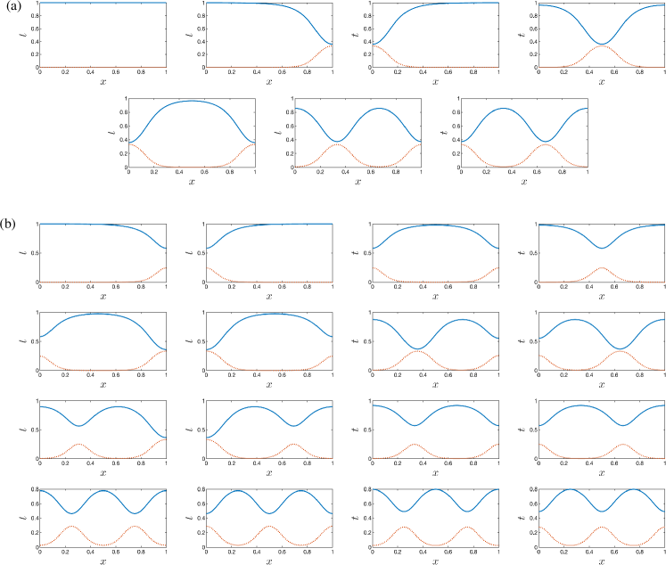
Figure 1: Steady states of the classical Gray-Scott model in the domain $\Omega=(0,1)$, subject to the Neumann boundary condition, with parameter values $D_{u}=5\times 10^{-4}$ and $D_{v}=2.5\times 10^{-4}$, $f=y_{0}=0.04$, and $k=0.065$, computed in [15]: (a) Linearly stable steady states ($u$ : solid line, $v$: dashed line). (b) Linearly unstable steady states ($u$ : solid line, $v$: dashed line).

For the classical Gray-Scott model (where $\epsilon=0$), stationary spatial patterns correspond to non-uniform steady states of the system [15]. Additionally, traveling patterns exist, which correspond to traveling wave solutions [29]. In [15], the authors compute steady states of the classical Gray-Scott model in the domain $\Omega=(0,1)$ subject to the Neumann boundary condition. The parameter values used are $D_{u}=5\times 10^{-4}$ and $D_{v}=2.5\times 10^{-4}$, $f=y_{0}=0.04$, and $k=0.065$. It shows that, under these parameter values, in addition to the trivial uniform steady state $(u,v)=(0,1)$, the classical Gray-Scott model has $6$ non-uniform linearly stable steady-state and $16$ linearly unstable nonuniform steady-state, shown in Fig. 1.

To explore pattern formation in the variational Gray-Scott model for different $\epsilon$, we use these 23 steady states of the classical Gray-Scott model as the initial conditions for $(u,v)$ [15]. The initial conditions of $p$ and $y$ are taken as

$$p_{0}(x)=1,\quad y_{0}(x)=f.$$ (27)

We’ll investigate the evolution of solution with different $\epsilon$. Since the initial concentration of species $X$ is $y_{0}/\epsilon$, for smaller $\epsilon$, more $X$ exist and the total mass $C$, defined in (21), is also larger. We consider $\epsilon=10^{-2}$, $10^{-4}$, and $10^{-6}$, corresponding to a relatively large $\epsilon$, an intermediate-sized $\epsilon$,and a significantly small $\epsilon$, respectively.

3.1 $\epsilon=10^{-2}$: relatively large $\epsilon$

We first consider a relatively large $\epsilon$ by taking $\epsilon=10^{-2}$. Fig. 2(a) - (b) shows the time evolution of different initial conditions for $\epsilon=10^{-2}$, visualized by $u(x,t)$. The initial conditions in Fig. 2(a) correspond to linearly stable steady states of the classical Gray-Scott model, while those in Fig. 2(b) correspond to linearly unstable steady states.

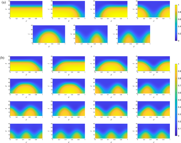
Figure 2: (a) Numerical results for the variational Gray-Scott model with $\epsilon=10^{-2}$ using linearly stable steady states of the classical Gray-Scott model as initial conditions. (b) Numerical results for the variational Gray-Scott model with $\epsilon=10^{-2}$ using linearly unstable steady states of the classical Gray-Scott model as initial conditions

The simulation result shows that, for relatively large $\epsilon$, all initial conditions, including the one with $(u,v)=(1,0)$, converge to the uniform interior steady state ${\bm{u}}_{2}$, as the concentration of $U$ will decrease around $0$. As a result, any non-uniform patterns in the limiting system are destroyed in a relatively short time for a relatively large $\epsilon$.

3.2 $\epsilon=10^{-4}$: Intermediate-sized $\epsilon$

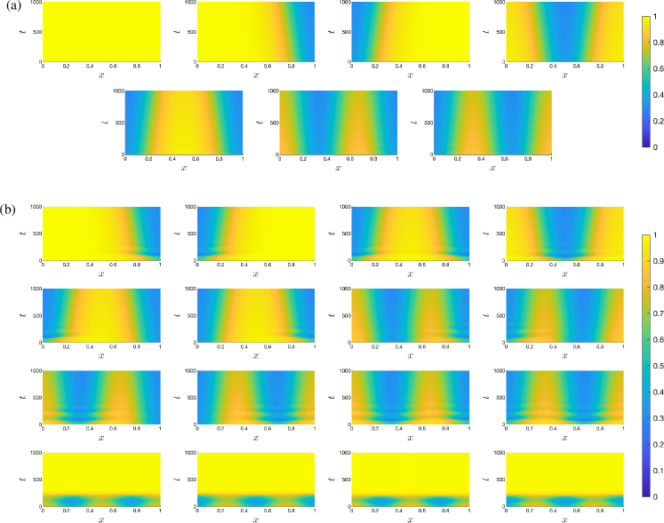
Figure 3: (a) Numerical results for the variational Gray-Scott model with $\epsilon=10^{-4}$ using linearly stable steady states of the classical Gray-Scott model as initial conditions. (b) Numerical results for the variational Gray-Scott model with $\epsilon=10^{-4}$ using linearly unstable steady states of the classical Gray-Scott model as initial conditions.

Next, we consider a intermediate-sized $\epsilon$, $\epsilon=10^{-4}$. The time evolution of different initial conditions for $\epsilon=10^{-4}$, visualized by $u(x,t)$, are shown in Fig.3(a) - (b). The initial conditions in Fig. 3(a) correspond to linearly stable steady states of the classical Gray-Scott model, while those in Fig. 3(b) correspond to linearly unstable steady states. Unlike the case of $\epsilon=10^{-2}$, the initial condition with $(u,v)=(1,0)$ can converge to the boundary steady state, which indicates the stability of the boundary steady state for small $\epsilon$. There are four initial conditions converge to the boundary steady state ${\bm{u}}_{1}$ quickly. Other initial conditions tend to converge to the interior steady state ${\bm{u}}_{2}$ as the concentration of $U$ decreases. However, the convergence is very slow, and non-uniform patterns can persist for a long time. Non-stationary patterns are still observable at $t=1000$.

\begin{overpic}[width=173.44534pt]{vu_os_1e-4_central.eps} \put(-8.0,75.0){(a)} \end{overpic}

\begin{overpic}[width=173.44534pt]{vu_os_1e-4_total_mass.eps} \put(-8.0,75.0){(b)} \end{overpic}

Figure 4: Oscillation behavior for the solution with initial condition corresponding to the unstable solution 4. (a) Evolution of $u(0.5,t)$ and $v(0.5,t)$ with respect to time. (b) Evolution of total mass of $u$ and $v$ with respect to time.

More interestingly, for $\epsilon=10^{-4}$, we observe oscillated solutions during the time evolution. In the original paper on the Gray-Scott model [26], Gray and Scott demonstrate that the system exhibits chemical oscillations even without diffusion. To illustrate the oscillation in the variational Gray-Scott model, we examine the solution with the initial condition corresponding to the linearly unstable solution 4 ((fourth image in Fig. 3(b))) in detail. Fig. 4(a)-(b) show the evolution of $u(0.5,t)$ and $v(0.5,t)$, as well as the total mass of $u$ and $v$, respectively. The plots show the damped oscillations in the concentration of $u$ and $v$, which is similar to the phenomenon reported in Fig. 4 in [26] for the irreversible Gray-Scott model without diffusion. After the oscillation, the solution behavior is similar to the solution with the initial condition corresponding to the stable solution 3 (fourth image in Fig. 3(a)).

3.3 $\epsilon=10^{-6}$: significantly small $\epsilon$

Next, we consider $\epsilon=10^{-6}$, a significantly small $\epsilon$. Fig. 5 shows the simulation results for $\epsilon=10^{-6}$, visualized by $u(x,t)$. Again, the initial conditions in Fig. 5 (a) correspond to linearly stable steady states of the classical Gray-Scott model, while those in Fig. 5 (b) correspond to linearly unstable steady states.

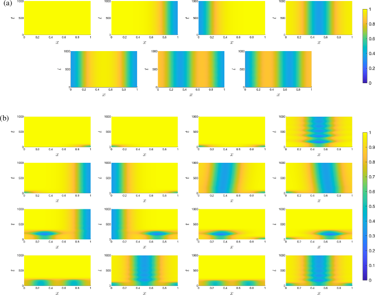
Figure 5: (a) Numerical results for the variational Gray-Scott model with $\epsilon=10^{-6}$ using linearly stable steady states of the classical Gray-Scott model as initial conditions. (b) Numerical results for the variational Gray-Scott model with $\epsilon=10^{-6}$ using linearly unstable steady states of the classical Gray-Scott model as initial conditions.

Like the case with $\epsilon=10^{-4}$, the initial condition with $(u,v)=(1,0)$ converges to the boundary steady state quickly. Additionally, more initial conditions will converge to boundary steady state quickly, compared with the case of $\epsilon=10^{-4}$.

For the initial conditions corresponding to 6 non-uniform linearly stable steady states in the classical Gray-Scott model, the profile of $u$ and $v$ are almost unchanged. In other words, these linearly stable stationary patterns in the classical Gray-Scott model can be stabilized as transient states in the variational model for a very long time when $\epsilon$ is significantly small. We can view these solutions as quasi-steady states or quasi-stable patterns as the $(u,v)$-components of the solution is unchanged. Fig. 6 shows the concentrations of $U$, $V$, $P$, and $X$ at $t=0$ and $t=1000$ for the initial condition associated with the non-uniform linearly stable solution 5. It can be observed that although the concentrations of $U$ and $V$ remain unchanged, the concentration of $P$ decreases while $X$ increases by the same amount. The effective dynamics of the whole system is to transform $X$ to $P$. From the numerical experiments, one can expect the system will reach the interior steady $u_{2}$ at the end as the concentration of $P$ increases and $X$ decreases. However, since the initial concentration of $X$ is much larger than that of $P$, a significant time is needed to reach the steady state. Consequently, the spatial pattern can be stabilized for a long time if the concentration of $X$ is large, i.e., $y(x)\approx f$. Additionally, there are four initial conditions, corresponding to linearly unstable steady-state 5, 6, 9, and 10, which will initially evolve towards a quasi-steady state and will remain unchanged in the $(u,v)-$components for a long time. The simulation results indicate that the variational Gray-Scott model can capture the formation of stationary pattern in the irreversible Gray-Scott model.

\begin{overpic}[width=212.47617pt]{Sol2_1e-6_t_0.png} \put(0.0,65.0){(a)} \end{overpic}

\begin{overpic}[width=212.47617pt]{Sol2_1e-6_t_1000.png} \put(0.0,65.0){(b)} \end{overpic}

Figure 6: Concentration of each species at $t=0$ and $t=1000$. Clearly, the profile of $u$ and $v$ is almost unchanged. But the concentration of $P$ increases significantly and $X$ decreases.

\begin{overpic}[width=173.44534pt]{UV_central_unstable_4.eps} \put(-8.0,75.0){(a)} \end{overpic}

\begin{overpic}[width=173.44534pt]{UV_total_mass_unstable_4.eps} \put(-8.0,75.0){(b)} \end{overpic}

Figure 7: Oscillation behavior for the solution with initial condition corresponding to the unstable solution 4. (a) Evolution of $u(0.5,t)$ and $v(0.5,t)$ with respect to time. (b) Evolution of total mass of $u$ and $v$ with respect to time.

Similar to the case with $\epsilon=10^{-4}$, we observe damped oscillation in the concentrations of $u$ and $v$ when the initial condition corresponds to unstable steady-state 4, 14, 16. Fig. 4(a)-(b) show the evolution of $u(0.5,t)$ and $v(0.5,t)$, as well as the total mass of $u$ and $v$, respectively, for the solution with the initial condition corresponding to the unstable solution 4. Compared with $\epsilon=1e-4$, the damping effect is smaller and more oscillations can be observed. All oscillated solutions will reach stable solution 3 after a long time.

Moreover, we observed two traveling-wave-like solutions when the initial condition corresponds to unstable solutions 7 and 8. The existence of traveling wave solution is one of the most interesting phenomena in the classical Gray-Scott model [39, 25, 40, 29]. These are solutions with the form $u(x,t)=U(z),v(x,t)=V(z)$ with $z=x-ct$ for some constant $c$. As shown in Fig. 5, after some initial evolution, two solutions exhibit a traveling-wave-like behavior. Fig. 8 shows the profile of $u$ in one of the traveling wave-like solutions at $t=200.400,600,800$ and $1000$. Strictly speaking, it is not a traveling wave, as the profile of $u$ is also changed slightly. This might be due to the boundary effect. Fig. 8(b) shows the location of $\min(u)$, which shows a travelling-wave-like behavior. It remains an open question whether real traveling wave solutions exist in the variational Gray-Scott model, which will be investigated in future work.

\begin{overpic}[width=195.12767pt]{travel_wave_u_sol_1.eps} \put(-2.0,75.0){(a)} \end{overpic}

\begin{overpic}[width=186.45341pt]{Loc_min_u_1e-6_travel_wave.eps} \put(-8.0,76.0){(b)} \end{overpic}

Figure 8: (a). A traveling-wave-like solution for $\epsilon=10^{-6}$, shown by profile of $u$ at $t=200.400,600,800$ and $1000$. (b)Location of $\min(u)$ in two traveling-wave-like solutions.

The simulation result suggested that the variational Gray-Scott model can capture various pattern formation phenomena in classical Gray-Scott model, including steady patterns, oscillated patterns, and traveling-wave-like patterns when $\epsilon$ is significantly small. These patterns appear in the variational model as transient states before the system reach to the uniform steady state. It worth mentioning that the classical two-species Gray-Scott model is a subsystem of the four-species variational Gray-Scott model. In this variational model, the concentration of species $X$ is significantly larger than that of the other species, so the dynamics of the system are predominantly governed by the effective reaction $X\ce{<=>}P$. The initial condition of $U$ and $V$ will determine the dynamics either transform $X$ to $P$ or $P$ to $X$. In the current study, since the concentration of $P$ is taken as $1$, which is much smaller than that of $X$, the system will converge to the boundary steady state quickly if essential dynamics is $P$ to $X$. We can observe the pattern formation for a significant long time if the essential dynamics is $X$ to $P$. We’ll investigate the effects of the initial concentration of $P$ in future work.

4 Stability of Trivial steady-states in variational Gray-Scott model

In this section, we provide some theoretical analysis of the numerical results in the previous section by analyzing the stability of two uniform steady states of the variational Gray-Scott model (17) for fixed $\epsilon$.

Although the variational Gray-Scott model comprises four terms - U, V, P, and X, due to the conservation law, the degrees of freedom in the system are constrained to three, corresponding to three reaction trajectories $R_{i}$. Specifically, based on Eqs. (5), the perturbation in the stability analysis satisfies

$$\bm{s}=(-s_{1}-s_{3},s_{1}-s_{2},s_{2},\epsilon s_{3})$$

where $s_{i}\in\mathbb{R}$ for $i=1,2,3$. Thus we define the perturbation manifold as follows:

$$\mathcal{S}_{1}:=\operatorname{span}\{\bm{s}_{1},\bm{s}_{2},\bm{s}_{3}\},~{}\bm{s}_{1}:=(0,-1,1,0),\bm{s}_{2}:=(-1,0,0,\epsilon),\bm{s}_{3}:=(-1,1,0,0).$$ (28)

4.1 Stability of the interior steady-state

For the interior steady state, we ascertain that it is a local minimum of the system based on the following proposition:

Proposition 4.1.

For any $\epsilon>0$, the interior steady state

$$\bm{u}_{2}=(u^{s}_{2},v^{s}_{2},p^{s}_{2},y^{s}_{2})=\left(\frac{\epsilon}{\lambda}C,~{}\frac{1}{\lambda}C,~{}\frac{k+f}{\epsilon\lambda}C,~{}\frac{f\epsilon}{\lambda}C\right)$$ (29)

is a local minimum point of the free energy $\mathcal{F}$ on the manifold ${\bm{u}}_{0}+\mathcal{S}_{1}$, where ${\bm{u}}_{0}=(u_{0},v_{0},p_{0},y_{0}/\epsilon)$ is the initial condition.

Proof.

Without loss of generality, we perturb $\bm{u}_{2}$ along the direction of $\bm{s}_{1}$ of the three-dimensional manifold $\mathcal{S}_{1}$ (a similar analysis applies to other directions) and obtain:

$$\frac{\mathrm{d}E[\bm{u}_{2}+\delta\bm{s}_{1}]}{\mathrm{d}\delta}=\ln(p^{s}_{2}+\delta)+\sigma_{p}-\ln(v^{s}_{2}-\delta)-\sigma_{v}.$$ (30)

By the definition of $\sigma_{p}$ and $\sigma_{v}$, we conclude that $\delta=0$ is the unique solution of $\frac{\mathrm{d}E[\bm{u}_{2}+\delta\bm{s}_{1}]}{\mathrm{d}\delta}=0$, indicating the critical point. Furthermore, by computing the second variation, we have:

$$\frac{\mathrm{d}^{2}E[\bm{u}_{2}+\delta\bm{s}_{1}]}{\mathrm{d}\delta^{2}}=\frac{1}{p^{s}_{2}+\delta}+\frac{1}{v^{s}_{2}-\delta}.$$ (31)

Since $v^{s}_{2},p^{s}_{2}>0$ for any $\epsilon>0$, $\frac{\mathrm{d}^{2}E[\bm{u}_{2}+\delta\bm{s}_{1}]}{\mathrm{d}\delta^{2}}\big{|}_{\delta=0}>0$, indicating that this steady state is a local minimum in the $\bm{s}_{1}$ direction, similarly for other directions. ∎

Next, we examine the interior steady state and its behavior as $\epsilon$ approaches zero. To visualize this, we plot the energy landscape around this steady state in three directions on $\mathcal{S}_{1}$ shown in Fig. 1. While the behavior of $\bm{s}_{1}$ remains stable, for $\bm{s}_{2}$ and $\bm{s}_{3}$, we observe a notable change as $\epsilon$ diminishes: the stable region contracts significantly. Essentially, the inflection point approaches the steady state in this direction.

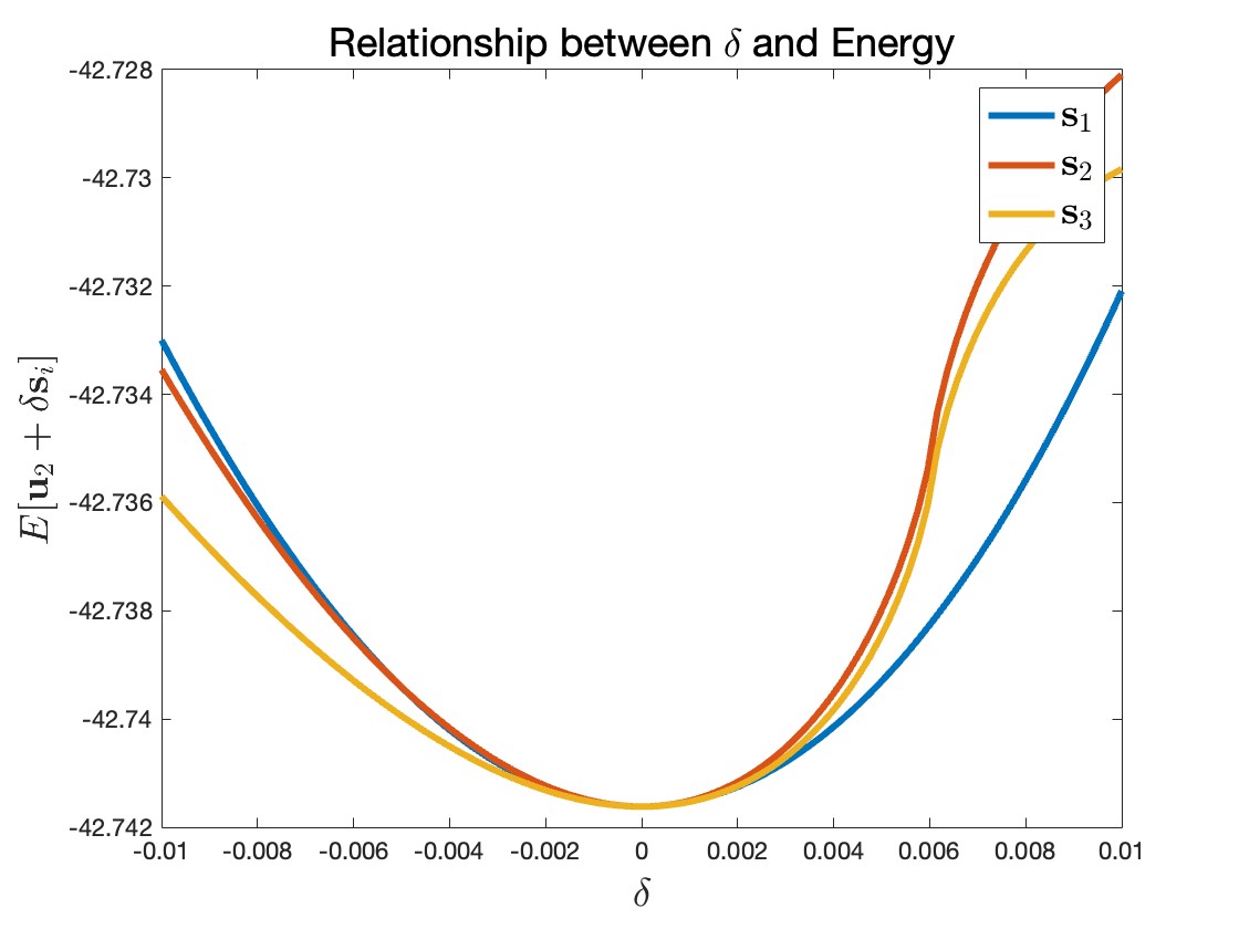
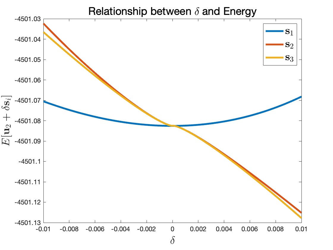
Figure 9: Energy Landscape for $\epsilon=0.01$ and $\epsilon_{3}=0.0001$ along the $\bm{s}_{i}$ directions relative to the interior steady state.

The reason for this phenomenon is the proximity of $u_{2}^{s}$ to zero when $\epsilon$ is small. As previously mentioned, this term is of $\mathcal{O}(\epsilon)$. Examining the second variation in the $\bm{s}_{3}$ direction reveals:

$$\frac{\mathrm{d}^{2}E[\bm{u}_{2}+\delta\bm{s}_{3}]}{\mathrm{d}\delta^{2}}=\frac{1}{v^{s}_{2}+\delta}+\frac{1}{u^{s}_{2}-\delta}.$$ (32)

In the $\bm{s}_{3}$ direction, there are four inflection points, one of which occurs at

$$\delta={u^{s}_{2}}=\mathcal{O}(\epsilon)$$

very close to zero when $\epsilon$ is small.

In summary, we have established that the interior steady state remains stable for all $\epsilon>0$. However, as $\epsilon$ decreases, the stable region also becomes smaller. Nonetheless, it is still challenging for the system to escape from the steady state, as it would require $\delta>u^{s}_{2}$, which would result in $u<0$, an impossible scenario. Therefore, even for very small $\epsilon$, if the initial data is not far away from the steady state, the system will still converge to this interior steady state. When $\epsilon$ is small, ensuring that the initial conditions are not too far from the steady state requires $p$ to be of order $\epsilon^{-1}$, meaning $p$, a real term in the system, must have a significant presence.

4.2 Stability of the boundary steady-state

For the boundary steady state, the stability analysis diverges from that of the interior steady state. Employing the same analysis method, we observe that this is not even a critical point. Recall $\bm{s}_{1}=(-1,1,0,0)\in\mathcal{S}_{1}$, then:

$$\frac{\mathrm{d}E[\bm{u}_{1}+\delta\bm{s}_{1}]}{\mathrm{d}\delta}=\ln(v^{s}_{2}+\delta)+\sigma_{v}-\ln(u^{s}_{2}-\delta)-\sigma_{u}=\ln\delta+\sigma_{v}-\ln(u^{s}_{2}-\delta)-\sigma_{u}.$$ (33)

This expression tends to infinity as $\delta\to 0^{+}$, indicating it is not a critical point.

The reason for employing a different stability analysis lies in the disappearance of $V$ and $P$ at this steady state. Consequently, the first and second reactions cease to exist:

$$\ce{U+2V<=>[1][\epsilon]3V},\quad\ce{V<=>[k+f][\epsilon]P}.$$ (34)

In other words, perturbations in the first and second reactions are no longer feasible, leaving perturbations only viable for the third reaction. This restriction results in a one-dimensional perturbation space:

$$\mathcal{S}_{2}:=\operatorname{span}\{(-1,0,0,\epsilon)\}.$$

Proposition 4.2.

For any $\epsilon>0$, the boundary steady state

$$\bm{u}_{1}=(u^{s}_{1},v^{s}_{1},p^{s}_{1},y^{s}_{1}):=\left(\frac{\epsilon}{\epsilon+f}C,~{}0,~{}0,~{}\frac{f\epsilon}{(\epsilon+f)}C\right),$$ (35)

is a local minimum point of the free energy $\mathcal{F}$ on the manifold ${\bm{u}}_{0}+\mathcal{S}_{2}$, where ${\bf u}_{0}=(u_{0},v_{0},p_{0},y_{0}/\epsilon)$ is the initial condition.

Proof.

The proof follows a similar structure to that of Proposition 4.1. ∎

Therefore, the stability of the boundary steady state only pertains to the third reaction. It exhibits what we term as virtual stability, meaning the steady state is stable for the last reaction but not for the first two. However, since the first and second reactions do not exist in the entire system, the system is considered stable overall. The reason for labeling this as ‘virtual’ is that the third reaction is artificial and virtual, as it does not exist in the classical Gray-Scott models defined by Eq. (2).

Overall, we observe that the interior steady state is stable, while the boundary steady state is considered virtually stable. This virtual stability arises when V and X are scarce or nonexistent, which occurs when $\epsilon$ is small, as demonstrated in Section 3. In such cases, the initial terms of P and V occupy only a fraction of $\epsilon$ in the entire system, while the term X dominates almost entirely. This scenario satisfies the conditions for virtual stability, leading the system to converge to the boundary steady state.

Furthermore, we aim to elucidate that even though the boundary steady state is only a local minimum for the third reaction (i.e., $(-1,0,0,\epsilon)$ is not stable in the $(-1,1,0,0)$ and $(0,1,-1,0)$ directions), it still behaves as a nearly local minimum when $\epsilon$ is small and X dominates the system. In such cases, when the system comprises $\mathcal{O}(1)$ amounts of U, V, and P, and $\mathcal{O}(\epsilon^{-1})$ of X, the third reaction occupies almost the entire system. Additionally, the first and second reactions account for only a fraction of $\epsilon$ in the system. When considering perturbations in this context, denoting the direction as

$$\bm{s}=(-1,0,0,\epsilon)+(-\epsilon,0,\epsilon,0),$$

direct calculation reveals that:

$$\lim_{\epsilon\to 0}\frac{\mathrm{d}E[\bm{u}_{1}+\delta\bm{s}]}{\mathrm{d}\delta}=\lim_{\epsilon\to 0}\frac{\mathrm{d}E[\bm{u}_{1}+\delta{(-1,0,0,\epsilon)}]}{\mathrm{d}\delta}=0.$$ (36)

Additionally, numerical results further support this assertion, as shown in Figure 10. The boundary steady state exhibits near-stability when X dominates almost the entire system. This is primarily because most reactions in this scenario are governed by the third reaction, which is stable for the boundary steady state. Consequently, the entire system behaves as if approaching a local minimum.

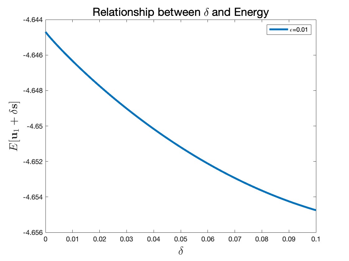
Figure 10: Numerical results demonstrating near-stability when X dominates almost the entire system.

In summary, when $\epsilon$ is not very small, it does not satisfy the stable condition for virtual stability, leading to convergence to the interior steady state. Additionally, it is straightforward to verify that the set $\mathbf{\delta}=(\delta_{1},\delta_{2},\delta_{3})$ satisfies:

$$\frac{\mathrm{d}E[\bm{u}_{1}+\delta_{1}(-1,1,0,0)+\delta_{2}(0,-1,1,0)+\delta_{3}(-1,0,0,\epsilon)]}{\mathrm{d}\mathbf{\delta}}=0.$$ (37)

This equation can be rewritten as:

$$\begin{cases}\frac{u_{1}^{s}-\delta_{1}-\delta_{3}}{\delta_{1}-\delta_{2}}=\epsilon\\ \frac{\delta_{1}-\delta_{2}}{\delta_{2}}=\frac{\epsilon}{f+k}\\ \frac{\epsilon(u_{1}^{s}-\delta_{1}-\delta_{3})}{y_{1}^{s}+\epsilon\delta_{3}}=\frac{\epsilon}{f}.\end{cases}$$ (38)

This system has a unique nonzero solution, denoted as:

$$\bm{u}_{1}+\delta_{1}(-1,1,0,0)+\delta_{2}(0,-1,1,0)+\delta_{3}(-1,0,0,\epsilon)=\bm{u}_{2}.$$

The theoretical analysis is consistent with the numerical results. When $\epsilon$ is large, all initial conditions converge to ${\bm{u}}_{2}$ as it is stable. However, for a significantly small $\epsilon$, the gradient flow dynamics select the boundary steady state ${\bm{u}}_{1}$ for some unstable steady states due to the virtual stability of the boundary steady state in this case. In other words, both trivial steady states become ”stable.” For some unstable steady states, the system will choose the boundary steady state. Furthermore, since the initial condition is close to the boundary steady state but far from the interior steady state due to the large value of $X$, the system will quickly converge to the boundary steady state. However, it will take a long time to converge to the interior steady state, which cause the persistence of the non-uniform patterns.

5 Pattern persistence time v.s. $\epsilon$

Simulation results in section 3 show that for relatively large $\epsilon$, all initial conditions associated with the steady states of the classical Gray-Scott model will converge to the uniform interior steady state in the variational Gray-Scott model. However, for smaller $\epsilon$, some of these initial conditions will converge to the boundary steady state quickly, and some will converge to the interior steady state slowly. The persistence of non-uniform patterns can be observed for a very long time in the latter case. In this section, we study the pattern persistence time in the variational Gray-Scott model with respect to $\epsilon$.

We consider two initial conditions, which correspond to the non-uniform linearly stable solution 6 (the last solution in Fig. 1(a)) and the linearly unstable solution 3 (the third solution in Fig. 1(b)). The first one will always converge to the interior steady state, at least when $\epsilon$ is not too small. The second one will converge to the interior steady state for large $\epsilon$, but converge to the boundary steady state for small $\epsilon$. We define the pattern time as

$$T=\inf\{t~{}|~{}\max\{\max u(t)-\min u(t),~{}\max v(t)-\min v(t)\}\leq a\}$$

with $a$ being significantly small since the vanishing of the pattern indicates that both $u$ and $v$ are close to constant functions. We pick $a=0.05$ throughout this section. Fig. 11 shows the relationship between the pattern persistence time and $\epsilon$ for these two initial conditions.

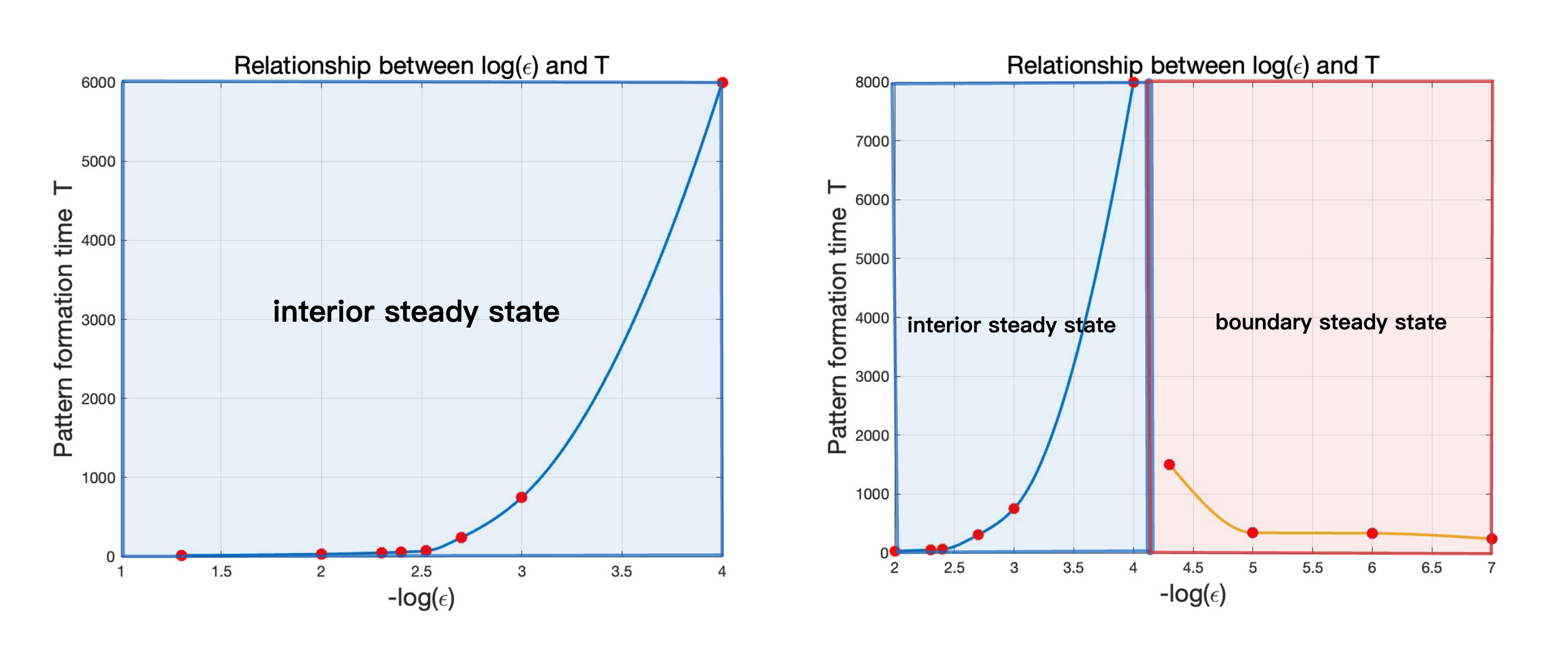
Figure 11: The Pattern persistence time and $\epsilon$ for a stable and an unstable initial condition, where pattern formation time is the first time when $\max\{\max u(t)-\min u(t),\max v(t)-\min v(t)\}\leq 0.05$.

For the linearly stable solution 6, the pattern persistence time increases as $\epsilon$ decreases, and is of the order $\mathcal{O}(\epsilon^{-1})$. For the linearly unstable solution 3, it converges to the interior state for relatively large $\epsilon$, and the pattern persistence time also increases with decreasing $\epsilon$, following the order $\mathcal{O}(\epsilon^{-1})$. However, the initial condition converges to the boundary steady state for large $\epsilon$, and the initial pattern will be destroyed faster for smaller $\epsilon$. The result is consistent with the previous simulation and analysis.

To have pattern formation in the variational Gray-Scott model, one need to have some particular initial condition such that the variational model converges to the interior steady state, in which all $X$ will convert to $P$. The pattern is maintained if the concentration of $X$ stays large, analogous to the continuous feed of $U$ in the classical Gray-Scott model. The conclusion is similar to that in a recent paper [41] on a slightly different thermodynamically consistent three-species reaction-diffusion model, in which the authors show that for a finite system, a specific Turing pattern exists only within a finite range of total molecule number, and the presence of third species stabilize the Turing pattern of the two species.

6 Conclusions

In this paper, we study the pattern formation of a thermodynamically consistent variational Gray-Scott model, derived by an energetic variational approach, in one dimension. The variational Gray-Scott model includes a virtual term $X$ and reversible reactions to the classical Gray-Scott model, transforming the system into a thermodynamically consistent closed system. The classical Gray-Scott model can be viewed as a subsystem of the variational Gray-Scott model when the reverse reaction rate $\epsilon$ tends to zero. By decreasing $\epsilon$, we observed that the stationary pattern in the classical Gray-Scott model can appear as the transient state in the variational model when $\epsilon$ is significantly small. Additionally, the variational model admits oscillated and traveling-wave-like solutions for small $\epsilon$. The results show the capability of variational model in capturing pattern formation.

We also analyze the stability of two uniform steady states, an interior steady state and a boundary steady state, in the variational Gray-Scott model. Although the interior steady state is always stable, the stability region becomes significantly smaller as $\epsilon$ decreases. In the meantime, the boundary steady state is virtually stable, i.e., is stable with respect to the third reaction $U\ce{<=>}X$. For certain initial conditions, since the concentration of $X$ (at order $\mathcal{O}(\epsilon^{-1})$) is much larger than other species (at the order of $\mathcal{O}(1)$) for small $\epsilon$, the gradient flow dynamics will drive the system to the boundary steady state. In order to observe pattern formation, one needs a special initial condition such that the dynamics will not converge to the boundary steady state.

The variational Gray-Scott model offers a new mathematical framework for understanding pattern formation from a thermodynamic perspective. The numerical simulation and theoretical analysis suggest that pattern formation is maintained by the presence of species $X$, i.e., the continuous input of $U$ in the classical Gray-Scott model. The initial condition determines the effective direction of the reaction network, and the pattern formation can only occur if the network continuously generates the inert product $P$. However, several open questions remain that are worth exploring, including: 1) Investigating the effect of varying the scale of small parameter $\epsilon_{i}$ in the reaction network (4); 2) Analyzing the role of $P$ in pattern formation; 3). Examining more general initial conditions, beyond the steady states typically used in Gray-Scott models. We’ll study these open questions in future work.

References

- [1] J. D. Murray, Spatial models and biomedical applications, Mathematical Biology.
- [2] P. Maini, H. Othmer, Mathematical models for biological pattern formation, in: Mathematics Inspired by Biology, Springer, 2001, pp. 153–176.
- [3] A. Turing, The chemical basis of morphogenesis: Philosophical transactions of the roy al society of london. ser. b, in: Biol. Sci, Vol. 237, 1952.
- [4] D. M. Umulis, H. G. Othmer, The role of mathematical models in understanding pattern formation in developmental biology, Bulletin of mathematical biology 77 (5) (2015) 817–845.
- [5] P. Maini, R. Baker, C. Chuong, The turing model comes of molecular age, Science’s STKE 2006 (335) (2006) pe30.
- [6] H. Othmer, S. Dunbar, W. Alt, Models of dispersal in biological systems, Journal of Mathematical Biology 26 (3) (1988) 263–298.
- [7] H. Othmer, L. Scriven, Instability and dynamic pattern in cellular networks, Journal of Theoretical Biology 32 (3) (1971) 507–537.
- [8] H. Othmer, K. Painter, P. Maini, Multiscale models of developmental systems, Current Opinion in Genetics & Development 16 (4) (2006) 391–399.
- [9] S. Kondo, T. Miura, Reaction-diffusion pattern formation in development, Dynamics of patterning (2010) 103–126.
- [10] H. Meinhardt, A. Gierer, Pattern formation by local self-activation and lateral inhibition, Bioessays 22 (8) (2000) 753–760.
- [11] G. F. Oster, J. D. Murray, A. Harris, Mechanical aspects of mesenchymal morphogenesis, Development 78 (1) (1983) 83–125.
- [12] R. J. Field, R. M. Noyes, Oscillations in chemical systems. iv. limit cycle behavior in a model of a real chemical reaction, The Journal of Chemical Physics 60 (5) (1974) 1877–1884.
- [13] I. R. Epstein, J. A. Pojman, An introduction to nonlinear chemical dynamics: oscillations, waves, patterns, and chaos, Oxford university press, 1998.
- [14] J. Langer, Models of pattern formation in first-order phase transitions, in: Directions in condensed matter physics: Memorial volume in honor of shang-keng ma, World Scientific, 1986, pp. 165–186.
- [15] W. Hao, C. Xue, Spatial pattern formation in reaction–diffusion models: a computational approach, Journal of mathematical biology 80 (2020) 521–543.
- [16] S. Wu, B. Yu, Y. Tu, L. Zhang, Solution landscape of reaction-diffusion systems reveals a nonlinear mechanism and spatial robustness of pattern formation, arXiv preprint arXiv:2408.10095.
- [17] W. Hao, S. Lee, Y. J. Lee, Companion-based multi-level finite element method for computing multiple solutions of nonlinear differential equations, Computers & Mathematics with Applications 168 (2024) 162–173.
- [18] H. Zheng, Y. Huang, Z. Huang, W. Hao, G. Lin, Hompinns: Homotopy physics-informed neural networks for solving the inverse problems of nonlinear differential equations with multiple solutions, Journal of Computational Physics 500 (2024) 112751.
- [19] W. Hao, J. Hesthaven, G. Lin, B. Zheng, A homotopy method with adaptive basis selection for computing multiple solutions of differential equations, Journal of Scientific Computing 82 (1) (2020) 19.
- [20] Y. Wang, W. Hao, G. Lin, Two-level spectral methods for nonlinear elliptic equations with multiple solutions, SIAM Journal on Scientific Computing 40 (4) (2018) B1180–B1205.
- [21] Y. Huang, W. Hao, G. Lin, Hompinns: Homotopy physics-informed neural networks for learning multiple solutions of nonlinear elliptic differential equations, Computers & Mathematics with Applications 121 (2022) 62–73.
- [22] J. E. Pearson, Complex patterns in a simple system, Science 261 (5118) (1993) 189–192.
- [23] X. Wang, J. Shi, G. Zhang, Bifurcation and pattern formation in diffusive klausmeier-gray-scott model of water-plant interaction, Journal of Mathematical Analysis and Applications 497 (1) (2021) 124860.
- [24] X. Chen, X. Lai, C. Qin, Y. Qi, Y. Zhang, Multiple-peak traveling waves of the gray-scott model, Mathematics in Applied Sciences and Engineering 4 (3) (2023) 154–171.
- [25] A. Doelman, T. Kaper, P. Zegeling, Pattern formation in the one-dimensional gray-scott model, Nonlinearity 10 (2) (1997) 523.
- [26] P. Gray, S. K. Scott, Autocatalytic reactions in the isothermal, continuous stirred tank reactor: Oscillations and instabilities in the system a+ 2b→ 3b; b→ c, Chemical Engineering Science 39 (6) (1984) 1087–1097.
- [27] P. Gray, S. K. Scott, Chemical oscillations and waves, Chaos: An Interdisciplinary Journal of Nonlinear Science 23 (2) (1984) 025112.
- [28] G. Hu, Z. Qiao, T. Tang, Moving finite element simulations for reaction-diffusion systems, Advances in Applied Mathematics and Mechanics 4 (3) (2012) 365–381.
- [29] Y. Qi, Y. Zhu, The travelling wave of gray-scott systems–existence, multiplicity and stability, Journal of Biological Dynamics 11 (sup2) (2017) 379–399.
- [30] H. Nakao, Collective dynamics in non-linear systems of coupled oscillators, Nonlinearity 23 (1) (2010) R1.
- [31] W. Li, H. Zhang, X. Zhang, J. Guo, Turing patterns in multiplex networks, Physica A: Statistical Mechanics and its Applications 470 (2017) 285–292.
- [32] J. Liang, N. Jiang, C. Liu, Y. Wang, T. Zhang, On a reversible gray-scott type system from energetic variational approach and its irreversible limit, Journal of Differential Equations 309 (2022) 427–454.
- [33] M. Giga, A. Kirshtein, C. Liu, Variational modeling and complex fluids, Handbook of mathematical analysis in mechanics of viscous fluids (2017) 1–41.
- [34] Y. Wang, C. Liu, Some recent advances in energetic variational approaches, Entropy 24 (5) (2022) 721.
- [35] H. Ge, H. Qian, Dissipation, generalized free energy, and a self-consistent nonequilibrium thermodynamics of chemically driven open subsystems, Physical Review E—Statistical, Nonlinear, and Soft Matter Physics 87 (6) (2013) 062125.
- [36] G. Falasco, R. Rao, M. Esposito, Information thermodynamics of turing patterns, Physical review letters 121 (10) (2018) 108301.
- [37] Y. Wang, C. Liu, P. Liu, B. Eisenberg, Field theory of reaction-diffusion: Law of mass action with an energetic variational approach, Physical Review E 102 (6) (2020) 062147.
- [38] D. Kondepudi, I. Prigogine, Modern thermodynamics: from heat engines to dissipative structures, John Wiley & Sons, 2014.
- [39] V. Manukian, On travelling waves of the gray–scott model, Dynamical Systems 30 (3) (2015) 270–296.
- [40] Y. Kyrychko, K. Blyuss, S. Hogan, E. Schöll, Control of spatiotemporal patterns in the gray–scott model, Chaos: An Interdisciplinary Journal of Nonlinear Science 19 (4).
- [41] D. Zhang, C. Zhang, Q. Ouyang, Y. Tu, Free energy dissipation enhances spatial accuracy and robustness of self-positioned turing pattern in small biochemical systems, Journal of the Royal Society Interface 20 (204) (2023) 20230276.