Incorporating external data for analyzing randomized clinical trials: A transfer learning approach
Abstract
Randomized clinical trials are the gold standard for analyzing treatment effects. However, increasing costs and ethical concerns may limit trial recruitment, resulting in insufficient sample sizes and potentially invalid inference. Incorporating external trial data with similar characteristics (treatments, diseases, biomarkers, etc.) into the analysis appears promising for addressing these issues. Transfer learning, which in our context utilizes external trials as the source domain and current trials as the target domain, may offer a viable approach. In this paper, we present a formal framework for applying transfer learning to the analysis of clinical trials, considering three key perspectives: transfer algorithm, theoretical foundation, and inference method. To cover broad types of randomized trials, we study this problem under stratified, or more generally, covariate-adaptive randomization. For the algorithm, we adopt a parameter-based transfer learning approach to enhance the lasso-adjusted stratum-specific estimator developed for estimating the treatment effect. A key component in constructing the transfer learning estimator is deriving the regression coefficient estimation within each stratum, accounting for the bias between source and target data. To provide a theoretical foundation, we derive the convergence rate for the estimated regression coefficients and subsequently establish the asymptotic normality for the transfer learning estimator. Our results show that when external trial data resembles current trial data, the sample size requirements can be reduced compared to using only current trial data. Finally, we propose a consistent nonparametric variance estimator to facilitate inference that is robust to model misspecifications and applicable to various commonly used randomization procedures. Numerical studies demonstrate the effectiveness and robustness of our proposed estimator across various scenarios. Our study highlights the potential of transfer learning in analyzing randomized clinical trials.
Key words: Covariate-adaptive randomization; External trial data; Lasso; Robust inference.
1 Introduction
Randomization is the gold standard in clinical trials and other intervention studies, such as online A/B tests and experiments in development economics. After randomization, a treatment effect estimator that can provide valid inference should be constructed. However, randomized clinical trials may suffer from rising costs, ethical concerns, and recruitment difficulties, especially when the trial involves rare or life-threatening diseases. Consequently, the inference may become invalid due to the lack of sufficient experimental units, i.e., patients enrolled in the trial. To solve this problem, data from external trials are encouraged to assist in analyzing the current trial [FDA, 2022]; for discussions on using external data from observational studies, see related work in Section 1.1. The use of external trial data is most promising when the current trial and the external trial share similar drugs, biomarkers, or treatment procedures. For example, when analyzing the Covidicus trial, researchers leveraged external Recovery trial data to evaluate the efficacy of dexamethasone, a common treatment in both trials, for critically ill COVID-19 patients, although the Bayesian methods used may be sensitive to parametric model settings [Chevret et al., 2022].
The recent development of transfer learning, especially in the field of statistics, offers insights into incorporating external trial data into the analysis of current trial data. Transfer learning [Torrey and Shavlik, 2010] uses information from similar source data to support the analysis of target data. To date, transfer learning has been successfully applied in many fields, such as natural language processing, computer vision, and epidemiology. Due to its empirical success, transfer learning has received considerable attention in statistical disciplines. For example, it has been studied in a variety of problems, such as classification [Cai and Wei, 2021], nonparametric regression [Cai and Pu, 2024], and contextual multi-armed bandits [Cai et al., 2024]. Most relevant to our work, due to the availability of a large number of baseline covariates in modern clinical trials, transfer learning, when applied to high-dimensional problems, has been shown to improve the convergence rate of regression coefficients compared to using only the target data [Li et al., 2022, Tian and Feng, 2023]. Moreover, transfer learning can also improve estimation and inference accuracy in the Gaussian graphical model [Li et al., 2023]. These works inspire us to apply transfer learning to estimating treatment effects in clinical trials, especially in a high-dimensional setting.
While incorporating external trial data through transfer learning is conceptually intuitive, ensuring robust inference is pivotal for its acceptance in clinical trial practice, and this is the mission of our paper. Here, robustness indicates that the inference remains valid even when the working model used to derive the treatment effect estimation is misspecified. Such robustness is desirable when analyzing clinical trial data because the true data generation model is usually unknown. Without using external trial data, the robustness of treatment effect estimators has been extensively studied under various randomization methods. Specifically, under simple randomization, the robustness of different regression estimators has been discussed in several influential papers [Freedman, 2008, Lin, 2013, Yang and Tsiatis, 2001]. In this paper, we focus on covariate-adaptive randomization, which is commonly used in clinical trials to produce a more balanced treatment allocation within strata formed by covariates, such as stratified block randomization [Zelen, 1974]. According to recent surveys, covariate-adaptive randomization is implemented in about 70% of trials [Ciolino et al., 2019]. The inference under covariate-adaptive randomization has been challenging due to the dependence between treatment assignments. Bugni et al. [2018] proposed robust treatment effect estimators based on several regression models adjusting for strata variables. Subsequently, many researchers have adjusted additional baseline covariates in the regression models to further improve efficiency [Ma et al., 2022, Liu et al., 2023, Ye et al., 2023, 2022, Gu et al., 2023]. Notably, under a high-dimensional setting, Liu et al. [2023] applied lasso regression to obtain a lasso-adjusted stratum-specific treatment effect estimator, which is optimal among the class of all regression-adjusted estimators. For more discussion on covariate-adaptive randomization and its inference, please refer to Section 1.1.
To fulfill our mission, challenges from three perspectives need to be tackled: transfer algorithm, theoretical foundation, and inference method. Firstly, a transfer learning approach must be tailored to the context of covariate-adaptive randomization to ensure proper knowledge or feature transfer from the source (external trial) to the target (current trial) data, without compromising the performance on the target task in terms of the robustness of treatment effect estimation. Secondly, providing theoretical guarantees that the treatment effect estimation will benefit from transfer learning is crucial, given that the dependence in treatment assignments across experimental units resulting from covariate-adaptive randomization. Finally, valid inference is critical for accurate treatment effect estimation, which is rarely considered in previous transfer learning research. We expect our transfer learning approach to produce valid inference that is applicable to commonly used randomization methods and robust against model misspecification.
In this paper, we propose a robust treatment effect estimator via transfer learning to address the aforementioned issues. For the first challenge, we apply a parameter-based transfer learning approach [Li et al., 2022] to enhance the lasso-adjusted stratum-specific treatment effect estimator developed for covariate-adaptive randomization. Importantly, this method also strengthens data privacy and security, which is crucial in clinical trials due to the sensitivity of patient information. Specifically, we begin by using lasso regression to obtain regression coefficients from the source data within each stratum. We then correct the bias in these regression coefficients between the source and target data by applying lasso regression to the target data. The target regression coefficient estimator is obtained by adding the bias estimator to the source regression coefficient estimator. Finally, the transfer learning-enhanced treatment effect estimator (referred to hereafter as the transfer learning estimator for simplicity) is constructed by substituting the original regression coefficients in the stratum-specific estimator with these bias-corrected target regression coefficients.
Then, extending the theory for the lasso-adjusted treatment effect estimator in Liu et al. [2023], we establish the norm consistency of the target regression coefficient estimators, which is key to deriving the asymptotic normality for the transfer learning estimator. Under mild conditions, we show that, when the source and target data are similar, the convergence rate of the regression estimators is faster than the convergence rate in Liu et al. [2023]. This result leads to an improvement in inference based on our proposed estimator, which requires fewer units in the target data. Notably, our proposed estimator achieves optimal efficiency for a regression-adjusted estimator under covariate-adaptive randomization with multiple treatments [Gu et al., 2023].
Finally, we facilitate valid inference by developing a consistent nonparametric variance estimator for the transfer learning estimator. In general, inference under transfer learning for high-dimensional data is non-trivial. However, thanks to our framework, we can preserve robust inference for the treatment effect, avoiding negative transfer when incorporating source data. Moreover, the proposed inference procedure is widely applicable to a broad class of covariate-adaptive randomization procedures. Additionally, the robustness of our transfer learning approach can adapt to scenarios where the covariate distributions or functional forms of data generation models may differ between the source and target data.
1.1 Related works
Covariate-adaptive randomization and its inference. Covariate-adaptive randomization aims to provide more balanced treatment allocation with respect to baseline covariates. For example, stratified block randomization [Zelen, 1974] defines sets of strata based on covariates and allocates experimental units in each stratum using block randomization. Minimization methods [Taves, 1974, Pocock and Simon, 1975] have been proposed to balance covariates over their margins. This approach has been generalized to control various types of imbalance measures, including overall and within-stratum imbalance measures [Hu and Hu, 2012, Hu and Zhang, 2020]. Other commonly used covariate-adaptive randomization approaches such as stratified biased coin design [Efron, 1971, Shao et al., 2010] and model-based approaches [Begg and Iglewicz, 1980, Atkinson, 1982]. We refer readers to Rosenberger and Lachin [2015] for a detailed discussion of these methods.
Our theoretical analysis of the inference for the regression-adjusted treatment effect estimators is related to recent studies, which have shown that under covariate-adaptive randomization, regression-adjusted treatment effect estimators are valid for inference. Bugni et al. [2018] proposed robust treatment effect estimators that are resistant to model misspecification with regression adjustment for stratification, which can produce valid inference. With the inclusion of additional baseline covariates, stratum-common and stratum-specific treatment effect estimators have been proposed to improve the efficiency of the estimators [Ye et al., 2023, 2022, Ma et al., 2022]. Gu et al. [2023] showed that the stratum-specific estimator could gain efficiency compared with the stratum-common estimator under multiple treatments, regardless of whether the allocation ratios are the same across strata. In high-dimensional settings, Liu et al. [2023] obtained the regression coefficient estimator by lasso and replaced the original coefficient estimator in stratum-common and stratum-specific estimators to get lasso-adjusted estimators. Under regular conditions on sparsity, they showed that the lasso-adjusted estimators could achieve the same efficiency as the regression-adjusted estimators under two treatments. When the working model is a general function of covariates instead of a linear form, researchers reach a theoretical guarantee for the efficiency gain if the function form is properly estimated [Rafi, 2023, Bannick et al., 2023, Tu et al., 2023].
Transfer learning. Transfer learning is widely applied in many fields, such as computer vision [Wah et al., 2011, Saenko et al., 2010, Donahue et al., 2014], natural language processing [Ruder et al., 2019, Wolf et al., 2020], biomedical analysis [Schweikert et al., 2008, Petegrosso et al., 2017], etc. We refer readers to Pan and Yang [2009], Weiss et al. [2016], Zhuang et al. [2020] for comprehensive surveys on transfer learning. Based on the type of knowledge being transferred, transfer learning problems can be categorized into several subproblems: instance-based, feature-based, parameter-based and relation-based problems [Pan and Yang, 2009]. Our paper focuses on the parameter-based problem as we transfer the regression coefficients from the source data to the target data. Due to its successful empirical performance, transfer learning draws extensive attention in the statistics field. Besides the work we have mentioned, transfer learning has also been applied to statistical problems such as high-dimensional quantile regression [Huang et al., 2022, Jin et al., 2024] and precision medicine [Wu and Yang, 2023].
Bayesian historical borrowing. In many cases, historical trial data with settings similar to the current trial data are available. Including these historical data may improve the precision of estimations in the current trial [Pocock, 1976]. As the treatments usually differ between trials, researchers mainly focused on using historical control data. However, the difference in population distribution may lead to heterogeneity among the historical data and current data. Under the Bayesian framework, researchers proposed several methods to address the issue, such as using power prior [Ibrahim and Chen, 2000, Ibrahim et al., 2015], meta-analytic predictive prior [Schmidli et al., 2014] and hierarchical models [Neuenschwander et al., 2010, Hobbs et al., 2011]. However, almost all existing Bayesian methods depend on the choice of prior distributions and the parametric model assumptions, potentially introducing bias and subjectivity into the statistical inference. Also, previous studies only used historical control data, ignoring the potential improvement from using historical treatment data.
Combining clinical trial and observation study. Another choice of external data is real-world data, which mostly comes from observational studies, such as electronic health records, disease registry databases, wearable devices, etc. Observational studies have a much larger number of patients than clinical trials, which can empower the inference. However, it has disadvantages such as selection bias and unmeasured confounding, which may lead to biased estimates [Colnet et al., 2024]. Therefore, researchers have focused on effectively combining observational studies with clinical trials to leverage their respective strengths and compensate for weaknesses. For example, the integration can enhance the generalizability of clinical trial [Stuart et al., 2011, Dahabreh et al., 2020, Lee et al., 2023], improve estimation efficiency of treatment effect heterogeneity [Kallus et al., 2018, Yang et al., 2023, 2020, Wu and Yang, 2022], and identify optimal individual regimes [Wu and Yang, 2023, Chu et al., 2023]. For more discussion on combining randomized trials and observational studies, please refer to Colnet et al. [2024].
1.2 Paper outline
The remainder of this paper is organized as follows. Section 2 introduces the framework and notations for covariate-adaptive randomization. Before the main results, we generalize the lasso-adjusted treatment effect estimator for multiple treatments in Section 3. In Section 4, we develop our transfer learning algorithm and the asymptotic properties of the proposed transfer learning estimator. We propose nonparametric variance estimators for valid inference in Section 5. Simulation results are in Section 6. Section 7 provides a clinical trial example, and Section 8 summarizes our discussion.
2 Framework and notations
We start by introducing a covariate-adaptive randomization procedure with units. Suppose that treatments . Let be the control group and . Let be the indicator variable, such that indicates that the th unit is assigned to the th treatment. Let be the number of units in each treatment group. Let denote the stratum label, which takes values in . Here, represents the total number of strata, which is fixed and finite. Define as the -dimensional additional baseline covariates not used in the randomization procedure. We consider a high-dimensional setting where tends to infinity as goes to infinity. Let be the expected proportion of stratum and be the expected proportion of treatment in stratum . Let be the number of units in stratum and be the number of units in stratum and treatment group . Let be the estimated proportion of stratum .
We use the Neyman-Rubin model to define potential outcomes and treatment effects [Neyman, 1923, Rubin, 1974]. Let {} be the potential outcomes and be the observed outcomes. Let be independent and identically distributed (i.i.d.) samples from the population distribution . Our goal is to estimate the treatment effect for all .
We denote the set of random variables with at least one positive stratum-specific variance as . Also, we assume that the stratum-specific covariance matrix
is strictly positive definite. The following assumptions are made for the data generation and covariate-adaptive randomization procedures.
Assumption 1.
and , for all . are uniformly bounded by a constant, which means that there exists a constant independent of , such that .
Assumption 2.
-
1.
Conditional on , is independent of .
-
2.
as , for all and .
The assumptions are similar to those proposed in Gu et al. [2023]. The difference for Assumption 1 is that is high-dimensional, so we assume that is uniformly bounded, as motivated by Liu et al. [2023]. This assumption may be stringent for ; however, it helps relax the requirements for the approximation error. Assumption 2.1 requires that given the strata, the treatment assignment is independent of the potential outcomes and the additional covariates. Assumption 2.2 is the same as Assumption 2.2(b) in Bugni et al. [2019]. Several well-known covariate-adaptive randomization procedures satisfy this assumption, including stratified block randomization [Zelen, 1974], and stratified biased-coin randomization [Shao et al., 2010]. In particular, simple randomization can be considered a special case of covariate-adaptive randomization, in which case there is one stratum and the treatment assignments are i.i.d Bernoulli variables. Moreover, when is identical across strata, Pocock and Simon’s minimization [Pocock and Simon, 1975] also satisfies this assumption [Hu et al., 2023].
Next, we introduce some notations. Let , for , be a transformed outcome, such as potential outcomes , covariates or their linear combinations. Also, we denote . The sample means of the transformed outcomes are defined as and . The population variance of a transformed outcome is denoted as . We define as the population variance of a transformed outcome in stratum .
3 Lasso-adjusted estimator under multiple treatments
The stratum-specific estimator under multiple treatments has been discussed in Gu et al. [2023]. This estimator can guarantee an efficiency gain among the estimators they considered, regardless of whether the target allocation ratios across strata are the same or different. However, the OLS estimator does not work well in high-dimensional settings due to overfitting. Therefore, selecting covariates or some forms of regularization should be considered, such as lasso [Tibshirani, 1996]. Liu et al. [2023] considered the stratum-specific lasso-adjusted treatment effect estimator and derived its asymptotic normality when there are two treatments. In this section, we generalize the stratum-specific lasso-adjusted treatment effect estimator to multiple treatments and derive its asymptotic normality.
We define the stratum-specific projection coefficient as
The stratum-specific lasso-adjusted vectors can be calculated as
Therefore, the treatment effect estimator for each treatment is
and the stratum-specific lasso-adjusted treatment effect estimator is
To investigate the performance of , we define the transformed outcome , for . Let be the th element of and be the union of the support of for all . Also, let be the number of relevant covariates in stratum . We make the following assumptions within each stratum to obtain the convergence rate of vectors .
Assumption 3.
The minimum eigenvalue of the stratum-specific covariance matrix is and , where is a constant independent of .
Assumption 4.
There exists constants , and sequence with , such that the tuning parameters belongs to the interval
Assumptions 3–4 closely resemble Assumptions 4 and 6 in Liu et al. [2023]. Specifically, Assumption 3 can be identified as a more stringent requirement compared to Assumption 4 in Liu et al. [2023]. This adjustment aims to compromise the discussion within the framework of transfer learning.
Proposition 1.
Remark 1.
A general theory in Liu et al. [2023] can guarantee the asymptotic normality for regression-adjusted estimator as long as
is satisfied for some vector and its estimator . Under this condition, a regression-adjusted treatment effect estimator is asymptotic normal with mean . Therefore, the crucial step for proving the asymptotic normality is to derive the convergence rate of the lasso-adjusted vectors. We prove our result by generalizing the existing theory to settings with multiple treatments.
Remark 2.
The unadjusted estimator was studied in Bugni et al. [2019], which is
and
To improve the efficiency, Gu et al. [2023] proposed a stratum-specific treatment effect estimator using linear regression in each stratum and treatment. Our proposed lasso-adjusted estimator shares the same asymptotic covariance matrix as the stratum-specific estimator, which had been certified to gain efficiency compared with the unadjusted estimator in Gu et al. [2023]. This estimator will be used as the benchmark estimator in the numerical studies in Sections 6 and 7.
4 Transfer learning for treatment effect estimation
4.1 Context and algorithm
The validity of the stratum-specific estimator requires a sufficient number of units in each stratum, which may not work under high-dimensional settings, especially when there are many small strata. To obtain valid inference, we use transfer learning by leveraging source data in the estimation. In the context of transfer learning, besides the observation comes from the target data, we also have external trial data as source data. The treatments and the range of stratum labels in the source data are denoted as and . Let be i.i.d. samples from the source data population , which is independent of and . Similarly, the notations for source data are superscripted by , such as to indicate the transformed outcomes in source data and indicates the number of units in stratum in source data. We make the following assumptions about the source data.
Assumption 5.
-
1.
is a -dimensional vector. and .
-
2.
Source data satisfy Assumption 1. In details, and , for all . are uniformly bounded by a constant, which means that there exists a constant independent of such that .
-
3.
The randomization procedure satisfies Assumption 2. In details, conditional on , is independent with .
-
4.
as , for all and .
Assumption 5.1 requires that the treatments and the stratum labels are identical in both source and target data. When two clinical trials use the same treatments, it implies that they use similar drugs, biomarkers, or treatment procedures. Likewise, identical stratum labels indicate that both trials use the same covariates, such as gender or age groups, for the randomization process. Assumption 5.2 is the same as Assumption 1. The upper bound is uniform across both source and target data. The covariate-adaptive randomization procedure depends on Assumption 5.3 and 5.4. Here we allow the randomization procedures in the two clinical trials can be different, as may not be equal to .
Our transfer learning algorithm is motivated by Li et al. [2022]. We apply the Oracle Trans-Lasso algorithm to estimate . As an overview, we first derive the stratum-specific lasso-adjusted vectors in the source data. Then we correct the bias using target data, with an penalization on the bias. We define the stratum-specific projection coefficient in the source data as , which is calculated as
Also, we define the bias from to as
Then we formally present our transfer learning algorithm in Algorithm 1.
| Algorithm 1: Transfer learning algorithm for treatment effect estimation under covariate-adaptive |
| randomization |
| 1. Perform Lasso regression on source data in each corresponding stratum and treatment . |
| The coefficient estimators are derived by |
| 2. Perform Lasso regression on the bias using target data. |
| 3. Drive the coefficient estimator . |
| 4. Impute the coefficient estimators into the treatment effect estimator for each : |
| and the transfer learning estimator is |
4.2 Theoretical results
We consider by its norm such that
Recall that the transfer learning estimator for each treatment is
and the transfer learning estimator is
To derive the asymptotic behavior of , we first obtain the convergence rate of . The following assumptions are made for source data to reach our results.
Assumption 6.
The minimum eigenvalue of stratum-specific covariance matrix is and .
Assumption 7.
There exists constants , and sequence with , such that the tuning parameters belongs to the interval
Assumptions 6 and 7 are the source data versions of Assumptions 3 and 4 respectively. Note that is the same sequence as but with elements. The following theorem shows the convergence rate of .
Theorem 1.
Theorem 1 establishes the convergence rate of under mild regularity conditions for . We highlight the advantages of our method over the lasso-adjusted estimator discussed in Proposition 1. Theorem 1 shows that the convergence rate is nearly , allowing for less sparsity in the target model compared to the lasso-adjusted estimator. The conditions for achieving this improvement are and . These conditions can be satisfied when the source data has large amounts of units and is similar to the target data. Meanwhile, the convergence rate and the sparsity condition are similar to the Oracle Trans-Lasso estimator in Li et al. [2022] except for a sequence . This sequence plays as the cost to relax the conditions on the transformed outcome . can grow very slowly such that approaches zero when is large enough, for example, . Therefore, the main requirement on the tuning parameter is of the order .
Now, we can obtain the asymptotic behaviour of .
Theorem 2.
Remark 3.
We compare the result in Theorem 2 with the result in Proposition 1 for lasso. The requirement on the sparsity is relaxed to , when , . This result allows fewer units in the target data, especially when many strata exist and a small number of units exist in each stratum. Also, in typical high-dimensional regression models, the valid inference requires . In Theorem 2, can be greater than and of order .
Remark 4.
We discuss the conditions on in Theorem 2. The typical condition for the inference using the debiased lasso [Zhang and Zhang, 2014] is , which leads to is of order . Meanwhile, the larger is, the weaker the conditions on . The condition coincides with Theorem 4.1 in Li et al. [2023], which was required for the inference of the transfer learning estimator for the generalized linear model.
5 Consistent variance estimator
A crucial step in drawing valid inference is constructing a consistent asymptotic variance estimator. Specifically, we consider the difference in the potential outcomes for any two treatments and . Let be an -dimensional vector, such that all elements are zero, except for the th element, which is 1, and the th element, which is -1. Let , be the real difference in potential outcomes, and be the estimator for generated from the estimators above, for . Based on simple calculations,
where
Here denotes the element in the th row and th column of . By using as the transformed outcomes again and as an estimator of , . Let . For the estimators above, we use , where , respectively, for . We define
and
Let denote the stratum-specific sample covariance matrix. Let be the estimator of for respectively.
Theorem 3.
Remark 5.
A concern with Theorem 2 is that the condition may not hold. However, valid inference for can still be provided using a debiased variance estimator. Assume there exists some coefficient vector such that
Then under Assumptions 1 and 2, we can show that is asymptotically normal with a covariance matrix depending on . At the same time, we can provide a consistent variance estimator for this new asymptotic variance as we did in this section. The related theorems and proofs are provided in the Appendix. A direct result is that when Assumptions 5-7 hold, can be replaced by to obtain consistent treatment effect estimator and variance estimator. However, the efficiency of this source-only estimator could be lower. In the next section, we present simulations to compare the performance of these estimators.
6 Simulation
In this section, we evaluate the performance of our proposed estimators compared to a benchmark estimator across various scenarios. The benchmark estimator is the unadjusted estimator in Bugni et al. [2019], as discussed in Remark 2. We compared the lasso-adjusted treatment effect estimator , the transfer learning treatment effect estimator , and the source-only treatment effect estimator as we mentioned in Remark 5. The source-only treatment effect estimator for each treatment is defined as
and is given by
can be seen as we transfer the coefficient estimator in source data without any bias correction.
The following model is used to generate the potential outcomes for both source and target data:
where , are specified below. We consider , that is, 2 treatment groups and a control group. In each model, are i.i.d. follows standard normal distribution, for . Covariates other than are generated such that the total dimensional is to consider the high-dimensional setting. The details of the models are as follows:
Model 1: We consider -dimensional such that , for , where takes value in with probabilities 0.4 and 0.6, respectively. , for and they are independent with each other. The coefficient will be specified later for source data and target data separately. Here is used for randomization, resulting in two strata. The additional covariates are independent of and follow a multivariate normal distribution with mean zero and a diagonal covariance matrix where all diagonal elements are 2.
Model 2: Similar to Model 1, we consider -dimensional , where takes value in with probabilities 0.4 and 0.6, respectively. for , and they are independent with each other. For different treatments, we set , , and . The coefficients and the additional covariates are set the same as in Model 1.
The source and target data use either Model 1 or Model 2 for generating potential outcomes. The details for each case are as follows:
Case 1: Both the source and target data use Model 1. We examine the results as the bias increases in a linear model setting. Let where . In target data, for and in source data, for , . This setup leads to .
Case 2: We use Model 2 as the source data and Model 1 as the target data. This case demonstrates the compatibility of our transfer learning estimator when the source data is misspecified. The coefficients , and dimension are the same as in Case 1.
Case 3: We use Model 1 as the source data and Model 2 as the target data. This case illustrates the robustness of our proposed estimators when the target data is misspecified. The coefficients , and dimension are the same as in Case 1.
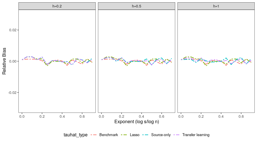
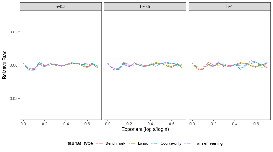
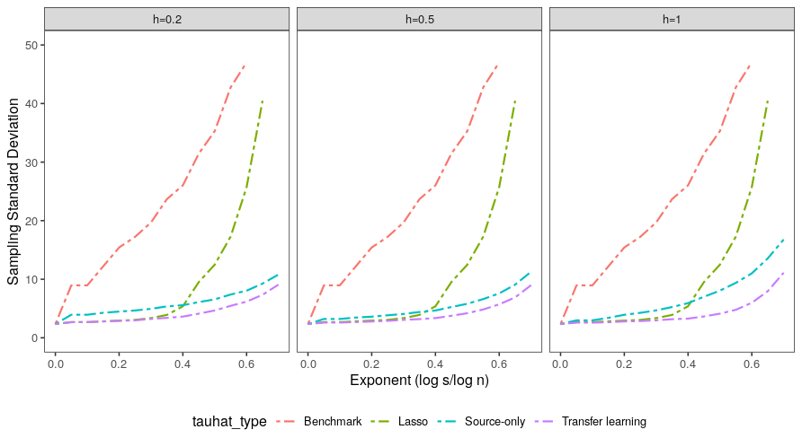
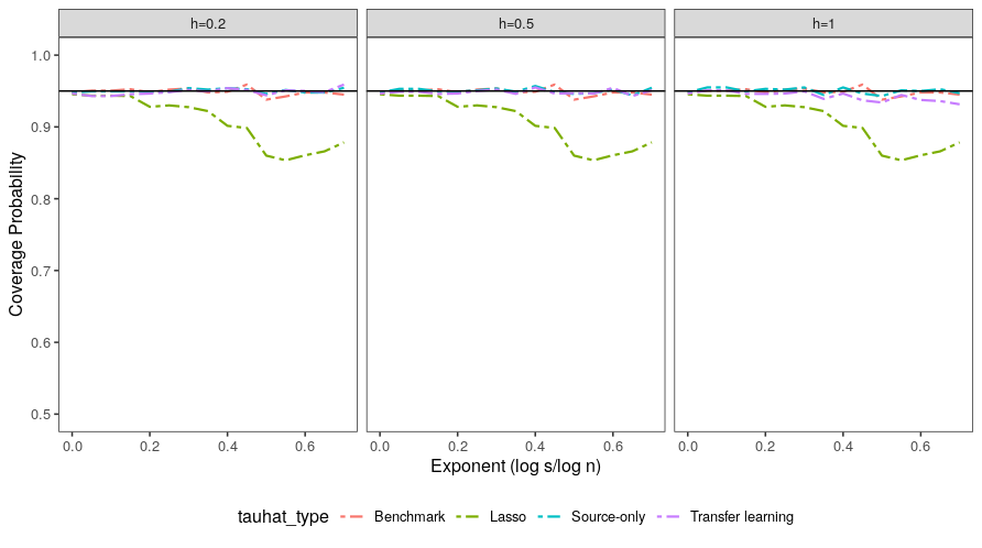
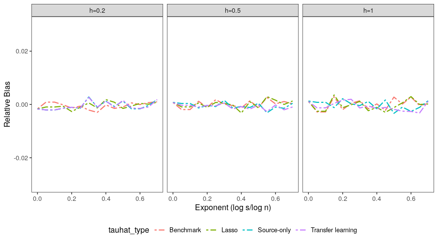
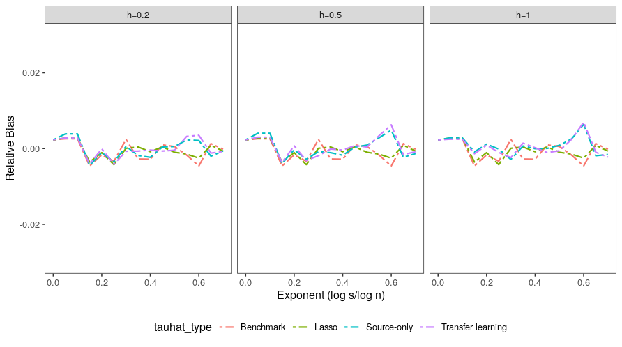
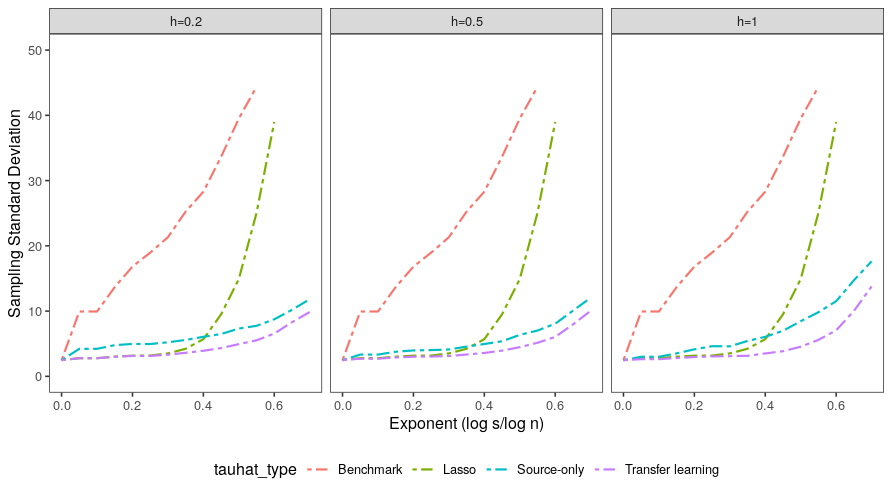
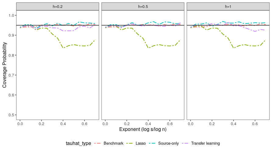
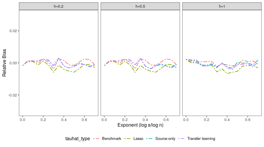
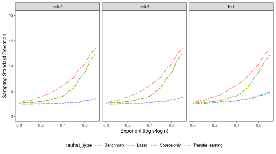
We represent the simulation results for four treatment effect estimators under stratified block randomization. The target data size is and the source data size is . The allocation ratio is 1:1:1 among treatments, with a block size of 6. Our estimators are calculated in replicates. The performances are measured by relative bias, standard deviation, and coverage probability of 95% confidence interval. The relative bias is defined as , where denotes any of our treatment effect estimators in the th replicate, is the true value of treatment effect, and is the sampling standard deviation. An additional result for unequal allocation ratio, which is 1:1:1 in the first strata and 2:2:1 in another strata, is in the Appendix. The results are summarized as follows:
-
•
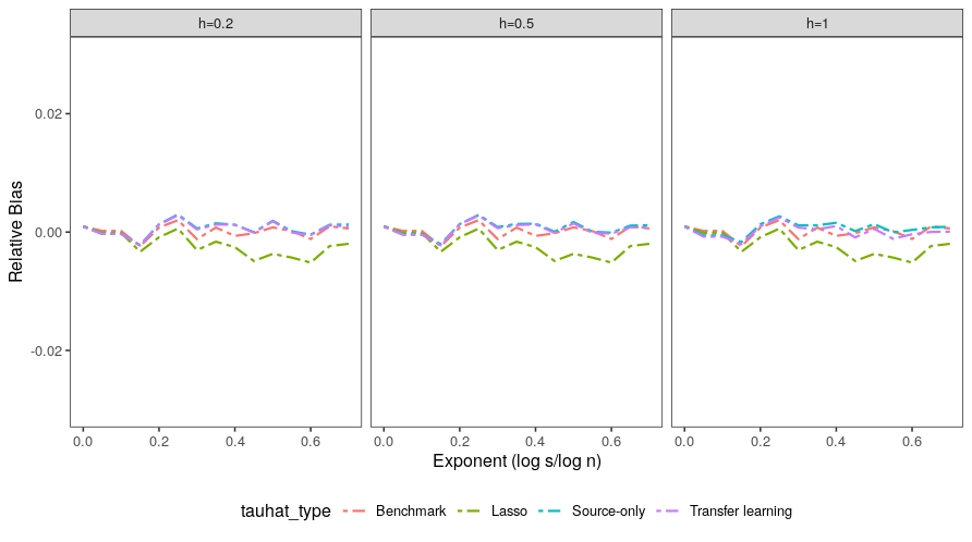
For all cases, the relative bias for all estimators is close to 0.
-
•
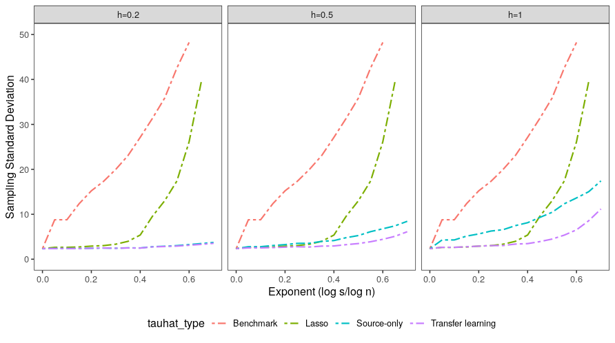
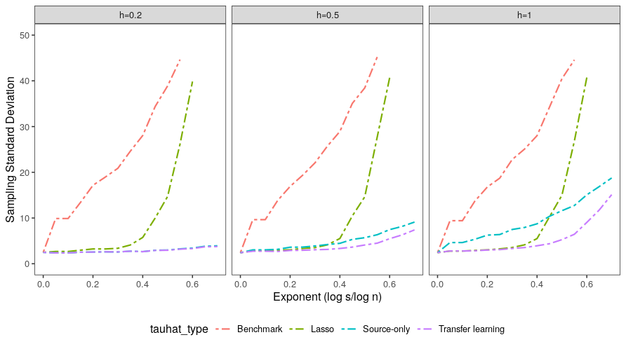
In Figure 1(b), the sampling standard deviation (SD) for all estimators increases when increases. When increases, the difference in the sampling standard deviation between and increases as the source data becomes far away from the target data. The difference can be eased by our transfer learning approach. As we expected, when is small, the sampling standard deviation for is similar to , which verifies Theorem 2; when is sufficient large, shows an efficiency gain compared to .
-
•
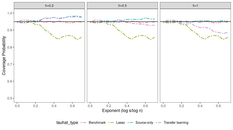
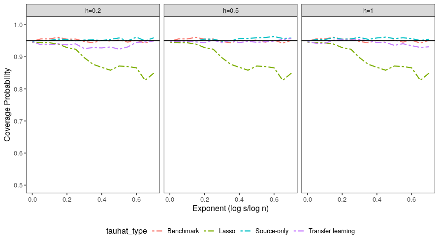
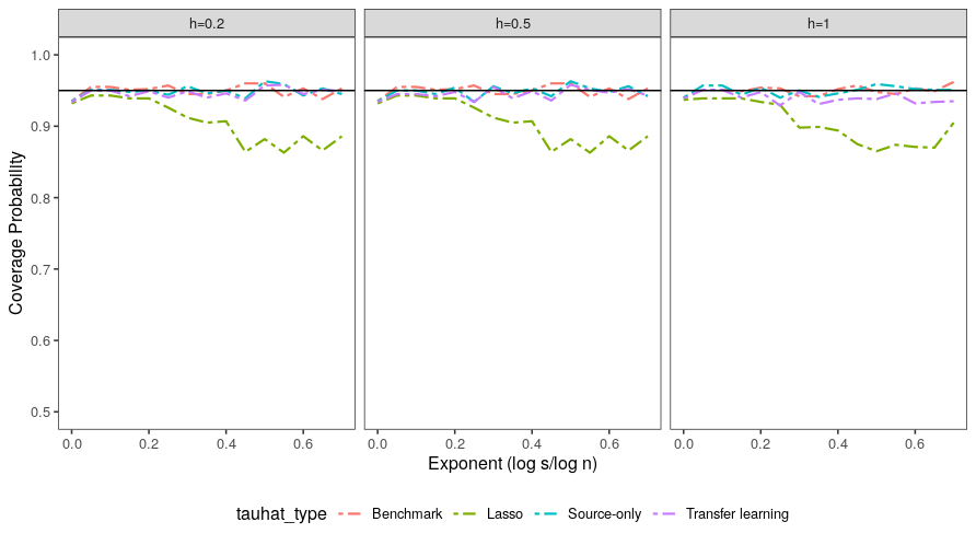
In Figure 1(c), shows an incredible decrease in coverage probability when increases, which may be caused by the overfitting when the condition () is violated, leading to an inconsistent variance estimator. As we have mentioned in Remark 5, the coverage probability is approximately 95% for . For , the estimation is conservative when . When and increases, maintains a 95% coverage probability as the conditions in Theorem 2 hold. Moreover, even when the condition is violated at , shows a slower decrease in coverage probability compared to .
-
•
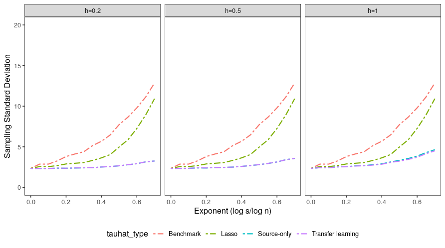
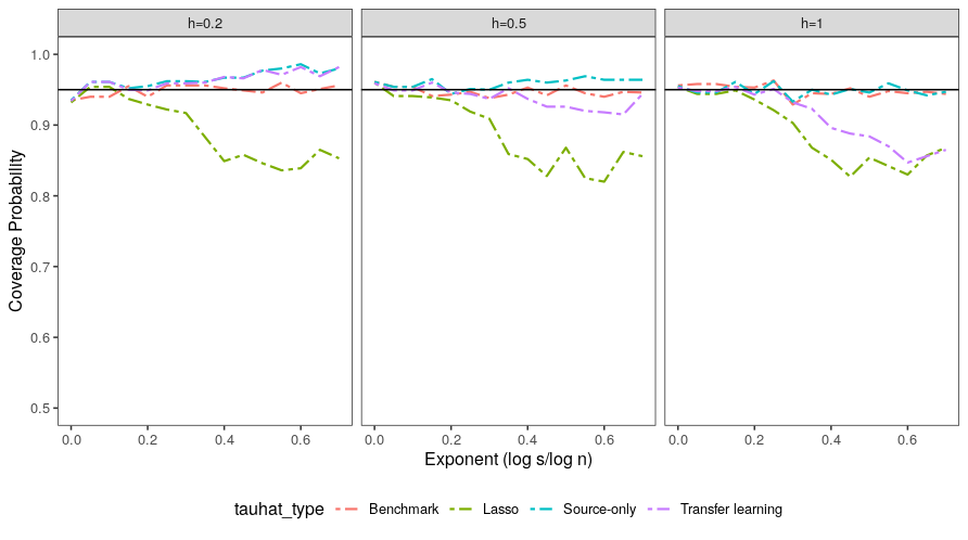
In Figures 2 and 3, the underlying model is misspecified from the linear model for source data or target data, respectively. The results for all measures are consistent with those presented in Figure 1, which shows that our transfer learning algorithm is robust regardless of whether the target data or the source data is misspecified. Especially our transfer learning approach performs better in Cases 2 and 3, with the coverage probabilities around 95%. This confirms that our proposed approach can provide valid inference when conditions are satisfied.
7 Clinical trial example
In this section, we consider an example of a clinical trial solely to generate synthetic data to illustrate the capability of our proposed estimators to improve efficiency compared with the benchmark and provide valid inference. We use synthetic data from a trial using nefazodone and the cognitive behavioral-analysis system of psychotherapy (CBASP) [Keller et al., 2000]. The trial aimed to compare the efficacy of nefazodone, CBASP, and their combination in the treatment of chronic depression. We consider the combination as the control group indexed as 0, nefazodone as the treatment indexed as 1, and the CBASP as the treatment indexed as 2. The outcome of interest was FinalHAMD, the final score of the 24-item Hamilton rating scale for depression. To generate the synthetic data, we first fit the data with a nonparametric spline using the function bigssa from the R package bigspline. Similar to Liu et al. [2023], we stratify the data using GENDER and select eight covariates to fit the model: AGE, HAMA SOMATI, HAMD17, HAMD24, HAMD COGIN, Mstatus2, NDE and TreatPD, which are detailed in Table 1. We take linear, quadratic, cubic, and interaction terms for continuous covariates, linear and interaction terms for binary covariates, and interaction terms for the above two sets of coordinates as the covariates resulting in for treatment effect estimators other than the benchmark estimator.
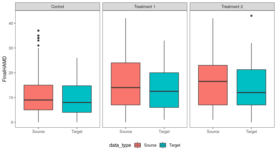
To generate the source and target data, we divide the data by HAMD17 such that the target population has HAMD17 less than 18 and the source population has HAMD17 greater than or equal to 18. The purpose is to create a difference in outcomes between the source and target data, as shown by a boxplot in Figure 4. Then, we sample 300 units among the target population with replacement as the target dataset. Similarly, we sample 1200 units from the source population with replacement as the source data. Next, we implement stratified block randomization on both the source and target data, using GENDER as the stratified variable with an allocation ratio of 1:1:1 for treatments and a block size of 6. We compare the performance of four estimators in Section 6. The treatment effects and variances are evaluated based on 1000 replicates. The coverage probabilities of the 95% confidence interval are assessed based on the estimates and variance estimators. The results are shown in Table 2.
As shown in Table 2, the treatment effect estimation for all four estimators is similar with positive results. The source-only estimator has the worst performance in terms of efficiency, which may decrease the efficiency compared with the benchmark estimator (variance reduction: -35.08%). Both and show efficiency gains compared with as the variance reduction range from 25.53% to 40.19%, and also shows an efficiency gain compared with . Moreover, and have better performance on coverage probabilities than , which are closer to 95%.
| Variable | Description |
|---|---|
| AGE | Age of patients in years |
| GENDER | 1 female and 0 male |
| HAMA_SOMATI | HAMA somatic anxiety score |
| HAMD17 | Total HAMD-17 score |
| HAMD24 | Total HAMD-24 score |
| HAMD_COGIN | HAMD cognitive disturbance score |
| Mstatus2 | Marriage status: 1 if married or living with someone and |
| 0 otherwise | |
| NDE | Number of depressive episodes |
| TreatPD | Treated past depression: 1 yes and 0 no |
| Note: HAMD, Hamilton Depression Scale; HAMA, Hamilton Anxiety Scale. | |
| Estimator | Estimate | Variance () | VR (%) | CP | Estimate | Variance () | VR (%) | CP |
|---|---|---|---|---|---|---|---|---|
| 4.46 | 15.97 | — | 0.956 | 4.29 | 22.7 | — | 0.954 | |
| 4.44 | 21.57 | -35.08 | 0.950 | 4.30 | 19.13 | 15.75 | 0.954 | |
| 4.46 | 11.89 | 25.53 | 0.933 | 4.30 | 15.38 | 32.25 | 0.913 | |
| 4.46 | 11.28 | 29.36 | 0.944 | 4.29 | 13.58 | 40.19 | 0.950 | |
| Note: CI, confidence interval; VR, variance reduction; CP, coverage probability | ||||||||
8 Discussion
In this paper, we incorporate external trial data into the inference under covariate-adaptive randomization by transfer learning. We first generalize the lasso-adjusted stratum-specific treatment effect estimator under multiple treatments. Then, we apply a transfer learning approach to develop the transfer learning estimator. The theoretical results show that our proposed estimator can enhance the lasso-adjusted stratum-specific estimator to have faster convergence rate of regression coefficient estimators and weaken the requirements on the sample size for asymptotic normality, when the source data and target data are similar under mild conditions. We also proposed a consistent variance estimator to provide valid inference. The simulation results and a clinical trial example confirm our findings. By proposing an effective transfer algorithm, offering theoretical guarantees, and developing a robust inference method, our study sheds light on the potential of transfer learning in analyzing randomized clinical trials.
Our transfer learning approach requires that the source data and target data are similar concerning the norm of the difference in regression coefficients. In practice, the external trial data may substantially differ from the current trial data. Consequently, selecting units from the external trial data that align with the current trial is crucial but may complicate inference due to the correlated selection procedure across both datasets. Therefore, identifying similar parts is a potential future work for our research. Meanwhile, the efficiency gain of the treatment effect estimation can be improved by estimating the underlying model between the response and the baseline covariates [Tu et al., 2023]. A potential improvement for our work is to replace the linear model with a general function for covariates. In this setting, future works may focus on characterizing the difference between the source data and the target data and proposing a proper transfer learning approach to develop a robust treatment effect estimator and ensure valid inference. Moreover, potential works can focus on adapting transfer learning to estimate other types of treatment effects, such as quantile treatment effects and interaction effects.
References
- Atkinson [1982] A. C. Atkinson. Optimum biased coin designs for sequential clinical trials with prognostic factors. Biometrika, 69:61–67, 1982.
- Bannick et al. [2023] M. S. Bannick, J. Shao, J. Liu, Y. Du, Y. Yi, and T. Ye. A general form of covariate adjustment in randomized clinical trials. arXiv preprint arXiv:2306.10213, 2023.
- Begg and Iglewicz [1980] C. B. Begg and B. Iglewicz. A treatment allocation procedure for sequential clinical trials. Biometrics, 36(1):81–90, 1980.
- Bugni et al. [2018] F. A. Bugni, I. A. Canay, and A. M. Shaikh. Inference under covariate-adaptive randomization. Journal of the American Statistical Association, 113(524):1784–1796, 2018.
- Bugni et al. [2019] F. A. Bugni, I. A. Canay, and A. M. Shaikh. Inference under covariate-adaptive randomization with multiple treatments. Quantitative Economics, 10(4):1747–1785, 2019.
- Cai et al. [2024] C. Cai, T. T. Cai, and H. Li. Transfer learning for contextual multi-armed bandits. The Annals of Statistics, 52(1):207–232, 2024.
- Cai and Pu [2024] T. T. Cai and H. Pu. Transfer learning for nonparametric regression: Non-asymptotic minimax analysis and adaptive procedure. arXiv preprint arXiv:2401.12272, 2024.
- Cai and Wei [2021] T. T. Cai and H. Wei. Transfer learning for nonparametric classification: Minimax rate and adaptive classifier. The Annals of Statistics, 49(1):100–128, 2021.
- Chevret et al. [2022] S. Chevret, J.-F. Timsit, and L. Biard. Challenges of using external data in clinical trials- an illustration in patients with COVID-19. BMC Medical Research Methodology, 22(1):321, 2022.
- Chu et al. [2023] J. Chu, W. Lu, and S. Yang. Targeted optimal treatment regime learning using summary statistics. Biometrika, 110(4):913–931, 2023.
- Ciolino et al. [2019] J. D. Ciolino, H. L. Palac, A. Yang, M. Vaca, and H. M. Belli. Ideal vs. real: A systematic review on handling covariates in randomized controlled trials. BMC Medical Research Methodology, 19:136–146, 2019.
- Colnet et al. [2024] B. Colnet, I. Mayer, G. Chen, A. Dieng, R. Li, G. Varoquaux, J.-P. Vert, J. Josse, and S. Yang. Causal inference methods for combining randomized trials and observational studies: A review. Statistical Science, 39(1):165–191, 2024.
- Dahabreh et al. [2020] I. J. Dahabreh, S. E. Robertson, J. A. Steingrimsson, E. A. Stuart, and M. A. Hernan. Extending inferences from a randomized trial to a new target population. Statistics in Medicine, 39(14):1999–2014, 2020.
- Donahue et al. [2014] J. Donahue, Y. Jia, O. Vinyals, J. Hoffman, N. Zhang, E. Tzeng, and T. Darrell. Decaf: A deep convolutional activation feature for generic visual recognition. In International conference on machine learning, pages 647–655. PMLR, 2014.
- Efron [1971] B. Efron. Forcing a sequential experiment to be balanced. Biometrika, 58(3):403–417, 1971.
- FDA [2022] FDA. Rare diseases: Natural history studies for drug development: Draft guidance for industry., 2022. URL https://www.fda.gov/media/122425/download.
- Freedman [2008] D. A. Freedman. On regression adjustments to experimental data. Advances in Applied Mathematics, 40(2):180–193, 2008.
- Gu et al. [2023] Y. Gu, H. Liu, and W. Ma. Regression-based multiple treatment effect estimation under covariate-adaptive randomization. Biometrics, 79(4):2869–2880, 2023.
- Hobbs et al. [2011] B. P. Hobbs, B. P. Carlin, S. J. Mandrekar, and D. J. Sargent. Hierarchical commensurate and power prior models for adaptive incorporation of historical information in clinical trials. Biometrics, 67(3):1047–1056, 2011.
- Hu and Zhang [2020] F. Hu and L.-X. Zhang. On the theory of covariate-adaptive designs. arXiv preprint arXiv:2004.02994, 2020.
- Hu et al. [2023] F. Hu, X. Ye, and L.-X. Zhang. Multi-arm covariate-adaptive randomization. Science China Mathematics, 66(1):163–190, 2023.
- Hu and Hu [2012] Y. Hu and F. Hu. Asymptotic properties of covariate-adaptive randomization. Annals of Statistics, 40(3):1794–1815, 2012.
- Huang et al. [2022] J. Huang, M. Wang, and Y. Wu. Estimation and inference for transfer learning with high-dimensional quantile regression. arXiv preprint arXiv:2211.14578, 2022.
- Ibrahim and Chen [2000] J. G. Ibrahim and M.-H. Chen. Power prior distributions for regression models. Statistical Science, pages 46–60, 2000.
- Ibrahim et al. [2015] J. G. Ibrahim, M.-H. Chen, Y. Gwon, and F. Chen. The power prior: theory and applications. Statistics in Medicine, 34:3724–3749, 2015.
- Jin et al. [2024] J. Jin, J. Yan, R. H. Aseltine, and K. Chen. Transfer learning with large-scale quantile regression. Technometrics, pages 1–30, 2024.
- Kallus et al. [2018] N. Kallus, A. M. Puli, and U. Shalit. Removing hidden confounding by experimental grounding. Advances in Neural Information Processing Systems, 31, 2018.
- Keller et al. [2000] M. B. Keller, J. P. McCullough, D. N. Klein, B. Arnow, D. L. Dunner, A. J. Gelenberg, J. C. Markowitz, C. B. Nemeroff, J. M. Russell, M. E. Thase, et al. A comparison of nefazodone, the cognitive behavioral-analysis system of psychotherapy, and their combination for the treatment of chronic depression. New England Journal of Medicine, 342(20):1462–1470, 2000.
- Lee et al. [2023] D. Lee, S. Yang, L. Dong, X. Wang, D. Zeng, and J. Cai. Improving trial generalizability using observational studies. Biometrics, 79(2):1213–1225, 2023.
- Li et al. [2022] S. Li, T. T. Cai, and H. Li. Transfer learning for high‐dimensional linear regression: Prediction, estimation and minimax optimality. Journal of the Royal Statistical Society Series B, 84(1):149–173, 2022.
- Li et al. [2023] S. Li, T. T. Cai, and H. Li. Transfer learning in large-scale gaussian graphical models with false discovery rate control. Journal of the American Statistical Association, 118(543):2171–2183, 2023.
- Lin [2013] W. Lin. Agnostic notes on regression adjustments to experimental data: Reexamining freedman’s critique. The Annals of Applied Statistics, 7(1):295–318, 2013.
- Liu et al. [2023] H. Liu, F. Tu, and W. Ma. Lasso-adjusted treatment effect estimation under covariate-adaptive randomization. Biometrika, 110(2):431–447, 2023.
- Ma et al. [2022] W. Ma, F. Tu, and H. Liu. Regression analysis for covariate-adaptive randomization: A robust and efficient inference perspective. Statistics in Medicine, 41(29):5645–5661, 2022.
- Negahban et al. [2009] S. N. Negahban, P. Ravikumar, M. J. Wainwright, and B. Yu. A unified framework for high-dimensional analysis of m-estimators with decomposable regularizers. Advances in Neural Information Processing Systems, 22, 2009.
- Neuenschwander et al. [2010] B. Neuenschwander, G. Capkun-Niggli, M. Branson, and D. J. Spiegelhalter. Summarizing historical information on controls in clinical trials. Clinical Trials, 7(1):5–18, 2010.
- Neyman [1923] J. S. Neyman. On the application of probability theory to agricultural experiments. essay on principles. section 9. Annals of Agricultural Sciences, 10:1–51, 1923.
- Pan and Yang [2009] S. J. Pan and Q. Yang. A survey on transfer learning. IEEE Transactions on Knowledge and Data Engineering, 22(10):1345–1359, 2009.
- Petegrosso et al. [2017] R. Petegrosso, S. Park, T. H. Hwang, and R. Kuang. Transfer learning across ontologies for phenome–genome association prediction. Bioinformatics, 33(4):529–536, 2017.
- Pocock [1976] S. J. Pocock. The combination of randomized and historical controls in clinical trials. Journal of Chronic Diseases, 29(3):175–188, 1976.
- Pocock and Simon [1975] S. J. Pocock and R. Simon. Sequential treatment assignment with balancing for prognostic factors in the controlled clinical trial. Biometrics, 31(1):103–115, 1975.
- Rafi [2023] A. Rafi. Efficient semiparametric estimation of average treatment effects under covariate adaptive randomization. arXiv preprint arXiv:2305.08340, 2023.
- Rosenberger and Lachin [2015] W. F. Rosenberger and J. M. Lachin. Randomization in Clinical Trials: Theory and Practice. John Wiley & Sons, 2nd edition, 2015.
- Rubin [1974] D. B. Rubin. Estimating causal effects of treatments in randomized and nonrandomized studies. Journal of Educational Psychology, 66(688), 1974.
- Ruder et al. [2019] S. Ruder, M. E. Peters, S. Swayamdipta, and T. Wolf. Transfer learning in natural language processing. In Proceedings of the 2019 conference of the North American chapter of the association for computational linguistics: Tutorials, pages 15–18, 2019.
- Saenko et al. [2010] K. Saenko, B. Kulis, M. Fritz, and T. Darrell. Adapting visual category models to new domains. In European conference on computer vision, pages 213–226. Springer, 2010.
- Schmidli et al. [2014] H. Schmidli, S. Gsteiger, S. Roychoudhury, A. O’Hagan, D. Spiegelhalter, and B. Neuenschwander. Robust meta-analytic-predictive priors in clinical trials with historical control information. Biometrics, 70(4):1023–1032, 2014.
- Schweikert et al. [2008] G. Schweikert, G. Rätsch, C. Widmer, and B. Schölkopf. An empirical analysis of domain adaptation algorithms for genomic sequence analysis. Advances in Neural Information Processing Systems, 21, 2008.
- Shao et al. [2010] J. Shao, X. Yu, and B. Zhong. A theory for testing hypotheses under covariate-adaptive randomization. Biometrika, 97(2):347–360, 2010.
- Stuart et al. [2011] E. A. Stuart, S. R. Cole, C. P. Bradshaw, and P. J. Leaf. The use of propensity scores to assess the generalizability of results from randomized trials. Journal of the Royal Statistical Society Series A: Statistics in Society, 174(2):369–386, 2011.
- Taves [1974] D. R. Taves. Minimization: A new method of assigning patients to treatment and control groups. Clinical Pharmacology & Therapeutics, 15(5):443–453, 1974.
- Tian and Feng [2023] Y. Tian and Y. Feng. Transfer learning under high-dimensional generalized linear models. Journal of the American Statistical Association, 118(544):2684–2697, 2023.
- Tibshirani [1996] R. Tibshirani. Regression shrinkage and selection via the lasso. Journal of the Royal Statistical Society: Series B (Methodological), 58(1):267–288, 1996.
- Torrey and Shavlik [2010] L. Torrey and J. Shavlik. Transfer learning. In Handbook of Research on Machine Learning Applications and Trends: Algorithms, Methods, and Techniques, pages 242–264. IGI global, 2010.
- Tu et al. [2023] F. Tu, W. Ma, and H. Liu. A unified framework for covariate adjustment under stratified randomization. arXiv preprint arXiv:2312.01266, 2023.
- Wah et al. [2011] C. Wah, S. Branson, P. Welinder, P. Perona, and S. Belongie. The caltech-ucsd birds-200-2011 dataset. 2011.
- Weiss et al. [2016] K. Weiss, T. M. Khoshgoftaar, and D. Wang. A survey of transfer learning. Journal of Big Data, 3(1):1–40, 2016.
- Wolf et al. [2020] T. Wolf, L. Debut, V. Sanh, J. Chaumond, C. Delangue, A. Moi, P. Cistac, T. Rault, R. Louf, M. Funtowicz, et al. Transformers: State-of-the-art natural language processing. In Proceedings of the 2020 conference on empirical methods in natural language processing: system demonstrations, pages 38–45, 2020.
- Wu and Yang [2022] L. Wu and S. Yang. Integrative -learner of heterogeneous treatment effects combining experimental and observational studies. In Conference on Causal Learning and Reasoning, pages 904–926. PMLR, 2022.
- Wu and Yang [2023] L. Wu and S. Yang. Transfer learning of individualized treatment rules from experimental to real-world data. Journal of Computational and Graphical Statistics, 32(3):1036–1045, 2023.
- Yang et al. [2020] F. Yang, H. R. Zhang, S. Wu, W. J. Su, and C. Ré. Analysis of information transfer from heterogeneous sources via precise high-dimensional asymptotics. arXiv preprint arXiv:2010.11750, 2020.
- Yang and Tsiatis [2001] L. Yang and A. A. Tsiatis. Efficiency study of estimators for a treatment effect in a pretest–posttest trial. The American Statistician, 55(4):314–321, 2001.
- Yang et al. [2023] S. Yang, C. Gao, D. Zeng, and X. Wang. Elastic integrative analysis of randomised trial and real-world data for treatment heterogeneity estimation. Journal of the Royal Statistical Society Series B: Statistical Methodology, 85(3):575–596, 2023.
- Ye et al. [2022] T. Ye, Y. Yi, and J. Shao. Inference on the average treatment effect under minimization and other covariate-adaptive randomization methods. Biometrika, 109:33–47, 2 2022.
- Ye et al. [2023] T. Ye, J. Shao, Y. Yi, and Q. Zhao. Toward better practice of covariate adjustment in analyzing randomized clinical trials. Journal of the American Statistical Association, 118(544):2370–2382, 2023.
- Zelen [1974] M. Zelen. The randomization and stratification of patients to clinical trials. Journal of Chronic Diseases, 27(7):365–375, 1974.
- Zhang and Zhang [2014] C.-H. Zhang and S. S. Zhang. Confidence intervals for low dimensional parameters in high dimensional linear models. Journal of the Royal Statistical Society Series B: Statistical Methodology, 76(1):217–242, 2014.
- Zhuang et al. [2020] F. Zhuang, Z. Qi, K. Duan, D. Xi, Y. Zhu, H. Zhu, H. Xiong, and Q. He. A comprehensive survey on transfer learning. Proceedings of the IEEE, 109(1):43–76, 2020.
Appendix
Appendix A General theory for regression adjustment under covariate-adaptive randomization with multiple treatments
We develop a general theory for regression-adjusted treatment effect estimators, which we can apply to the lasso-adjusted and transfer learning estimators.
Assumption A.1.
For and , there exists coefficient vectors such that
Remark A.1.
We develop the asymptotic normality by first deriving the asymptotic normality for the potential outcomes and then using linear transformation to obtain the result, where for . Therefore, Assumption A.1 is the remaining term for the first step and needs to be .
Remark A.2.
When the dimension is fixed, by Bugni et al. [2018]. Therefore, when element-wisely converges to , Assumption A.1 holds. Remark 2 in Gu et al. [2023] also explained this result when using the stratum-common estimator. However, the OLS estimator may not satisfy this condition when is diverging or even larger than the sample size.
Let be a general estimator for treatment effect .
and
Also, we define the transformed outcome , for .
Proposition A.1.
Proof.
The asymptotic normality can be derived from Theorem 2 in Gu et al. [2023] under Assumption A.1 with minor changes. Recall that
Then we have
The proof falls to show that the first two terms are asymptotic normal and the last term is . By Assumption 4, we have
for all . As the stratum size is finite, we have
for all .
Then we show that the first two terms are asymptotic normal. Simple calculation shows that
Define
Here is a transformed outcome, and
In Bugni et al. [2019], it takes . Some calculation for the first two parts of leads to
where and . By Lemma 1 and some additional calculations, we have
where
Let , we have
∎
Appendix B Proof of main theorems
B.1 Proof of Proposition 1
Proof.
By the definition of Lasso estimator, we have
Therefore, we have
Let . Let , for , be a transformed outcome. Here means the units such that . Also, we denote
Then by some calculations,
By Lemma 3, it has high probability that
Therefore, we have
As is the union of the support of for , we have
Therefore, we split the norm into the parts in and , and by triangle inequality:
we have
As all three terms are greater than or equal to zero, we have . Let
where . By Lemma 4,
Under , we have
That is
Then
Therefore, as , we have
Then by Lemma 2, , we have
The last line is due to Assumption 4. The assumptions for Proposition A.1 hold, so we have
In Proposition A.1, when for , we have
Therefore, the asymptotic covariance matrix is where ∎
B.2 Proof of Theorem 1
Proof.
Transfer Step.
By the definition of , we have
Let . By some calculations, we have
where
Here , for .
Let . By Lemma 3, we have
Then under ,
Recall that and is the complementary set of . Let and for any vector . We split and apart and take following inequalities:
Then we have
Then we compare the first term and the second term on the RHS.
Case 2 :
Then
A direct bound for is
The third inequality holds as
Also, by RSC condition and Lemma 5, we have
Under condition that , we have
This is used for the proof in the debiasing step. Therefore, we have
Debiasing Step:
Let . By similar calculations in the Transfer step, we have
Recall that , as
we have
Here and are the same as the ones defined in the Proof of Proposition 1. We focus on the third term on the RHS first. By triangle inequality and basic inequality , we have
Let
By Lemma 3 we have
Therefore, under , we have
As
we have
Case 1:
We have
Case 2:
We have
The second inequality holds as is uniformly bounded and
In the Transfer Step, we already have
Therefore,
By Assumptions 4 and 7, we have
We assume that is the same and consider the convergence of the subsequence. We can require that is monotonically increasing but is decreasing when is large enough. can diverge slowly to satisfy our conditions, such as . Then
when and are large enough. Therefore,
According to the inequalities for and , in high probability that we have
for some constant and independent with and . When , we can write the above term as
∎
B.3 Proof of Theorem 2
B.4 Proof of Theorem 3
B.5 Lemmas with proof
Proof.
Most of the proof is similar to the proof for Lemma 5 in Gu et al. [2023]. The difference is that in this Lemma, may not be as we define in the context. The consequence is that for most cases. The remaining parts are the same and we omit the proof. ∎
Proof.
The proof is similar to the proof of Lemma S4 in Liu et al. [2023]. We can replace into for all to show our result. Therefore, we omit the proof. ∎
Lemma 3.
Proof.
The proof is similar to the proof of Lemma S5 in Liu et al. [2023]. It’s a special case for stratum size . At the same time, we can replace into for all to show our result. Therefore, we omit the proof. ∎
Lemma 4.
Proof.
We use a similar argument in Bugni et al. [2018]. As are i.i.d. data and is independent with conditional on . Therefore, given the and , the distribution of is the same if we order the units first by strata and then by treatments within each strata. Then, independently with and , let has the same distribution with given . Then has the same distribution with
By Assumption 1, is uniformly bounded by a constant . As has the same distribution with given , is uniformly bounded by constant so that is a sub-Gaussian random vector. According to Proposition 2 in Negahban et al. [2009] for generalized linear models, it can be applied directly to the standard linear model. For any , we have
with probability at least . Here only depends on the minimum eigenvalue of covariance matrix and .
As we can divide on both sides, we have
Next, we consider the vectors in the convex cone
For any vector ,
Therefore,
Under Assumption , we have
when . Therefore,
| (1) |
when . Using the almost sure representation theorem, we can construct (independent of ) such that has the same distribution with and almost surely. Therefore, for any ,
where the convergence follows from the dominant convergence theorem, a.s., independence of and and (1). Therefore
∎
Proof.
Similar to the proof of Lemma 4, we construct and has the same distribution with
Also, by the same argument in Negahban et al. [2009], when ,
By a general inequality, we have
for some positive constant . We can choose , then we have
for some positive constant and . Then by the similar arguments in the proof of Lemma 4, we have
∎
Lemma 6.
Under conditions in Proposition A.1, suppose there exist and , such that
for all . Let be the estimator of , such that
Then we have
is a consistent estimator for .
Proof.
The proof of the consistency of the variance estimator is similar to the proof of Theorem 3 in Gu et al. [2023]. The proof for stays the same. We will focus on and the other two terms.
The consistency of the estimator can be implied by
for and , and
By Lemma 7 below, we have
Then we have
The third term converges to zero due to the condition that
and the second term converges to zero due to the Cauchy-Schwarz inequality. Similarly, in the last term of the variance estimator, we can only deal with
Also, it is sufficient to show that for any treatment and , we have
The left-hand side can be expressed as
As
and the second term is due to the Cauchy-Schwarz inequality, we show the convergence of the last term in the estimator.
Finally, we need to show that
We can write the LHS as
and split the term into three parts:
and their production. Similar to the former arguments, the first term converges to the result. The second term converges to zero due to the condition and the Cauchy-Schwarz inequality. ∎
Lemma 7.
For which satisfies , we have
Appendix C Additional simulations
Figures A1–A3 represent the simulation results when the allocation ratios are unequal within each stratum in the main text. The allocation ratios are 1:1:1 in the first strata and 2:2:1 in the other strata, and the block size for the stratified block randomization is 15. Other settings are the same as the settings in Section 6 in the main text. The simulation results are similar to the results in the main text.