Stochastic Scovil–Schulz-DuBois machine

Abstract

Three types of cycles are identified in the quantum jump trajectories of the Scovil–Schulz-DuBois (SSDB) machine: an R-cycle as refrigeration, an H-cycle as a heat engine, and an N-cycle in which the machine is neutral. The statistics of these cycles are investigated via a semi-Markov process method. We find that in the large time limit, whether the machine operates as a heat engine or refrigerator depends on a balance between the numbers of R-cycles and H-cycles per unit time. Further increasing the hot bath temperature above a certain threshold does not increase the machine’s power output. The cause is that, in this situation, the N-cycle has a greater probability than the H-cycle and R-cycle. Although the SSDB machine operates by randomly switching among these three cycles, at the level of a single quantum jump trajectory, its heat engine efficiency and the refrigerator’s coefficient of performance remain constant.

I Introduction

The Scovil and Schulz-DuBois (SSDB) quantum heat engine [1] is the cornerstone of quantum thermodynamics [2]. Since it was first proposed in 1959, the notion of quantum thermal machines has attracted considerable theoretical and experimental interest [3, 4, 5, 6, 7, 8, 9, 10, 11, 12, 13, 14, 15, 16, 17, 18, 19, 2, 20, 21, 22, 23].

Although many quantum thermal machines have been proposed, owing to their simplicity and rich physics, SSDB machines continue to be investigated from various aspects  [8, 13, 24, 25, 26, 27, 28]. Figure (1)(a) schematically shows the machine. This system comprises a three-level atom and two heat baths with temperatures $T_{1}$ and $T_{2}$, where $T_{1}>T_{2}$. The atom is also weakly driven by a classically resonant single-mode field. Given that the foundation of the machine is quantum physics, it essentially operates randomly and probabilistically. Earlier studies focused on the average behaviors or characteristics of the machine at the ensemble level [29, 30, 13]. Nevertheless, following the rapid development of stochastic thermodynamics [31, 32, 33, 34, 35, 36], many efforts have been devoted to machine randomness [25, 24, 27, 28]. For example, Menczel et al. [28] and Kalaee et al. [27] applied full counting statistics (FCS) to investigate violations of the thermodynamic uncertainty relation [37, 38] in the quantum machine.

This paper arises from a simple question: Does the SSDB machine operate cyclically similar to classical thermal machines? Analogizing the quantum thermal machine to the classical machine is not new. In fact, this analogy was first introduced in the original paper of Scovil and Schulz-DuBois. They wrote that “As any heat engine, this system should be reversible so that it acts as a refrigerator. This is indeed the case. Suppose a quantum $h\nu_{s}$ is applied to the signal transition. It causes an ion (the atom in this paper) to go from state 1 to 2. The ion may further jump to state 3 if energy $h\nu_{i}$ is supplied by the cold reservoir. The cycle is finally completed when the ion returns from state 3 to state 1 while the energy $h\nu_{p}$ is communicated to the hot reservoir. In this process, energy is extracted from the idler transition, that is, from the cold reservoir, so that it is refrigerated.”. Similar statements are also present in recent papers [25, 27]. This analogy is appealing because it provides an intuitive picture of the operation of the abstract quantum machine. However, it is also questionable. When we examine the previous statements, we do not see crucial terminologies of quantum physics, e.g., wave function, superposition, and coherence. Hence, the analogy fails to reveal crucial physics in the quantum regime. These authors did not implement this analogy in practical calculations and analysis.

In macroscopic thermodynamics, one cycle of a thermal machine is a thermodynamic process in which the system starts from an initial state and returns to the same initial state for the first time, e.g., the famous Carnot cycle of a heat engine or refrigerator. An often-overlooked fact is that the cycles are executed on a single machine. Following the previous analogy, we might infer that the cycles in the SSDB machine would be perceived at the single-atom level if the cycle notion is valid. In the literature, the SSDB machine is typically described via the quantum master equation (QME), which is related to the reduced density matrix of the atom [39, 40]. Hence, the theory is essentially an ensemble. In addition, it is well established that the QME can be unraveled into the quantum jump trajectory (QJT), a notion that is particularly relevant to the single-atom level  [41, 42, 43, 44, 45]. Therefore, in this work, we attempt to explore the cycle notion in the QJTs and investigate the statistics and thermodynamic meanings of cycles in the operation of the SSDB machine. Although thermodynamic interpretations of QJTs have been recognized for many years [46, 47, 48, 49, 50, 51], to our knowledge, few studies have directly examined quantum thermal machines from the QJT perspective [52, 53].

The remainder of this paper is organized as follows. In Sec. (II), we unravel the QME of the SSDB machine into the QJT. In Sec. (III), we decompose the QJT into a stochastic combination of three types of cycles. In Sec. (IV), using a semi-Markov process (SMP) method for open quantum systems, we investigate the means and fluctuation strengths of the cycle rates. Section (VI) concludes this paper.

II Unraveling the SSDB machine into a quantum jump trajectory

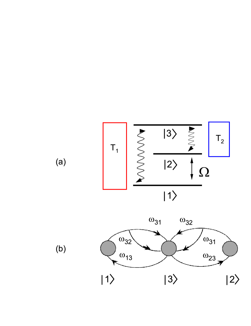
Figure 1: (a) Schematic of the SSDB machine. The line with double arrows represents a classically resonant single-mode driving field. The coupling strength of the field with the three-level atom is $\Omega$. The squares on the left and right represent the heat baths, with temperatures $T_{1}$ and $T_{2}$, respectively. (b) Schematic of the QJTs of the SSDB machine. The gray dots indicate the collapsed quantum states. They are also the states from which the wave functions start. Curves without arrows represent deterministic pieces of the wave functions, whereas those with arrows represent collapses of the wave functions. Note that these curves merge in the QJTs connecting $|3\rangle$ and $|1\rangle$ or $|2\rangle$. The symbols $\omega_{3i}=E_{3}-E_{i}$ and $\omega_{i3}=E_{i}-E_{3}$, $i=1,2$, near the arrows, denote the quanta exchanged between the atom and the $T_{i}$-heat bath, where $E_{i}$ and $E_{3}$ are the energy levels of the atom. These quanta are also interpreted as the heat absorbed by the atom from the heat baths. A negative value of $\omega_{i3}$ indicates that the $T_{i}$-heat bath absorbs heat from the atom.

In the rotation framework, the QME for the three-level atom is

$$\partial_{t}\rho = -{\rm i}\left[H,\rho(t)\right]+{\cal D}_{13}[\rho]+{\cal D}_{23}[\rho].$$ (1)

In this equation, $\rho$ is the reduced density matrix of the atom, the Planck constant $\hbar$ is set to 1, and the interaction Hamiltonian between the atom and the field is

$$H=-\frac{\Omega}{2}(\sigma_{12}+\sigma_{21}),$$ (2)

where $\Omega$ represents the Rabi frequency. We also assume that the field is resonant for simplicity in the calculations. Abandoning this assumption does not considerably change the main results in this paper. The action of the dissipated superoperator ${\cal D}_{i3}$, $i=1,2$, on the density matrix $\rho$ is as follows:

$${\cal D}_{i3}(\rho) = r_{i}^{-}\left[\sigma_{i3}\rho(t)\sigma_{3i}-\frac{1}{2}\{\sigma_{3i}\sigma_{i3},\rho(t)\}\right]$$ (3)

$$+ r_{i}^{+}\left[\sigma_{3i}\rho(t)\sigma_{i3}-\frac{1}{2}\{\sigma_{i3}\sigma_{3i},\rho(t)\}\right],$$

where $\sigma_{i3}=|i\rangle\langle 3|$ and $\sigma_{3i}=|3\rangle\langle i|$ are the jump operators; $r_{i}^{-}=r_{i}(n_{i}+1)$ and $r_{i}^{+}=r_{i}n_{i}$ are the damping and exciting rates of the atom due to coupling with the $T_{i}$-heat bath, respectively; and $r_{i}$ and $n_{i}$ are the spontaneous emission rate and the Bose–Einstein distribution of the $T_{i}$ heat bath, respectively.

Equation (1) can be unraveled into the QJTs of single atoms [41, 42, 54, 55, 56, 44, 45]. A QJT is composed of deterministic pieces and random collapses of wave functions. Figure (1)(b) shows this scenario: The gray dots represent the quantum states $|i\rangle$, $i=1,2,3$, the curves without arrows denote that the wave functions of the atom start from these states and continuously evolve, and the curves with arrows denote the random collapses of the wave functions into the states. From the perspective of a stochastic process, if only the collapse events of the wave functions are considered, which include the collapsed quantum states and collapse times, the QJTs can be considered realizations of a certain SMP [57]. Under this idea, the evolution of the wave functions is replaced with the waiting time distributions (WTDs) of the SMP. For the SSDB machine, the WTDs are formulated as

$$p^{(j)}_{3|i}(\tau) = r_{i}^{+}\left|\sigma_{3j}e^{-{\rm i}{\tilde{H}}\tau}|i\rangle\right|^{2},$$ (4)

$$p_{i|3}(\tau) = r_{i}^{-}\left|\sigma_{i3}e^{-{\rm i}{\tilde{H}}\tau}|3\rangle\right|^{2},$$ (5)

$i,j=1,2$, where

$$\tilde{H}=H-\frac{{\rm i}}{2}\sum_{i=1}^{2}r_{i}^{-}\sigma_{3i}\sigma_{3i}-\frac{{\rm i}}{2}\sum_{i=1}^{2}r_{i}^{+}\sigma_{i3}\sigma_{i3}$$ (6)

is the non-Hermitian Hamiltonian [44]. In Eq. (4), $p^{(j)}_{3|i}$ is the WTD in which the wave function starts from state $|i\rangle$, continuously evolves, and finally collapses to state $|j\rangle$ through the jump operator $\sigma_{3j}$ at age $\tau$. In Eq. (5), $p_{i|3}$ has a similar explanation except that the starting and collapsed states are $|3\rangle$ and $|i\rangle$, respectively. In the latter case, the jump operator is $\sigma_{i3}$. These formulas can be solved explicitly, and the expressions depend on the values of the physical parameters. Nevertheless, their Laplace transforms with respect to age $\tau$ do not. We reserve Appendix A for these results. Here, we emphasize that the WTDs $p_{i|j}$, $i,j=1,2$, are precisely zero. This result is determined by the special structure of the QME (1). Hence, the connections between the gray dots in Fig. (1)(b) are meaningful. This point is closely related to the operation of the SSDB machine.

III Three types of cycles

In this work, we are interested in the energy exchanges between the three-level atom and the heat baths in the large time limit. According to a thermodynamic interpretation of the QJTs, a collapse of the wave function indicates a discrete amount of heat or a quantum absorbed by the atom from one of the heat baths. The sign and magnitude of the heat are given by the jump operators in the QME (1) [46, 47, 48, 49, 50, 51]. We mark these quanta near the arrows in Fig. (1)(b). By simultaneously tracking the collapsed quantum states and the quanta, we may construct an energy “path” and define thermodynamic quantities in an arbitrary QJT. For example, let $\bf X$ be a trajectory; then, the heat absorbed by the atom from the $T_{1}$- and $T_{2}$-heat baths is equal to

$$Q_{1}[{\bf X}] = \omega_{31}\Delta m[{\bf X}],$$ (7)

$$Q_{2}[{\bf X}] = \omega_{32}\Delta n[{\bf X]},$$ (8)

respectively. Here, $\Delta m[\bf X]$ ($\Delta n[\bf X]$) denotes the net number of quanta $\omega_{31}$ ($\omega_{32}$) absorbed by the atom from the $T_{1}$- ($T_{2}$-) heat bath in the full trajectory, which is also equal to the number of quanta $\omega_{31}$ ($\omega_{32}$) minus the number of quanta $\omega_{13}$ ($\omega_{23}$). Because of the first law of thermodynamics, the work output in the QJT is

$$A[{\bf X}]=Q_{1}[{\bf X}]+Q_{2}[{\bf X}].$$ (9)

After carefully inspecting Fig. (1)(b), we notice that a QJT is a stochastic combination of cycles . Here, a cycle refers to a QJT that starts from state $|3\rangle$ and ends in the same state for the first time. Considering the accompanying quanta in these cycles, we further classify them into four types: N₁, R, H, and N₂. Figure (2)(a) presents their diagrammatic representations. Note that we depict these quantum states from left to right. The energy scenarios of these cycles are straightforward. Let $(m_{+},m_{-},n_{+},n_{-})$ be the number of quanta in a cycle, where $m_{+}$ and $m_{-}$ denote the numbers of quanta $\omega_{31}$ and $\omega_{13}$, respectively, and where $n_{+}$ and $n_{-}$ denote the numbers of quanta $\omega_{32}$ and $\omega_{23}$, respectively. Specifically, we have N₁ cycles, $(1,1,0,0)$; R cycles, $(0,1,1,0)$; H cycles, $(1,0,0,1)$; and N₂ cycles, $(0,0,1,1)$. We further define $\Delta m=m_{+}-m_{-}$ and $\Delta n=n_{+}-n_{-}$. These quantities actually correspond to $\Delta m[\bf X]$ and $\Delta n[\bf X]$ in Eqs. (7) and (8), respectively, except that the QJT here is only one of the cycles. We immediately observe that in any type of cycle, the identity

$$\Delta m=-\Delta n$$ (10)

holds. Equation (10) reminds us of a statement made by Mitchison [59]. He argued that there is a perfect cooperative transfer of precisely one quantum each from the cold heat bath into the hot one. Our identity (10) not only extends this statement to the context of cycles but also covers a reverse procedure and an overlooked case involving zero quantum transfer. If we apply Eqs. (9) and (10) to the cycles, the work output is

$$\omega_{31}\Delta m+\omega_{32}\Delta n=\omega_{21}\Delta m.$$ (11)

The physical importance of these four types of cycles is now apparent: The R-cycle indicates that the SSDB machine operates as a refrigerator by work input ($\Delta m=-1$); in the H-cycle, the machine operates as a heat engine by positive work output ($\Delta m=1$); and in the N₁- and N₂-cycles, the machine is idle or neutral ($\Delta m=0$). Owing to their identical vanishing operations, we refer to the N₁-cycle and the N₂-cycles as N-cycles for the remainder of this paper and do not discuss them separately.

Let us return to the arbitrary QJT $\bf X$. On the basis of the above discussion, we conclude that the SSDB machine operates randomly by switching among three distinct types of cycles. Figure (2)(b) shows an example. Accordingly, the thermodynamic quantities possess alternative expressions:

$$Q_{1}[{\bf X}] = \omega_{31}\sum_{I}\Delta m_{I},$$ (12)

$$Q_{2}[{\bf X}] = \omega_{32}\sum_{I}\Delta n_{I},$$ (13)

$$A[{\bf X}] = \omega_{21}\sum_{I}\Delta m_{I}.$$ (14)

Here, the subscript $I$ denotes the $I$-th cycle in the trajectory. Although the SSDB machine is stochastic, Eq. (9) implies that we can still define it as a heat engine or refrigerator if the work output is positive or negative in the large time limit. In this context, studying rates instead of time-extensive quantities is more convenient [60]. To this end, we define power ${\cal P}=A[{\bf X}]/t$ and the net number of quanta $\omega_{31}$ absorbed by the atom from the $T_{1}$-heat bath per unit time,

$${\cal M}=\frac{\Delta m[{\bf X}]}{t}=\frac{\sum_{I}\Delta m_{I}}{t}.$$ (15)

These two quantities are random variables that are proportional to each other. In addition, because $\Delta m_{I}$ is equal to $-1$ and $+1$ for the R-cycle and H-cycle, respectively, $\cal M$ has a further expression:

$${\cal M} = \frac{\#[\text{H-cycles}]}{t}-\frac{\#[\text{R-cycles}]}{t}$$ (16)

$$= {\cal C}_{H}-{\cal C}_{R},$$

where $\#[\cdots]$ represents “the number of $\cdots$ ”. In Eq. (16), ${\cal C}_{R}$ and ${\cal C}_{H}$ are the rates of the SSDB machine operating as a refrigerator and heat engine, respectively. We simply call them the R-cycle and H-cycle rates. The new expression of $\cal M$ indicates that in the large time limit a competition between the R-cycle and H-cycle rates determines the operation of the machine. In the following section, we focus on the statistics of these two rates.

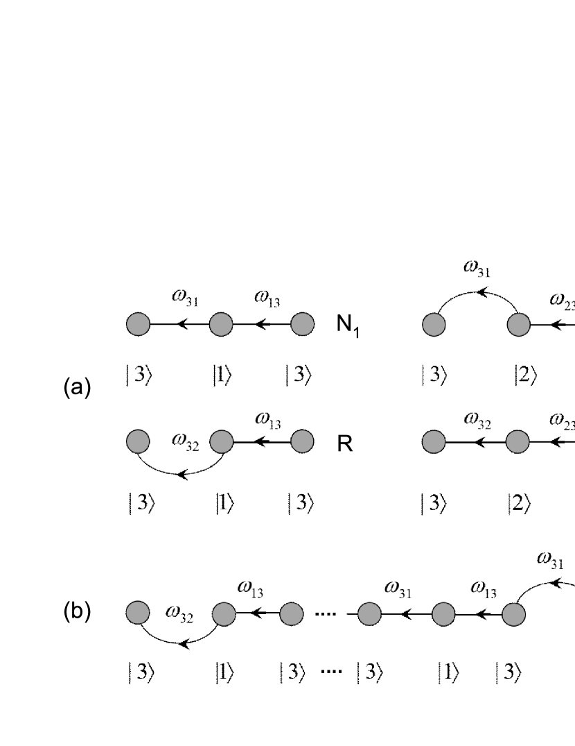
Figure 2: (a) Diagrammatic representations of four types of cycles. They are uniquely designated by the specific collapsed quantum states and exchanged quanta. Note that we refer to the N₁-cycle and N₂-cycle as the same N-cycle for the remainder of this work. (b) An example illustrates a QJT as a random combination of the three types of cycles.

IV Statistics of cycles

A careful inspection of Fig. (1)(b) indicates that a QJT in which the atom starts from state $|1\rangle$ and evolves continuously until it collapses into state $|3\rangle$ with the absorption of quantum $\omega_{32}$ uniquely specifies the R-cycle. A similar observation applies to the H-cycle. Therefore, the statistics of the two cycles correspond to the counting statistics of these two specific QJTs. Taking the R-cycle as an example, its statistical properties are obtained by solving the scaled cumulant generating function (SCGF) $\varphi(\lambda)$, which is the largest real root of the algebraic equation [57, 61],

$$\hat{p}_{1|3}(\nu)\left(\hat{p}_{3|1}^{(1)}(\nu)+\hat{p}_{3|1}^{(2)}(\nu)e^{\lambda}\right)+\hat{p}_{2|3}(\nu)\left(\hat{p}_{2|3}^{(1)}(\nu)+\hat{p}_{2|3}^{(2)}(\nu)\right)=1,$$ (17)

where $\lambda$ is the CGF parameter. An explanation of this equation is provided in Appendix B. Substituting the concrete WTDs (A), we see that Eq. (17) reduces to a quartic equation. Its radical solutions are complicated. Because the SCGF provides much statistical information, here, we focus on the mean $\overline{{\cal C}}_{R}$ and fluctuation strength $F_{R}$ of the R-cycle rate. Aided by Eqs. (37) and (38), we solve

$$\overline{{\cal C}}_{R} = \frac{2\Omega^{2}}{D}r_{1}^{-}r_{2}^{+},$$ (18)

$$F_{R} = \lim_{t\rightarrow\infty}t\text{Var}[{\cal C}_{R}]=\overline{{\cal C}}_{R}-\frac{4E\Omega^{4}}{D^{3}}(r_{1}^{-}r_{2}^{+})^{2},$$ (19)

where $D$ and $E$ are

$$D = 2\Omega^{2}\left[r_{1}^{+}+r_{2}^{+}+2(r_{1}^{-}+r_{2}^{-})\right]+\frac{1}{2}(r_{1}^{+}+r_{2}^{+})\left(r_{1}^{+}r_{2}^{+}+r_{1}^{+}r_{2}^{-}+r_{1}^{-}r_{2}^{+}\right),$$ (20)

$$E = 8\Omega^{2}+(r_{1}^{+})^{2}+(r_{2}^{+})^{2}+4r_{1}^{+}r_{2}^{+}+r_{1}^{+}r_{1}^{-}+r_{2}^{+}r_{2}^{-}+3(r_{1}^{+}r_{2}^{-}+r_{1}^{-}r_{2}^{+}),$$ (21)

respectively. Analogously, we solve the mean and fluctuation strength of the H-cycle rate. However, owing to the symmetry in the WTDs, these two formulas can be derived by exchanging indices $1$ and $2$ in Eqs. (18) and (19). Note that $D$ and $E$ are invariant under this operation. Figure (3)(a) shows the statistical quantities of the two rates under a set of parameters, in which the distribution $n_{1}$ is varied and $n_{2}$ is fixed at a certain value. The features of the mean rate curves are similar to those of the fluctuation strength curves in each type of cycle. In addition, the intersection points of these curves occur at $n_{1}=n_{2}$, which are apparent according to Eqs. (18) and (19).

Let us examine Fig. (3)(a). First, the intersection point of the mean rate curves denotes a transition of the operation of the SSDB machine from a refrigerator to a heat engine. The reason is explained in Eq. (16): By taking the time average of the equation, we obtain

$$\overline{\cal M}=\frac{2\Omega^{2}}{D}(r_{1}^{+}r_{2}^{-}-r_{1}^{-}r_{2}^{+})\propto(n_{1}-n_{2}),$$ (22)

and the power output $\cal P$ is proportional to $\cal M$. Here, a “bar” placed over a symbol denotes a mean in time. The transition condition $n_{1}=n_{2}$ is consistent with that derived at the ensemble level [13]. Second, when the SSDB operates as a heat engine, a further increase in the population $n_{1}$ above a threshold value decreases the output power. We mark the threshold value with an arrow in the figure. A similar observation is presented in the fully quantum SSDB model [25]. Because the energy levels of the atom are considered given, changes in $n_{1}$ are equivalent to changes in the temperature $T_{1}$ of the hot bath. We expect that, with the temperature of the cold bath held constant, the higher the temperature of the hot bath is, the greater the power output.

IV.1 Probabilities of cycles

To understand the counterintuitive second result, we revisit the R-cycle and H-cycle rates. Taking the R-cycle as an example, in addition to the definition given in Eq. (16), its rate has an alternative expression:

$${\cal C}_{R} = \frac{\#[\text{cycles}]}{t}{\times}\frac{\#[\text{R-cycles}]}{\#[{\rm cycles}]}.$$ (23)

The first term on the right-hand side of Eq. (23) represents the number of cycles per unit time. We call this property the cycle rate and denote it as $\cal C$. The second term in Eq. (23) is the ratio of the number of R-cycles to the total number of cycles in a QJT. Hence, it approximates the probability $P_{R}$ of a cycle being the R-type. In the large time limit, the approximation becomes exact. Therefore, Eq. (23) reduces to $\overline{\cal C}_{R}=\overline{\cal C}P_{R}$. In terms of the Laplace transforms of the WTDs, the probability is equal to

$$P_{R}=\hat{p}^{(2)}_{31}(0)\hat{p}_{13}(0).$$ (24)

For the H-cycle rate, we have an analogous equation, $\overline{\cal C}_{H}=\overline{\cal C}P_{H}$, where the probability of a cycle being H-type is

$$P_{H}=\hat{p}^{(1)}_{32}(0)\hat{p}_{23}(0).$$ (25)

Finally, there is an N-cycle rate, ${\cal C}_{N}$. Its mean is $\overline{\cal C}_{N}=\overline{\cal C}P_{N}$, where $P_{N}=1-P_{H}-P_{R}$ is the probability of a cycle being neutral. Note that if the N-cycle rate were absent, we would obtain an incorrect identity:

$$\overline{\cal C}_{R}+\overline{\cal C}_{N}=\overline{\cal C}.$$ (26)

We derive the mean cycle rate via Eq. (18) and the Laplace transforms of the WTDs (A):

$$\overline{\cal C}=\frac{1}{2D}(4\Omega^{2}+r_{1}^{+}r_{2}^{+})(r_{1}^{+}+r_{2}^{+})(r_{1}^{-}+r_{2}^{-}).$$ (27)

Note that this value is also equal to half of the mean activity [62], which is explained in Appendix B. The data show that Eq. (27) is a monotonically increasing function of $n_{1}$. Consequently, in Fig. (3)(a), the observed nonmonotonic feature of the $\overline{\cal C}_{H}$ curve is attributed to the probability $P_{H}$. To illustrate this aspect, we depict $P_{R}$, $P_{H}$, and $P_{N}$ under the same set of parameters in Fig. (3)(b). We note that the probability $P_{N}$ strongly suppresses the other two probabilities when the population $n_{1}$ is greater than $n_{2}$. Thus, we obtain the following conclusion. With larger $n_{1}$ values or at higher temperatures $T_{1}$, the SSDB machine becomes more active or operates at a higher cyclic frequency. However, the rapid increase in the number of N cycles leads to a corresponding decrease in the number of the other two cycle types.

We close this section by mentioning that the statistics of $\cal M$ can be directly derived through its original definition, the first equation in Eq. (15), without resorting to Eq. (16). Kalaee et al. derived its mean $\overline{\cal M}$ and fluctuation strength via the FCS [27]. Appendix B provides an alternative derivation via the SMP method. Although $\overline{\cal M}$ must be the same as that in Eq. (22), the equation now has a cyclic explanation. Another informative formula is the fluctuation strength

$$F_{\cal M} = \overline{\cal C}_{H}+\overline{\cal C}_{R}-\frac{4E\Omega^{4}}{D^{3}}(r_{1}^{+}r_{2}^{-}-r_{1}^{-}r_{2}^{+})^{2}$$ (28)

$$= F_{H}+F_{R}+\frac{8E\Omega^{4}}{D^{3}}r_{1}^{+}r_{1}^{-}r_{2}^{+}r_{2}^{-}.$$ (29)

Equation (28) is derived by the original definition. We emphasize that this equation cannot be obtained from the definition in Eq. (16). Equation (29) is a simple consequence of substitutions of $F_{R}$ and $F_{H}$. Over a large but finite duration, Eq. (29) implies that the covariance of ${\cal C}_{H}$ and ${\cal C}_{R}$ is nonzero and negative. Hence, the H-cycle and R-cycle rates are negatively correlated. The reason is understandable. A cycle is either a heat engine, refrigerator, or neutral. If the likelihood of a cycle being heat engine increased, the other likelihood including being refrigerator would decrease.

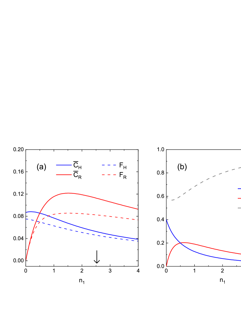
Figure 3: (a) Mean rates and fluctuation strengths of the R-cycle and H-cycle rates. The arrow denotes the threshold value at which the power output of the SSDB machine starts to decrease if $n_{1}$ further increases. Note that the mean H-cycle rate has already exceeded its maximum and starts to decrease before reaching the threshold value. (b) Probabilities that cycles are H, R, and N cycles. In both panels, the $x$-axis is the population $n_{1}$. The fixed parameters are $\omega_{31}=3$, $\omega_{32}=1$, $r_{1}=r_{2}=1$, $n_{2}=0.5$, and $\Omega=0.5$. Because we set $T_{1}>T_{2}$ in this paper, the minimum value of $n_{1}$ is given by $1/((1+1/n_{2})^{w31/w32}-1)=0.0384$.

V Efficiency and coefficient of performance

We prove that the heat engine’s efficiency and the refrigerator’s coefficient of performance (COP) of the SSDB machine are constant rather than fluctuating. In the large time limit, given a QJT $\bf X$, the efficiency and COP in the trajectory are

$$\eta_{e} = \frac{A[\bf X]}{Q_{1}[\bf X]}=\frac{\omega_{21}}{\omega_{31}},$$ (30)

$$c_{p} = -\frac{Q_{2}[\bf X]}{A[{\bf X}]}=\frac{\omega_{32}}{\omega_{21}},$$ (31)

respectively. Here, we substituted Eqs. (12)-(14) into Eqs. (30) and (31), respectively. Intriguingly, Eq. (30) is precisely the SSDB’s maser efficiency formula [1].

VI Conclusions

In this paper, we explore cycles in the QJTs of the SSDB machine. Although the quantum thermal machine is often thought of as operating cyclically, the explicit cyclic structure and precise thermodynamic meaning of the cycles are ambiguous. In the QJTs, we identify cyclic structures that can be classified into three types: H-, R-, and N-cycles. Accordingly, in each cycle, the machine operates as a heat engine, refrigerator, or neutral. In a QJT with a long duration, the SSDB machine operates by randomly switching between these three cycle types. We emphasize that the H-cycle and R-cycle are not opposite processes, since each cycle has two states, but one of the two states is not the same. Therefore, statements used in classical thermal machines, such as completing one cycle in the three states in sequence and concepts of clockwise (forward) and counterclockwise (backward) cycles, are inappropriate in the quantum case. In addition to the notion and picture, we also study the statistical properties of these three cycles via the SMP method. We find that the power output of the SSDB machine actually decreases if the hot bath temperature exceeds a certain threshold value. From a cyclic perspective, this decrease is attributed to the probability of the machine being neutral surpassing the probabilities of the other two cycle types. Note that the mean cycle rate actually increases under this situation. We finally demonstrate that the heat engine’s efficiency and the refrigerator’s COP are constant in a single QJT. This constancy results from the unique structure of the SSDB machine.

Acknowledgments We are grateful for the discussions on quantum heat engines with Shihao Xia and Prof. Shanhe Su during this work. We also express our gratitude to Prof. Jianhui Wang for his inspiring discussion on stochastic efficiency. This work was supported by the National Natural Science Foundation of China under Grant Nos. 12075016 and 11575016.

Appendix A Laplace transforms of the waiting time distributions

According to Eqs. (4) and  (5) and the non-Hermitian Hamiltonian (6), we calculate the Laplace transforms of the WTDs with respect to age:

$$\hat{p}_{3|1}^{(1)}(\nu) = r_{1}^{+}\frac{v^{2}-v(h_{+}+h_{-}-r_{2}^{+})+2h_{+}h_{-}+(r_{2}^{+})^{2}/2}{(v-2h_{+})(v-2h_{-})[v-(h_{+}+h_{-})]},$$

$$\hat{p}_{3|1}^{(2)}(\nu) = r_{2}^{+}\frac{2\Omega^{2}}{(v-2h_{+})(v-2h_{-})[v-(h_{+}+h_{-})]},$$ (32)

$$\hat{p}_{1|3}(\nu) = r_{1}^{-}\frac{1}{v+(r_{1}^{-}+r_{2}^{-})},$$

and other expressions that include $\hat{p}_{3|2}^{(1)}$, $\hat{p}_{1|3}^{(2)}$, and $\hat{p}_{2|3}$ are obtained by exchanging indices $1$ and $2$ in Eq. (A), e.g.,

$$\hat{p}_{3|2}^{(2)}(\nu) = r_{2}^{+}\frac{v^{2}-v(h_{+}+h_{-}-r_{1}^{+})+2h_{+}h_{-}+(r_{1}^{+})^{2}/2}{(v-2h_{+})(v-2h_{-})[v-(h_{+}+h_{-})]}.$$

Here, $h_{+}$ and $h_{-}$ are two roots of a quadratic equation: $h_{+}+h_{-}=-(r_{1}^{+}+r_{2}^{+})/2$ and $h_{+}h_{-}=\Omega^{2}+r_{1}^{+}r_{2}^{+}/4$. Symmetry arises from the resonant condition in which the detuning parameter is zero. When the discriminant $(r_{1}^{+}-r_{2}^{+})^{2}-16\Omega^{2}$ is positive or negative, the two roots can be both real numbers or complex conjugates to each other. Correspondingly, in the time domain, the WTDs $p^{(j)}_{3|i}$ and $i,j=1,2$ are multiexponential decay and oscillatory decay, respectively. Equation (A) has a useful property: At $\nu=0$, these transforms are just the transition probabilities of the Markov chain in the SMP [57].

Appendix B Semi-Markov process method

In the main text, we noted that the statistics of the R-cycle are equivalent to the counting statistics of the specific QJT. Let the random variable ${\cal C}_{R}$ have the distribution $p_{R}(c)$. Its statistics can be obtained via finding the CGF, the logarithm of the Laplace transform of the distribution. In the large time limit, the SCGF

$$\varphi(\lambda)=\lim_{t\rightarrow\infty}\frac{1}{t}\ln\langle e^{\lambda tc}\rangle$$ (33)

is more useful [60], where $\langle\cdots\rangle$ denotes an average over the distribution. The SMP method can solve SCGFs in open quantum systems [57, 61]. The core of the method is that the SCGF of ${\cal C}_{R}$ is equal to the largest real root of the equation of poles:

$$\det[{\mathbb{I}}-{\mathbb{W}}(\nu,\lambda)]=0.$$ (34)

where $\mathbb{I}$ is a $3\times 3$ unit matrix and

$$\mathbb{W}(\nu,\lambda)=\begin{bmatrix}0&0&\hat{p}_{1|3}(\nu)\\ 0&0&\hat{p}_{2|3}(\nu)\\ \hat{p}^{(1)}_{3|1}(\nu)+\hat{p}^{(2)}_{3|1}(\nu)e^{\lambda}&\hat{p}^{(1)}_{3|2}(\nu)+\hat{p}^{(2)}_{3|2}(\nu)&0.\\ \end{bmatrix}$$ (35)

Here, the structure of the matrix $\mathbb{W}$ already considers the characteristics of the WTDs in the SSDB machine. The SMP method has been described previously [57, 61]. Here, we summarize a rule for writing the matrix $\mathbb{W}$: When a specific QJT is counted, in which the atom starts in quantum state $|i\rangle$, $i=1,2$, continuously evolves, and first collapses into state $|3\rangle$ by a certain jumping operator $\sigma_{3j}$, $j=1,2$, the Laplace transform of the WTD $\hat{p}^{(j)}_{3|i}$ in the matrix is multiplied with $\exp(\lambda)$; when another specific QJT is counted, in which the atom starts $|3\rangle$, continuously evolves, and first collapses into state $|i\rangle$, $i=1,2$, the Laplace transform of the WTD $\hat{p}_{i|3}$ is multiplied by $\exp(\lambda)$.

In general, the equation of poles (34) reduces to a higher-order algebraic equation. Hence, finding its roots or the SCGFs analytically is usually difficult. However, the first two moments can be derived analytically. First, we transform Eq. (34) into a polynomial in $\nu$ by removing all denominators and let the left-hand side be $P(\nu,z)$ with $z=\exp(\lambda)$. Following the definition of the CGF, we have

$$\left.P(v,z)\right|_{v=0,z=1}=0.$$ (36)

Second, by taking derivatives up to second order, we derive

$$\frac{d\nu}{d\lambda}(0) = -\left.\frac{\partial_{z}P}{\partial_{\nu}P}\right|_{\nu=0,z=1},$$ (37)

$$\frac{d^{2}\nu}{d\lambda^{2}}(0) = -\left.\frac{1}{\partial_{\nu}P}\left[\left(\frac{d\nu}{d\lambda}\right)^{2}\partial_{\nu}^{2}P+2\left(\frac{d\nu}{d\lambda}\right)\partial_{\nu z}^{2}P+\partial_{z}^{2}P+\partial_{z}P\right]\right|_{\nu=0,z=1}.$$ (38)

Finally, considering $\nu$ as the SCGF $\varphi(\lambda)$, Eqs. (37) and (38) are the mean and fluctuation strength of the R-cycle rate, respectively. The procedure for calculating the statistics of the R-cycle rate also applies to the H-cycle rate. The only modification is to shift the position of $e^{\lambda}$ from after $\hat{p}^{(2)}_{3|1}$ to after $\hat{p}^{(1)}_{3|2}$.

We still need to calculate the counting statistics for ${\cal C}$, the cycle rate, and $\cal M$, the net number of quanta $\omega_{31}$ absorbed by the atom from the $T_{1}$-heat bath per unit time. Similarly, modifications are made to matrix $\mathbb{W}$. For $\cal C$, Fig. (2)(b) indicates that a cycle is completed when specific QJTs that start from state $|3\rangle$ and end in state $|1\rangle$ or $|2\rangle$ for the first time are counted. Accordingly, the matrix is modified as follows:

$$\mathbb{W}(\nu,\lambda)=\begin{bmatrix}0&0&\hat{p}_{1|3}(\nu)e^{\lambda}\\ 0&0&\hat{p}_{2|3}(\nu)e^{\lambda}\\ \hat{p}^{(1)}_{3|1}(\nu)+\hat{p}^{(2)}_{3|1}(\nu)&\hat{p}^{(1)}_{3|2}(\nu)+\hat{p}^{(2)}_{3|2}(\nu)&0\\ \end{bmatrix}.$$ (39)

A comment is in order. Ref. [62] proposed the notion of activity. In the context of the QJTs, activity refers to the number of wave functions that collapse per unit time. Its statistics are derived from another $\mathbb{W}$, in which all Laplace transforms of the WTDs are multiplied by $\exp(\lambda)$. The equation of poles for the newly mentioned matrix is identical to that of Eq. (39) if the $\lambda$ in the latter is replaced by $2\lambda$. Thus, we mathematically demonstrate that the mean activity is twice the mean cycle rate. Since two collapses occur in any cycle, this conclusion is easily understood. For the random variable ${\cal M}$, the matrix is

$$\mathbb{W}(\nu,\lambda)=\begin{bmatrix}0&0&\hat{p}_{1|3}(\nu)e^{-\lambda}\\ 0&0&\hat{p}_{2|3}(\nu)\\ \hat{p}^{(1)}_{3|1}(\nu)e^{\lambda}+\hat{p}^{(2)}_{3|1}(v)&\hat{p}^{(1)}_{3|2}(\nu)e^{\lambda}+\hat{p}^{(2)}_{3|2}(\nu)&0\\ \end{bmatrix}.$$ (40)

Note that $\exp(-\lambda)$ after $\hat{p}_{1|3}(\nu)$ in Eq. (40) indicates that the $T_{1}$-heat bath absorbs a quantum $\omega_{31}$ from the atom rather than the reverse process.

We briefly explain why we chose the SMP method instead of the more popular FCS [41, 32, 63, 33, 64, 65]. To solve the SCGFs, the FCS similarly involves finding the largest real eigenvalue of the tilted generator of the QME. We have demonstrated that these two methods are equivalent when calculating the statistics of certain special random variables, such as those previously mentioned $\cal C$ and $\cal M$. However, the FCS is unsuited for the H-cycle and R-cycle rates that are of interest in this paper. For more explanations, we refer to our previous paper [57].

References

- [1] H. E. D. Scovil and E. O. Schulz-DuBois. Three-level masers as heat engines. Phys. Rev. Lett., 2:262–263, Mar 1959.
- [2] Robert Alicki and Ronnie Kosloff. Introduction to quantum thermodynamics: History and prospects. In Fundamental Theories of Physics, pages 1–33. Springer International Publishing, 2018.
- [3] J. E. Geusic, E. O. Schulz-DuBios, and H. E. D. Scovil. Quantum equivalent of the carnot cycle. Phys. Rev., 156:343–351, Apr 1967.
- [4] Robert Alicki. On the detailed balance condition for non-hamiltonian systems. Rep. Math. Phy., 10(2):249–258, 1976.
- [5] H. Spohn and J. L Lebowitz. Irreversible thermodynamics for quantum systems weakly coupled to thermal reservoirs. In Adv. Chem. Phys, volume 39, pages 109–141, 1978.
- [6] Herbert Spohn. Entropy production for quantum dynamical semigroups. J. Math. Phys., 19(5):1227, 1978.
- [7] R Kosloff. A quantum mechanical open system as a model of a heat engine. J. Chem. Phys., 80:1625, 1984.
- [8] Eitan Geva and Ronnie Kosloff. Three-level quantum amplifier as a heat engine: A study in finite-time thermodynamics. Phys. Rev. E, 49(5):3903, 1994.
- [9] Tova Feldmann and Ronnie Kosloff. Performance of discrete heat engines and heat pumps in finite time. Phys. Rev. E, 61:4774–4790, May 2000.
- [10] J; Hua B. He, J; Chen. Quantum refrigeration cycles using spin-1/2 systems as the working substance. Phys. Rev. E, 65:036145, 2002.
- [11] H. Walther M. O. Scully M. S. Zubairy, G. S. Agarwal. Extracting work from a single heat bath via vanishing quantum coherence. Science, 299(5608):862–864, January 2003.
- [12] C.P. Sun H.T. Quan, Y.X. Liu and F. Nori. Quantum thermodynamic cycles and quantum heat engines. Phy. Rev. E, 76:031105, 2007.
- [13] E. Boukobza and D. J. Tannor. Three-level systems as amplifiers and attenuators: A thermodynamic analysis. Phys. Rev. Lett., 98:240601, Jun 2007.
- [14] Dvira Segal. Stochastic pumping of heat: Approaching the carnot efficiency. Phys. Rev. Lett., 101:260601, Dec 2008.
- [15] Armen E. Allahverdyan, Karen V. Hovhannisyan, Alexey V. Melkikh, and Sasun G. Gevorkian. Carnot cycle at finite power: Attainability of maximal efficiency. Phys. Rev. Lett., 111:050601, Aug 2013.
- [16] Shan-He Su, Chang-Pu Sun, Sheng-Wen Li, and Jin-Can Chen. Photoelectric converters with quantum coherence. Phys. Rev. E, 93:052103, May 2016.
- [17] J. Rossnagel, S. T. Dawkins, K. N. Tolazzi, O. Abah, E. Lutz, F. Schmidt-Kaler, and K. Singer. A single-atom heat engine. Science, 352(6283):325–329, apr 2016.
- [18] Bijay Kumar Agarwalla, Jian-Hua Jiang, and Dvira Segal. Quantum efficiency bound for continuous heat engines coupled to noncanonical reservoirs. Phys. Rev. B, 96(10):104304, September 2017.
- [19] Chen Wang, Jie Ren, and Jianshu Cao. Unifying quantum heat transfer in a nonequilibrium spin-boson model with full counting statistics. Phys. Rev. A, 95:023610, Feb 2017.
- [20] John P. S. Peterson, Tiago B. Batalhão, Marcela Herrera, Alexandre M. Souza, Roberto S. Sarthour, Ivan S. Oliveira, and Roberto M. Serra. Experimental characterization of a spin quantum heat engine. Phys. Rev. Lett., 123:240601, Dec 2019.
- [21] Quentin Bouton, Jens Nettersheim, Sabrina Burgardt, Daniel Adam, Eric Lutz, and Artur Widera. A quantum heat engine driven by atomic collisions. Nat. Commun., 12(1), April 2021.
- [22] Yang Xiao, Dehua Liu, Jizhou He, Lin Zhuang, Wu-Ming Liu, L.-L Yan, and Jianhui Wang. Thermodynamics and fluctuations in finite-time quantum heat engines under reservoir squeezing. Phys. Rev. Res., 5:043185, Nov 2023.
- [23] Jennifer Koch, Keerthy Menon, Eloisa Cuestas, Sian Barbosa, Eric Lutz, Thomas Fogarty, Thomas Busch, and Artur Widera. A quantum engine in the bec-bcs crossover. Nature, 621(7980):723–727, September 2023.
- [24] Dvira Segal. Current fluctuations in quantum absorption refrigerators. Phys. Rev. E, 97:052145, May 2018.
- [25] Sheng-Wen Li, Moochan B. Kim, Girish S. Agarwal, and Marlan O. Scully. Quantum statistics of a single-atom scovil–schulz-dubois heat engine. Phys. Rev. A, 96:063806, Dec 2017.
- [26] Varinder Singh. Optimal operation of a three-level quantum heat engine and universal nature of efficiency. Phys. Rev. Res., 2:043187, Nov 2020.
- [27] Alex Arash Sand Kalaee, Andreas Wacker, and Patrick P. Potts. Violating the thermodynamic uncertainty relation in the three-level maser. Phys. Rev. E, 104:L012103, Jul 2021.
- [28] Paul Menczel, Eetu Loisa, Kay Brandner, and Christian Flindt. Thermodynamic uncertainty relations for coherently driven open quantum systems. J. Phys. A: Math. Theor., 54(31):314002, jul 2021.
- [29] Ronnie Kosloff. Quantum thermodynamics: A dynamical viewpoint. Entropy, 15(6):2100–2128, 2013.
- [30] Ronnie Kosloff and Amikam Levy. Quantum heat engines and refrigerators: Continuous devices. Annu. Rev. Phys. Chem., 65(1):365–393, 2014.
- [31] Denis J. Evans, E. G. D. Cohen, and G. P. Morriss. Probability of second law violations in shearing steady states. Phys. Rev. Lett., 71:2401–2404, Oct 1993.
- [32] Joel L. Lebowitz and Herbert Spohn. J. Stat. Phys., 95(1/2):333–365, 1999.
- [33] Massimiliano Esposito, Upendra Harbola, and Shaul Mukamel. Nonequilibrium fluctuations, fluctuation theorems, and counting statistics in quantum systems. Rev. Mod. Phys., 81(4):1665, 2009.
- [34] Christopher Jarzynski. Annu. Rev. Condens. Matter Phys., 2:329–351, 2011.
- [35] Udo Seifert. Stochastic thermodynamics: An introduction. In Nonequilibrium Statistical Physics Today: Granada Seminar on Computational & Statistical Physics, pages 56–76, 2011.
- [36] Michele Campisi, Peter Hänggi, and Peter Talkner. Colloquium: Quantum fluctuation relations: Foundations and applications. Rev. Mod. Phys., 83(3):771, 2011.
- [37] Andre C. Barato and Udo Seifert. Thermodynamic uncertainty relation for biomolecular processes. Phys. Rev. Lett., 114:158101, Apr 2015.
- [38] Todd R. Gingrich, Jordan M. Horowitz, Nikolay Perunov, and Jeremy L. England. Dissipation bounds all steady-state current fluctuations. Phys. Rev. Lett., 116:120601, Mar 2016.
- [39] Vittorio Gorini, Andrzej Kossakowski, and Ennackal Chandy Georgec Sudarshan. Completely positive dynamical semigroups of n-level systems. J. Math. Phys., 17(5):821–825, 1976.
- [40] Goran Lindblad. On the generators of quantum dynamical semigroups. Comm. Math. Phys., 48(2):119–130, 1976.
- [41] B. R. Mollow. Pure-state analysis of resonant light scattering: Radiative damping, saturation, and multiphoton effects. Phys. Rev. A, 12:1919–1943, Nov 1975.
- [42] M.D. Srinivas and E.B. Davies. Photon counting probabilities in quantum optics. Opt. Acta., 28(7):981–996, 1981.
- [43] M. O. Scully and M. S. Zubairy. Quantum Optics. Cambridge University Press, Cambridge, 1997.
- [44] Heinz-Peter Breuer and Francesco Petruccione. The theory of open quantum systems. Oxford university press, Oxford, 2002.
- [45] Howard M Wiseman and Gerard J Milburn. Quantum measurement and control. Cambridge University Press, Cambridge, 2010.
- [46] Heinz-Peter Breuer. Genuine quantum trajectories for non-markovian processes. Phys. Rev. A, 70:012106, Jul 2004.
- [47] Wojciech De Roeck and Christian Maes. Quantum version of free-energy–irreversible-work relations. Phys. Rev. E, 69(2):026115, 2004.
- [48] Jordan M Horowitz. Quantum-trajectory approach to the stochastic thermodynamics of a forced harmonic oscillator. Phys. Rev. E, 85(3):031110, 2012.
- [49] F W J Hekking and J P Pekola. Quantum jump approach for work and dissipation in a two-level system. Phys. Rev. Lett., 111(9):093602, 2013.
- [50] Fei Liu. Equivalence of two bochkov-kuzovlev equalities in quantum two-level systems. Phys. Rev. E, 89:042122, Apr 2014.
- [51] Fei Liu and Jingyi Xi. Characteristic functions based on a quantum jump trajectory. Phys. Rev. E, 94:062133, Dec 2016.
- [52] Fei Liu and Shanhe Su. Stochastic floquet quantum heat engines and stochastic efficiencies. Phys. Rev. E, 101:062144, Jun 2020.
- [53] Paul Menczel, Christian Flindt, and Kay Brandner. Quantum jump approach to microscopic heat engines. Phys. Rev. Res., 2:033449, Sep 2020.
- [54] Howard Carmichael. An open systems approach to Quantum Optics, volume 18. Springer, Berlin, 1993.
- [55] Klaus Mølmer, Yvan Castin, and Jean Dalibard. Monte carlo wave-function method in quantum optics. J. Opt. Soc. Am. B, 10(3):524–538, Mar 1993.
- [56] M.B. Plenio and P.L. Knight. The quantum-jump approach to dissipative dynamics in quantum optics. Rev. Mod. Phys., 70(1):101, 1998.
- [57] Fei Liu. Semi-markov processes in open quantum systems: Connections and applications in counting statistics. Phys. Rev. E, 106:054152, Nov 2022.
- [58] In this paper, we neglect noncycle parts of the QJTs, if any, at the beginning and ending of the trajectories, which is reasonable considering the large time limit.
- [59] Mark T. Mitchison. Quantum thermal absorption machines: refrigerators, engines and clocks. Contemp. Phys., 60(2):164–187, 2019.
- [60] Hugo Touchette. The large deviation approach to statistical mechanics. Phys. Rep., 478(1-3):1–69, 2008.
- [61] F. Liu. Semi-markov processes in open quantum systems. iii. large deviations of first passage time statistics. Arxiv, 2024.
- [62] Juan P. Garrahan. Simple bounds on fluctuations and uncertainty relations for first-passage times of counting observables. Phys. Rev. E, 95:032134, Mar 2017.
- [63] D. A. Bagrets and Yu. V. Nazarov. Full counting statistics of charge transfer in coulomb blockade systems. Phys. Rev. B, 67:085316, Feb 2003.
- [64] Juan P. Garrahan and Igor Lesanovsky. Thermodynamics of quantum jump trajectories. Phys. Rev. Lett., 104(16):160601, Apr 2010.
- [65] Gabriel T. Landi, Michael J. Kewming, Mark T. Mitchison, and Patrick P. Potts. Current fluctuations in open quantum systems: Bridging the gap between quantum continuous measurements and full counting statistics. PRX Quantum, 5:020201, Apr 2024.