An Explicit Wavefunction of the Interacting Non-Hermitian Spin-1/2 1D System

Abstract

We present an explicit Bethe-ansatz wavefunction to a 1D spin-$\frac{1}{2}$ interacting fermion system, manifesting a many-body resonance resulting from the interplay between interaction and non-Hermitian spin-orbit coupling. In the dilute limit, the wavefunction is greatly simplified and then factorized into Slater determinants and a Jastrow factor. An effective thermodynamic distribution is constructed with an effective Hamiltonian including a repulsion resulting from Pauli’s exclusion principle and a distinctive zigzag potential arising from the resonance. The competition between these effects leads to a transition from a uniformly distributed configuration to a phase separation. The connection to the recent cold atom experimental efforts of realizing on-site atom-loss is discussed.

Introduction.— The non-Hermitian skin effect (NHSE) has attracted significant attentions in recent years [1, 2, 3, 4, 5]. The associated anomalous properties, such as the complex-valued spectrum and the localization on boundaries, can be described by the theory of the generalized Brillouin zone, in which momenta are complex-valued [2, 6, 7, 8, 9, 10, 11]. These distinctive features are highly sensitive to boundary conditions. For example, the eigenstates in non-Hermitian systems are usually extended under the periodical boundary condition (PBC) while localized under the open boundary condition (OBC), which contrasts to the case in Hermitian physics. Experimentally, the NHSE has been observed in various systems, including metamaterials [12, 13], photonic systems [14], electrical circuits [15, 16], acoustic crystals [17], and cold atomic systems [18].

Despite the significant progress in the NHSE, current studies predominantly focus on the single-body physics. How the NHSE behaves under strong interactions remains an open question, and non-perturbative analytical studies are desired. The Bethe-ansatz (BA) method [19, 20] is a systematic tool for studying one dimensional (1D) integrable systems, including the Lieb-Liniger model of the interacting Bose gas [21, 22], the Gaudin-Yang model of the interacting Fermi gas [23, 24], and the Lieb-Wu solution to the Hubbard model [25]. When applied to non-Hermitian systems, it has been found that NHSE is suppressed by repulsive interactions [26, 27, 28, 29, 30]. However, the complexity of BA wavefunctions makes it difficult to calculate observables. It would be desired to construct an explicit many-body wavefunction to facilitate a deeper understanding of the NHSE in interacting systems, akin to the Ogata-Shiba-type and the Laughlin-type wavefunctions [31, 32].

In this work, we present a concise expression for the many-body wavefunction in a 1D spin-1/2 fermion system with the non-Hermitian spin-orbit coupling (SOC). As a result of the strong repulsive $\delta$-interaction, each particle behaves as a soft boundary to particles with opposite spins, which induces an effective attraction between them. Resonance states are formed here instead of bound states, i.e., the Bethe string states [33, 34, 35]. The explicit many-body wavefunction is constructed in the dilute limit, which is a rare example in many-body physics. It consists of the product of Slater determinants and the Jastrow factor [36] reflecting the resonance between particles with opposite spins. Remarkably, as varying the interacting strength, a phase transition takes place that an effective “spin-diople” per resonance pair scales from a finite value to a linear divergence with the system size.

Model.—We start with the following 1D non-Hermitian many-body Hamiltonian with system length $L$ ($\hbar=1$)

$$\hat{H}=\sum_{l=1}^{N}\frac{\left(-i\nabla_{l}+im\alpha\sigma_{l}^{z}\right)^{2}}{2m}+\sum_{\langle ll^{\prime}\rangle}2g\delta\left(x_{l}-x_{l^{\prime}}\right),$$ (1)

where $\alpha>0$ represents the strength of the non-Hermitian SOC; $g>0$ represents the strength of repulsive interaction; the PBC is assumed. Since the $z$-component of total spin is conserved, the eigenvalues and many-body eigenstates can be labelled by the particle numbers of two components, i.e., $N_{\uparrow}$ and $N_{\downarrow}$. In the following, the real and imaginary parts of the complex momentum are defined as

$$k_{l,\sigma_{l}}=(\chi_{l,\sigma_{l}}+i\mathcal{\eta}_{l,\sigma_{l}})/L,$$ (2)

where $l$ is the particle number index and $\sigma_{l}$ is the spin component along the $z$-direction.

We warm up by considering the single-body problem. If the particle carries spin $\sigma$ ($\sigma=\uparrow,\downarrow$), the eigenstates are denoted as $e^{ik_{\sigma}x}|\sigma\rangle$, and the eigen-energies are $(k_{\uparrow,\downarrow}\pm im\alpha)^{2}/(2m)$, respectively. The momentum is quantized as $k_{\sigma}=2\pi n_{\sigma}/L$ under the PBC. Upon the OBC, the spin-up and down particles localize at the right and left boundaries, respectively. The single-particle localization length is $\lambda_{s}=(m\alpha)^{-1}$, which is independent of the system size, indicating the presence of bound states. This is the conventional NHSE discussed in the literature.

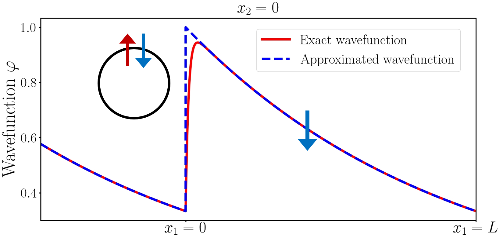
Figure 1: The 2-body wavefunction $\varphi(x_{1},x_{2})$ with particles of opposite spins by fixing the coordinate of the spin-up one $x_{2}=0$. The parameter values are $\chi_{1}=\chi_{2}=0$, $m=1$, $g=2$, $\alpha=1$ and $L=50$. The peak appears at $x_{1}\sim\ln(L\lambda_{s}^{-1})/(L\lambda_{s}^{-1})$. In the case of $L\gg\lambda_{s}$, the peak is located at $x_{1}=x_{2}$ and $\varphi$ becomes discontinuous. It implies that the spin-down particle tends to lie on the right side of the spin-up particle, forming a resonant pair on the ring.

Two-body case.— With $N_{\uparrow}=2$ and $N_{\downarrow}=0$, the corresponding eigenstate is a Slater determinant of plane wave states with $k_{i,\uparrow}=2\pi n_{i,\uparrow}/L$ and $i=1,2$. The $\delta$-interaction does not manifest here due to Pauli’s exclusion principle. The corresponding eigenenergy is $E=\sum_{i}(k_{i,\uparrow}+im\alpha)^{2}/2m$. The case with two spin-down particles can be constructed in parallel.

Non-trivial interaction effect emerges with a pair of particles of opposite spins. The eigenstate is written as $\varphi(x_{1},x_{2})|\downarrow\uparrow\rangle-\varphi(x_{2},x_{1})|\uparrow\downarrow\rangle$. Using the center of mass coordinate $X=(x_{1}+x_{2})/2$ and the relative coordinate $r=x_{1}-x_{2}$, the wavefunction is decomposed as $\varphi(x_{1},x_{2})=\Phi(X)\phi(r)$, satisfying the following equations,

$$\left\{\begin{array}[]{l}\left(-\frac{\nabla_{X}^{2}}{4m}-m\alpha^{2}\right)\Phi(X)=E_{X}\Phi(X),\vspace{1ex}\\ \left(-\frac{\nabla_{r}^{2}}{m}-2\alpha\nabla_{r}+2g\delta(r)\right)\phi(r)=E_{r}\phi(r).\end{array}\right.$$ (3)

$\Phi(X)$ is solved as $e^{iK_{X}X}$ where $K_{X}=2\pi n_{K}/L$. The non-Hermitian term $-2\alpha\nabla_{r}$ only appears in the motion of the relative coordinate, where the $\delta$-potential acts as a soft boundary. Therefore, the reminiscence of the NHSE would bring an effective attraction between two particles, explained as follows. The relative motion is solved as

$$\phi(r)=Ae^{ik_{r}r}+Be^{-ik_{r}r-2m\alpha r},$$ (4)

where $A,B$ are scattering amplitudes, $k_{r}=(\chi_{r}+i\eta_{r})/L$ is the complex momentum. Matching wavefunctions on both sides of the $\delta$-potential, it yields,

$$\frac{\beta}{g}\Big{(}(-1)^{n_{K}}\operatorname{cosh}m\alpha L-\operatorname{cosh}m\beta L\Big{)}=\operatorname{sinh}m\beta L,$$ (5)

where $\beta=\alpha+i\frac{k_{r}}{m}$. As shown in Supplemental Material (SM) A, in the case of $L\gg\lambda_{s}$, Eq. (5) is solved as

$$\left\{\begin{array}[]{l}\chi_{r}=(2n_{r}+n_{K})\pi,\ \ \ \mathcal{\eta}_{r}=\ln(1+\frac{g}{\alpha}),\vspace{1ex}\\ \frac{A}{B}=-(1+\frac{\alpha}{g}).\end{array}\right.$$ (8)

$\phi(r)$ is identical to a single-body wavefunction of spinless particle subjected to a “soft” boundary condition, which lies between the cases of OBC and PBC, since the $\delta$-potential permits partial transmission. In all cases, the solution possesses a pair of momenta, whose imaginary parts are summed to $2m\alpha$. In the OBC case, both imaginary parts equal $m\alpha$, while in the PBC case, one becomes real and the other carries the imaginary part of $2m\alpha$. In our case, a small imaginary part $\eta_{r}/L$ is at the order of $1/L$, and the other remains at the order of $2m\alpha$. Consequently, the decay of $\phi(r)$ is at the length scale of $L$, such that these states are resonance rather than bound states [37, 38]. The situation of OBC is recovered for $g\sim\frac{1}{mL}e^{L/\lambda_{s}}$ in which case the localization length $L/\eta_{r}\sim\lambda_{s}$, while that of PBC corresponds to $g=0$.

In the lab frame, $\varphi(x_{1},x_{2})$ is written as,

$$\theta(x_{1}>x_{2})\left(Ae^{i(k_{1,\downarrow}x_{1}+k_{2,\uparrow}x_{2})}+Be^{i(k_{2,\downarrow}x_{1}+k_{1,\uparrow}x_{2})}\right)$$ (9)

$$+\theta(x_{2}>x_{1})\left(A^{\prime}e^{i(k_{1,\downarrow}x_{1}+k_{2,\uparrow}x_{2})}+B^{\prime}e^{i(k_{2,\downarrow}x_{1}+k_{1,\uparrow}x_{2})}\right)$$

where $0<x_{1,2}<L$. $B$ and $B^{\prime}$-terms are the reflected waves of $A$ and $A^{\prime}$-terms respectively. After the collision, the real parts of momenta switch, but their imaginary parts change due to the SOC. For example, in the domain of $\theta(x_{1}>x_{2})$, the imaginary parts of $k_{1,\downarrow}$ and $k_{2,\uparrow}$ are at the order of $1/L$,

$$k_{1,\downarrow}=(\chi_{1}+i\mathcal{\eta}_{r})/L,\ \ \ k_{2,\uparrow}=(\chi_{2}-i\mathcal{\eta}_{r})/L,$$ (10)

where $\chi_{i}=2\pi n_{i}$ with $i=1,2$. In contrast, the imaginary parts of the reflected momenta $k_{1,\uparrow}$ and $k_{2,\downarrow}$ become finite as

$$k_{1,\uparrow}=k_{1,\downarrow}-2im\alpha,\ \ \ k_{2,\downarrow}=k_{2,\uparrow}+2im\alpha.$$ (11)

$A^{\prime}$ and $B^{\prime}$-terms are the transmitted waves of $A$ and $B$-terms respectively. The PBC yields $A^{\prime}/A=e^{ik_{1,\downarrow}L}$ and $B^{\prime}/B=e^{ik_{2,\downarrow}L}$.

We view $A$ and $A^{\prime}$-terms as the incident waves and $B$ and $B^{\prime}$-terms as the reflection ones. Due to the different behaviors of their imaginary parts, in the case of $L\gg\lambda_{s}$, the reflection channels can be dropped if the inter-particle distance exceeds $\lambda_{s}$. Then the wavefunction is simplified to the product of plane-waves and a Jastrow factor,

$$\varphi(x_{1},x_{2})=Ae^{i\left(\chi_{1}x_{1}+\chi_{2}x_{2}\right)/L}\cdot e^{-\frac{1}{2}W(x_{1}-x_{2})},$$ (12)

where $e^{-\frac{1}{2}W(x_{1}-x_{2})}$ is given by the sum of step-functions modified by the imaginary parts of the complex momentum

$$e^{-\eta_{r}(x_{1}-x_{2})/L}\left(\theta(x_{1}>x_{2})+\theta(x_{2}>x_{1})\left(1+\frac{g}{\alpha}\right)^{-1}\right).$$

More explicitly,

$$W(r)=\begin{cases}2\eta_{r}\frac{r}{L},&0<r<L\vspace{1ex}\\ 2\eta_{r}(\frac{r}{L}+1),&-L<r<0\end{cases},$$ (13)

which exhibits a jump at $r=0$.

The exact and approximated wavefunctions Eq. (9) and Eq. (12) are illustrated in Fig. 1 respectively. The spin-up particle is fixed at $x_{2}=0$. Increasing $x_{1}$ from $0$, $\varphi(x_{1},x_{2})$ rapidly reaches the peak located at $x_{1,\rm peak}\sim\ln(L\lambda_{s}^{-1})/(L\lambda_{s}^{-1})$. If $L\gg\lambda_{s}$, $x_{1,\rm peak}$ coincides with $x_{2}$. The peak is followed by a slow decay at the length scale of $L$. The behavior at $x_{1}<0$ can be obtained by applying the PBC. The spin-down particle prefers the right side of the spin-up one, which can be understood as a weaker version of the NHSE.

The energy eigenvalue is $E=(k_{1,\downarrow}-im\alpha)^{2}/2m+(k_{2,\uparrow}+im\alpha)^{2}/2m$, where $k_{1,\downarrow}$and $k_{2,\uparrow}$ are complex. The $\delta$-interaction only modifies the allowed values of the momenta, whose imaginary parts always tend to reduce the effect of non-Hermitian SOC. As we will explain later, the two-body wavefunction can be generalized to the many-body case, in which the above picture still holds.

Many-body problem: BA equations.— For eigenstates with $N_{\downarrow}$ down spins and $N_{\uparrow}=N-N_{\downarrow}$ up spins, the corresponding BA equations are [39]:

$$\prod_{i=1}^{N_{\downarrow}}\!\frac{\Lambda_{i}-\overline{k}_{l}-img}{\Lambda_{i}-\overline{k}_{l}+img}\!=\!e^{i\overline{k}_{l}L}e^{m\alpha L},$$ (14)

$$\prod_{l=1}^{N}\!\frac{\Lambda_{i}-\overline{k}_{l}-img}{\Lambda_{i}-\overline{k}_{l}+img}\!=\!-e^{2m\alpha L}\prod_{i^{\prime}=1}^{N_{\downarrow}}\!\frac{\Lambda_{i}-\Lambda_{i^{\prime}}-2img}{\Lambda_{i}-\Lambda_{i^{\prime}}+2img},$$

where $\{\overline{k}_{l}\}$ and $\{\Lambda_{i}\}$ are $N$ and $N_{\downarrow}$ variables to be determined, with $1\leq l\leq N$ and $1\leq i,i^{\prime}\leq N_{\downarrow}$. Once $\{\bar{k}_{l}\}$ are obtained, the corresponding momentum of the $l$-th particle with spin $\sigma_{l}$ is given by

$$k_{l,\sigma_{l}}=\overline{k}_{l}-im\alpha\sigma_{l}.$$ (15)

It would be challenging to solve $\{\bar{k}_{l}\}$ from the BA equations. Actually it is significantly simplified due to the non-Hermitian SOC. Among all the scattering channels, there is a specific one with momentum distribution

$$k_{i,\downarrow} = (\chi_{i}+i\mathcal{\eta}_{r}N_{\uparrow})/L,~{}~{}k_{j,\uparrow}=(\chi_{j}-i\mathcal{\eta}_{r}N_{\downarrow})/L,$$ (16)

where $1\leq i\leq N_{\downarrow}$, $N_{\downarrow}+1\leq j\leq N$, $\chi_{l}=2\pi n_{l}$ and $\mathcal{\eta}_{r}$ is defined in Eq. (8). We denote this channel as the incident wave, in which the imaginary parts of momenta are small in the dilute limit. Similar to the two-body case, reflection between spin-up and down particles will cause a pair of momenta to carry finite imaginary parts at the order of $m\alpha=\lambda_{s}^{-1}$. These reflected waves decay much faster than the incident wave, therefore can be discarded in the dilute limit defined as,

$$\frac{d}{\lambda_{s}}\gg\ln\left(1+\frac{g}{\alpha}\right),$$ (17)

where $d=L/N$ is the average inter-particle distance. Detailed calculations are found in the SM. B. Note that our approximated solution exhibits a singularity at $\alpha=0$, since the dilute limit is broken in that case.

Comparing Eq. (16) with the two-body solution Eq. (10), one finds that only imaginary parts of momenta change, which are amplified by the number of particles with opposite spins. This fact stems from the nature of resonant states. For a spin-down particle, it deems each spin-up particle as a soft boundary, such that its length free of collision is roughly $L/N_{\uparrow}$. Hence, the imaginary part of $k_{i,\downarrow}$ in Eq. (16) is amplified by a factor of $N_{\uparrow}$. The case for a spin-up particle is in parallel.

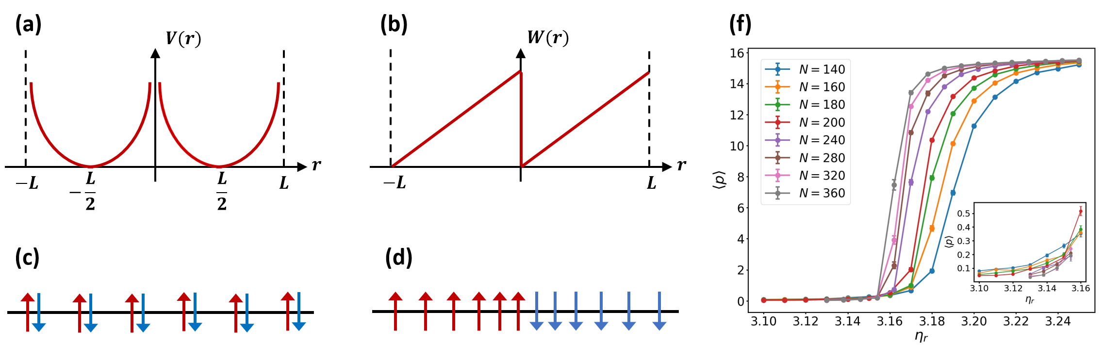
Figure 2: ($a$) and ($b$) plots $V(r)$ and $W(r)$, the effective potentials arising from transforming the BA wavefunction into a thermodynamic distribution shown in Eq. (20). Configuration ($c$) or ($d$) is favored when $V$ or $W$ is dominant, respectively. The former exhibits a finite value of dipole strength $p$, while $p$ diverges linearly with $L$ in the latter case. The Monte-Carlo simulations of $p$ at $L=100$ with different particle numbers are presented in ($f$), which shows a transition from ($c$) to ($d$) as increasing $\eta_{r}$ defined in Eq. (8). A jump of $p$ shows that the transition is of 1st order.

BA wavefunctions.— We denote $\varphi(x_{\downarrow};x_{\uparrow})$ as an abbreviation to the following wavefunction,

$$\!\!\varphi_{\underbrace{\downarrow\downarrow\!\cdots\!\downarrow}_{N_{\downarrow}}\ \underbrace{\uparrow\uparrow\!\cdots\!\uparrow}_{N_{\uparrow}}}\left(x_{1},\ x_{2}\cdots\!\!\ x_{N_{\downarrow}};\ x_{N_{\downarrow}+1},\ x_{N_{\downarrow}+2}\cdots\!\!\ x_{N}\right).$$

Other spin configurations of the BA wavefunction can be obtained by permutations according to Fermi statistics.

In general, the BA wavefunction is very complex. Fortunately, in the dilute limit, it can be factorized a similar way to that of the two-body case in Eq. (12),

$$\varphi(x_{\downarrow};x_{\uparrow}) =\!\text{det}(e^{i\chi_{i_{1}}x_{i_{2}}/{L}})\text{det}(e^{i\chi_{j_{1}}x_{j_{2}}/{L}})$$ (18)

$$\times e^{-\frac{1}{2}\sum_{ij}\!W(x_{i}-x_{j})},$$

in which two $\text{det}(\cdots)$ represent the Slater determinants of the plane-waves for spin-up and down particles respectively; the two-body Jastrow factor in Eq. (12) is also generalized to the many-body case. Here $1\leq i,i_{1},i_{2}\leq N_{\downarrow}$ and $N_{\downarrow}+1\leq j,j_{1},j_{2}\leq N$ are the coordinate indexes for spin-down and up particles respectively. This wavefunction is similar to that of the Hubbard model at $U\rightarrow\infty$ [31], where the BA wavefunction is factorized into a Slater determinaint of spinless fermions and a BA wavefunction of the spin-1/2 chain.

The above simplification is justified as follows. For a given coordinate permutation, the wavefunction is organized into different Slater determinants, corresponding to different scattering channels. As explained before, the one denoted as incident wave dominates over its reflection descendants in the dilute limit. As a good approximation, the wavefunction is a summation of these incident waves with different coordinate permutations. In other words,

$$\varphi(x_{\downarrow};x_{\uparrow}) =\text{det}(e^{i\chi_{i_{1}}x_{i_{2}}/{L}})\text{det}(e^{i\chi_{j_{1}}x_{j_{2}}/L})e^{-\frac{1}{L}\sum_{ij}\eta_{r}(x_{i}-x_{j})}$$

$$\times\sum_{Q}\theta\left(x_{Q_{1}}>x_{Q_{2}}>\cdots>x_{Q_{N}}\right)A(Q).$$

where $Q$ represents the permutation $x_{Q_{1}}>x_{Q_{2}}>\cdots>x_{Q_{N}}$ with $1\leq Q_{l}\leq N$. $\sum_{Q}$ denotes the sum over all permutations. Different incident waves are connected by transmissions with a “phase shift”, whose module is not $1$ due to the non-Hermitian SOC. After switching a pair of neighboring particles with opposite spins, the amplitudes are changed by

$$\frac{A\left(\cdots\uparrow\downarrow\cdots\right)}{A\left(\cdots\downarrow\uparrow\cdots\right)}=1+\frac{g}{\alpha}+O(\frac{\lambda_{s}}{d}),$$ (19)

which is momentum independent at the leading order. As proved in SM. B, in this case the summation of step functions can be organized into

$$\sum_{Q}\theta\left(x_{Q_{1}}>x_{Q_{2}}>\cdots>x_{Q_{N}}\right)A(Q)=e^{-\eta_{r}\sum_{ij}\theta(x_{j}-x_{i})}.$$

Further simplification yields the wavefunction Eq. (18).

Application.— As an application of the above solution, we identify a phase transition in our system. Consider the case with an equal number of spin-up and spin-down particles, whose real parts of the momenta are $2\pi n_{l}/L$. Without loss of generality, assume the particle numbers of both components are odd. The quantum numbers $n_{j}$ and $n_{i}$ for spin-up and down particles take the values of

$$-\frac{N-2}{4},-\frac{N-6}{4},\cdots-1,0,1,\cdots\frac{N-6}{4},\frac{N-2}{4}.$$

In this case, the Slater determinant simplifies to [40]

$$\text{det}(e^{i\frac{\chi_{i_{1}}x_{i_{2}}}{L}})=\prod_{i_{1}<i_{2}}\left(2i\sin\frac{\pi\left(x_{i_{1}}-x_{i_{2}}\right)}{L}\right).$$

The probability distribution function $|\varphi(x_{\downarrow};x_{\uparrow})|^{2}$ can be expressed as a thermodynamic distribution, similar to the case of the Laughlin wave function [32]:

$$|\varphi(x_{\downarrow};x_{\uparrow})|^{2}=\rho(x_{\downarrow};x_{\uparrow})=e^{-\mathcal{H}}.$$ (20)

The effective Hamiltonian $\mathcal{H}$ is

$$\mathcal{H} = \sum_{i_{1}<i_{2}\in\{\downarrow\}}\!V(x_{i_{1}}\!-x_{i_{2}})+\!\!\sum_{j_{1}<j_{2}\in\{\uparrow\}}\!V(x_{j_{1}}\!-x_{j_{2}})$$ (21)

$$+ \sum_{i\in\{\downarrow\},j\in\{\uparrow\}}W(x_{i}-x_{j}),$$

in which $V(r)=-2\ln\left|\sin\frac{\pi}{L}r\right|$ originates from the Pauli exclusion principle. $V(r)$ and $W(r)$ are plotted in Fig. 2 ($a$) and ($b$) respectively. $V$ describes an effective repulsion between particles of identical spins, while $W$ brings an unidirectional attraction between opposite spins, with spin-up particles preferring the left side of spin-down ones.

If $V$ dominates, particles tend to uniformly distribute along the ring, with a weak pairing tendency between opposite spins to take the advantage of $W$, as depicted in Fig. 2 ($c$). Conversely, if $W$ dominates, the system prefers phase separation, such that nearly all spin-up particles lie on the left of spin-down particles, making the configuration in Fig. 2 ($d$) more favorable. The competition between $V$ and $W$ is investigated via Monte-Carlo simulations with the probability distribution Eq. (20). We consider the “dipole” strength $p=\frac{1}{(N/2)^{2}}\sum_{ij}p_{ij}$, where $p_{ij}$ is the dipole between a spin-down and up particle located at $x_{i\downarrow}$ and $x_{j\uparrow}$ respectively,

$$p_{ij}=\left\{\begin{array}[]{l}r_{ij},~{}~{}~{}~{}~{}~{}~{}~{}~{}~{}~{}~{}~{}~{}~{}~{}~{}|r_{ij}|\leq L/2,\\ r_{ij}-\operatorname{sgn}(r_{ij})L,\ |r_{ij}|>L/2,\end{array}\right.$$ (22)

with $r_{ij}=x_{i\downarrow}-x_{j\uparrow}$. Within this definition, $p$ ranges from $-L/2$ to $L/2$. The thermodynamics average $\langle p\rangle$ is plotted in Fig. 2 ($f$). As $\eta_{r}$ defined in Eq. (8) increases, $\langle p\rangle$ evolves from a finite value, which is consistent with Fig. 2 ($c$), to a linear divergence with $L$, illustrated in Fig. 2 ($d$). The transition takes places at $\eta_{r}\approx 3.15$.

The abrupt change of the dipole strength $p$ at the transition point indicates a first-order phase transition. Let us gain a better understanding by introducing an effective “temperature” defined as

$$\rho_{\beta}=e^{-\beta\mathcal{H}},$$

in which $\beta=1$ corresponds to the realistic situation described by Eq. (20). Consider the zero-temperature limit $\beta\rightarrow\infty$ such that the system freeze into the minimal energy configuration of $\mathcal{H}$. As a simple example, we examine the case of 4 particles shown in SM. C Fig. 4. The energy minima at small and large values of $\eta_{r}$ are calculated, which correspond to frozen configurations shown in Fig. 2 ($c$) and ($d$) respectively. The switch of minima occurs at $\eta_{r}=3.84$, roughly matching the transition point shown in Fig. 2 ($f$).

As for experimental realizations, consider the following 1D lattice Hamiltonian,

$$\hat{H}_{L} = -\sum_{n,\alpha}\left(t_{1}c_{n,\alpha}^{\dagger}c_{n+1,\alpha}+it_{2}(-1)^{n}c_{n,\alpha}^{\dagger}\sigma^{z}c_{n+2,\alpha}+\text{h.c.}\right)$$ (23)

$$+ i\gamma\sum_{n,\alpha}(-1)^{n}c_{n,\alpha}^{\dagger}c_{n,\alpha},$$

where $t_{1}$, $t_{2}$ and $\gamma$ are real, and $|t_{1}|>|t_{2}|$; the $t_{2}$-term stands for the Hermitian SOC; the $\gamma$-term represents the on-site loss, which can be realized in cold atomic systems [18]. Although Eq. (23) is different from our non-Hermitian SOC, it exhibits the similar spin-dependent NHSE [41], i.e., spin-up and down particles localize at opposite boundaries upon the OBC. It would be interesting to further investigate the behavior of such a system once interactions are turned on. Due to the appearance of the next-nearest-neighbor hopping, such a system is no longer integrable. Nevertheless, our results via BA provide a good starting point for further exploring the exotic physics on the interplay between strong interaction and non-Hermitian physics.

Discussion and conclusion.— We present a BA solution to a 1D interacting spin-$\frac{1}{2}$ non-Hermitian system breaking the inversion symmetry. The interplay between non-Hermitian SOC and the repulsive interaction results in a novel many-body resonance state. The complicated BA wavefunction is simplified in the dilute limit, which is cast into a product between the Slater determinants and a Jastrow factor. Its amplitude square is mapped into a thermodynamic distribution, exhibiting the competition between Pauli’s exclusion among fermions of the same component and resonances between fermions of different components. The former brings a repulsion and the latter generates an unidirectional attraction. This competition leads to a transition from a uniform configuration with weak pairing tendency to a phase separation.

Appendix A Exact solution of two-body problem

Quantization of $k_{r}$ is obtained via the following equation:

$$\frac{\beta}{g}\Big{(}(-1)^{n_{K}}\operatorname{cosh}m\alpha L-\operatorname{cosh}m\beta L\Big{)}=\operatorname{sinh}m\beta L,$$

with $\beta=\alpha+ik_{r}/m$. Let us consider its solution in the case of $L\gg\lambda_{s}=(m\alpha)^{-1}$. To balance the magnitudes of l.h.s and r.h.s, the real part of $\beta$ should be of same order with $\alpha$. This simplifies the equation to

$$\frac{\beta}{g}\left((-1)^{n_{K}}e^{-ik_{r}L}-1\right)=1.$$

We consider those solutions with $k_{r}\sim 1/L$, in which case $\beta\approx\alpha$ in the leading order. $k_{r}$ can then be solved as

$$k_{r}=\frac{(2n_{r}+n_{K})\pi}{L}+i\frac{\ln\left(1+g/\alpha\right)}{L}=\frac{\chi_{r}+i\eta_{r}}{L}.$$ (24)

In the limit $g\sim\frac{1}{mL}e^{L/\lambda_{s}}$, one finds $\mbox{Im}k_{r}\sim\lambda_{s}^{-1}$, which is consistent with the solution under the OBC. As $g=0$, the free particle solution is recovered with $\mbox{Im}k_{r}=0$.

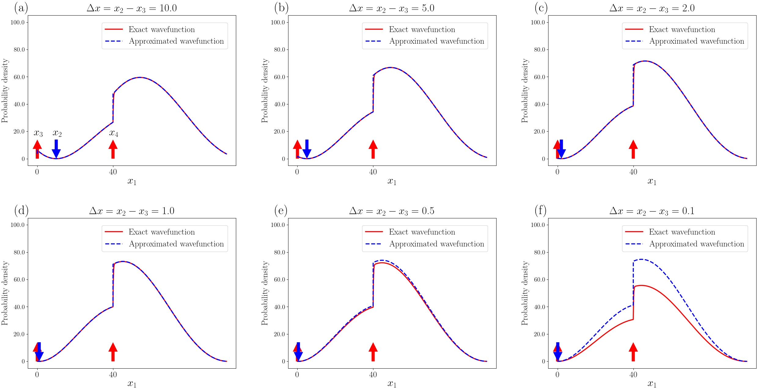
Figure 3: The probability distribution of four-particle wavefunction with $x_{2},x_{3},x_{4}$ fixed. From (a) to (f), we decrease the value of $x_{2}$, with $x_{3}=0$, $x_{4}=40$, $\Delta x=x_{2}-x_{3}$. Here we take $\chi_{1,2}=\chi_{3,4}=\pm 2\pi/L$, $m=1$, $g=1$, $\alpha=3$, $L=100$. The normalization of the original wavefunction and the approximated wavefunction differs by a ratio 0.00765. As a comparison, $\lambda_{s}/L=0.00333$.

Appendix B Solution to BA equation

We decouple the spin and momentum by applying a similar transformation $\hat{V}=\text{exp}(-m\alpha\sum_{l}\sigma^{z}_{l}x_{l})$. The wavefunction is converted to $\overline{\psi}_{\sigma}(x_{l})=\hat{V}\psi_{\sigma}(x_{l})$, where $\sigma$ denotes the spin components. Transformed Hamiltonian $\hat{\overline{H}}=\hat{V}\hat{H}\hat{V}^{-1}$ is

$$\hat{\overline{H}}=\sum_{l}-\frac{\nabla_{l}^{2}}{2m}+\sum_{\langle ll^{\prime}\rangle}2g\delta\left(x_{l}-x_{l^{\prime}}\right).$$

This transformation also twists the PBC to

$$\overline{\psi}_{\sigma}(x_{l})=e^{m\alpha L\sigma^{z}_{l}}\ \overline{\psi}_{\sigma}(x_{l}+L).$$

With this setup, the many-body problem can be solved using the BA method. The Bethe-type wave function is defined as

$$\overline{\psi}_{\sigma}\left(x_{l}\right)= \sum_{Q,P}\theta\left(x_{Q_{1}}>x_{Q_{2}}>\cdots>x_{Q_{N}}\right)$$ (25)

$$\times A_{\sigma}(Q,P)\ \exp\left(i\sum_{l}\overline{k}_{P_{l}}x_{Q_{l}}\right),$$

where $Q$ and $P$ represents permutations of the coordinates $\{x_{l}\}$ and momenta $\{\overline{k}_{l}\}$ respectively. $\sum_{Q,P}$ denotes a sum over all permutations. For eigenstates with $N_{\downarrow}$ and $N_{\uparrow}=N-N_{\downarrow}$ spin-down and spin-up particles, the corresponding BA equations are [39]

$$\prod_{i=1}^{N_{\downarrow}}\!\frac{\Lambda_{i}-\overline{k}_{l}-img}{\Lambda_{i}-\overline{k}_{l}+img}\!=\!e^{i\overline{k}_{l}L}e^{m\alpha L},$$ (26)

$$\prod_{l=1}^{N}\!\frac{\Lambda_{i}-\overline{k}_{l}-img}{\Lambda_{i}-\overline{k}_{l}+img}\!=\!-e^{2m\alpha L}\prod_{i^{\prime}=1}^{N_{\downarrow}}\!\frac{\Lambda_{i}-\Lambda_{i^{\prime}}-2img}{\Lambda_{i}-\Lambda_{i^{\prime}}+2img},$$

or equivalently

$$\prod_{j=1}^{N_{\uparrow}}\!\frac{\Gamma_{j}\!-\!\overline{k}_{l}-img}{\Gamma_{j}\!-\!\overline{k}_{l}+img}\!=\!e^{i\overline{k}_{l}L}e^{-m\alpha L},$$ (27)

$$\prod_{l=1}^{N}\!\frac{\Gamma_{j}\!-\!\overline{k}_{l}-img}{\Gamma_{j}\!-\!\overline{k}_{l}+img}\!=\!-e^{-2m\alpha L}\prod_{i^{\prime}=1}^{N_{\uparrow}}\!\frac{\Gamma_{j}\!-\!\Gamma_{j^{\prime}}-2img}{\Gamma_{j}\!-\!\Gamma_{j^{\prime}}+2img},$$

where $\Lambda_{i}$ and $\Gamma_{j}$ are the quasi-momenta of spin-down and up particles respectively. Eq. (26) and Eq. (27) yield the same solution to $\{\overline{k}_{l}\}$.

In what follows, BA equations will be solved in the case of $L\gg\lambda_{s}$. Let us examine the first set of equations in Eq. (26). Since $\Lambda_{i}-\overline{k}_{l}-img$ and $\Lambda_{i}-\overline{k}_{l}+img$ have the same magnitude, their quotient would not give an exponentially diverge factor $e^{L/\lambda_{s}}$, with two exceptions: (a) The denominator is nearly zero, i.e., $\Lambda_{i}-\overline{k}_{i}+img\sim e^{-L/\lambda_{s}}$. (b) $\text{exp}(i\overline{k}_{l}L)$ cancels with the divergence factor $e^{L/\lambda_{s}}$, implying that the leading order of $\mbox{Im}\overline{k}_{l}$ is $m\alpha$. Based on this observation, we propose the following trial solution

$$\begin{cases}\overline{k}_{i}=\Lambda_{i}+img-\epsilon_{i}e^{-2m\alpha L},&1\leq i\leqslant N_{\downarrow};\\ \overline{k}_{j}=\chi_{j}/L+i(m\alpha-\eta_{j}/L),&N_{\downarrow}+1\leq j\leqslant N,\end{cases}$$

where $\epsilon_{i}$, $\chi_{j}$ and $\eta_{j}$ are dimensionless real numbers. The same reasoning can be applied to Eq. (27), which yields another trial solution

$$\begin{cases}\overline{k}_{i}=\chi_{i}/L-i(m\alpha-\eta_{i}/L),&1\leq i\leqslant N_{\downarrow};\\ \overline{k}_{j}=\Gamma_{j}-img-\epsilon_{j}e^{-2m\alpha L},&N_{\downarrow}+1\leq j\leqslant N.\end{cases}$$

The two trial solutions should be consistent with each other. We combine the them into

$$\small\begin{cases}\overline{k}_{i}=\chi_{i}/L-i(m\alpha-\eta_{i}/L),\ \ &\Lambda_{i}=\overline{k}_{i}-img+\epsilon_{i}e^{-2m\alpha L};\\ \overline{k}_{j}=\chi_{j}/L+i(m\alpha-\eta_{j}/L),\ \ &\Gamma_{j}=\overline{k}_{j}+img+\epsilon_{j}e^{-2m\alpha L}.\end{cases}$$ (28)

By taking the trial solution Eq. (28) to BA equations Eq. (26) and Eq. (27) respectively, we obtain

$$\begin{cases}(1+g/\alpha)^{N_{\uparrow}}=e^{\eta_{i}}e^{i\chi_{i}};\\ (1+g/\alpha)^{N_{\downarrow}}=e^{\eta_{j}}e^{i\chi_{j}},\end{cases}$$ (29)

and

$$-\frac{2img}{\epsilon_{i}}\prod_{i^{\prime}\neq i}^{N_{\downarrow}}\frac{-2img}{\overline{k}_{i^{\prime}}-\overline{k}_{i}} =e^{-\eta_{i}}e^{i\chi_{i}},$$ (30)

$$\frac{\epsilon_{j}}{2img}\prod_{j^{\prime}\neq j}^{N_{\uparrow}}\frac{\overline{k}_{j^{\prime}}-\overline{k}_{j}}{2img} =e^{\eta_{j}}e^{i\chi_{j}},$$

which gives the following solution to $\{\overline{k}_{l}\}$:

$$\!\!\!\!\!\!\!\begin{cases}\overline{k}_{i}=2n_{i}\pi/L-i(m\alpha-N_{\uparrow}\eta_{r}/L);\\ \overline{k}_{j}=2n_{j}\pi/L+i(m\alpha-N_{\downarrow}\eta_{r}/L).\end{cases}$$ (31)

$\eta_{r}$ defined in Eq. (24) describes the localization strength of the two-body case. Note that the sub-leading order of $\text{Im}\overline{k}_{l}$ will scale with the density. To prevent it from exceeding the leading order term $m\alpha$, the following constraint should be proposed

$$\frac{N}{L}\ll\frac{m\alpha}{\ln(1+g/\alpha)},$$ (32)

which is the dilute limit claimed in the paper. We check our trial solution by taking it to the second set of equations in Eq. (26), which yields

$$-\frac{2img}{\epsilon_{i}}(1+g/\alpha)^{N_{\uparrow}}\prod_{i^{\prime}\neq i}^{N_{\downarrow}}\frac{2img}{\overline{k}_{i^{\prime}}-\overline{k}_{i}}=(-1)^{N_{\downarrow}-1}.$$

This equation matches the first equation in Eq. (30), confirming the correctness of the trial solution. The second equation in Eq. (30) can be recovered in parallel.

To determine the many-body wavefunction, we transform $\overline{\varphi}_{\sigma}\left(x_{l}\right)$ back to $\varphi_{\sigma}\left(x_{l}\right)$, where:

$$\varphi_{\sigma}\left(x_{l}\right)= \sum_{Q,P}\theta\left(x_{Q_{1}}>x_{Q_{2}}>\cdots>x_{Q_{N}}\right)$$ (33)

$$\times A_{\sigma}(Q,P)\ \exp\left(i\sum_{l}{k}_{P_{l},\sigma_{l}}x_{Q_{l}}\right).$$

In this expression, $k_{P_{l},\sigma_{l}}=\overline{k}_{P_{l}}-im\alpha\sigma_{l}$ with $\sigma_{l}=\uparrow,\downarrow$. Without loss of generality, we assume $\sigma_{i}=\downarrow$, $\sigma_{j}=\uparrow$ for any $1\leq i\leq N_{\downarrow}$, $N_{\downarrow}+1\leq j\leq N$. For a given permutation $\{P_{l}\}$ and $\{Q_{l}\}$, $\{k_{P_{l},\sigma_{l}}\}$ defines a scattering channel, where $1\leq P_{l}\leq N$. These scattering channels can be divided into two classes:

$$\text{Class (a):}\quad\exists\ l,\ \mbox{Im}\ k_{P_{l},\sigma_{l}} =\pm(2m\alpha-N_{\downarrow,\uparrow}\eta_{r}/L),$$

$$\text{Class (b):}\quad\forall\ l,\ \mbox{Im}\ k_{P_{l},\sigma_{l}} =\pm N_{\uparrow,\downarrow}\eta_{r}/L.$$

We will now prove that class (a) can be discarded in the dilute limit. For a channel in class (a), if the momentum of a spin-down particle satisfies $\mbox{Im}\ k_{P_{i},\sigma_{i}}=2m\alpha-N_{\uparrow}\eta_{r}/L$, there must exist a corresponding spin-up particle with momentum $\mbox{Im}\ k_{P_{j},\sigma_{j}}=-(2m\alpha-N_{\downarrow}\eta_{r}/L)$. Class (a) can have many such up-down pairs, each pair contributing an exponential factor $e^{2(x_{\uparrow}-x_{\downarrow})/\lambda_{s}}$. Depending on the coordinate permutation ($-L<x_{\uparrow}-x_{\downarrow}<0$ or $0<x_{\uparrow}-x_{\downarrow}<L$), this factor is either divergent or suppressed in the case of $L\gg\lambda_{s}$. If it diverges, the PBC can not be satisfied unless the corresponding scattering amplitude scales as $e^{-2L/\lambda_{s}}$. Therefore, regardless of whether the plane waves diverge or not, class (a) will always be suppressed by a factor $e^{-2x/\lambda_{s}}$ with $0<x<L$. An exception occurs when $x<\lambda_{s}$, which means a pair of spin-up and spin-down particles get very close to each other. However, in the dilute limit, the average distance between particles $L/N$ is much larger than $\lambda_{s}$, rendering the exceptional region negligible. Furthermore, scattering channels of class (a) will not accumulate to a finite value as $N\rightarrow\infty$. Although the number of these channels increase as $N!$, they are not coherent and will cancel out each other. To justify this argument, we numerically calculate the normalization of the approximated wavefunction and the exact wavefunction in the 4-particle case with 2 up-down pairs. They differ by a ratio of the magnitude $N\lambda_{s}/L$, which is roughly the normalization of a single channel in class (a).

In Fig. 3, we plot the probability distribution function $\left|\varphi_{\downarrow\downarrow\uparrow\uparrow}\left(x_{1},x_{2},x_{3},x_{4}\right)\right|^{2}$ with fixed $x_{2},x_{3},x_{4}$. The red line represents the exact wavefunction, while the blue line represents the approximated wavefunction. From figures (a) to (f), a pair of spin-up and spin-down particles get progressively closer to each other. In figures (a) to (d), the approximated probability distribution almost overlaps with the exact one. They only diverge in the vicinity of the spin-up particle at $x_{4}$, where the exact probability is smaller. This implies that the scattering channels of class (a) contribute a negative part to the probability, preventing an up-down pair getting too close. Such approximation breaks down when $x_{2}-x_{3}\sim\lambda_{s}$, as shown in figures (e) and (f). Nevertheless, the contribution to the normalization from the break-down region is negligible.

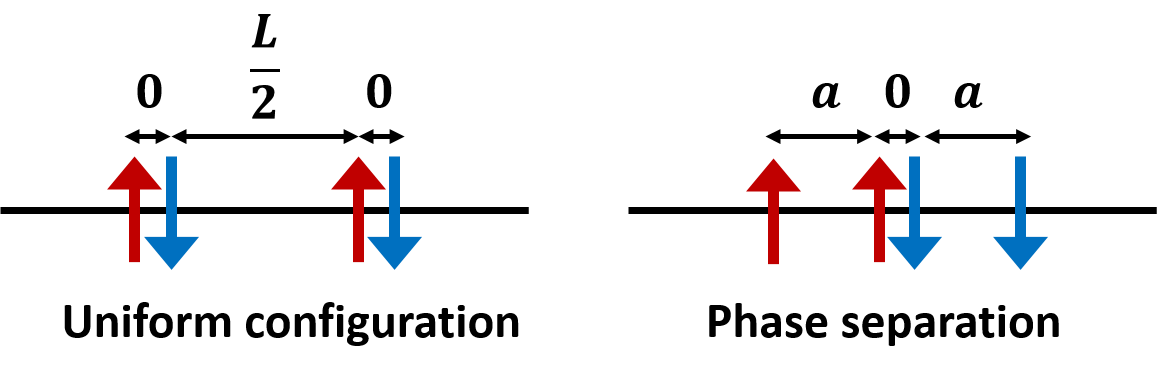
Figure 4: In the first configuration, four particles form two up-down pairs with distance $L/2$. The size of the pair is negligible; In the phase separation, particles with identical spins form two adjacent clusters with size $a=L\tan^{-1}(\frac{\pi}{2}\eta_{r})/\pi$.

With the reasoning above, all channels of class (a) can be discarded. In class (b), the solution Eq. (31) is written as:

$$\begin{cases}k_{i}=(2n_{i}\pi+iN_{\uparrow}\eta_{r})/L;\\ k_{j}=(2n_{j}\pi-iN_{\downarrow}\eta_{r})/L.\end{cases}$$ (34)

As we sum over all momentum permutations in the wavefunction Eq. (33), only those channels of class (b) should be included. For any fixed coordinate permutation, different channels in class (b) can transform to each other by reflection between particles with identical spins, and the corresponding phase shift is $-1$ due to Pauli’s exclusion principle. Consequently, these plane waves with momentum distribution Eq. (34) organize into a product of two Slater determinants for two spin components, simplifying the wavefunction to:

$$\varphi_{\sigma}\left(x_{l}\right)=\text{det}(e^{i\chi_{i_{1}}x_{i_{2}}/L})\text{det}(e^{i\chi_{j_{1}}x_{j_{2}}/L})e^{-\sum_{ij}\frac{1}{L}\eta_{r}(x_{i}-x_{j})}$$ (35)

$$\times\sum_{Q}\theta\left(x_{Q_{1}}>x_{Q_{2}}>\cdots>x_{Q_{N}}\right)A_{\sigma}(Q,Q)$$

$A_{\sigma}(Q,Q)$ denotes the scattering amplitude when the momentum permutation $P$ is identical to the coordinate permutation $Q$. To progress, we need to figure out the phase shift between these scattering amplitudes. Generally, $A_{\sigma}(Q,P)$ satisfies:

$$A_{\sigma}\left(Q,P\right)= \frac{\overline{k}_{P_{l+1}}-\overline{k}_{P_{l}}}{\overline{k}_{P_{l+1}}-\overline{k}_{P_{l}}+2img}A_{\sigma}\left(Q^{\prime},P^{\prime}\right)-$$ (36)

$$\frac{2img}{\overline{k}_{P_{i+1}}-\overline{k}_{P_{i}}+2img}A_{\sigma}\left(Q,P^{\prime}\right),$$

where

$$A_{\sigma}\left(Q^{\prime},P^{\prime}\right) =A_{\sigma}\left(\cdots Q_{l+1}Q_{l}\cdots,\cdots P_{l+1}P_{l}\cdots\right),$$

$$A_{\sigma}\left(Q,P^{\prime}\right) =A_{\sigma}\left(\cdots Q_{l}Q_{l+1}\cdots,\cdots P_{l+1}P_{l}\cdots\right).$$

Here $A_{\sigma}(Q,P)$, $A_{\sigma}(Q^{\prime},P^{\prime})$, $A_{\sigma}(Q,P^{\prime})$ represents the amplitudes of incident, transmission and reflection waves respectively. There are two cases to consider:

$$\text{(A): }1\leq Q_{l},\ Q_{l+1}\leq N_{\downarrow}\text{ or }N_{\downarrow}+1\leq Q_{l},\ Q_{l+1}\leq N$$

$$\text{(B): }1\leq Q_{l}\leq N_{\downarrow}\text{ and }N_{\downarrow}+1\leq\ Q_{l+1}\leq N$$

In case (A) $A_{\sigma}(Q,Q)=A_{\sigma}(Q^{\prime},Q^{\prime})$ due to the Fermi statistics. Case (B) represents the scattering between an up-down pair. According to Eq. (36)

$$A_{\sigma}\left(Q,Q\right)=\frac{1}{1+g/\alpha}A_{\sigma}\left(Q^{\prime},Q^{\prime}\right)-\frac{g/\alpha}{1+g/\alpha}A_{\sigma}\left(Q,Q^{\prime}\right),$$

where all the phase shifts are kept to the leading order. The reflection channel belongs to class (a), with the corresponding amplitude $A_{\sigma}(Q,Q^{\prime})\sim e^{-2L/\lambda_{s}}$, which vanishes in the dilute limit. Thus, we arrive at

$$\frac{A_{\sigma}(Q^{\prime},Q^{\prime})}{A_{\sigma}(Q,Q)}=1+\frac{g}{\alpha}=e^{\eta_{r}}.$$ (37)

Such phase shift applies to any up-down pair and is independent of the relative momentum between the pair. With this setup, the wavefunction Eq. (35) can be further simplified. First we define

$$\sum_{Q}\theta\left(x_{Q_{1}}<x_{Q_{2}}<\cdots<x_{Q_{N}}\right)A_{\sigma}(Q,Q)$$

$$=A_{\sigma}(x_{1},x_{2},\cdots x_{N})$$

with

$$A_{\sigma}(x_{1},x_{2},\cdots x_{N})=1$$

$$\text{if}\ \ x_{N_{\downarrow}+1}<x_{N_{\downarrow}+2}<\cdots<x_{N}<x_{1}<x_{2}<\cdots<x_{N_{\downarrow}}.$$

The function $A_{\sigma}(x_{1},x_{2},\cdots x_{N})$ is a constant for a given coordinate permutation. Its value changes only when the coordinates of an up-down pair switch. When all the spin-up particles are on the left side of spin-down particles, its value is defined as 1. According to the constant phase shift Eq. (37), every time a spin-up particle cross a spin-down particle from the left to the right, the value of $A_{\sigma}(x_{1},x_{2},\cdots x_{N})$ will multiply a factor $e^{-\eta_{r}}$. Therefore, we can use the following algorithm to determine the output of the function:

Step 1: Find all the positions of the spin-up particles

Step 2: For every spin-up particles, count how many spin-down particles staying on its left side. This number is denoted as $u_{j}$, where $j$ is the index of spin-up particles.

Step 3: Sum over $u_{j}$. The value of the function is given by $e^{-\eta_{r}\sum_{j}u_{j}}$.

$u_{j}$ can also be expressed as

$$u_{j}=\sum_{i}^{N_{\downarrow}}\theta(x_{j}-x_{i}).$$ (38)

In other words,

$$A_{\sigma}(x_{1},x_{2},\cdots x_{N})=e^{-\eta_{r}\sum_{ij}\theta(x_{j}-x_{i})},$$ (39)

which simplifies Eq. (35) to

$$\varphi_{\sigma}\left(x_{l}\right)=\text{det}(e^{i\chi_{i_{1}}x_{i_{2}}/L})\text{det}(e^{i\chi_{j_{1}}x_{j_{2}}/L})e^{-\frac{1}{2}\sum_{ij}\!W(x_{i}-x_{j})}.$$

This is the wavefunction shown in the main body of the paper.

Appendix C Phase transition in the four-particle case

In this section, we calculate the transition point for the system with two up-down pairs. The probability distribution function $\rho_{\beta}$ is defined as

$$\rho_{\beta}=e^{-\beta\mathcal{H}}.$$ (40)

In the zero-temperature limit $\beta\rightarrow\infty$, the system freezes into the state with minimal energy. For the four-particle case, $\mathcal{H}$ has two local minima, whose configurations are shown in Fig. 4. The energies of the uniform configuration $E_{1}$ and the phase separation $E_{2}$ are given by:

$$\left\{\begin{array}[]{l}E_{1}=2\eta_{r},\vspace{1ex}\\ E_{2}=\frac{8\eta_{r}a}{L}-4\ln(\sin\frac{\pi a}{L}).\vspace{1ex}\end{array}\right.$$ (43)

As a function of the cluster size $a$, $E_{2}$ is minimized when $a=L\tan^{-1}(\frac{\pi}{2}\eta_{r})/\pi$. The transition point is determined by setting $E_{1}=E_{2}$, which gives $\eta_{r}=3.84$. In the case of $\eta_{r}<3.84$ or $\eta_{r}>3.84$, $E_{1}$ or $E_{2}$ is the smaller one.

References

• Lee [2016] T. E. Lee, Anomalous edge state in a non-hermitian lattice, Phys. Rev. Lett. 116, 133903 (2016).
• Yao and Wang [2018] S. Yao and Z. Wang, Edge states and topological invariants of non-hermitian systems, Phys. Rev. Lett. 121, 086803 (2018).
• Lee et al. [2019] C. H. Lee, L. Li, and J. Gong, Hybrid higher-order skin-topological modes in nonreciprocal systems, Phys. Rev. Lett. 123, 016805 (2019).
• Lee and Thomale [2019] C. H. Lee and R. Thomale, Anatomy of skin modes and topology in non-hermitian systems, Phys. Rev. B 99, 201103 (2019).
• Borgnia et al. [2020] D. S. Borgnia, A. J. Kruchkov, and R.-J. Slager, Non-hermitian boundary modes and topology, Phys. Rev. Lett. 124, 056802 (2020).
• Kunst et al. [2018] F. K. Kunst, E. Edvardsson, J. C. Budich, and E. J. Bergholtz, Biorthogonal bulk-boundary correspondence in non-hermitian systems, Phys. Rev. Lett. 121, 026808 (2018).
• Yokomizo and Murakami [2019] K. Yokomizo and S. Murakami, Non-bloch band theory of non-hermitian systems, Phys. Rev. Lett. 123, 066404 (2019).
• Yang et al. [2020] Z. Yang, K. Zhang, C. Fang, and J. Hu, Non-hermitian bulk-boundary correspondence and auxiliary generalized brillouin zone theory, Phys. Rev. Lett. 125, 226402 (2020).
• Yao et al. [2018] S. Yao, F. Song, and Z. Wang, Non-hermitian chern bands, Phys. Rev. Lett. 121, 136802 (2018).
• Song et al. [2019] F. Song, S. Yao, and Z. Wang, Non-hermitian skin effect and chiral damping in open quantum systems, Phys. Rev. Lett. 123, 170401 (2019).
• Zhang et al. [2020] K. Zhang, Z. Yang, and C. Fang, Correspondence between winding numbers and skin modes in non-hermitian systems, Phys. Rev. Lett. 125, 126402 (2020).
• Brandenbourger et al. [2019] M. Brandenbourger, X. Locsin, E. Lerner, and C. Coulais, Non-reciprocal robotic metamaterials, Nature communications 10, 4608 (2019).
• Ghatak et al. [2020] A. Ghatak, M. Brandenbourger, J. Van Wezel, and C. Coulais, Observation of non-hermitian topology and its bulk–edge correspondence in an active mechanical metamaterial, Proceedings of the National Academy of Sciences 117, 29561 (2020).
• Xiao et al. [2020] L. Xiao, T. Deng, K. Wang, G. Zhu, Z. Wang, W. Yi, and P. Xue, Non-hermitian bulk–boundary correspondence in quantum dynamics, Nature Physics 16, 761 (2020).
• Hofmann et al. [2020] T. Hofmann, T. Helbig, F. Schindler, N. Salgo, M. Brzezińska, M. Greiter, T. Kiessling, D. Wolf, A. Vollhardt, A. Kabaši, C. H. Lee, A. Bilušić, R. Thomale, and T. Neupert, Reciprocal skin effect and its realization in a topolectrical circuit, Phys. Rev. Res. 2, 023265 (2020).
• Liu et al. [2021] S. Liu, R. Shao, S. Ma, L. Zhang, O. You, H. Wu, Y. J. Xiang, T. J. Cui, and S. Zhang, Non-hermitian skin effect in a non-hermitian electrical circuit, Research 2021 (2021).
• Zhang et al. [2021] L. Zhang, Y. Yang, Y. Ge, Y.-J. Guan, Q. Chen, Q. Yan, F. Chen, R. Xi, Y. Li, D. Jia, et al., Acoustic non-hermitian skin effect from twisted winding topology, Nature communications 12, 6297 (2021).
• Liang et al. [2022] Q. Liang, D. Xie, Z. Dong, H. Li, H. Li, B. Gadway, W. Yi, and B. Yan, Dynamic signatures of non-hermitian skin effect and topology in ultracold atoms, Phys. Rev. Lett. 129, 070401 (2022).
• Korepin et al. [1997] V. E. Korepin, V. E. Korepin, N. Bogoliubov, and A. Izergin, Quantum inverse scattering method and correlation functions, Vol. 3 (Cambridge university press, 1997).
• Wang et al. [2015] Y. Wang, W.-L. Yang, J. Cao, and K. Shi, Off-diagonal Bethe ansatz for exactly solvable models (Springer, 2015).
• Lieb and Liniger [1963] E. H. Lieb and W. Liniger, Exact analysis of an interacting bose gas. i. the general solution and the ground state, Phys. Rev. 130, 1605 (1963).
• Lieb [1963] E. H. Lieb, Exact analysis of an interacting bose gas. ii. the excitation spectrum, Phys. Rev. 130, 1616 (1963).
• Yang [1967] C. N. Yang, Some exact results for the many-body problem in one dimension with repulsive delta-function interaction, Phys. Rev. Lett. 19, 1312 (1967).
• Gaudin [1967] M. Gaudin, Un systeme a une dimension de fermions en interaction, Physics Letters A 24, 55 (1967).
• Lieb and Wu [1968] E. H. Lieb and F. Y. Wu, Absence of mott transition in an exact solution of the short-range, one-band model in one dimension, Phys. Rev. Lett. 20, 1445 (1968).
• Nakagawa et al. [2021] M. Nakagawa, N. Kawakami, and M. Ueda, Exact liouvillian spectrum of a one-dimensional dissipative hubbard model, Phys. Rev. Lett. 126, 110404 (2021).
• Mao et al. [2023] L. Mao, Y. Hao, and L. Pan, Non-hermitian skin effect in a one-dimensional interacting bose gas, Phys. Rev. A 107, 043315 (2023).
• Wang et al. [2023] H.-R. Wang, B. Li, F. Song, and Z. Wang, Scale-free non-Hermitian skin effect in a boundary-dissipated spin chain, SciPost Phys. 15, 191 (2023).
• Kattel et al. [2023] P. Kattel, P. R. Pasnoori, and N. Andrei, Exact solution of a non-hermitian pt-symmetric spin chain, Journal of Physics A: Mathematical and Theoretical 56, 325001 (2023).
• Zheng et al. [2024] M. Zheng, Y. Qiao, Y. Wang, J. Cao, and S. Chen, Exact solution of the bose-hubbard model with unidirectional hopping, Phys. Rev. Lett. 132, 086502 (2024).
• Ogata and Shiba [1990] M. Ogata and H. Shiba, Bethe-ansatz wave function, momentum distribution, and spin correlation in the one-dimensional strongly correlated hubbard model, Phys. Rev. B 41, 2326 (1990).
• Laughlin [1983] R. B. Laughlin, Anomalous quantum hall effect: An incompressible quantum fluid with fractionally charged excitations, Phys. Rev. Lett. 50, 1395 (1983).
• Yang et al. [2019] W. Yang, J. Wu, S. Xu, Z. Wang, and C. Wu, One-dimensional quantum spin dynamics of bethe string states, Phys. Rev. B 100, 184406 (2019).
• Wang et al. [2018] Z. Wang, J. Wu, W. Yang, A. K. Bera, D. Kamenskyi, A. N. Islam, S. Xu, J. M. Law, B. Lake, C. Wu, et al., Experimental observation of bethe strings, Nature 554, 219 (2018).
• Takahashi [1999] M. Takahashi, Thermodynamics of One-Dimensional Solvable Models (Cambridge University Press, 1999).
• Jastrow [1955] R. Jastrow, Many-body problem with strong forces, Phys. Rev. 98, 1479 (1955).
• Li et al. [2020] L. Li, C. H. Lee, S. Mu, and J. Gong, Critical non-hermitian skin effect, Nature communications 11, 5491 (2020).
• Li et al. [2021] L. Li, C. H. Lee, and J. Gong, Impurity induced scale-free localization, Communications Physics 4, 42 (2021).
• Zvyagin and Schlottmann [2013] A. A. Zvyagin and P. Schlottmann, Effects of spin-orbit interaction in the hubbard chain with attractive interaction: Application to confined ultracold fermions, Phys. Rev. B 88, 205127 (2013).
• Gros et al. [1987] C. Gros, R. Joynt, and T. M. Rice, Antiferromagnetic correlations in almost-localized fermi liquids, Phys. Rev. B 36, 381 (1987).
• Yi and Yang [2020] Y. Yi and Z. Yang, Non-hermitian skin modes induced by on-site dissipations and chiral tunneling effect, Phys. Rev. Lett. 125, 186802 (2020).