Estimation of service value parameters for a queue with unobserved balking

Abstract

In Naor’s model [16], customers decide whether or not to join a queue after observing its length. We suppose that customers are heterogeneous in their service value (reward) $R$ from completed service and homogeneous in the cost of staying in the system per unit of time. It is assumed that the values of customers are independent random variables generated from a common parametric distribution. The manager observes the queue length process, but not the balking customers. Based on the queue length data, an MLE is constructed for the underlying parameters of $R$. We provide verifiable conditions for which the estimator is consistent and asymptotically normal. A dynamic pricing scheme is constructed that starts from some arbitrary price and iteratively updates the price using the estimated parameters. The performance of the estimator and the pricing algorithm are studied through a series of simulation experiments.

1 Introduction

Economic models for congested service systems include various population parameters that influence the demand and, consequently, optimal admission pricing. Two key parameters are the value of goods or services to the individual and their sensitivity to waiting time. These factors influence the amount of time an individual is willing to wait in a queue. These factors are often unknown to the system administrator. Furthermore, customers often have heterogeneous values, a feature that can be modeled as a probability distribution within the population. By assuming parametric distributions, one can estimate the parameters from data such as queue states, service times, and interarrival times. These estimators can be further used to answer questions of optimal design and control. For example, a revenue-maximizing admission price can be determined based on the estimated parameters. Another common objective is social welfare maximization, which also requires understanding the underlying utility parameters of the customers. Government and non-profit organizations may be interested in improving the quality of their services, such as subsidized meal centers. This can be achieved with a social welfare-maximizing price. Conversely, a restaurant owner may be interested in profit maximization.

In the current work, we consider a variant of Naor’s model (see [16]), where the service value of customers is a random variable $R$ following a parametric distribution $F_{\theta}$. The queue is observable, so some customers balk when the queue is too long, considering their individual service value. The balking threshold is random and depends on the distribution of $R$. The effective queue length process is monitored by a system administrator, meaning balking customers are not observed. Based on this information, a maximum likelihood estimator (MLE) for the parameters of the service value distribution is constructed. The asymptotic performance of this estimator is studied under certain assumptions about the parametric class of service value distributions. The MLE is then used to construct an iterative price optimization algorithm for revenue maximization.

1.1 Statistical model and objective

Customers arrive at a single first-come-first-served (FCFS) queue according to a stationary Poisson process with rate $\lambda$. The service times are independently, identically, and exponentially distributed with parameter $\mu$. Customers are heterogeneous and strategically decide whether to join or balk after observing the queue length. In Naor’s model (see [16], [15] and[11]), a customer’s benefit from completed service is $R$. The cost to a customer for staying in the system (either while waiting or being served) is $C$ per unit of time spent in the system (sojourn+service time). The system charges an admission price $p$ from every joining customers. Customers are risk-neutral, meaning they maximize the expected value of their net benefit. From a public (social) point of view, the utility functions of individual customers are identical and additive. Thus, given a value $R$, every customer has an individual optimal threshold strategy that dictates whether to join or balk at the observed queue length. A decision to join is irrevocable, and reneging is not allowed. A customer who balks leaves the system and never returns. The service values of customers are iid with a common random variable $R\sim F_{\theta}$, where $F_{\theta}$ is a cumulative distribution function (cdf) and $\theta\in\mathbb{R}^{d}$ is a parameter that fully determines the distribution (see [15]). We further assume that $C$ is fixed and known by all customers and the system administrator.

For an admission price $p$, a customer with service value $R$ that, observes a queue of length $q$ upon arrival, joins the queue if the expected utility is non-negative; $R-p-\frac{C(q+1)}{\mu}>0$. In other words, the customer joins the queue if the benefit $R-p$ is higher than the total expected time in the system multiplied by C, i.e., if $R-p\geq\frac{(q+1)C}{\mu}$. It is easy to show (see [16]) that the customer balks if he observes $n_{e}=\lfloor\frac{(R-p)\mu}{C}\rfloor$ where $\lfloor x\rfloor$ is the floor function. The probability of this event is $1-F_{\theta}(p+\frac{(q+1)C}{\mu})$. Thus, the joining process is not Poisson with rate $\lambda$, but rather a Poisson process with state-dependent rates;

$$\lambda_{q}=\lambda\mathrm{P}\left(R\geq p+\frac{(q+1)C}{\mu}\right)=\lambda\left(1-F_{\theta}\left(p+\frac{(q+1)C}{\mu}\right)\right)\ ,q=0,1,2,\ldots\ .$$

We denote the arrival probability at state $q$ by $\mathrm{P}_{q}=1-F\left(p+\frac{(q+1)C}{\mu}\right)$, and illustrate the transition diagram of the underlying CTMC in Figure 1.

Figure 1: Transition diagram of a queue with Poisson arrival process with state dependent rate $\lambda_{q}$ and exponential service rate $\mu$.

The available data is the queue-length process: $(Q_{0},\ldots,Q_{k})$, where $Q_{0}$ is an initial state and $k$ is the sample size (or number of transitions). This implies that the customers who balk are not observed; consequently, this information cannot be used. This yields an interesting trade-off between revenue maximization and statistical inference. Namely, a system with a higher admission price will have a lower joining rate (at every system state), and so the data collection for inference purposes will be slower. Thus, the price can be reduced to learn faster and obtain the optimal price. However, too low a price will considerably reduce the profit. In Naor’s model, for a fixed reward, it is typically assumed that $R\mu\geq C$, so that customers always join an empty queue. We replace this assumption with $\mathrm{P}(R\geq C/\mu)=F_{\theta}(C/\mu)>0$. Therefore, when the queue is empty, there is a positive probability that a customer will join the queue. Otherwise, the queue is always empty and there is no information for inference.

In this work, a maximum likelihood estimator for $\theta$ is derived and analyzed. There is no way to directly observe realizations of $R$; however, the queue that can be observed contains information about it. Thus, assuming that the cost of staying in the system per unit of time $C$ is constant, our first goal is to estimate the parameters of $R$ using queue information. The second goal is to suggest an iterative dynamic pricing algorithm for revenue maximization.

1.2 Outline and contribution

• In Section 2 we develop an MLE for the parameters of the service value distribution.

• In Section 3 we show that under standard regularity assumptions, the MLE is consistent and the normalized errors are asymptotically normally distributed. A formula for the asymptotic variance is further derived in terms of $F$ and the corresponding stationary distribution of the queue-length.

• In Section 4 we propose an iterative data-driven pricing algorithm. Assuming a specific distribution of $R$ some arbitrary price can be chosen and queue data can be collected. This data can be used to estimate the underlying parameters of $R$ distribution, and to choose a better price. The repetition of the procedure leads to the optimal price (or close enough to it).

• In Section 5 we assume that $R$ is exponentially distributed. We verify that all assumptions hold and illustrate the asymptotic behavior of the estimator via simulation experiments. In addition, we apply the algorithm proposed in Section 4 to the exponential case. The algorithm is shown to converge quickly to the revenue maximizing price.

• Section 6 provides concluding remarks and discusses several possible extensions of the method.

1.3 Literature review

The first model that proposed quantitative analysis of an entrance fee (price) in queueing models with economic parameters was Naor’s model [16]. The model analyzed optimal pricing for profit and social welfare maximization for the FCFS $M/M/1$ queueing model. In Naor’s settings, the arriving customer observes the queue length and decides whether they want to join the queue or balk. The decision is based on $C$ - the cost of staying in the system per unit of time, and the benefit gained from the completed service $R$ and $\mu$ - the service rate. As stated above, the individually optimal joining threshold is given by $n_{e}=\lfloor\frac{(R-p)\mu}{C}\rfloor$. Naor further characterized the socially optimal threshold $n^{*}$ and the monopolistic (profit-maximizing) threshold $n_{m}$. In particular, he showed that $n_{m}\leq n^{*}\leq n_{e}$, where the total social welfare is maximized under the assumption that individual benefits are additive. Customers can be ‘forced’ to join according to the optimal thresholds by charging an admission fee (can be interpreted as service price) $p$, or an increase of the cost per unit of time $C$ (see [11]). The price can be decided on in different ways.

Naor’s model was extended in [15] to allow for heterogeneous service values. In this case, $R$ is assumed to be a continuous, non-negative random variable, and then the underlying process is an M/M/1 with state-dependent joining rates (see Figure 1). [15] derived, numerically, the socially and monopoly optimal prices for $R\sim U(a,b)$. It is further shown that the profit-maximizing fee is larger or equal to the fee that optimizes social welfare. However, this property does not necessarily hold if customers differ by their waiting time sensitivity (see [11]). Schroeter made a generalization in a different direction. He assumed $C\sim U(0,b)$ and derived the profit-maximizing price. A customer observing a queue of length $q_{i}$, upon arrival, joins the queue if $C\leq\frac{(R-p)\mu}{q_{i}+1}$. Under some assumptions, Schroeter found that the profit-maximizing price admits a closed form solution. The question of maximizing social welfare and revenue for systems with heterogeneous customers has since been addressed in many studies with various model assumptions, and we refer the reader to [10] for an in-depth review of these results.

There is a broad literature dealing with parameter and state estimation for queueing systems, which has recently been surveyed in [3]. This literature focuses mostly on estimating the features of the queue, such as queue states, arrival and service rates, workload, idle times, and so on. In other words, the parameters of the queue itself. To the best of our knowledge, only a few works have concentrated on studying the customers’ economic characteristics through the queuing process. One such work is [18], which proposes an estimator for delay and tardiness sensitivities in a queue with strategic timing of arrivals. They show that the estimator is strongly consistent, and the normalized errors are asymptotically normal with a known covariance matrix. The estimator is constructed using the method of moments from the Wardrop equilibrium condition. There is a stream of literature that considers the problem of estimating customer patience for service systems with abandonments (e.g., [2]). Note that the current work is also related to the classical statistical problem of asymptotic performance of maximum likelihood estimators of parameters of Markov chains and Birth-death processes in particular (e.g., [4] and [21]).

In the context of systems with unobserved balking, [13] deals with the maximum likelihood estimation of customer patience parameters based on effective inter-arrival time data. They assume customers have a random continuous patience level and will join the queue only if the delay is below this level. Note that this does not necessarily assume a utility-based decision as in Naor’s model. Their method involves deriving a maximum likelihood estimator (MLE) based on observations of effective inter-arrival times. Strong consistency of the MLE and the asymptotic distribution of the estimation error, which is not always normal, are derived. This approach has been extended to a multi-server non-homogeneous in time arrival process in [5]. A closely related problem is that of admission pricing in the presence of uncertainty regarding customer parameters. For example, in Naor’s model, [1] assume an identical reward and two types of customers: patient customers with a low waiting cost $c_{L}$, and impatient customers with a high waiting cost $c_{H}$. They propose a Bayesian dynamic pricing model (queue-length dependent) to estimate the proportion of patient customers and establish convergence to the optimal pricing policy. In [7], an online stochastic approximation algorithm is presented for the problem of jointly setting an admission price and capacity allocation. This is done for a G/G/1 queue where the incoming arrival rate is a function of the admission price, but not of the real-time congestion levels. Under mild assumptions the algorithm is shown to converge to the optimal policy. A final related work is [17] that presents a stochastic approximation algorithm that estimates the Nash equilibrium (rather than system optimal) strategy for a general class of queueing games.

2 Maximum likelihood estimator for $\boldsymbol{\theta}$

Assume that customers arrive at a single server facility according to a Poisson process with rate $\lambda$. The service times are independently, identically, and exponentially distributed with parameter $\mu$. Upon arrival, customers see a queue length $q_{i}$ and a fixed admission price $p$. Assume that the customers are homogeneous in their waiting time sensitivity, i.e., $C$ is constant, and that this value is known. Also, $R$ is a RV with some CDF $F(r,\boldsymbol{\theta})$. For the sake of brevity, we simplify $F(r,\boldsymbol{\theta})$ to $F(r)$, however, the reader should keep in mind that $F$ does depend on $\boldsymbol{\theta}$. In addition, as was previously mentioned, we assume that there is a positive probability that a customer joins an empty queue; $F(C/\mu,\boldsymbol{\theta})>0$.

The queue-length process is clearly a continuous-time Markov chain (specifically, a birth-death process) on the non-negative integers, with state dependent transition rates. Throughout this work we consider the underlying discrete-time jump chain. We refer to a transition in the queue state as a “step”, and the initial state of the system is the queue length in step $0$ - before the first jump. Thus, the system state at step $i$ is the queue length after $i$ jumps. Let $Q_{i}$ denote the state at step $i\geq 0$,. Given $Q_{i-1}=q_{i-1}$), applying the Markov property, the probability that in step $i$ the queue length ($Q_{i}$) goes up by one is

$$\mathrm{P}(Q_{i}=q_{i-1}+1|Q_{i-1}=q_{i-1})=\left\{\begin{matrix}1&,\>\>q_{i-1}=0\\ \frac{\lambda_{i}}{\lambda_{i}+\mu}&,\>\>q_{i-1}>0\end{matrix}\right.\;,$$

where

$$\lambda_{i}:=\lambda\left(1-F\left(p+\frac{C(q_{i-1}+1)}{\mu}\right)\right)\;\;.$$

Similarly,

$$\mathrm{P}(Q_{i}=q_{i-1}-1|Q_{i-1}=q_{i-1})=\left\{\begin{matrix}0&,\>\>q_{i-1}=0\\ \frac{\mu}{\lambda_{i}+\mu}&,\>\>q_{i-1}>0\end{matrix}\right.\;.$$

For the sake of a compact representation, let $r(q_{i})=p+\frac{(q_{i}+1)C}{\mu}$. Iterating the Markov property, the probability to see a path $q_{k},q_{k-1},q_{k-2},...,q_{0}$, for a given parameter $\boldsymbol{\theta}$, is

$$\mathrm{P}(Q_{k}=q_{k},Q_{k-1}=q_{k-1},Q_{k-2}=q_{k-2},...,Q_{0}=q_{0},\boldsymbol{\theta})=\prod_{i=1}^{k}\mathrm{P}(Q_{i}=q_{i}|Q_{i-1}=q_{i-1},\boldsymbol{\theta})$$

$$\ =\prod_{i\in K_{1}}\mathrm{P}(Q_{i}=q_{i-1}+1|Q_{i-1}=q_{i-1},\boldsymbol{\theta})\prod_{i\in K_{2}}\mathrm{P}(Q_{i}=q_{i-1}-1|Q_{i-1}=q_{i-1},\boldsymbol{\theta})\prod_{i\in K_{3}}1,$$

where $K_{1}=\{1\leq i\leq k\>|\>Q_{i}=q_{i-1}+1,q_{i-1}\neq 0\}$, $K_{2}=\{1\leq i\leq k\>|\>Q_{i}=q_{i-1}-1,\>F(r(q_{i-1}))\neq 1\}$ and $K_{3}=\{1\leq i\leq k\>|\>F(r(q_{i-1}))\in\left\{0,1\right\}\}$. $K_{3}$ is a group of indices where the probability of upward or downward transition is $1$. $\mathrm{P}(Q_{i}=q_{i-1}+1|Q_{i-1}=q_{i-1})=1$ when $F(r(q_{i-1}))=0$ and $\mathrm{P}(Q_{i}=q_{i-1}-1|Q_{i-1}=q_{i-1})=1$ when $F(r(q_{i-1}))=1$. Thus, this likelihood can be rewritten as

$$\mathcal{L}(\boldsymbol{\theta}|Q_{k}):=\prod_{i\in K_{1}}\frac{\lambda(1-F(r(q_{i-1}),\boldsymbol{\theta}))}{\mu+\lambda(1-F(r(q_{i-1}),\boldsymbol{\theta}))}\prod_{i\in K_{2}}\frac{\mu}{\mu+\lambda(1-F(r(q_{i-1}),\boldsymbol{\theta}))}\prod_{i\in K_{3}}1\;\;.$$

Thus, after $k$ steps, the log-likelihood of $\boldsymbol{\theta}$ is:

$$\log\mathcal{L}(\boldsymbol{\theta}|Q_{k}) =\log\left\{\Pi_{i\in K_{1}}\frac{\lambda(1-F(r(q_{i-1}),\boldsymbol{\theta}))}{\mu+\lambda(1-F(r(q_{i-1}),\boldsymbol{\theta}))}\Pi_{i\in K_{2}}\frac{\mu}{\mu+\lambda(1-F(r(q_{i-1}),\boldsymbol{\theta}))}\Pi_{i\in K_{3}}1\right\}$$

$$\ =-\sum_{i\in K_{1}\cup K_{2}}\log\left\{\mu+\lambda\left(1-F(r(q_{i-1}),\boldsymbol{\theta})\right)\right\}+\sum_{i\in K_{1}}\log\left\{\lambda(1-F\left(r(q_{i-1}),\boldsymbol{\theta})\right)\right\}+|K_{2}|\log\left\{\mu\right\}\;,$$

where $|K_{2}|$ is the cardinality of $K_{2}$.

The Maximum Likelihood Estimator (MLE) is the solution of the optimization problem

$$\hat{\boldsymbol{\theta}}_{k}=\underset{\boldsymbol{\theta}\in\boldsymbol{\Theta}}{\text{argmax}}\left\{\log\mathcal{L}(\boldsymbol{\theta}|Q_{k})\right\},$$

where $\boldsymbol{\Theta}\subset\mathbb{R}^{n}$ is the parameter space. If the solution is interior, it can be derived with the first-order condition

$$\nabla\log\mathcal{L}(\boldsymbol{\theta}|Q_{k})=\boldsymbol{0},$$

where $\nabla\log\mathcal{L}(\boldsymbol{\theta}|Q_{k})$ is a vector-valued gradient $\mathbb{R}^{n}\rightarrow\mathbb{R}^{n}$ of log-likelihood function. Or, in more detail,

$$\begin{matrix}\frac{\partial\log\mathcal{L}(\theta_{j}|Q_{k})}{\partial\theta_{j}}=\sum_{i\in K_{1}\cup K_{2}}\left(\frac{\lambda F_{\theta_{j}}^{\prime}(r(q_{i-1}),\boldsymbol{\theta})}{\mu+\lambda(1-F(r(q_{i-1}),\boldsymbol{\theta}))}\right)-\sum_{i\in K_{1}}\left(\frac{\lambda F_{\theta_{j}}^{\prime}(r(q_{i-1}),\boldsymbol{\theta})}{\lambda(1-F(r(q_{i-1}),\boldsymbol{\theta}))}\right)=0\;,\\ \\ \forall j=1.\ldots,n\end{matrix}$$

where $F_{\theta_{j}}^{\prime}=\frac{\partial F}{\partial\theta_{j}}$. Otherwise, it lies on the boundary of $\boldsymbol{\Theta}$. In addition to $Q_{k}$ as defined previously, we denote the random variable $\mathbf{Y}_{k}=(Y_{1},Y_{2},...,Y_{k})$ where $Y_{i}$ is indicator of an upward transition $Y_{i}=1(Q_{i}>Q_{i-1})$. Thus, conditional on $Q_{i-1}=q_{i-1}$,

$$Y_{i}\sim Ber(p(q_{i-1},\boldsymbol{\theta})),$$

where $p(q_{i-1},\boldsymbol{\theta}):=\mathrm{P}(Q_{i}=q_{i-1}+1|Q_{i-1}=q_{i-1})$. In addition, we introduce $M:=K_{1}\cup K_{2}=K\backslash K_{3}$. The set $M$ of indexes $i$ , is the set of indexes where $F(r(q_{i-1}),\boldsymbol{\theta})\notin\left\{0,1\right\}$, formally: $M=\{1\leq i\leq k\>|\>F(r(q_{i-1}),\boldsymbol{\theta})\notin\left\{0,1\right\}\}$. $M$ can be thought as effective sample and $|M|$ as effective sample size, while $K$ is the full sample and $|K|=k$ is the full sample size.

For any $q$ such that $F(r(q_{i-1}),\boldsymbol{\theta})\in\left\{0,1\right\}$, $p(q_{i-1},\boldsymbol{\theta})\in\left\{1,0\right\}$, so $\frac{\partial p(0,\theta_{j})}{\partial\theta_{j}}=0$, $\forall j\in n$. This case does not add any information to the likelihood function or its derivative. Thus, to simplify further notions, we ignore this case and consider only the sample of observations with indices in $M$. It is important to note that it does not affect assumptions and results. Observe that $p(q_{i-1},\theta)=\frac{\lambda_{i}}{\lambda_{i}+\mu}$ for any $i\in M$. Then, the log-likelihood can be rewritten as

$$\log\mathcal{L}(\boldsymbol{\theta}|Q_{k},Y_{k})=\frac{1}{k}\sum_{i\in M}[Y_{i}\log\left\{p(Q_{i-1},\boldsymbol{\theta})\right\}+(1-Y_{i})\log\left\{1-p(Q_{i-1},\boldsymbol{\theta})\right\}].$$

The gradient is given by

$$\nabla\log\mathcal{L}(\boldsymbol{\theta}|Q_{k},Y_{k}):=\boldsymbol{\Psi}_{k}(\boldsymbol{\theta})=\frac{1}{k}\sum_{i\in M}\boldsymbol{\psi}(Q_{i-1},Y_{i},\boldsymbol{\theta})$$

where

$$\boldsymbol{\psi}(Q_{i-1},Y_{i},\boldsymbol{\theta})=\begin{bmatrix}\psi^{1}(Q_{i-1},Y_{i},\boldsymbol{\theta})\\ \\ \vdots\\ \\ \psi^{n}(Q_{i-1},Y_{i},\boldsymbol{\theta})\end{bmatrix}=\begin{bmatrix}Y_{i}\frac{p^{\prime}_{\theta_{1}}(Q_{i-1},\boldsymbol{\theta})}{p(Q_{i-1},\boldsymbol{\theta})}-(1-Y_{i})\frac{p^{\prime}_{\theta_{1}}(Q_{i-1},\boldsymbol{\theta})}{1-p(Q_{i-1},\boldsymbol{\theta})}\\ \\ \vdots\\ \\ Y_{i}\frac{p^{\prime}_{\theta_{n}}(Q_{i-1},\boldsymbol{\theta})}{p(Q_{i-1},\boldsymbol{\theta})}-(1-Y_{i})\frac{p^{\prime}_{\theta_{n}}(Q_{i-1},\boldsymbol{\theta})}{1-p(Q_{i-1},\boldsymbol{\theta})}\end{bmatrix}$$

3 Asymptotic properties.

The fact that customers are less likely to join as the queue grows, i.e., $1-F(r)\to 0$ as $r\to\infty$, ensures that the queue-length process is stable. Formally, we will later assert that the sequence $(Q_{i-1},Y_{i})$ converges to a stationary distribution. We will assume throughout that the initial state follows the stationary distribution, hence the stationary random vector is represented by $(Q_{0},Y_{1})$. The ergodic limit of the gradient with respect to the parameter, if it exists, is denoted by $\boldsymbol{\Psi}$;

$$\boldsymbol{\Psi}_{k}(\boldsymbol{\theta})\overset{a.s.}{\longrightarrow}\boldsymbol{\Psi}(\boldsymbol{\theta})\ ,\boldsymbol{\theta}\in\Theta.$$

We next present sufficient conditions for consistency of the MLE, and for asymptotic normality of the estimation errors. Note that we use $||\cdot||$ for the euclidean distance of vectors in $\mathbb{R}^{n}$, and $|\cdot|$ for a vector of absolute values of their coordinates. For a matrix $\mathbf{A}$, its transpose is denoted by $\mathbf{A}^{T}$ and its inverse by $\mathbf{A}^{-1}$.

Assumptions

A1. $\boldsymbol{\Theta}$ is a compact and convex set and $\boldsymbol{\theta}_{0}$ is an interior point in $\boldsymbol{\Theta}$.

A2. $F(r,\boldsymbol{\theta})$ is continuous w.r.t. $\boldsymbol{\theta}\in\boldsymbol{\Theta}$. Furthermore, the gradient $\nabla F$ is also continuous and differentiable w.r.t. $\boldsymbol{\theta}\in\boldsymbol{\Theta}$.

A3. There exists a real valued function $H:\mathbb{N}\to\mathbb{R}$ such that

$$\max_{j=1,\ldots,n}\left|\frac{\nabla F(r(q),\boldsymbol{\theta})}{1-F(r(q),\boldsymbol{\theta})}\right|_{j}\leq H(q)\ ,\forall q\geq 0,$$

and $\mathbb{E}[H(Q_{0})]<\infty$.

A4. For any $j,l\in\{1,\ldots,n\}$, let

$$\Sigma_{jl}:=\mathbb{E}\left[\frac{\mu\lambda F^{\prime}_{\theta_{j}}(r(Q_{0}),\boldsymbol{\theta}_{0})F^{\prime}_{\theta_{l}}(r(Q_{0}),\boldsymbol{\theta}_{0})}{(1-F(r(Q_{0}),\boldsymbol{\theta}_{0}))(\mu+\lambda(1-F(r(Q_{0}),\boldsymbol{\theta}_{0})))^{2}}\right].$$

The matrix $\boldsymbol{\Sigma}$ is invertible and $|\Sigma_{jl}|<\infty$ for any $j,l\in\{1,\ldots,n\}$.

Our asymptotic results rely on the framework of [19] and the assumptions are standard in statistical theory. The main modification is that we are dealing with indirect estimation. In particular, the data is not an iid sample of service value observations, but rather the Markov chain $(Q_{i-1},Y_{i})$ whose transition matrix is determined by the service value distribution. For consistency the main idea is to ensure that $\boldsymbol{\psi}(Q_{i-1},Y_{i},\boldsymbol{\theta})$ converges uniformly to a “well-behaved” theoretical score function that has a unique root at the true parameter value. Assumptions A1, and A2 are used to establish continuity of $\boldsymbol{\psi}(q,y,\boldsymbol{\theta})$ and its first two derivatives w.r.t. $\boldsymbol{\theta}$. In addition, in order to show that MLE is consistent we must assume that $\boldsymbol{\theta}_{0}$ is an interior point of the parameter space (A1). If $\boldsymbol{\theta}_{0}$ lies on the boundary of $\boldsymbol{\Theta}$ the convergence to the true value is not guaranteed and the limiting distribution of the error may not be normal. Assumption A3 will be used to construct a uniform bound on $\boldsymbol{\psi}$ that is integrable with respect to the stationary distribution, which together with A1,A2 implies uniform convergence of $\boldsymbol{\Psi}_{k}(\boldsymbol{\theta})$ on $\boldsymbol{\Theta}$. The last assumption (A4) is used to show that the stationary variance of the estimation error exists and is finite. This will be used to verify a martingale CLT implying that the estimation errors are normally distributed.

Perhaps the only non-standard assumptions here that arise from the special structure of the process is A3 and A4. To gain some additional intuition for these condition, $1-F(r(q),\boldsymbol{\theta})$ can be thought as balking rate, while $\nabla_{\boldsymbol{\theta}}F(r(q),\boldsymbol{\theta})$ is gradient of $F(r(q),\boldsymbol{\theta})$ w.r.t. $\boldsymbol{\theta}$. It converges to the true value as number of observations grows. However, if the balking rate grows too fast as $q\rightarrow\infty$, the effective sample can be too small. Note, however, that this is a sufficient but not necessary condition. In Section 5.2 these conditions are verified for the special case of exponentially distributed $R$.

3.1 Consistency.

Theorem 1.

Under Assumptions A1, A2, A3, the MLE is consistent; $\hat{\boldsymbol{\theta}}_{k}\overset{p}{\rightarrow}\boldsymbol{\theta}_{0}$ as $k\rightarrow\infty$.

Proof.

To show consistency we verify the sufficient conditions given in [19, Thm. 5.9]. In particular, we need to show that

$$\inf_{\boldsymbol{\theta}:d(\boldsymbol{\theta},\boldsymbol{\theta}_{0})\geq\epsilon}||\boldsymbol{\Psi}(\boldsymbol{\theta})||>0=||\boldsymbol{\Psi}(\boldsymbol{\theta}_{0})||,$$ (1)

and that the class of functions $\{\boldsymbol{\Psi}_{k}(\boldsymbol{\theta}):\ \boldsymbol{\theta}\in\boldsymbol{\Theta}\}$ is Glinvenko-Cantelli (in the strong sense);

$$\sup_{\boldsymbol{\theta}\in\boldsymbol{\Theta}}\left|\left|\boldsymbol{\Psi}_{k}(\boldsymbol{\boldsymbol{\theta}})-\boldsymbol{\Psi}(\boldsymbol{\boldsymbol{\theta}})\right|\right|\overset{\mathrm{a.s.}}{\longrightarrow}0.$$ (2)

Then, by [19, Thm. 5.9], any sequence of estimators such that

$$\boldsymbol{\Psi}_{k}(\hat{\boldsymbol{\theta}}_{k})\overset{P}{\longrightarrow}\boldsymbol{0},$$ (3)

is consistent. The proof relies on a sequence of lemmas. First of all, Lemma 1 establishes the continuity of $\boldsymbol{\psi}$ under Assumption A2. Lemma 2 shows that $\boldsymbol{\psi}$ is bounded by the integrable function $H$ in Assumption A3 (up to a multiplicative constant). Note that we are only interested in values of $q$ such that $F(r(q),\boldsymbol{\theta})\in(0,1)$ because out effective observation set $M$ only consists of such values. Lemma 3 shows that the sequence $(\boldsymbol{\Psi}_{k}(\boldsymbol{\boldsymbol{\theta}}))_{k\geq 1}$ has an ergodic limit for any $\boldsymbol{\theta}\in\boldsymbol{\Theta}$. Lemma 4 builds on the previous results to verify (1). By Assumption A1, $\boldsymbol{\Theta}$ is compact, and Lemmas 1,2 and 3 verify that the sequence of functions $\{\boldsymbol{\Psi}_{k}(\boldsymbol{\theta}):\ \boldsymbol{\theta}\in\boldsymbol{\Theta}\}$ is continuous, bounded by an integrable function and pointwise converegent, thus (2) holds (e.g., [9, Thm. 16a]). Finally, Lemma 5 verifies (3). The proofs of all of the lemmas are provided in Appendix A.1.

Lemma 1.

If $F(r(q),\boldsymbol{\theta})$ is continuous, twice differentiable and has a continuous first derivative, w.r.t. $\boldsymbol{\theta}\in\boldsymbol{\Theta}$ (Assumption A2), then $\boldsymbol{\psi}_{i}(q,y,\boldsymbol{\theta})$ is continuous w.r.t. $\boldsymbol{\theta}\in\boldsymbol{\Theta}$, for any $(q,y)$ such that $F(r(q),\boldsymbol{\theta})\in(0,1)$.

Lemma 2.

Suppose Assumption A3 holds, then

$$\max_{j=1\ldots,n}\left|\boldsymbol{\Psi}_{k}(\boldsymbol{\boldsymbol{\theta}})\right|_{j}\leq 2H(q)\ ,\forall q:F(r(q),\boldsymbol{\theta})\in(0,1),$$

where $H$ is the integrable function in Assumption A3.

Lemma 3.

A unique stationary distribution $(Q_{0},Y_{1})$ exists and for any integrable function $g$ such that $\mathbb{E}[|g(Q_{0},Y_{1})|]<\infty$,

$$\frac{1}{k}\sum_{i\in M}g(Q_{i-1},Y_{i})\overset{a.s.}{\longrightarrow}\mathbb{E}[g(Q_{0},Y_{1})]\>\>\text{as}\>\>k\rightarrow\infty.$$

If Assumption A3  holds then in particular

$$\boldsymbol{\Psi}_{k}(\boldsymbol{\theta})\overset{a.s.}{\longrightarrow}\boldsymbol{\Psi}(\boldsymbol{\theta})\>\>\text{as }\>k\rightarrow\infty.$$

Lemma 4.

If Assumption A3 holds, then for any $\epsilon>0$.

$$\inf_{\boldsymbol{\theta}:d(\boldsymbol{\theta},\boldsymbol{\theta}_{0})\geq\epsilon}||\boldsymbol{\Psi}(\boldsymbol{\theta})||>0=||\boldsymbol{\Psi}(\boldsymbol{\theta}_{0})||.$$

Lemma 5.

If Assumptions A1, A2, A3 hold, then

$$\boldsymbol{\Psi}_{k}(\hat{\boldsymbol{\theta}}_{k})\overset{a.s.}{\longrightarrow}\boldsymbol{0}\>$$

and consequently

$$\boldsymbol{\Psi}_{k}(\hat{\boldsymbol{\theta}}_{k})\overset{P}{\longrightarrow}\boldsymbol{0}\>.$$

This completes the proof of Theorem 1. ∎

3.2 Asymptotic normality.

We next focus on the asymptotic distribution of the estimation error. Specifically, we will show that under Assumptions A1-A4, the $\sqrt{k}$-scaled estimation errors converge in distribution to a normally distributed random variable with a computable covariance matrix.

Theorem 2.

If Assumptions A1-A4  hold and $Q_{0}$ is stationary, then

$$\sqrt{k}(\hat{\boldsymbol{\theta}}_{k}-\boldsymbol{\theta}_{0})\overset{d}{\longrightarrow}N_{n}\left(\boldsymbol{0},-\boldsymbol{\nabla}\boldsymbol{\Psi}^{-1}(\boldsymbol{\theta_{0}})\right),$$

where

$$(\boldsymbol{\nabla}\boldsymbol{\Psi}(\boldsymbol{\theta_{0}}))_{jl}=-\Sigma_{jl}=\mathbb{E}\left[\frac{\mu\lambda F^{\prime}_{\theta_{j}}(r(Q_{0}),\boldsymbol{\theta}_{0})F^{\prime}_{\theta_{l}}(r(Q_{0}),\boldsymbol{\theta}_{0})}{(1-F(r(Q_{0}),\boldsymbol{\theta}_{0}))(\mu+\lambda(1-F(r(Q_{0}),\boldsymbol{\theta}_{0})))^{2}}\right],\ j,l\in\{1,\ldots,n\}.$$

Proof.

By the convexity of $\Theta$ in Assumption  A1, for any interior point $\hat{\boldsymbol{\theta}}_{k}\in\boldsymbol{\Theta}^{\mathrm{o}}$, by the Mean Value Theorem there exists a value $t\in[0,1]$ such that

$$\boldsymbol{\Psi}_{k}(\hat{\boldsymbol{\theta}}_{k})=\boldsymbol{\Psi}_{k}(\boldsymbol{\theta_{0}})+\boldsymbol{\nabla}\boldsymbol{\Psi}_{k}(\boldsymbol{\theta}_{0}+t(\hat{\boldsymbol{\theta}}_{k}-\boldsymbol{\theta}_{0}))(\hat{\boldsymbol{\theta}}_{k}-\boldsymbol{\theta}_{0}),$$

where $\boldsymbol{\nabla}\boldsymbol{\Psi}_{k}$ is the Jacobian of $\boldsymbol{\Psi}_{k}(\boldsymbol{\theta})$. By Theorem 1, $\hat{\boldsymbol{\theta}}_{k}\overset{p}{\rightarrow}\boldsymbol{\theta}_{0}$. As a result $t(\hat{\boldsymbol{\theta}}_{k}-\boldsymbol{\theta}_{0})k\overset{p}{\rightarrow}0$ which also implies convergence in distribution. In addition, by Lemma 5, there exists some large $K$ such that $\boldsymbol{\Psi}_{k}(\hat{\boldsymbol{\theta}}_{k})=\boldsymbol{0}$ for all $k>K$, almost surely. Hence , for $k>K$

$$\boldsymbol{0}=\boldsymbol{\Psi}_{k}(\boldsymbol{\theta_{0}})+\boldsymbol{\nabla}\boldsymbol{\Psi}_{k}(\boldsymbol{\theta}_{0})(\hat{\boldsymbol{\theta}}_{k}-\boldsymbol{\theta}_{0}),$$

which implies that the right hand-side converges to a vector of zeroes in distribution. For now we assume that $\boldsymbol{\nabla}\boldsymbol{\Psi}_{k}(\boldsymbol{\theta}_{0})$ is invertible (later this will shown to be true under Assumption A4), yielding

$$\sqrt{k}(\hat{\boldsymbol{\theta}}_{k}-\boldsymbol{\theta}_{0})=-\sqrt{k}\boldsymbol{\nabla}\boldsymbol{\Psi}_{k}^{-1}(\boldsymbol{\theta_{0}})\boldsymbol{\Psi}_{k}(\boldsymbol{\theta_{0}}),$$

Now, suppose that for some covariance matrix $\boldsymbol{\Sigma}$,

$$\sqrt{k}\boldsymbol{\Psi}_{k}(\boldsymbol{\theta_{0}})\overset{d}{\longrightarrow}N_{n}(\boldsymbol{0},\boldsymbol{\Sigma}),$$ (4)

and

$$\boldsymbol{\nabla}\boldsymbol{\Psi}_{k}^{-1}(\boldsymbol{\theta_{0}})\overset{\mathrm{p}}{\longrightarrow}\boldsymbol{\nabla}\boldsymbol{\Psi}^{-1}(\boldsymbol{\theta_{0}}),$$ (5)

then by Sluzky’s Theorem

$$\sqrt{k}(\hat{\boldsymbol{\theta}}_{k}-\boldsymbol{\theta}_{0})\overset{d}{\longrightarrow}-\boldsymbol{\nabla}\boldsymbol{\Psi}^{-1}(\boldsymbol{\theta_{0}})N_{n}(\boldsymbol{0},\boldsymbol{\Sigma})=N_{n}(\boldsymbol{0},\boldsymbol{\nabla}\boldsymbol{\Psi}^{-1}(\boldsymbol{\theta_{0}})\boldsymbol{\Sigma}(\boldsymbol{\nabla}\boldsymbol{\Psi}^{-1}(\boldsymbol{\theta_{0}}))^{T})$$

Lemma 6 verifies (5) and that $\boldsymbol{\nabla}\boldsymbol{\Psi}(\boldsymbol{\theta}_{0})=-\boldsymbol{\Sigma}$, where $\boldsymbol{\Sigma}$ is as defined in Assumption A4. Then, Lemma 7 establishes (4) by applying a martingale CLT. Combining these results we have that

$$\boldsymbol{\nabla}\boldsymbol{\Psi}^{-1}(\boldsymbol{\theta_{0}})\boldsymbol{\Sigma}(\boldsymbol{\nabla}\boldsymbol{\Psi}^{-1}(\boldsymbol{\theta_{0}}))^{T}=\boldsymbol{\nabla}\boldsymbol{\Psi}^{-1}(\boldsymbol{\theta_{0}})\boldsymbol{\nabla}\boldsymbol{\Psi}(\boldsymbol{\theta_{0}})(\boldsymbol{\nabla}\boldsymbol{\Psi}^{-1}(\boldsymbol{\theta_{0}}))^{T}=(\boldsymbol{\nabla}\boldsymbol{\Psi}^{-1}(\boldsymbol{\theta_{0}}))^{T},$$

and using the fact that $\boldsymbol{\nabla}\boldsymbol{\Psi}(\boldsymbol{\theta}_{0})$ is symmetric, since it is a Hessian matrix, we conclude that

$$(\boldsymbol{\nabla}\boldsymbol{\Psi}^{-1}(\boldsymbol{\theta_{0}}))^{T}=\boldsymbol{\nabla}\boldsymbol{\Psi}^{-1}(\boldsymbol{\theta_{0}}),$$

thus completing the proof of Theorem 2.

∎

Lemma 6.

If Assumptions A1-A4 hold, then

$$\boldsymbol{\nabla}\boldsymbol{\Psi}_{k}^{-1}(\boldsymbol{\theta_{0}})\overset{\mathrm{a.s.}}{\longrightarrow}\boldsymbol{\nabla}\boldsymbol{\Psi}^{-1}(\boldsymbol{\theta_{0}})\ ,$$

where

$$-\boldsymbol{\nabla}\boldsymbol{\Psi}(\boldsymbol{\theta}_{0})=\mathbb{E}[\boldsymbol{\psi}(Q_{0},Y_{1},\boldsymbol{\theta}_{0})\boldsymbol{\psi}(Q_{0},Y_{1},\boldsymbol{\theta}_{0})^{T}]=\boldsymbol{\Sigma}.$$

The proof of Lemma 6 is given in Appendix A.3.

Lemma 7.

If Assumptions A1-A4 hold, then

$$\sqrt{k}\boldsymbol{\Psi}_{k}(\boldsymbol{\theta_{0}})\overset{d}{\longrightarrow}N_{n}(\boldsymbol{0},\boldsymbol{\Sigma})$$

Proof.

To prove Lemma 7 we apply a martingale CLT for stationary ergodic sequences (e.g., [20, Corr. 4.17]). Note that the result is typically stated for one dimensional sequences, but the extension to $\mathbb{R}^{n}$ is immediate by the Cramer-Wold device (see [19, Ch. 2]). Specifically, if $\{\boldsymbol{\psi}_{i}\}_{i=0}^{k-1}$ is a stationary, ergodic, martingale difference with respect to the filtration $\{\mathcal{F}_{i}\}_{i=0}^{k-1}$ such that $\mathbb{E}\left[\boldsymbol{\psi}_{0}\boldsymbol{\psi}_{0}^{T}\right]=\boldsymbol{\Sigma}<\infty$ and $\mathbb{E}(\boldsymbol{\psi}_{i}|\mathcal{F}_{i-1})=\boldsymbol{0}$. Then

$$\sqrt{k}\boldsymbol{\Psi}_{k}\overset{d}{\longrightarrow}N(\boldsymbol{0},\boldsymbol{\Sigma}),$$

where $\sqrt{k}\boldsymbol{\Psi}_{k}=\frac{1}{\sqrt{k}}\sum_{i=1}^{k}\boldsymbol{\psi}_{i}$. We verify that the sequence $(\boldsymbol{\Psi}_{k}(\boldsymbol{\theta}_{0}))_{k\geq q}$ satisfies these conditions in the following four steps.

Part 1: Filtration and adaptation We assert that $\boldsymbol{\psi}_{i}$ is adapted (i.e. measurable w.r.t.) to the increasing filtration $\{\mathcal{F}_{i}\}_{i=0}^{n-1}$. As follows from Theorem 2.1.5 in [6]), if the function $f$ is measurable with respect to a $\sigma$-algebra $\mathcal{A}$ then the function $\varphi\circ f$ is measurable with respect to $\mathcal{A}$ for any Borel function $\varphi:\mathbb{R}^{1}\rightarrow\mathbb{R}^{1}$. In Appendix A.2 a construction of the sequence $(Q_{i})_{0\leq i\leq k}:(\Omega_{k},\mathcal{F}_{i},\mathrm{P}_{i})\rightarrow(\mathbb{Z}^{+},\{0,1,...,i\},F_{i})$ is provided, and it is further argued that $\boldsymbol{\psi}_{i}(Q_{i-1},Y_{i},\boldsymbol{\theta})$ is measurable w.r.t. $\mathcal{F}_{i}$ for any $\boldsymbol{\theta}\in\boldsymbol{\Theta}$.

Part 2: Ergodicity

Stationarity of $(Q_{i-1},Y_{i})$ implies stationarity of $\boldsymbol{\psi}_{i}(Q_{i-1},Y_{i},\boldsymbol{\theta})$ as it is a measurable function of $(Q_{i-1},Y_{i})$. Thus, by Lemma 3 the sequence is also ergodic.

Part 3: Variance In Lemma 6 is was shown that the asymptotic variance of $\sqrt{k}\boldsymbol{\Psi}_{k}(\boldsymbol{\theta})$ is $\boldsymbol{\Sigma}$, and by Assumption A4 this is an invertible covariance matrix with finite entries.

Part 4: Martingale In the proof of Lemma 4 (Appendix A.1) it is verified that

$$\mathbb{E}(\psi_{i}^{j}(Q_{i-1},Y_{i},\boldsymbol{\theta}_{0})|\mathcal{F}_{i-1})=\mathbb{E}\left[\left[Y_{i}\frac{p^{\prime}_{\theta_{i}}(Q_{i-1},\boldsymbol{\theta}_{0})}{p(Q_{i-1},\boldsymbol{\theta})}-(1-Y_{i})\frac{p^{\prime}_{\theta_{i}}(Q_{i-1},\boldsymbol{\theta}_{0})}{1-p(Q_{i-1},\boldsymbol{\theta}_{0})}\right]|Q_{i-1}\right]=0,$$

where it is assumed that $Q_{i}\sim Q_{0}$ for all $i\geq 0$. Therefore, $\boldsymbol{\Psi}_{k}(\boldsymbol{\theta}_{0})$ is indeed a martingale. ∎

4 Iterative pricing algorithm

The estimation of utility parameters can be used for different purposes. One of them is the optimization of the service price. Suppose that an administrator is interested to maximize the expected revenue by choosing the best service price. For any price $p>0$, the stationary expected revenue per unit of time $\Pi$ is given by

$$\Pi(p,\boldsymbol{\theta})=p\sum_{q=0}^{\infty}P_{\theta}(Q_{0}=q)\lambda_{q}\>.$$

The stationary distribution $Q_{0}$ can be calculated with (Haviv (2009), section 8.3.1),

$$P_{\theta}(Q_{0}=q)=\frac{\xi_{q}}{\sum_{q=0}^{\infty}\xi_{q}},$$ (6)

where

$$\xi_{q}=\left\{\begin{matrix}1&,\>\>q=0\\ \prod_{j=1}^{q}\frac{\lambda_{j-1}}{\mu}&,\>\>q>0\end{matrix}\right.$$ (7)

In practice, the infinite sum is evaluated by truncation with high enough $q^{*}$, where $q^{*}=\left\{q\in\mathbb{Z}^{+}:p(Q>q)<\epsilon\right\}$, and $\epsilon$ is a specified tolerance parameter.

4.1 The algorithm

The expected revenue can be computed only assuming some value of $\boldsymbol{\theta}$, which is unknown and should be estimated. However, in order to estimate $\boldsymbol{\theta}$, a sample must be collected. In order to collect the sample, the administrator needs to decide first on some price. One possible option is to choose a random price and collect as much data as possible. However, if the chosen price is far away from the optimal one it can lead to substantial losses in revenue. Another possibility is to optimize the price in steps. We suggest the following iterative optimization algorithm.

Algorithm 1 Iterative price optimization algorithm

1:Start Algorithm

2:         Choose an arbitrary price $p_{1}$.

3:         Set $\Delta<tol$

4:         while $\Delta<$ tol do

5:             Collect $k_{i}$ queue length observations, where $\{k_{1},k_{2},...\}$ is strictly increasing sequence.

6:             Estimate $\hat{\boldsymbol{\theta}}_{k_{i}}$.

7:             Set $\hat{\boldsymbol{\theta}}=\frac{\sum_{j=1}^{i}k_{j}\hat{\boldsymbol{\theta}}_{k_{j}}}{\sum_{j=1}^{i}k_{j}}$.

8:             Find $p_{i+1}=\underset{p}{\text{argmax}}\left\{\Pi(p,\hat{\boldsymbol{\theta}})\right\}$.

9:             Calculate $\Delta$.

10:         end while

11:         Choose $p_{i+1}$ as optimal price.

12:End

It is important that the number of observations increases every iteration. The consistency of the estimator ensures that if the increasing sequence ($k_{i}$) is unbounded then the algorithm converges in probability to the optimal price (if it is never stopped). The measure used in the stopping rule ($\Delta$) can be defined in different terms. The choice of $\hat{\boldsymbol{\theta}}$ as the mean of all estimated $\hat{\boldsymbol{\theta}}_{k_{i}}$ weighted by sample size is intended to reduce the probability that $\Delta$ is small or even $0$ when the sample size is very small and two consecutive samples can carry the same information by chance. The $\Delta$ we used in our example is the following

$$\Delta=\frac{\left|\frac{\pi_{i}}{t_{i}}-\Pi(\hat{p},\hat{\boldsymbol{\theta}})\right|}{\frac{\pi_{i}}{t_{i}}}.$$

Where $\pi_{i}$ and $t_{i}$ are the actual revenue and the total interarrival time of step $i$ respectively. A better comparison is $\left|\frac{\Pi(\hat{p},\boldsymbol{\theta})-\Pi(\hat{p},\hat{\boldsymbol{\theta}})}{\Pi(\hat{p},\boldsymbol{\theta})}\right|$, which measures a difference between expected stationary revenue with chosen price (with estimated $\boldsymbol{\theta}$) and the actual stationary revenue with chosen price (with true $\boldsymbol{\theta}$). However, in order to calculate $\Pi(\hat{p},\boldsymbol{\theta})$ the true value of $\boldsymbol{\theta}$ is required. Thus we replace it with empirical version $\frac{\pi_{i}}{t_{i}}$. Unlike the $\Pi(\hat{p},\boldsymbol{\theta})$, $\frac{\pi_{i}}{t_{i}}$ is stochastic and depends on the data. As a result, $\Delta$ can be very small even though its stationary version is large enough. However, as $k$ grows, we expect that $\frac{\pi_{i}}{t_{i}}\rightarrow\Pi(\hat{p},\boldsymbol{\theta})$ and the estimated optimal price will be close to the true one.

5 Exponential service value.

Suppose that the service values are exponentially distributed; $R\sim\exp(\theta)$ for some $\theta>0$. Then,

$$F(r,\theta)=1-\exp(-\theta r)\ ,r\geq 0.$$ (8)

We will first verify that all of the assumptions required for our asymptotic results hold in this case. This will be followed by analysis of simulation experiments involving the estimation and pricing algorithm.

5.1 Verification of assumptions

Taking derivative of (8) is

$$F_{\theta}^{\prime}(r(q_{i}),\theta)=r(q_{i})\exp(-\theta r(q_{i})),$$ (9)

and once more,

$$F_{\theta}^{\prime\prime}(r(q_{i}),\theta)=-(r(q_{i}))^{2}\exp(-\theta r(q_{i})).$$ (10)

The log-likelihood is then

$$\log\mathcal{L}(\theta|Q_{k}) =-\sum_{i\in K_{1}\cup K_{2}}\log\left\{\mu+\lambda\exp\left(-\theta\left(p+\frac{C(q_{i-1}+1)}{\mu}\right)\right)\right\}$$

$$\quad+\sum_{i\in K_{1}}\log\left\{\lambda\exp\left(-\theta\left(p+\frac{C(q_{i-1}+1)}{\mu}\right)\right)\right\}+|K_{2}|\log\left\{\mu\right\}.$$

Yielding the estimating equation,

$$\sum_{i\in K_{1}\cup K_{2}}\left(\frac{\lambda\left(p+\frac{C(q_{i-1}+1)}{\mu}\right)\exp\left(-\theta\left(p+\frac{C(q_{i-1}+1)}{\mu}\right)\right)}{\mu+\lambda\exp\left(-\theta\left(p+\frac{C(q_{i-1}+1)}{\mu}\right)\right)}\right)=\sum_{i\in K_{1}}\left(p+\frac{C(q_{i-1}+1)}{\mu}\right).$$

Now, we’ll check that Assumptions A1-A4 hold.

• A1. Suppose that $\theta_{0}\in\Theta$ where $\Theta>0$ is a closed interval and, hence compact and convex.

• A2. (8), (9), (10) are all continuous in $\theta\in\Theta$.

• A3. By (9),

  $$\left|\frac{-F_{\theta}^{\prime}(r(q_{i}),\theta)}{1-F(r(q_{i}),\theta)}\right|=\left|\frac{-r(q_{i})\exp(-\theta r(q_{i}))}{\exp(-\theta r(q_{i}))}\right|=r(q_{i}),$$

  which is a linear function w.r.t. $q$, and therefore it is integrable as $\mathbb{E}[Q_{0}]<\infty$.

• A4. Since $n=1$, the inverse of the $\Sigma$ is simply the reciporal and we just need to verify the integrability condition. By (10),

  $$\left|\frac{\mu\lambda(F_{\theta}^{\prime}(r(q_{i}),\theta))^{2}}{(1-F(r(q_{i}),\theta))(\mu+\lambda(1-F(r(q_{i}),\theta)))^{2}}\right|=\frac{\mu\lambda r^{2}(q_{i})\exp(-\theta r(q_{i}))}{(\mu+\exp(-\theta r(q_{i})))^{2}}.$$

  Recall that $r(q)$ is a linear function, and as it is also continuous, it is bounded on any closed interval $[0,q]$. Therefore,

  $$\lim_{q\rightarrow\infty}{\frac{\mu\lambda r^{2}(q_{i})\exp(-\theta r(q_{i}))}{(\mu+\exp(-\theta r(q_{i})))^{2}}}=\frac{\lim_{q\rightarrow\infty}{\mu\lambda r^{2}(q_{i})\exp(-\theta r(q_{i}))}}{\lim_{q\rightarrow\infty}{(\mu+\exp(-\theta r(q_{i})))^{2}}}=\frac{\lambda}{\mu}\lim_{q\rightarrow\infty}{r^{2}(q_{i})\exp(-\theta r(q_{i}))}=0$$

  where we used the fact that $exp(\theta r(q))>>r^{2}(q)$ for large $q$. By Lemma 3 we conclude that

  $$\mathbb{E}\left[\frac{\mu\lambda r^{2}(Q_{0})\exp(-\theta r(Q_{0}))}{(\mu+\exp(-\theta r(Q_{0})))^{2}}\right]<\infty,$$

Assumptions A1-A4: hold, therefore by Theorem 1 the estimator is consistent and by Theorem 2, the normalized estimation errors are asymptotically normal.

5.2 Simulation analysis.

One of the key results is Lemma 3 which shows that $Q_{i}$ is an ergodic process. Figure 2 illustrates the convergence of $\Psi_{k}(\hat{\theta}_{k})$ to the true value $\Psi(\theta_{0})$. In addition, Lemma 4 shows that for the true value of $\theta$, $\Psi(\theta)=0$. Figure 2 demonstrates these two results. The variance of $\Psi(\theta)$ is quite large when $k$ is small, however, it decreases fast as $k$ grows. In addition, the values of $\Psi_{k}$ are randomly distributed around the true value (0).

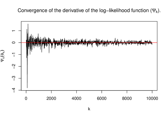
Figure 2: Convergence of the derivative of the log-likelihood function ($\Psi_{k}$). Simulation parameters: $\lambda=1,\>\mu=1,\>\theta=0.02,\>C=1,\>p=15$.

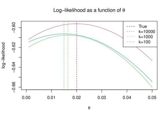
Figure 3: Log-likelihood as a function of $\theta$. Simulation parameters: $\lambda=1,\>\mu=1,\>C=1,\>p=15$,  k=100/1000/10000.

Figures 3 and 4 demonstrate the result of Theorem 1. As $k$ grows, the estimated value of $\theta$ approaches the true value. Figure 3 does not provide information about the goodness of estimation, however, as seen in Figure 4, even for small $k$, the estimated $\theta$ is close enough to the true $\theta$ and converges to it as $k$ grows. As Figure 3 demonstrates, even after 10000 steps the estimated $\theta$ is close to the true one. However, as $k$ grows, it approaches the true value, which demonstrates the consistency of the estimator.

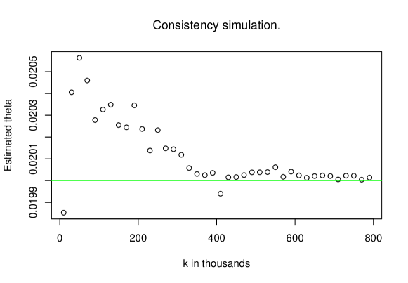
Figure 4: Consistency simulation. Simulation parameters: $\lambda=1,\>\mu=1,\>\theta=0.02,\>C=1,\>p=15$. The plot shows the convergence of the estimated $\theta$ to the true value as $k$ grows.

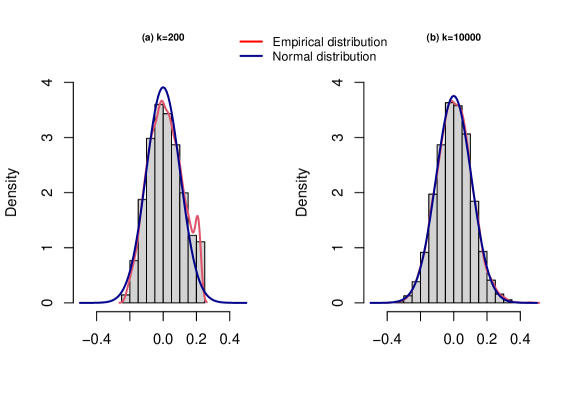
Figure 5: Histogram of normalized estimation errors. Simulation parameters: $\lambda=1,\>\mu=1,\>\theta=0.02,\>C=1,\>p=15$, repeats=5000. The red line stands for estimated density. The blue line stands for normal distribution with a mean of 0 and a standard deviation the same as that of the estimated distribution. For k=200, the mean value is 0.015 and the p-value of the Shapiro-Wilk test is $\sim$ 0 . For k=10000, the mean value is 0.002 and the p-value of the Shapiro-Wilk test is 0.11 .

Figure 5 demonstrates the main result of Theorem 2. When the sample is small, the normalized estimation error distribution is not normal, neither according to Shapiro-Wilk test nor visually. However, for $k=10000$, they are normally distributed around $0$.

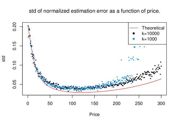
Figure 6: Theoretical and empirical std of normalized estimation error as a function of price. Simulation parameters: $\lambda=1,\>\mu=1,\>C=1,\>\theta=0.02$,   k=1000/10000, repeats for each price.

As was shown in Theorem 2, the variance of asymptotic errors distribution is

$$\left(\mathbb{E}\left[\frac{\mu\lambda(F^{\prime}_{\theta}(Q_{0},\theta))^{2}}{(1-F(Q_{0},\theta))(\mu+\lambda(1-F(Q_{0},\theta)))^{2}}\right]\right)^{-1}.$$

The stationary distribution of $Q_{0}$ can be calculated with (6) and (7). The actual variance can be calculated by simulation of $k$ - steps queue, $n$ - times. Finally, that can be done for different prices. Figure 6 compares the theoretical std and std from such simulation. The probable reason for the difference between the empirical and theoretical std is that the standard deviation of the empirical distribution is an upward-biased, but consistent estimator for standard deviation. As the price grows, the effective sample size is smaller for a fixed number of steps and estimation is more biased. As a result, a higher number of steps lead to better estimation even for high prices.

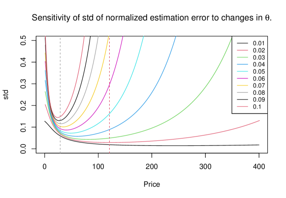
Figure 7: Sensitivity of std of normalized estimation error to changes in $\theta$. Simulation parameters: $\lambda=1,\>\mu=1,\>C=1$. Dashed lines show the prices that minimize std for $\theta=0.02$ (121) and $\theta=0.08$ (29).

Figure 8: Sensitivity of expected revenue to changes in $\theta$. Simulation parameters: $\lambda=1,\>\mu=1,\>C=1$. Dashed lines show the prices that maximize revenue for $\theta=0.02$ (50.9) and $\theta=0.08$ (13).

From Figure 7 one can learn that for any $\theta$ exists a price, that minimizes the standard deviation of the estimation error. This, in turn, provides a better estimation, and correspondingly faster convergence (on average). In addition, the std growth is slower to the right of the optimal price, than to the left. Similar results can be observed in Figure 8, when the price is too low or too high the revenue decreases, however somewhere exists an optimal price. And again, the revenue declines much faster for prices lower than optimal, rather than for prices higher than optimal. This analysis leads to the conclusion that if there are no prior beliefs about the optimal price, the learning should be started from high prices. This strategy will lead to both lower revenue losses per customer and faster convergence. However, as we show further, this analysis does not include important information which affects the choice of the initial price.

Now, we apply the suggested pricing algorithm to the exponential example. Tables 1 and 2 summarize 100 simulations with different initial conditions: minimum observations number ($k_{1}^{min}$), initial price ($p_{1}$), and two different functions used in order to calculate the $k_{i}^{min}$ for every iteration: $k_{i+1}^{min}=g(k_{i})=k_{i}+1$ and $k_{i+1}^{min}=g(k_{i})=2k_{i}$. For example, suppose that $k_{1}^{min}=2$. When 2 observations are gathered the solution is calculated, if the solution is internal, the algorithm will move to the next iteration and $k_{2}^{min}=g(2)$ is calculated. If the solution is on the boundary, additional observation will be gathered and the solution will be calculated again. If the solution is internal, the algorithm will move to the next iteration and $k_{2}^{min}=g(3)$ is calculated. The simulations were constructed in such a way, that the total number of used observations is close as possible.

We compare different combinations of $g(k_{i})$, $p_{1}$ and $k_{i}^{min}$ using number of metrics. In Figures 9, 10 and 11 each point is one iteration, however, the $x$ axis unit is the total number of used observations until the iteration (including). This allows us to compare the learning process of different combinations. The $y$ axis of the figures represents the metric per iteration. For example, in Figure 9, the first point of the combination $(k_{i+1}^{min}=2k_{i},\>p_{1}=15,\>k_{1}=100)$ is located on coordinates $(100,15)$ which is the initialization point. The second point is $(300,52)$ which means that $k_{2}=200$ and $p_{2}=52$. The $y$ axis in Figure 10 is the fraction of maximum revenue, defined as $\frac{\Pi(\hat{p}_{i},\theta)}{\Pi(p,\theta)}$ where $\hat{p}_{i}$ is the price estimated in iteration $i-1$. The $y$ axis in Figure 11 is the total revenue loss at the iteration $i$ which is defined as $t_{i}\left(\Pi(p,\theta)-\Pi(\hat{p}_{i},\hat{\theta_{i}})\right)$.

In the summary tables, the definitions are slightly different. The final stationary fraction of maximum revenue is $\frac{\Pi(\hat{p}_{l},\theta)}{\Pi(p,\theta)}$ where $\hat{p}_{l}$ is the last price estimated before we stopped the learning and $p$ is the optimal price. Stationary cumulative fraction of maximum revenue is $\sum_{i=1}^{l}t_{i}\Pi(\hat{p}_{i},\theta)/\sum_{i=1}^{l}t_{i}\Pi(p,\theta)$. Where $\sum_{i=1}^{l}t_{i}\Pi(p,\theta)$ is the maximum possible revenue of all iterations before the learning stopped, while $\sum_{i=1}^{l}t_{i}\Pi(\hat{p}_{i},\theta)$ is the received revenue during all iterations before the learning stopped. The total lost revenue is defined as $\sum_{i=1}^{l}\left(t_{i}\Pi(p,\theta)-t_{i}\Pi(\hat{p}_{i},\hat{\theta_{i}})\right)$.

$g(k_{i})$	$k_{i}+1$
$k_{1}^{min}$	2				100
$p_{1}$	1	15	100	250	1	15	100	250
Iterations	45.79	47.03	46	37.9	14.86	14.99	15	14.27
Total number of observations used for learning	1531	1530	1532	1529	1591	1604	1605	1552
Final stationary fraction of max revenue	0.988	0.991	0.994	0.995	0.993	0.997	0.998	0.998
Stationary cumulative fraction of max revenue	0.965	0.971	0.973	0.633	0.936	0.967	0.955	0.292
Total lost revenue	1491	1433	1622	27370	2699	1700	2423	128724
Mean error of final price	6.194	5.31	4.42	4.1	4.35	3.072	2.65	2.608
Std of final price error	3.33	3	2.59	2.4	3.18	2.32	2.06	1.87

Table 1: Summary table of 100 simulations for different $p_{1}$, $k_{1}^{min}$ with $g(k_{i})=k_{i}+1$.

For $k_{i+1}^{min}=2k_{i}+1$ function we can see a clear correlation between the price and the distribution of the final price. Both, the mean error of the final price and the std of the error decrease as the initial price grows. However, this correlation is less clear for $k_{i+1}^{min}=2k_{i}$ function. Though, overall, a higher initial price leads to faster convergence. The same is true for a higher $k_{1}^{min}$. Higher $k_{1}^{min}$ clearly correlates with better results for $k_{i+1}^{min}=2k_{i}+1$ function, however not so obvious for $k_{i+1}^{min}=2k_{i}$ function and correct only for high prices. The change of function from $k_{i+1}^{min}=2k_{i}+1$ to $k_{i+1}^{min}=2k_{i}$ will always improve the convergence rate. The result of better convergence can be seen in higher revenue which is closer to the maximum (achieved with the optimal price).

$g(k_{i})$	$2k_{i}$
$k_{1}^{min}$	2				100
$p_{1}$	1	15	100	250	1	15	100	250
Iterations	7.62	8.17	7.96	6.32	4	4	4	4
Total number of observations used for learning	1507	1547	1584	1512	1502	1500	1500	1533
Final stationary fraction of max revenue	0.994	0.994	0.996	0.996	0.983	0.991	0.995	0.996
Stationary cumulative fraction of max revenue	0.978	0.979	0.976	0.636	0.915	0.955	0.95	0.293
Total lost revenue	1164	992	1301	27451	3223	2083	2507	128602
Mean error of final price	2.75	2.89	2.64	2.49	3.89	2.94	2.22	2.51
Std of optimal price error	2.18	2.18	1.99	1.98	3.11	2.34	1.82	1.89

Table 2: Summary table of 100 simulations for different $p_{1}$, $k_{1}^{min}$ with $g(k_{i})=2k_{i}$.

Though, faster learning with a high $p_{1}$ is achieved at the expense of the revenue gained during the learning period. The higher the price, the lower the effective arrival rate, the more time required to gather the desired number of observations, and the higher the revenue loss. As a result, requiring more observations enhance this effect. The too-low price also leads to higher loss, though, the desired sample will be gathered in a short time, thus the total loss will be much smaller (the loss can be much higher if production cost is taken into account). This result disagrees with our previous analysis of revenue as a function of the price which didn’t take the effect of the time required to gather the data into account.

As a general guideline, we can conclude that as we expected, for faster convergence (in sample size terms) it is better to use more observations and high prices. However, if the too high price was chosen by chance, the losses will be very high.

In Figures 9, 10 and 11 there is additional information about the convergence process. In those figures, we present the learning process of the same simulations in more detail with averaged data. First, we can see that whatever $g(k_{i})$ and $p_{1}$ are chosen, if the learning starts $k_{1}^{min}=100$, $p_{2}$ usually will be already close to the optimal. The revenue will also be 90% of the optimal or higher. As was previously predicted, a high initial price leads to higher stationary revenue. However, this effect takes place only at the very beginning of the learning process since the revenue approaches the maximum fast enough for every combination.

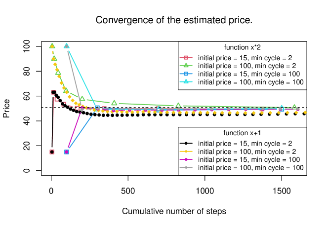
Figure 9: Convergence of the estimated price for different initial prices, minimum observation numbers, and observation number growth functions. Simulation parameters: $\lambda=1,\>\mu=1,\>C=1,\>\theta=0.02$.

The behavior of the loss is more complicated. In some combinations, the loss after the first estimation is higher than that of the initial iteration. It is most easy to see for $(k_{i+1}^{min}=2k_{i},\>p_{1}=15,\>k_{1}=100)$ combination. However, it happens on a lower scale also for other combinations. It occurs in those cases where $p_{2}$ is high. In many cases, the first estimated price ($p_{2}$) is close to 100, even when the $p_{1}$ is 15. As a result, in Figure 9, there is a jump from 15 to 60 (on average over simulations) after the first iteration. This is not surprising, since as we saw in Figure 7, the std of the estimation error is high for low prices. For a larger sample, $k_{1}=100$ this happens more rarely, and on average the $p_{2}$ is very close to the optimal. However, as was previously mentioned, high price also leads to high data aggregation time and hence to higher loss. Therefore, when $k_{2}$ is 200, this effect is very strong even though it (high $p_{2}$) occurs rarely.

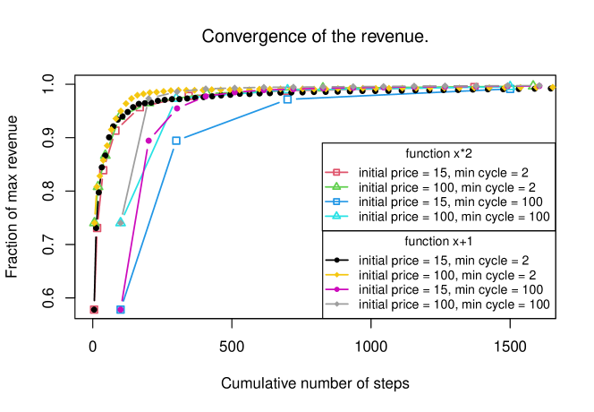
Figure 10: Convergence of the revenue to the maximum revenue for different initial prices, minimum observation numbers, and observation number growth functions. Simulation parameters: $\lambda=1,\>\mu=1,\>C=1,\>\theta=0.02$.

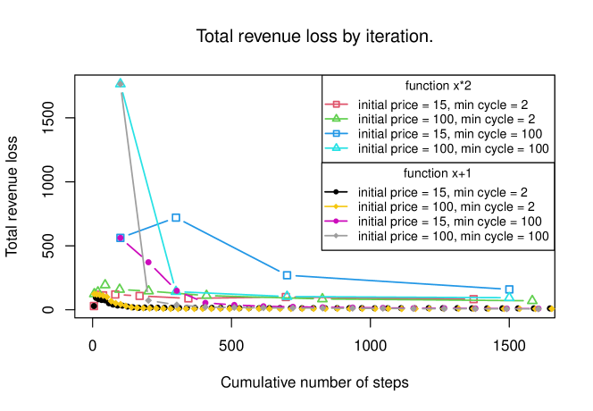
Figure 11: Total revenue loss by iteration for different initial prices, minimum observation numbers, and observation number growth functions. Simulation parameters: $\lambda=1,\>\mu=1,\>C=1,\>\theta=0.02$.

In general, we can see that usually the price and revenue are close to optimal and the losses are very low after 300 - 500 observations in any initialization. However, this result is correct on average, and in specific cases, it is unclear when one can stop the optimization process. As simulations show, the stopping rule we proposed leads to convergence with a small estimation error (with tol=0.01). On average, the number of observations used for learning using this rule is about 1500 - 2000 for $k_{i+1}^{min}=k_{i}+1$ function and $k_{1}^{min}=2$. If $k_{1}^{min}=100$, the numbers grow to 2500 - 3000. With $k_{i+1}^{min}=2k_{i}$ function, the total number of observations can reach 100000 and 200000 with $k_{1}^{min}=2$ and $k_{1}^{min}=100$ correspondingly. However again, with more data, better optimization is achieved.

6 Conclusions and extensions.

In this work, we relaxed the assumption of homogeneous value from completed service ($R$) in Naor’s model. We showed that, under standard assumptions, the maximum likelihood estimator for an unknown parameter of the known distribution of $R$ is consistent, and the normalized errors are asymptotically normal around 0 with a covariance matrix that can be computed. These results were demonstrated using simulation experiments, assuming an exponential distribution for $R$. Additionally, an iterative price maximization algorithm based on the estimator was constructed and applied to simulation data to demonstrate the estimator’s usefulness.

It is straightforward to extend our analysis to more general queues, such as M/M/s or M/M/1/r (which still have an underlying birth-death process). Another possibility is to relax another assumption of Naor’s model—the homogeneity of customers’ patience ($C$). A similar approach can be used to construct an MLE for a common joint distribution of $R$ and $C$. In such a setting, a customer joins the queue if $\frac{R-p}{C}\geq\frac{q_{i}+1}{\mu}$. The distribution of $\frac{R-p}{C}$ can be viewed as one with an additional known parameter $p$. In a special case where $p=0$, our estimator can serve as the MLE for the parameter of the common distribution of $\frac{R}{C}$. For $p>0$, estimating the joint distribution of $R$ and $C$ for a fixed price becomes less straightforward. One possibility is to construct a two-step procedure that first estimates the parameters for different prices, then seeks an optimal solution in the second step.

A similar approach is often found in information technology, where a new service is initially offered for free to attract as many users as possible and study their characteristics. Later, the service becomes paid. The proposed approach assumes that the cost to a customer for staying in the system per unit of time is a linear function of the expected service time $\frac{q_{i}+1}{\mu}$, with service times exponentially distributed. Once these assumptions are removed and the cost to a customer for staying in the system per unit of time is considered as some distribution of expected waiting time, $C(w(q_{i}))$, more general models can be constructed.

The estimator can also be applied to more complex price optimization problems with constraints, such as limitations on price update frequency, production costs, and other economic parameters. The algorithm we presented can also be improved into a more sophisticated, gradient-descent-like or stochastic-descent-like algorithm. In summary, we believe that the approach presented here can lead to multiple interesting research questions to be explored in future work.

Appendix A Proofs

First we introduce a few expressions frequently used throughout the proofs. Recall that the gradient of the log-likelihood is given by

$$\nabla\log\mathcal{L}(\boldsymbol{\theta}|Q_{k},Y_{k}):=\boldsymbol{\Psi}_{k}(\boldsymbol{\theta})=\frac{1}{k}\sum_{i\in M}\boldsymbol{\psi}(Q_{i-1},Y_{i},\boldsymbol{\theta})$$

where, for any $q\geq 0$ and $y\in\{0,1\}$,

$$\boldsymbol{\psi}(q,y,\boldsymbol{\theta})=\begin{bmatrix}y\frac{p^{\prime}_{\theta_{1}}(q,\boldsymbol{\theta})}{p(q,\boldsymbol{\theta})}-(1-y)\frac{p^{\prime}_{\theta_{1}}(q,\boldsymbol{\theta})}{1-p(q,\boldsymbol{\theta})}\\ \\ \vdots\\ \\ y\frac{p^{\prime}_{\theta_{n}}(q,\boldsymbol{\theta})}{p(q,\boldsymbol{\theta})}-(1-y)\frac{p^{\prime}_{\theta_{n}}(q,\boldsymbol{\theta})}{1-p(q,\boldsymbol{\theta})}\end{bmatrix}$$ (11)

The upward transition probability (given $\boldsymbol{\theta}$) from state $q$ is

$$p(q,\boldsymbol{\theta})=\frac{\lambda(1-F(r(q)),\boldsymbol{\theta})))}{\mu+\lambda(1-F(r(q),\boldsymbol{\theta}))},$$ (12)

where $r(q)=p+\frac{(q+1)C}{\mu}$. For any $j=1,\ldots,n$, taking derivative with respect to $\theta_{j}$ yields

$$p^{\prime}_{\theta_{j}}(q,\boldsymbol{\theta}):=\frac{\partial p(q,\boldsymbol{\theta})}{\partial\theta_{j}}=-\frac{\mu\lambda F^{\prime}_{\theta_{j}}(r(q),\boldsymbol{\theta})}{(\mu+\lambda(1-F(r(q),\boldsymbol{\theta})^{2}},$$ (13)

and once more with respect to $\theta_{l}$, for any $l=1,\ldots,n$,

$$p^{\prime\prime}_{\theta_{j}\theta_{l}}(q,\boldsymbol{\theta})=\frac{-\mu\lambda[F^{\prime\prime}_{\theta_{j}\theta_{l}}(r(q),\boldsymbol{\theta})(\mu+\lambda(1-F(r(q),\boldsymbol{\theta})+2\lambda F^{\prime}_{\theta_{j}}(r(q),\boldsymbol{\theta})F^{\prime}_{\theta_{l}}(r(q),\boldsymbol{\theta})]}{(\mu+\lambda(1-F(r(q),\boldsymbol{\theta})^{3}},$$ (14)

where $p^{\prime\prime}_{\theta_{j}\theta_{l}}(q,\boldsymbol{\theta}):=\frac{\partial p^{\prime}_{\theta_{j}}(q,\boldsymbol{\theta})}{\partial\theta_{l}}$.

By Assumption A2, all of the expressions above are well defined for any $(q,y)$ such that $F(r(q),\boldsymbol{\theta})\in(0,1)$, and the first derivative $p^{\prime}_{\theta_{j}}(q,\boldsymbol{\theta})$ is continuous w.r.t. $\boldsymbol{\theta}$ for every $j=1,\ldots,n$. Note that for our results the second derivative need not be continuous, i.e., $F^{\prime\prime}$ exists but may have discontinuities.

A.1 Consistency (proofs of Lemmas 1-5)

Lemma 1.

If $F(r(q),\boldsymbol{\theta})$ is continuous, twice differentiable and has a continuous first derivative, w.r.t. $\boldsymbol{\theta}\in\boldsymbol{\Theta}$ (Assumption A2), then $\boldsymbol{\psi}_{i}(q,y,\boldsymbol{\theta})$ is continuous w.r.t. $\boldsymbol{\theta}\in\boldsymbol{\Theta}$, for any $(q,y)$ such that $F(r(q),\boldsymbol{\theta})\in(0,1)$.

Proof.

Observe that the denominator of (13) is strictly positive for any $q$ such that $F(r(q),\boldsymbol{\theta})\in(0,1)$. Therefore, as $F$ and its first derivative is continuous with respect to $\boldsymbol{\theta}\in\boldsymbol{\Theta}$, we conclude from (11) and (12) that $\boldsymbol{\psi}$ is also a continuous function.

∎

Lemma 2.

Suppose Assumption A3 holds, then

$$\max_{j=1\ldots,n}\left|\boldsymbol{\Psi}_{k}(\boldsymbol{\boldsymbol{\theta}})\right|_{j}\leq 2H(q)\ ,\forall q:F(r(q),\boldsymbol{\theta})\in(0,1),$$

where $H$ is the integrable function in Assumption A3.

Proof.

For any $j=1,\ldots,n$,

$$\psi^{j}(q,y,\boldsymbol{\theta})=y\frac{p^{\prime}_{\theta_{j}}(q,\boldsymbol{\theta})}{p(q,\boldsymbol{\theta})}+(1-y)\frac{p^{\prime}_{\theta_{j}}(q,\boldsymbol{\theta})}{1-p(q,\boldsymbol{\theta})},$$

hence, as $y\in\{0,1\}$, the triangle inequality yields

$$\left|\psi^{j}(q,y,\boldsymbol{\theta})\right|\leq\left|\frac{p^{\prime}_{\theta_{j}}(q,\boldsymbol{\theta})}{p(q,\boldsymbol{\theta})}\right|+\left|\frac{p^{\prime}_{\theta_{j}}(q,\boldsymbol{\theta})}{1-p(q,\boldsymbol{\theta})}\right|,$$ (15)

By (12) and (13),

$$\left|\frac{p^{\prime}_{\theta_{j}}(q,\boldsymbol{\theta})}{1-p(q,\boldsymbol{\theta})}\right|=\left|-\frac{\lambda F^{\prime}_{\theta_{j}}(r(q),\boldsymbol{\theta})}{\mu+\lambda(1-F(r(q),\boldsymbol{\theta}))}\right|<\left|\frac{F^{\prime}_{\theta_{j}}(r(q),\boldsymbol{\theta}))}{1-F(r(q),\boldsymbol{\theta})}\right|,$$ (16)

and

$$\frac{p^{\prime}_{\theta_{j}}(q,\boldsymbol{\theta})}{p(q,\boldsymbol{\theta})}=-\frac{\mu F_{\theta_{j}}^{\prime}(r(q),\boldsymbol{\theta})}{(1-F(r(q),\boldsymbol{\theta}))(\mu+\lambda(1-F(r(q),\boldsymbol{\theta})))}=\frac{-F_{\theta_{j}}^{\prime}(r(q),\boldsymbol{\theta})}{1-F(r(q),\boldsymbol{\theta})}\cdot\frac{\mu}{\mu+\lambda(1-F(r(q),\boldsymbol{\theta}))}.$$

Note that $0\leq F(r(q),\boldsymbol{\theta})\leq 1$. As a result

$$\frac{\mu}{\mu+\lambda}\leq\frac{\mu}{\mu+\lambda(1-F(r(q),\boldsymbol{\theta}))}\leq 1,$$

thus,

$$\left|\frac{p^{\prime}_{\theta_{j}}(q,\boldsymbol{\theta})}{p(q,\boldsymbol{\theta})}\right|=\left|\frac{-F_{\theta_{j}}^{\prime}(r(q,\boldsymbol{\theta})}{1-F(r(q),\boldsymbol{\theta})}\cdot\frac{\mu}{\mu+\lambda(1-F(r(q),\boldsymbol{\theta}))}\right|\leq\left|\frac{F^{\prime}_{\theta_{j}}(r(q),\boldsymbol{\theta}))}{1-F(r(q),\boldsymbol{\theta})}\right|.$$ (17)

Combining the above with (15) and Assumption A3 we conclude that

$$\max_{j=1,\ldots,n}\left|{\psi}^{j}(q,y,\boldsymbol{\theta})\right|_{j}\leq 2\max_{j=1,\ldots,n}\left|\frac{\nabla_{\boldsymbol{\theta}}F(r(q),\boldsymbol{\theta})}{1-F(r(q),\boldsymbol{\theta})}\right|\leq 2H(q).$$

The proof is completed by recalling that $\boldsymbol{\Psi}_{k}(\boldsymbol{\boldsymbol{\theta}})=\frac{1}{k}\sum_{i=1}^{k}\boldsymbol{\psi}(Q_{i-1},Y_{i},\boldsymbol{\theta})$.

∎

Lemma 3.

A unique stationary distribution $(Q_{0},Y_{1})$ exists and for any function $g:\mathbb{N}\times\{0,1\}\to\mathbb{R}$ such that $\mathbb{E}[|g(Q_{0},Y_{1})|]<\infty$,

$$\frac{1}{k}\sum_{i\in M}g(Q_{i-1},Y_{i})\overset{a.s.}{\longrightarrow}\mathbb{E}[g(Q_{0},Y_{1})]\>\>\text{as}\>\>k\rightarrow\infty.$$

Further, if Assumption A3  holds, then for any $\boldsymbol{\theta}\in\boldsymbol{\Theta}$,

$$\boldsymbol{\Psi}_{k}(\boldsymbol{\theta})\overset{a.s.}{\longrightarrow}\boldsymbol{\Psi}(\boldsymbol{\theta})\>\>\text{as }\>k\rightarrow\infty.$$

Proof.

An irreducible birth-death process with rates $(\lambda_{0},\mu_{1},\lambda_{1},\mu_{2},\lambda_{2},...,)$ is ergodic and has a unique stationary distribution if the following conditions hold (see [14]):

$$\sum_{k=1}^{\infty}\prod_{q=1}^{k}\frac{\lambda_{q-1}}{\mu_{q}}<\infty,$$ (18)

$$\sum_{k=1}^{\infty}\prod_{q=1}^{k}\frac{\mu_{q}}{\lambda_{q}}=\infty.$$ (19)

Recall that $r(q)=p+\frac{C(q+1)}{\mu}$. Also, $\mu_{q}=\mu$ for all $q$. In addition, $F(r,\boldsymbol{\theta})$ is a CDF, therefore $\lim_{r\rightarrow\infty}{F(r,\boldsymbol{\theta})}=1$, consequently

$$\lim_{q\rightarrow\infty}\lambda_{i}=\lim_{q\rightarrow\infty}\lambda\left(1-F\left(p+\frac{C(q+1)}{\mu}\right)\right)=0.$$ (20)

We first verify (18). From (20) it follows that $\lambda_{q}\rightarrow 0$ as $q\rightarrow\infty$. Thus there exists a $q$ such that $\frac{\lambda_{q-1}}{\mu}<1$. Let

$$q_{0}=\underset{q}{\text{arg min}}\left\{q:\frac{\lambda_{q-1}}{\mu}<1\right\},$$

then we can rewrite

$$\sum_{k=1}^{\infty}\prod_{q=1}^{k}\frac{\lambda_{q-1}}{\mu}=\omega_{0}+\sum_{k=q_{0}}^{\infty}\prod_{q=1}^{k}\frac{\lambda_{q-1}}{\mu},$$ (21)

where $\omega_{0}:=\sum_{k=1}^{q_{0}-1}\prod_{q=1}^{k}\frac{\lambda_{q-1}}{\mu}$ is a positive finite number. Similarly,

$$\prod_{q=1}^{k}\frac{\lambda_{q-1}}{\mu}=\omega_{1}\prod_{q=q_{0}}^{k}\frac{\lambda_{q-1}}{\mu},$$ (22)

where $\omega_{1}\>=\prod_{q=1}^{q_{0}-1}\frac{\lambda_{q-1}}{\mu}$ is a finite positive number larger than $1$. Combining (21) and (22) yields

$$\sum_{k=1}^{\infty}\prod_{q=1}^{k}\frac{\lambda_{q-1}}{\mu}=\omega_{0}+\omega_{1}\sum_{k=q_{0}}^{\infty}\prod_{q=q_{0}}^{k}\frac{\lambda_{q-1}}{\mu}.$$ (23)

Now, since $F(r,\boldsymbol{\theta})$ is monotone increasing function, we have that for any $q$, $\frac{\lambda_{q}}{\mu}<\frac{\lambda_{q-1}}{\mu}$, and in particular

$$\frac{\lambda_{q_{0}+1}}{\mu}<\frac{\lambda_{q_{0}}}{\mu}.$$

As a result, for any $k\geq q_{0}+1$

$$\prod_{q=q_{0}}^{k}\frac{\lambda_{q-1}}{\mu}<\left(\frac{\lambda_{q_{0}}}{\mu}\right)^{k-q_{0}+1}.$$

Combining this with (23), we have that

$$\omega_{0}+\omega_{1}\sum_{k=q_{0}}^{\infty}\prod_{q=q_{0}}^{k}\frac{\lambda_{q-1}}{\mu}<\omega_{0}+\omega_{1}\sum_{k=q_{0}}^{\infty}\left(\frac{\lambda_{q_{0}}}{\mu}\right)^{k-q_{0}+1}.$$

Since $\frac{\lambda_{q_{0}}}{\mu}<1$, it follows that $\sum_{k=q_{0}}^{\infty}\left(\frac{\lambda_{q_{0}}}{\mu}\right)^{k-q_{0}+1}<\infty$. Thus, (18) is verified.

We next verify (19). As was shown previously, $\lambda_{q}\rightarrow 0$ as $q\rightarrow\infty$ while $\mu$ is constant. Thus $\frac{\mu_{q}}{\lambda_{q}}=\frac{\mu}{\lambda_{q}}\rightarrow\infty$ when $q\rightarrow\infty$, hence

$$\sum_{k=1}^{\infty}\prod_{i=1}^{k}\frac{\mu}{\lambda_{q}}=\infty$$

as required. We conclude that $(Q_{i},y)_{i\geq 0}$ is an ergodic sequence and a unique stationary distribution $Q_{0},Y_{1}$ exists. Moreover, by Ergodic Theorem in [8, Ch. 6], for any ergodic sequence, and, for any integrable function $g$ there exists a limit

$$\frac{1}{k}\sum_{i\in M}g(Q_{i-1},Y_{i})\overset{a.s.}{\longrightarrow}\mathbb{E}[g(Q_{0},Y_{1})]<\infty.$$

Further, if Assumption A3  holds, then Lemma 2 implies that $\boldsymbol{\Psi}_{k}(\boldsymbol{\theta})\overset{a.s.}{\longrightarrow}\boldsymbol{\Psi}(\boldsymbol{\theta})$ for any $\boldsymbol{\theta}\in\boldsymbol{\Theta}$. ∎

Lemma 4.

If Assumptions A3 holds, then for any $\epsilon>0$.

$$\inf_{\boldsymbol{\theta}:d(\boldsymbol{\theta},\boldsymbol{\theta}_{0})\geq\epsilon}||\boldsymbol{\Psi}(\boldsymbol{\theta})||>0=||\boldsymbol{\Psi}(\boldsymbol{\theta}_{0})||.$$

Proof.

Applying Lemma 3 together with (16), for any $\boldsymbol{\theta}$ there exists a limit as $k\to\infty$,

$$\frac{1}{k}\sum_{i\in M}\left[Y_{i}\frac{p^{\prime}_{\theta_{j}}(Q_{i-1},\boldsymbol{\theta})}{p(Q_{i-1},\boldsymbol{\theta})}\right]\overset{a.s.}{\longrightarrow}\mathbb{E}\left[Y_{1}\frac{p^{\prime}_{\theta_{j}}(Q_{0},\boldsymbol{\theta})}{p(Q_{0},\boldsymbol{\theta})}\right]<\infty.$$

Now, using the law of total expectation

$$\mathbb{E}\left[Y_{1}\frac{p^{\prime}_{\theta_{j}}(Q_{0},\boldsymbol{\theta})}{p(Q_{0},\boldsymbol{\theta})}\right]=\mathbb{E}\left[\mathbb{E}\left[Y_{1}\frac{p^{\prime}_{\theta_{j}}(Q_{0},\boldsymbol{\theta})}{p(Q_{0},\boldsymbol{\theta})}|Q_{0}\right]\right].$$

Observe that given $Q_{0}$ the distribution of $Y_{1}$ is Bernoulli with probability $p(Q_{0},\boldsymbol{\theta}_{0})$, therefore

$$\mathbb{E}\left[\mathbb{E}\left[Y_{1}\frac{p^{\prime}_{\theta_{j}}(Q_{0},\boldsymbol{\theta})}{p(Q_{0},\boldsymbol{\theta})}\right]|Q_{0}\right]=\mathbb{E}\left[\frac{p^{\prime}_{\theta_{j}}(Q_{0},\boldsymbol{\theta})}{p(Q_{0},\boldsymbol{\theta})}\mathbb{E}\left[Y_{1}|Q_{0}\right]\right]=\mathbb{E}\left[\frac{p^{\prime}_{\theta_{j}}(Q_{0},\boldsymbol{\theta})}{p(Q_{0},\boldsymbol{\theta})}p(Q_{0},\boldsymbol{\theta}_{0})\right].$$

Only for $\boldsymbol{\theta}=\boldsymbol{\theta}_{0}$ we obtain

$$\mathbb{E}\left[\mathbb{E}\left[Y_{1}\frac{p^{\prime}_{\theta_{j}}(Q_{0},\boldsymbol{\theta}_{0})}{p(Q_{0},\boldsymbol{\theta}_{0})}\right]|Q_{0}\right]=\mathbb{E}\left[p^{\prime}_{\theta_{j}}(Q_{0},\boldsymbol{\theta}_{0})\right]$$ (24)

We will use similar arguments for the second part of the estimating equation. Specifically, by Lemma 3 and (17),

$$\frac{1}{k}\sum_{i\in M}\left[(1-y)\frac{p^{\prime}_{\theta_{j}}(Q_{i-1},\boldsymbol{\theta})}{1-p(Q_{i-1},\boldsymbol{\theta})}\right]\overset{a.s.}{\longrightarrow}\mathbb{E}\left[(1-Y_{1})\frac{p^{\prime}_{\theta_{j}}(Q_{0},\boldsymbol{\theta})}{1-p(Q_{0},\boldsymbol{\theta})}\right]<\infty.$$

Applying the law of total expectation yields,

$$\mathbb{E}\left[(1-Y_{1})\frac{p^{\prime}_{\theta_{j}}(Q_{0},\boldsymbol{\theta})}{1-p(Q_{0},\boldsymbol{\theta})}\right] =\mathbb{E}\left[\mathbb{E}\left[(1-Y_{1})\frac{p^{\prime}_{\theta_{j}}(Q_{0},\boldsymbol{\theta})}{1-p(Q_{0},\boldsymbol{\theta})}|Q_{0}\right]\right]=\mathbb{E}\left[\frac{p^{\prime}_{\theta_{j}}(Q_{0},\boldsymbol{\theta})}{1-p(Q_{0},\boldsymbol{\theta})}\mathbb{E}\left[1-Y_{1}|Q_{0}\right]\right]$$

$$=\mathbb{E}\left[\frac{p^{\prime}_{\theta_{j}}(Q_{0},\boldsymbol{\theta})}{1-p(Q_{0},\boldsymbol{\theta})}(1-p(Q_{0}|\boldsymbol{\theta}_{0}))\right].$$

Plugging in $\boldsymbol{\theta}=\boldsymbol{\theta}_{0}$ yields

$$\mathbb{E}\left[(1-Y_{1})\frac{p^{\prime}_{\theta_{j}}(Q_{0},\boldsymbol{\theta}_{0})}{1-p(Q_{0},\boldsymbol{\theta}_{0})}\right]=\mathbb{E}\left[p^{\prime}_{\theta_{j}}(Q_{0},\boldsymbol{\theta}_{0})\right].$$ (25)

Then combination of (24), (25) and (11) completes the proof of Lemma 4. ∎

Lemma 5.

If Assumptions A1, A2, A3 hold, then

$$\boldsymbol{\Psi}_{k}(\hat{\boldsymbol{\theta}}_{k})\overset{a.s.}{\longrightarrow}\boldsymbol{0}\>$$

and consequently

$$\boldsymbol{\Psi}_{k}(\hat{\boldsymbol{\theta}}_{k})\overset{P}{\longrightarrow}\boldsymbol{0}\>.$$

Proof.

Lemmas 1-3 imply that $\boldsymbol{\Psi}_{k}(\hat{\boldsymbol{\theta}})$ converges uniformly on the compact set $\boldsymbol{\Theta}$ to the function $\boldsymbol{\Psi}(\hat{\boldsymbol{\theta}})$ on $\boldsymbol{\Theta}$ (see [9, Thm. 16a]). By Lemma 4 and Assumption A1, $\boldsymbol{\Psi}(\boldsymbol{\theta})$) has a unique root $\boldsymbol{\theta}_{0}\in\boldsymbol{\Theta}^{\mathrm{o}}$ (the interior of the compact parameter space). Therefore, there exists a constant $\delta>0$ such that

$$\inf_{\boldsymbol{\theta}\notin\boldsymbol{\Theta}^{\mathrm{o}}}|\boldsymbol{\Psi}(\hat{\boldsymbol{\theta}})|_{j}\geq\delta,\forall j=1,\ldots,n.$$

Moreover, as $\boldsymbol{\Theta}^{\mathrm{o}}\subset\boldsymbol{\Theta}$ (2), implies that

$$\inf_{\boldsymbol{\theta}\notin\boldsymbol{\Theta}^{\mathrm{o}}}\min_{j=1,\ldots,n}|\boldsymbol{\Psi}_{k}(\hat{\boldsymbol{\theta}})|\overset{\mathrm{a.s.}}{\longrightarrow}\delta>0.$$

Thus, with probability one, there exists an integer $N$, such that all coordinates of $\inf_{\boldsymbol{\theta}\notin\boldsymbol{\Theta}^{\mathrm{o}}}\boldsymbol{\Psi}(\hat{\boldsymbol{\theta}})$ are non-zero for any $k>N$. I.e., the MLE is given by an interior solution for any $k>N$. We conclude that $\boldsymbol{\Psi}_{k}(\hat{\boldsymbol{\theta}}_{k})\overset{a.s.}{\longrightarrow}0$ which also implies $\boldsymbol{\Psi}_{k}(\hat{\boldsymbol{\theta}}_{k})\overset{p}{\longrightarrow}0$ and completes the proof. ∎

A.2 Filtration of the queue-length random walk.

Previously we defined the random process $Q_{i}$ in a natural and intuitive way. Here we define $Q_{i}$ in a formal way. The rigorous definition is useful for some proofs and enables a deeper understanding from a probabilistic angle. Firstly we define the probability space $(\Omega_{k},\mathcal{F}_{i},\mathrm{P}_{i})$ for $Q_{i}$. Let $\Omega_{k}$ be the sample space of a queue process after $k$ steps. $\Omega_{k}$ includes all possible paths which are sets of length $k+1$ of the form $\{0,q_{1},q_{2},...,q_{k}\}$. Such that $q_{1}=1$ and $q_{i}\in\{q_{i-1}-1,q_{i-1}+1\}$ for ${2\leq i\leq k}$.

Let $\mathcal{F}_{i}$ be a $\sigma$-algebra of step $i$. Define

$$\phi_{m}^{i-1}=\left\{\bigcup_{j\in\Gamma_{m}}\omega_{j}\right\},$$

where

$$\Gamma_{m}=\left\{j:w_{j}\in\{0,q_{1},q_{2},...,q_{i-1},\cdot\}_{m}\right\},$$

where $0,q_{1},q_{2},...,q_{i-1}$ is a specific path $m$ and “$\cdot$” is some unknown path. Also, $m\in M_{i-1}$ where $M_{i-1}$ is a group of all possible paths $0,q_{1},q_{2},...,q_{i-1}$.

Then $\mathcal{F}_{i}$ is a set of all $m\in M_{i-1}$ sets $\phi_{m}^{i-1}$ and their unions in every possible combination, and $\emptyset$.

Also, every $\phi_{m}^{i}$ is $\left\{\bigcup_{j\in\Gamma_{m}}\omega_{j}\right\}$, $m\in M_{i}$ where $M_{i}$ is a group of all possible paths $0,q_{1},q_{2},...,q_{i}$. Then for each $m\in M_{i}$, $\phi_{m}^{i}$ is the union of $w$ of the form $\{0,q_{1},q_{2},...,q_{i-1},q_{i-1}+1,\cdot\}$ or $\{0,q_{1},q_{2},...,q_{i-1},q_{i-1}-1,\cdot\}$. $\mathcal{F}_{i}$ include all sets $\phi_{m}^{i}$ as well as their unions in every possible combination and a $\emptyset$.

However, for every $m\in M_{i-1}$, $\phi_{m}^{i-1}$ is a union of $\phi_{m}^{i}$ of the form $\{0,q_{1},q_{2},...,q_{i-1},q_{i-1}+1,\cdot\}$ with $\phi_{m}^{i}$ of the form $\{0,q_{1},q_{2},...,q_{i-1},q_{i-1}-1,\cdot\}$. Then every $\phi_{m}^{i-1}\in\mathcal{F}_{i}$, as well as any union of $\phi_{m}^{i-1}$, where $m\in M_{i-1}$ is a subset of $\mathcal{F}_{i}$. As a result, $\mathcal{F}_{i-1}\subseteq\mathcal{F}_{i}$, which allows us to conclude that $\{\mathcal{F}_{i}\}_{i\geq 0}$ is filtration.

Now we define a sequence of random variables $(Q_{i})_{0\leq i\leq k}:(\Omega_{k},\mathcal{F}_{i},\mathrm{P}_{i})\rightarrow(\mathbb{Z}^{+},\{0,1,...,i\},F_{i})$ as $i$-th element of $\omega$, i.e. $Q_{i}(\omega)=q_{i}$. The sequence of random variables $Q_{i}$ is adapted to the filtration $\mathcal{F}_{i}$.

The experiment is designed in such a way that the queue length increases if a new customer joins earlier than the currently served person leaves (since the service is finished) and decreases if the opposite occurs. Thus the queue length naturally satisfies the Markov property. It follows that $(Q_{i})_{0\leq i\leq k}$ is discrete-time Markov chain with transition matrix

$$\Pi_{j,q}=\left\{\begin{matrix}\left\{\begin{matrix}1&,\>\>q>j\\ 0&,\>\>q<j\end{matrix}\right.&,\>\>j=0\\ \left\{\begin{matrix}\frac{\lambda_{j}}{\mu+\lambda_{j}}&,\>\>q>j\\ \frac{\mu}{\mu+\lambda_{j}}&,\>\>q<j\end{matrix}\right.&,\>\>j>0\end{matrix}\right.$$

Assuming that $q_{0}=0$ the probability mass function of $Q_{i}$ is $(\Pi^{i})_{0}$ where index $0$ is the first row of the matrix $(\Pi^{i})$. The probability $\mathrm{P}(Q_{i}=q)=(\Pi^{i})_{0,q}$ and cumulative distribution function is

$$F_{i}(q)=\sum_{j=0}^{q}(\Pi^{i})_{0,j}$$

The probability of $\phi_{m}^{i-1}$ is the probability to see a path $q_{i},q_{i-1},q_{i-2},...,q_{0}$, which, using the Markov property, is :

$$\mathrm{P}(\phi_{m}^{i-1})=\mathrm{P}(Q_{i}=q_{i},Q_{i-1}=q_{i-1},Q_{i-2}=q_{i-2},...,Q_{0}=q_{0})=\prod_{i=1}^{k}P(Q_{i}=q_{i}|Q_{i-1}=q_{i-1})=\prod_{i=1}^{k}\Pi_{i-1,i}\>.$$

Each group in $\mathcal{F}_{i}$ is a union of $\phi_{m}^{i-1}$, i.e. $\cup_{m\in L}\left\{\phi_{m}^{i-1}\right\}$ where $L$ is some set of $m\in M_{i-1}$. Thus:

$$\mathrm{P}(\cup_{m\in L}\left\{\phi_{m}^{i-1}\right\})=\sum_{m\in L}\mathrm{P}(\phi_{m}^{i-1})\>.$$

Finally, $\boldsymbol{\psi}_{i}(Q_{i-1},Y_{i},\boldsymbol{\theta})$ as defined in (11) is almost everywhere continuous, hence it is measurable and the sequence $(\boldsymbol{\psi}_{i}(Q_{i-1},Y_{i},\boldsymbol{\theta}))_{i\geq 1}$ is adapted to the filtration $\mathcal{F}_{i}$.

A.3 Proof of Lemma 6

Lemma 6.

If Assumptions A1-A4 hold, then

$$\boldsymbol{\nabla}\boldsymbol{\Psi}_{k}^{-1}(\boldsymbol{\theta_{0}})\overset{\mathrm{a.s.}}{\longrightarrow}\boldsymbol{\nabla}\boldsymbol{\Psi}^{-1}(\boldsymbol{\theta_{0}})\ ,$$

where

$$-\boldsymbol{\nabla}\boldsymbol{\Psi}(\boldsymbol{\theta}_{0})=\mathbb{E}[\boldsymbol{\psi}(Q_{0},Y_{1},\boldsymbol{\theta}_{0})\boldsymbol{\psi}(Q_{0},Y_{1},\boldsymbol{\theta}_{0})^{T}]=\boldsymbol{\Sigma}.$$

Proof.

Recall that $\boldsymbol{\Psi}_{k}(\boldsymbol{\theta})=\frac{1}{k}\sum_{i=1}^{k}\boldsymbol{\psi}(Q_{i-1},Y_{i},\boldsymbol{\theta})$. We will first compute the ergodic limit of the Jacobian at $\boldsymbol{\theta}_{0}$ (assuming, for now, that it exists),

$$(\nabla\boldsymbol{\Psi}_{k}(\boldsymbol{\theta}_{0}))_{jl}=\left(\frac{1}{k}\sum_{i=1}^{k}\frac{\partial}{\partial\theta_{l}}{\psi}^{j}(Q_{i-1},Y_{i},\boldsymbol{\theta})\right)_{jl}.$$

By (11),

$$\frac{\partial}{\partial\theta_{l}}{\psi}^{j}(q,y,,\boldsymbol{\theta})=\frac{\partial}{\partial\theta_{l}}\left(y\frac{p^{\prime}_{\theta_{j}}(q,\boldsymbol{\theta})}{p(q,\boldsymbol{\theta})}\right)-\frac{\partial}{\partial\theta_{l}}\left((1-y)\frac{p^{\prime}_{\theta_{j}}(q,\boldsymbol{\theta})}{1-p(q,\boldsymbol{\theta})}\right).$$

$$\frac{\partial}{\partial\theta_{l}}\left(y\frac{p^{\prime}_{\theta_{j}}(q,\boldsymbol{\theta})}{p(q,\boldsymbol{\theta})}\right)=y\frac{p^{\prime\prime}_{\theta_{j}\theta_{l}}(q,\boldsymbol{\theta})p(q,\boldsymbol{\theta})-p^{\prime}_{\theta_{l}}(q,\boldsymbol{\theta})p^{\prime}_{\theta_{j}}(q,\boldsymbol{\theta})}{(p(q,\boldsymbol{\theta}))^{2}},$$

where the second derivative is well defined due to Assumption A2. For $\boldsymbol{\theta}=\boldsymbol{\theta}_{0}$, the stationary mean, i.e., with respect to the distribution of $(Q_{0},Y_{1})$, is computed using the law of total expectation,

$$\mathbb{E}\left[Y_{1}\frac{p^{\prime\prime}_{\theta_{j}\theta_{l}}(Q_{0},\boldsymbol{\theta}_{0})p(Q_{0},\boldsymbol{\theta}_{0})-p^{\prime}_{\theta_{l}}(Q_{0},\boldsymbol{\theta}_{0})p^{\prime}_{\theta_{j}}(Q_{0},\boldsymbol{\theta}_{0})}{(p(Q_{0},\boldsymbol{\theta}_{0}))^{2}}\right]=\mathbb{E}\left[\frac{p^{\prime\prime}_{\theta_{j}\theta_{l}}(Q_{0},\boldsymbol{\theta}_{0})p(Q_{0},\boldsymbol{\theta}_{0})-p^{\prime}_{\theta_{l}}(Q_{0},\boldsymbol{\theta}_{0})p^{\prime}_{\theta_{j}}(Q_{0},\boldsymbol{\theta}_{0})}{p(Q_{0},\boldsymbol{\theta}_{0})}\right].$$

Similarly, the derivative of the second part is

$$\frac{\partial}{\partial\theta_{l}}\left((1-y)\frac{p^{\prime}_{\theta_{j}}(q,\boldsymbol{\theta})}{1-p(q,\boldsymbol{\theta})}\right)=(1-y)\frac{p^{\prime\prime}_{\theta_{j}\theta_{l}}(q,\boldsymbol{\theta})(1-p(q,\boldsymbol{\theta}))+p^{\prime}_{\theta_{l}}(q,\boldsymbol{\theta})p^{\prime}_{\theta_{j}}(q,\boldsymbol{\theta})}{(1-p(q,\boldsymbol{\theta}))^{2}},$$

Again, for $\boldsymbol{\theta}=\boldsymbol{\theta}_{0}$, the stationary mean, i.e., with respect to the distribution of $(Q_{0},Y_{1})$, the law of total expectation again yields

$$\mathbb{E}\left[(1-Y_{1})\frac{p^{\prime\prime}_{\theta_{j}\theta_{l}}(Q_{0},\boldsymbol{\theta}_{0})(1-p(Q_{0},\boldsymbol{\theta}_{0}))+p^{\prime}_{\theta_{l}}(Q_{0},\boldsymbol{\theta}_{0})p^{\prime}_{\theta_{j}}(Q_{0},\boldsymbol{\theta}_{0})}{(1-p(Q_{0},\boldsymbol{\theta}_{0}))^{2}}\right]$$

$$=\mathbb{E}\left[\frac{p^{\prime\prime}_{\theta_{j}\theta_{l}}(Q_{0},\boldsymbol{\theta}_{0})(1-p(Q_{0},\boldsymbol{\theta}_{0}))+p^{\prime}_{\theta_{l}}(Q_{0},\boldsymbol{\theta}_{0})p^{\prime}_{\theta_{j}}(Q_{0},\boldsymbol{\theta}_{0})}{1-p(Q_{0},\boldsymbol{\theta}_{0})}\right]$$

Observe that at $\theta=\theta_{0}$, for every $j,l$,

$$\mathbb{E}\left[\frac{p^{\prime\prime}_{\theta_{j}\theta_{l}}(Q_{0},\boldsymbol{\theta}_{0})(1-p(Q_{0},\boldsymbol{\theta}_{0}))}{1-p(Q_{0},\boldsymbol{\theta}_{0})}\right]=\mathbb{E}\left[\frac{p^{\prime\prime}_{\theta_{j}\theta_{l}}(Q_{0},\boldsymbol{\theta}_{0})p(Q_{0},\boldsymbol{\theta}_{0})}{p(Q_{0},\boldsymbol{\theta}_{0})}\right]=\mathbb{E}\left[p^{\prime\prime}_{\theta_{j}\theta_{l}}(Q_{0},\boldsymbol{\theta}_{0})\right].$$

As expectation is linear, combining the derivatives of the two parts yields

$$\mathbb{E}\left[\frac{\partial}{\partial\theta_{l}}{\psi}^{j}(Q_{0},Y_{1},\boldsymbol{\theta}_{0})\right]=\mathbb{E}\left[\frac{-p^{\prime}_{\theta_{l}}(Q_{0},\boldsymbol{\theta}_{0})p^{\prime}_{\theta_{j}}(Q_{0},\boldsymbol{\theta}_{0})}{(1-p(Q_{0},\boldsymbol{\theta}_{0}))p(Q_{0},\boldsymbol{\theta}_{0})}\right].$$

For any $j,l$, plugging in the expressions in (12) and (13) yields

$$\mathbb{E}\left[\frac{\partial}{\partial\theta_{l}}{\psi}^{j}(Q_{0},Y_{1},\boldsymbol{\theta}_{0})\right]=-\mathbb{E}\left[\frac{\lambda\mu F^{\prime}_{\theta_{j}}(r(Q_{0}),\boldsymbol{\theta}_{0})F^{\prime}_{\theta_{l}}(r(Q_{0}),\boldsymbol{\theta}_{0})}{(1-F(r(Q_{0}),\boldsymbol{\theta}_{0}))(\mu+\lambda(1-F(r(Q_{0}),\boldsymbol{\theta}_{0})))^{2}}\right]=-\Sigma_{jl}.$$

By Assumption A4 we have that $|\Sigma_{jl}|<\infty$, thus Lemma 3 implies that for any $j,l\in\{1,\ldots,n\}$

$$(\nabla\boldsymbol{\Psi}_{k}(\boldsymbol{\theta}_{0}))_{jl}=\left(\frac{1}{k}\sum_{i=1}^{k}\frac{\partial}{\partial\theta_{l}}{\psi}^{j}(Q_{i-1},Y_{i},\boldsymbol{\theta})\right)_{jl}\overset{\mathrm{a.s.}}{\longrightarrow}-\Sigma_{jl},$$

where $|\Sigma_{jl}|<\infty$ for all $j,l$.

The last remaining step is computing the stationary variance of the martingale sequence. As $\mathbb{E}\left[{\psi}^{j}(Q_{0},Y_{1},\boldsymbol{\theta}_{0})\right]=0$ for all $j=1,\ldots,n$, the variance of the martingale difference is the matrix

$$\mathbb{E}\left[\boldsymbol{\psi}(Q_{0},Y_{1},\boldsymbol{\theta}_{0})\boldsymbol{\psi}(Q_{0},Y_{1},\boldsymbol{\theta}_{0})^{T}\right].$$

The entry at coordinate $j,l$ is given by

$$\mathbb{E}\left[Y_{1}^{2}\frac{p^{\prime}_{\theta_{j}}(Q_{0},\boldsymbol{\theta})p^{\prime}_{\theta_{l}}(Q_{0},\boldsymbol{\theta})}{p^{2}(Q_{0},\boldsymbol{\theta})}-2Y_{1}(1-Y_{1})\frac{p^{\prime}_{\theta_{j}}(Q_{0},\boldsymbol{\theta})p^{\prime}_{\theta_{l}}(Q_{0},\boldsymbol{\theta})}{p(Q_{0},\boldsymbol{\theta})(1-p(Q_{0},\boldsymbol{\theta}))}+(1-Y_{1})^{2}\frac{p^{\prime}_{\theta_{j}}(Q_{0},\boldsymbol{\theta})p^{\prime}_{\theta_{l}}(Q_{0},\boldsymbol{\theta})}{(1-p(Q_{0},\boldsymbol{\theta}))^{2}}\right],$$

and as $Y_{1}(1-Y_{1})=0$, applying the law of total expectation once more yields

$$\left(\mathbb{E}\left[\boldsymbol{\psi}(Q_{0},Y_{1},\boldsymbol{\theta}_{0})\boldsymbol{\psi}(Q_{0},Y_{1},\boldsymbol{\theta}_{0})^{T}\right]\right)_{jl} =\mathbb{E}\left[\frac{p^{\prime}_{\theta_{j}}(Q_{0},\boldsymbol{\theta}_{0})p^{\prime}_{\theta_{l}}(Q_{0},\boldsymbol{\theta}_{0})}{p(Q_{0},\boldsymbol{\theta}_{0})}+\frac{p^{\prime}_{\theta_{j}}(Q_{0},\boldsymbol{\theta}_{0})p^{\prime}_{\theta_{l}}(Q_{0},\boldsymbol{\theta}_{0})}{(1-p(Q_{0},\boldsymbol{\theta}_{0}))}\right]$$

$$=\mathbb{E}\left[\frac{p^{\prime}_{\theta_{j}}(Q_{0},\boldsymbol{\theta}_{0})p^{\prime}_{\theta_{l}}(Q_{0},\boldsymbol{\theta}_{0})}{p(Q_{0},\boldsymbol{\theta}_{0})(1-p(Q_{0},\boldsymbol{\theta}_{0}))}\right]=\Sigma_{jl}.$$

∎

References

• [1] P. Aféche a d B. Ata (2013). Bayesian Dynamic Pricing in Queueing Systems with Unknown Delay Cost Characteristics. Manufacturing & Service Operations Management 15 (2):292–304.
• [2] Z. Akşin, B. Ata, S.M. Emadi, C.L. Su (2013). Structural estimation of callers’ delay sensitivity in call centers. Management Science, 59:2727–2746.
• [3] A Asanjarani, Y Nazarathy, and P Taylor (2021). A survey of parameter and state estimation in queues. Queueing Systems, 97:39–80.
• [4] P. Billingsley (1961). Statistical methods in Markov chains. The Annals of Mathematical Statistics, 32(10):12–40.
• [5] S.A. Bodas, M. Mandjes and L. Ravner (2023). Statistical inference for a service system with non-stationary arrivals and unobserved balking. arXiv preprint arXiv:2311.16884.
• [6] V.I. Bogachev, (2007). Measure Theory. Springer Science & Business Media.
• [7] X. Chen, Y. Liu and G. Hong (2023). An online learning approach to dynamic pricing and capacity sizing in service systems. Operations Research.
• [8] R. Durret, (2019). Probability: Theory and Examples. Cambridge University Press.
• [9] T. Ferguson (1996). A Course in Large Sample Theory. Chapman & Hall, Routledge.
• [10] R. Hassin (2016). Rational Queueing, CRC Press.
• [11] R. Hassin, M. Haviv(2003). To Queue or Not to Queue: Equilibrium Behavior in Queueing Systems, Springer.
• [12] M. Haviv (2013). Queues - A Course in Queueing Theory, volume 191 of International Series in Operations Research & Management Science. Springer.
• [13] Y Inoue, L Ravner, and M Mandjes (2023). Estimating customer impatience in a service system with unobserved balking. Stochastic Systems, 13(2):181–210.
• [14] S. Karlin and J. McGregor (1957). The Classification of Birth and Death Processes.. Transactions of the American Mathematical Society, 86 (2): 366–400.
• [15] C. Larsen (1998). Investigating sensitivity and the impact of information on pricing decisions in an M/M/$1/\infty$ queueing model. International Journal of Production Economics, , 56,:365–377.
• [16] P. Naor (1969). The regulation of queue size by levying tolls. Econometrica, 37:15–24.
• [17] L. Ravner and R.I. Snitkovsky (2023). Stochastic approximation of symmetric nash equilibria in queueing games. Operations Research.
• [18] L. Ravner and J. Wang (2023). Estimating customer delay and tardiness sensitivity from periodic queue length observations. Queueing Systems, 103(3):241–274.
• [19] A. van der Vaart (1998). Asymptotic Statistics, volume 3. Cambridge University Press.
• [20] A. van der Vaart (2010). Time series. VU Amsterdam, lecture notes.
• [21] W. Whitt (2012). Fitting birth-and-death queueing models to data. Statistics & Probability Letters, 82(5):998–1004.