Maximal work extraction unitarily from an unknown quantum state:
Ergotropy estimation via feedback experiments
Abstract
Considering the emerging applications of quantum technologies, studying energy storage and usage at the quantum level is of great interest. In this context, there is a significant contemporary interest in studying ergotropy, the maximum amount of work that can be extracted unitarily from an energy-storing quantum device. Here, we propose and experimentally demonstrate a feedback-based algorithm (FQErgo) for estimating ergotropy. This method also transforms an arbitrary initial state to its passive state, which allows no further unitary work extraction. FQErgo applies drive fields whose strengths are iteratively adjusted via certain expectation values, conveniently read using a single probe qubit. Thus, FQErgo provides a practical way for unitary energy extraction and for preparing passive states. By numerically analyzing FQErgo on random initial states, we confirm the successful preparation of passive states and estimation of ergotropy, even in the presence of drive errors. Finally, we implement FQErgo on two- and three-qubit NMR registers, prepare their passive states, and accurately estimate their ergotropy.
I Introduction
Quantum technologies are appealing as they can surpass their classical counterparts by using exclusive concepts like coherence and entanglement. Understanding their capabilities has progressed in recent years, thanks to the numerous experimental breakthroughs that have improved control over quantum states. Specifically, the investigation of the principles of quantum thermodynamics is made possible by quantum thermal machines, which include refrigerators and heat engines to regulate heat flow and work production [1, 2]. Further options for storing energy for later extraction include quantum batteries [3, 4, 5, 6, 7, 8, 9, 10, 11, 12, 13, 14]. In every possible framework, like charging speed [15, 16, 17, 18, 19, 20], stored energy [21, 22], and energy extraction [23, 24, 25, 26, 27], the quantum batteries have the potential to outperform their classical counterparts.
The maximum amount of energy that can be extracted from quantum systems through unitary processes is known as the ergotropy [28]. A practical way to determine ergotropy is by finding the optimal unitary operation that transforms the system to its lowest attainable energy state, known as its passive state [29]. This can be a challenging undertaking as ergotropy might be sensitive to correlations that can also impact device performance [30, 31, 32, 33, 34, 35, 36, 37]. Recent works have tried to establish a link between entanglement and thermodynamic quantities like the ergotropy gap, the difference between the maximal extractable works via global and local unitaries. These thermodynamic quantities can be used to verify entanglement present in bipartite [38], multipartite [39, 40], and multiqubit mixed states [41]. Using these quantities, experimental certification of entanglement has been demonstrated in up to 10 qubits [41].
The main focus of this work is FQErgo, an algorithm we propose for preparing the passive state and thereby estimating ergotropy. FQErgo is inspired by (hence the name) the feedback-based algorithm for quantum optimization (FALQON) [42], which has been recently developed for combinatorial quantum optimization. This method uses feedback conditioned on qubit measurements at each quantum circuit layer and parametrized quantum circuits to determine the values of the circuit parameters at subsequent layers. FALQON is related to quantum Lyapunov control (QLC), a feedback procedure to find the controls needed to manipulate a quantum system’s dynamics in a desired way [43, 44].
We note several salient features of the FQErgo algorithm. Firstly, the all-quantum nature of the algorithm: unlike the previous methods [45, 46] for estimating ergotropy, FQErgo requires no classical optimizer. Secondly, FQErgo is robust against circuit errors since each feedback iteration readjusts the drives based on previous errors. This way, cumulative error growth is prevented. Thirdly, the circuit parameters can be read efficiently via an ancillary probe qubit using the interferometric method [47, 48, 49]. This way alleviates the need for resource-intensive quantum state tomography. Lastly, being a feedback-based method, FQErgo can be fully automated for convenient practical realizations. In this work, after numerically analyzing the FQErgo algorithm, we experimentally demonstrate it using two and three-qubit NMR registers.
This article is organized as follows. In Sec. II, we describe the theoretical construction of FQErgo algorithm. In Sec. III, we numerically analyze FQErgo over random sets of initial states in one and two-qubit systems. The NMR implementations of FQErgo for both one and two-qubit systems with an additional probe qubit are reported in Sec. IV. Finally, Sec. V summarizes the results and discusses their importance.
II Theory
II.1 Unitary extraction of work, passive state, and ergotropy
Given a quantum system in a state , the ergotropy quantifies the maximum amount of work that is unitarily extracted while leaving the system into a passive state from which no further work can be unitarily extracted [28]. If is the system Hamiltonian, the ergotropy is given by
| (1) |
Let corresponds to the unitary that minimizes the system energy such that is the passive state [28, 29]. If and , in their respective eigenbases, are in the form
| (2) |
then the passive state is uniquely defined in the energy eigenbasis as
| (3) |
While the above definitions of the passive state and ergotropy are simple and clear, the experimental realization of the passive state from an unknown initial state and thereby estimating its ergotropy has not been reported. In the following, we describe a robust method for the same.
II.2 FQErgo: A feedback algorithm for ergotropy estimation
FQErgo is based on the FALQON algorithm proposed recently [42]. We assume multiple copies of individually accessible systems each prepared in the state , which is not necessarily known. Alternatively, we assume a quantum system that can be repeatedly prepared into the same unknown state . On introducing a drive Hamiltonian , the system evolves as
| (4) |
where is the time-dependent drive parameter. Here and in the rest of the paper we have set . We seek to minimize the system energy , which can be accomplished by designing control such that
| (5) |
where . One way to satisfy the above is by choosing the control in the form [42]
| (6) |
where is a positive scalar coefficient.
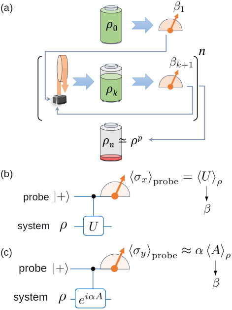
The overall algorithm is illustrated in Fig. 1 (a). We apply discrete drives each of duration and realize a -step feedback loop,
| (7) |
We find the first drive parameter by measuring the expectation value , and prepare the state . The subsequent steps involve finding
| (8) |
Thus, starting from an unknown quantum state , using the sequence of feedback-designed operators , we attain the minimum saturated energy state . The energy measurements of the system for the initial state and the final state yield an estimation of ergotropy via Eq. 1.
II.3 FQErgo using a probe qubit
FQErgo described above needs an efficient method to repeatedly extract expectation values of the commutator in Eq. 6, and to monitor the system-energy. Since quantum state tomography is prohibitively expensive for such a task, we shall use the interferometric circuit with an ancillary probe qubit [47, 45, 46]. The interferometric circuit for measuring the energy as well as extracting the drive parameter in Eq. 8 are shown in Fig. 1 (b,c). The circuit involves preparing the probe qubit in the state, the system in any state , applying a certain controlled operation on the system, and finally measuring the probe qubit. First, consider extracting the expectation value of a unitary Hermitian observable . In this case, we implement a controlled gate as shown in Fig. 1 (b). The probe signal is then given by,
| (9) |
Thus, we directly obtain the desired expectation value of the system as the signal in the probe qubit. For example, if the system Hamiltonian is the Pauli operator as described later in the experimental section, the probe signal directly yields the expectation value . For the more general case of extracting the expectation value of a nonunitary Hermitian observable , we construct a unitary , where is a scalar parameter such that . Now implementing the controlled gate as shown in Fig. 1 (c), we obtain the probe signal
| (10) |
Here, by setting , we can extract directly as the probe signal .
III Numerical simulations
III.1 Single qubit system
We consider a single qubit system with Hamiltonian with energy eigenvalues prepared in an arbitrary mixed state , where and the purity parameter . We now use FQErgo to reach its passive state . For the one qubit case, FQErgo needs only two drives: and . Fig. 2 (a) shows the energy versus iteration number for a set of 20 random initial states. In all cases, we see monotonically decreasing energy, ultimately approaching their respective passive states for sufficiently large iterations , i.e., . The difference between the initial energy and the final energy estimates the ergotropy, i.e., . The filled circles in Fig. 2 (c), plotting vs confirm perfect estimation of ergotropy for all the random initial states.
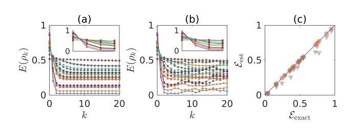
Now we shall analyze the robustness of FQErgo against potential imperfections in practical implementations. Firstly, being a feedback-based method, FQErgo is very robust against the amplitude of the drives. The smaller the drive amplitude, it simply takes longer to reach the passive state. To study the robustness against more general errors, we introduce now an error rotation of 5 degrees about a random direction in every FQErgo iteration. The system-energy curves shown in Fig. 2 (b) do not show perfect monotonic decay, but neither exhibit serious build-up of errors. The corresponding ergotropy values shown by filled triangles in Fig. 2 (c) show somewhat underestimated values, which is expected since circuit errors can make the system settle in only a higher energy state by preventing it from reaching the passive state.
III.2 Two qubit system
For two or more qubits, energy can be extracted using local unitaries on individual systems or global unitaries on the whole system. If we minimize the system energy using only local unitaries, we can get to the local passive state , which determines the local ergotropy . If we minimize the system energy using global unitaries, along with or without local unitaries, we can get to the global passive state , which determines the global ergotropy . The difference is called the ergotropy gap [50].
Consider a two-qubit system with Hamiltonian with and prepared in random initial states . The ergotropy gap is now
| (11) |
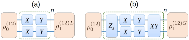
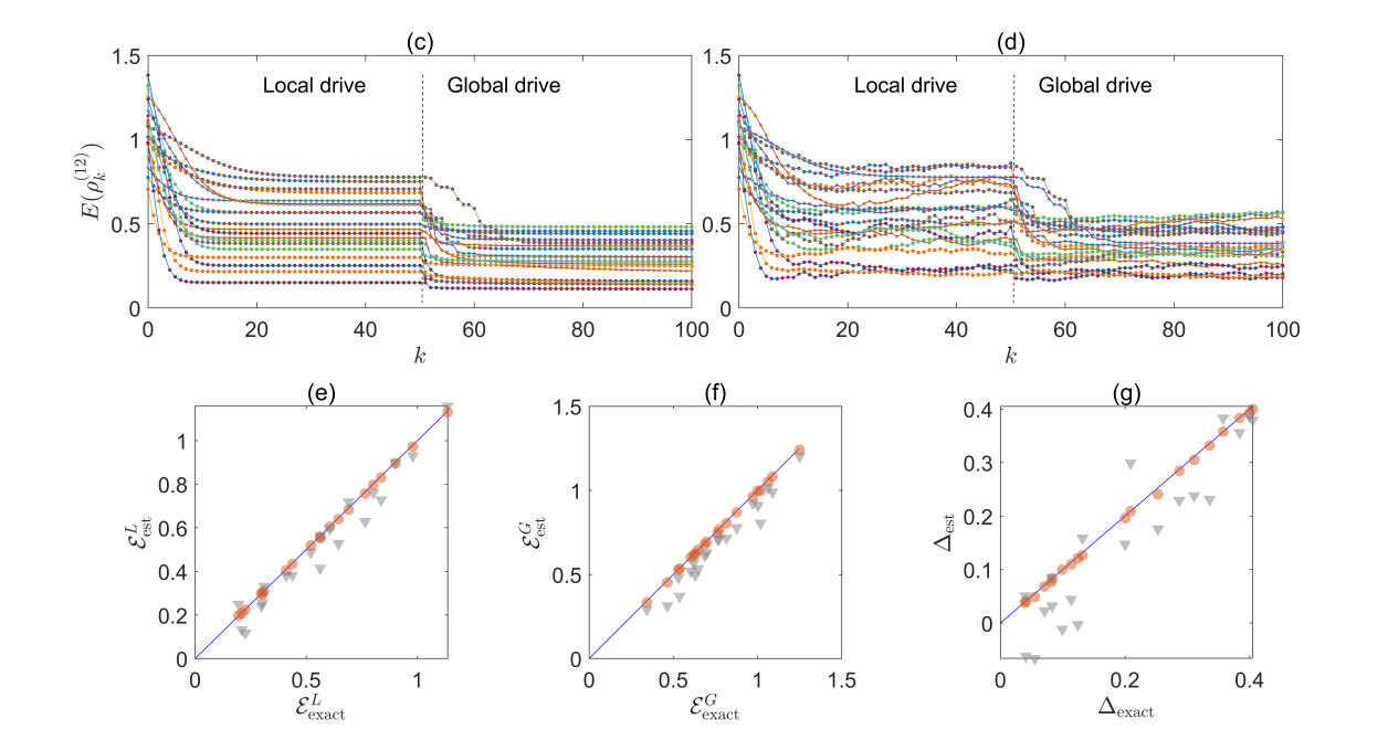
Our goal is to use FQErgo for estimating both local and global ergotropies and thereby obtaining the ergotropy gap. As illustrated in Fig. 3 (a), we use four local drives and , where over the first 30 iterations that saturated the energy and reached , the local passive state. From the 31st iteration, we see a further reduction in energy as we apply a combination of global and local operations, as illustrated in Fig. 3 (b). It involves a tilted phase gate
with a fixed small angle [45], local gates, as well as the global gate,
strength , and duration . Finally, we find the second energy saturation over 60 iterations while reaching , the global passive state. Fig. 3 (c) shows the monotonic energy decrease for 20 random initial states undergoing FQErgo iteration. For each initial state, we observe two minimum-energy states, one corresponding to the local passive state and the other to the global passive state. Figs. 3 (e-f) plot the estimated local and global ergotropies against their exact values, and Fig. 3 (g) plots the estimated ergotropy gaps against exact values.
We now study FQErgo robustness by introducing a random nonlocal error unitary generated by a random unit-norm error Hamiltonian and degrees in every FQErgo iteration. The system-energy curves shown in Fig. 3 (d) lose monotonicity in decay, but retain the overall trend. The error-affected local and global ergotropy values and the corresponding ergotropy gaps are shown by filled triangles in Fig. 3 (e-g). Likewise in one qubit case, the ergotropy values, particularly the global ergotropy values are underestimated, but the rms deviation of the ergotropy gap estimations from the ideal values remains below 0.07 indicating reasonable robustness of FQErgo against local/nonlocal errors.
IV Experiments
IV.1 Single-qubit ergotropy
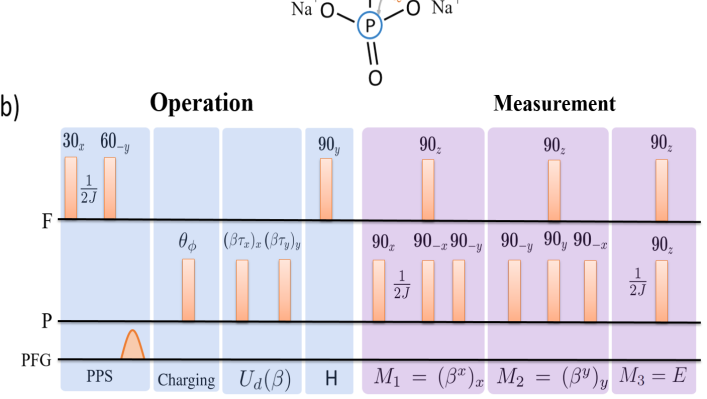
We now use sodium fluorophosphate (dissolved in D2O; Fig. 4(a)) as the two-qubit register, wherein 19F is our probe qubit and 31P is the system qubit. All the experiments were carried out on a MHz Bruker NMR spectrometer at an ambient temperature of K. The rotating frame Hamiltonian of the system consisting of the internal part and the RF drive is , where and , where are the spin operators. Here , and (, ) respectively denote the adjustable frequency offsets and time-dependent RF amplitudes of 19F and 31P spins, and Hz is the scalar coupling constant.
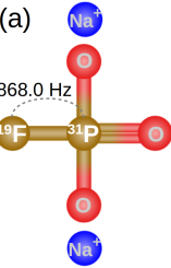
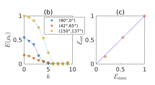
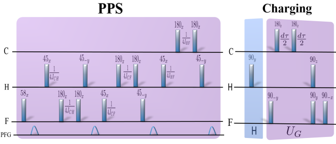
The pulse sequences for the NMR implementations of FQErgo are described in Appendix. Starting from the thermal state, we prepare a pseudopure state (PPS) before energizing the system qubit 31P into one of the three initial states as described in Fig. 4. For FQErgo, we choose the drives and , and their strengths in the th iteration are given by . Notice that all three different states reach their common passive state within 10 iterations in Fig. 4 (b). The corresponding ergotropy values show excellent agreement with the numerically simulated values in Fig. 4 (c), thus demonstrating the successful implementation of FQErgo.
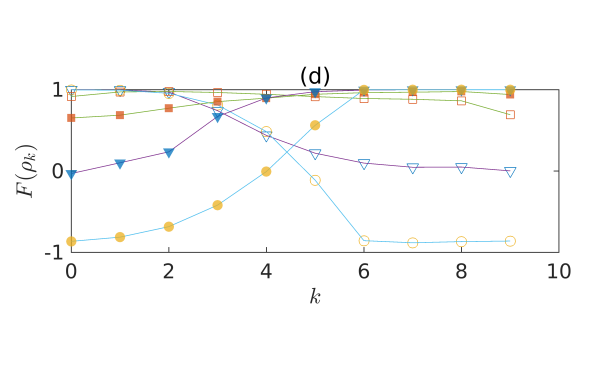
In this one qubit case, since we have now measured all three expectation values , we can now reconstruct the density matrix and determine its state fidelities with the respective initial state and with the expected target passive state, at each iteration. The resulting fidelity profiles are shown in Fig. Fig. 4 (d). They indicate the gradual decay of the initial state fidelity and the corresponding buildup of the passive state fidelity. We clearly find high-fidelity passive states being prepared in each of the three cases.
IV.2 Two-qubit ergotropy
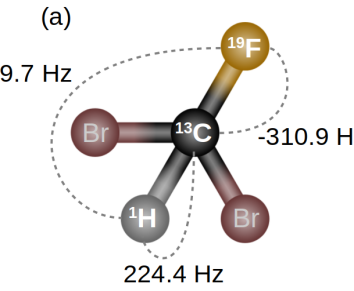
To estimate two-qubit ergotropy, we use the three-spin NMR register dibromofluoromethane (dissolved in Acetone-D6; Fig. 5 (a)). We consider 13C as the probe and 1H, 19F as the system qubits. The rotating frame Hamiltonian consisting of the internal part and the RF drive reads as , where and . Here , and , respectively denote the frequency offsets and RF amplitudes, while denote the scalar coupling constants, whose values are shown in Fig. 5 (a).
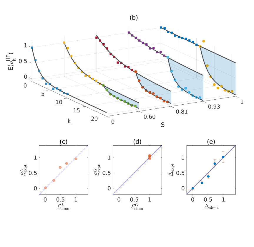
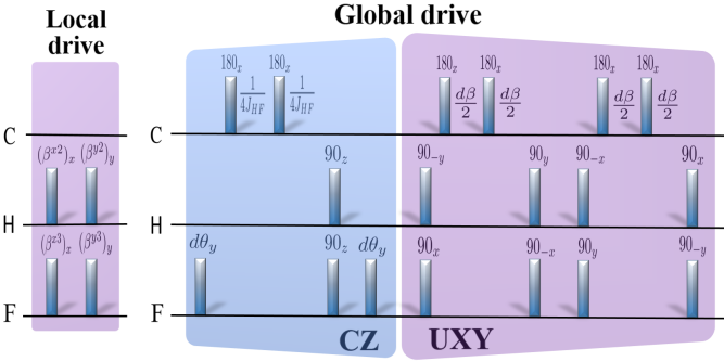
To demonstrate local and global ergotropy estimation, we prepare five initial states with varying degrees of entanglement between the system qubits and . The full NMR pulse-sequences are described in the Appendix. After preparing we transform it to using a global unitary consisting of a Hadamard operator on and a controlled gate on . Note that the parameter controls the degree of entanglement. That completes the initialization, and now we start work extraction by FQErgo. During the first 10 iterations, we extract work by using only local drives , (similar as in Fig. 3 (a)) and realize the first energy minimization corresponding to the local passive state as shown in Fig. 5 (c). From 11th to 20th iterations, we extract further energy via the global drive along with the gate and local drives as shown in Fig. 3 (b). The global drive allows complete work extraction, eventually taking the system qubits to the second energy minimization corresponding to the global passive state . Fig. 5 (b) shows the normalized energies for both local and global extraction with initial states having varying entanglement entropy , where . Fig. 5 (c-d) plot the experimentally estimated local and global ergotropy values vs simulated values and Fig. 5 (e) plots the experimentally obtained ergotropy gaps vs versus the simulated values. The good agreement between the estimated values and the simulated values confirms the successful demonstration of the FQErgo algorithm.
V Summary and discussions
In summary, we have introduced a feedback-based algorithm, FQErgo to prepare the passive state and thereby quantify the ergotropy, the maximum unitarily extractable energy, of an unknown quantum state of a given system. It is an iterative feedback algorithm that efficiently reads certain expectation values using a probe qubit and readjusts the subsequent drive strengths to extract further energy. The same probe qubit also allows regular monitoring of system energy throughout the process. By numerically implementing FQErgo over a set of random states in both one and two-qubit systems, we have verified robust passive state preparation and ergotropy estimation, even in the presence of circuit errors. We then experimentally implemented FQErgo on multiple initial states of two and three-qubit NMR registers, successfully prepared their passive states, and closely estimated their local and global ergotropies as well as the ergotropy gap.
We envisage several future directions. For instance, previously using ergotropy as an entanglement witness required prior knowledge of the class of states (eg. [41]). FQErgo can overcome such limitations and pave the way to certify the entanglement for a completely unknown state. Since one probe-qubit suffices, irrespective of the system size, extending FQErgo to larger systems should be feasible without exponential complexity. Although the ensemble nature of NMR is advantageous here, the overall algorithm is general enough to adapt to other quantum architectures.
Acknowledgements
Authors acknowledges valuable discussions with Pranav Chandarana, Mir Alimuddin, Vishal Varma, Arijit Chatterjee, Harikrishnan, and Conan Alexander. J.J. acknowledges support from CSIR (Council of Scientific and Industrial Research) Project No. 09/936(0259)/2019 EMR - I. We also thank the National Mission on In- terdisciplinary Cyber-Physical Systems for funding from the DST, Government of India, through the I-HUB Quantum Technology Foundation, IISER-Pune and funding from DST/ICPS/QuST/ 2019/Q67.
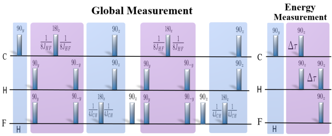
Appendix: NMR pulse sequences
(a)
(b)
(c)
References
- Kosloff and Levy [2014] Ronnie Kosloff and Amikam Levy. Quantum heat engines and refrigerators: Continuous devices. Annual review of physical chemistry, 65(1):365–393, 2014.
- Mitchison [2019] Mark T Mitchison. Quantum thermal absorption machines: refrigerators, engines and clocks. Contemporary Physics, 60(2):164–187, 2019.
- Alicki and Fannes [2013] Robert Alicki and Mark Fannes. Entanglement boost for extractable work from ensembles of quantum batteries. Physical Review E—Statistical, Nonlinear, and Soft Matter Physics, 87(4):042123, 2013.
- Hovhannisyan et al. [2013] Karen V Hovhannisyan, Martí Perarnau-Llobet, Marcus Huber, and Antonio Acín. Entanglement generation is not necessary for optimal work extraction. Physical review letters, 111(24):240401, 2013.
- Rossini et al. [2019] Davide Rossini, Gian Marcello Andolina, and Marco Polini. Many-body localized quantum batteries. Physical Review B, 100(11):115142, 2019.
- Andolina et al. [2019a] Gian Marcello Andolina, Maximilian Keck, Andrea Mari, Michele Campisi, Vittorio Giovannetti, and Marco Polini. Extractable work, the role of correlations, and asymptotic freedom in quantum batteries. Physical review letters, 122(4):047702, 2019a.
- Rodriguez et al. [2024] RR Rodriguez, Borhan Ahmadi, Gerardo Suárez, Paweł Mazurek, S Barzanjeh, and Paweł Horodecki. Optimal quantum control of charging quantum batteries. New Journal of Physics, 26(4):043004, 2024.
- Joshi and Mahesh [2022] Jitendra Joshi and T. S. Mahesh. Experimental investigation of a quantum battery using star-topology nmr spin systems. Phys. Rev. A, 106:042601, Oct 2022. doi: 10.1103/PhysRevA.106.042601. URL https://link.aps.org/doi/10.1103/PhysRevA.106.042601.
- Hu et al. [2022] Chang-Kang Hu, Jiawei Qiu, Paulo JP Souza, Jiahao Yuan, Yuxuan Zhou, Libo Zhang, Ji Chu, Xianchuang Pan, Ling Hu, Jian Li, et al. Optimal charging of a superconducting quantum battery. Quantum Science and Technology, 7(4):045018, 2022.
- Konar et al. [2022] Tanoy Kanti Konar, Leela Ganesh Chandra Lakkaraju, Srijon Ghosh, and Aditi Sen. Quantum battery with ultracold atoms: Bosons versus fermions. Physical Review A, 106(2):022618, 2022.
- Barra et al. [2022] Felipe Barra, Karen V Hovhannisyan, and Alberto Imparato. Quantum batteries at the verge of a phase transition. New Journal of Physics, 24(1):015003, 2022.
- Campaioli et al. [2024] Francesco Campaioli, Stefano Gherardini, James Q Quach, Marco Polini, and Gian Marcello Andolina. Colloquium: quantum batteries. Reviews of Modern Physics, 96(3):031001, 2024.
- Campaioli et al. [2018] Francesco Campaioli, Felix A Pollock, and Sai Vinjanampathy. Quantum batteries. Thermodynamics in the Quantum Regime: Fundamental Aspects and New Directions, pages 207–225, 2018.
- Binder et al. [2015] Felix C Binder, Sai Vinjanampathy, Kavan Modi, and John Goold. Quantacell: powerful charging of quantum batteries. New Journal of Physics, 17(7):075015, 2015.
- Andolina et al. [2019b] Gian Marcello Andolina, Maximilian Keck, Andrea Mari, Vittorio Giovannetti, and Marco Polini. Quantum versus classical many-body batteries. Physical Review B, 99(20):205437, 2019b.
- Ghosh et al. [2020] Srijon Ghosh, Titas Chanda, and Aditi Sen. Enhancement in the performance of a quantum battery by ordered and disordered interactions. Physical Review A, 101(3):032115, 2020.
- Gao et al. [2022] Lei Gao, Chen Cheng, Wen-Bin He, Rubem Mondaini, Xi-Wen Guan, and Hai-Qing Lin. Scaling of energy and power in a large quantum battery-charger model. Physical Review Research, 4(4):043150, 2022.
- Gyhm et al. [2022] Ju-Yeon Gyhm, Dominik Šafránek, and Dario Rosa. Quantum charging advantage cannot be extensive without global operations. Physical Review Letters, 128(14):140501, 2022.
- Salvia et al. [2023] Raffaele Salvia, Martí Perarnau-Llobet, Géraldine Haack, Nicolas Brunner, and Stefan Nimmrichter. Quantum advantage in charging cavity and spin batteries by repeated interactions. Physical Review Research, 5(1):013155, 2023.
- Rodriguez et al. [2023] Ricard Ravell Rodriguez, Borhan Ahmadi, Pawel Mazurek, Shabir Barzanjeh, Robert Alicki, and Pawel Horodecki. Catalysis in charging quantum batteries. Physical Review A, 107(4):042419, 2023.
- Zhang et al. [2019] Yu-Yu Zhang, Tian-Ran Yang, Libin Fu, and Xiaoguang Wang. Powerful harmonic charging in a quantum battery. Physical Review E, 99(5):052106, 2019.
- Andolina et al. [2018] Gian Marcello Andolina, Donato Farina, Andrea Mari, Vittorio Pellegrini, Vittorio Giovannetti, and Marco Polini. Charger-mediated energy transfer in exactly solvable models for quantum batteries. Physical Review B, 98(20):205423, 2018.
- Ferraro et al. [2018] Dario Ferraro, Michele Campisi, Gian Marcello Andolina, Vittorio Pellegrini, and Marco Polini. High-power collective charging of a solid-state quantum battery. Physical review letters, 120(11):117702, 2018.
- Le et al. [2018] Thao P Le, Jesper Levinsen, Kavan Modi, Meera M Parish, and Felix A Pollock. Spin-chain model of a many-body quantum battery. Physical Review A, 97(2):022106, 2018.
- Tirone et al. [2023] Salvatore Tirone, Raffaele Salvia, Stefano Chessa, and Vittorio Giovannetti. Work extraction processes from noisy quantum batteries: The role of nonlocal resources. Physical Review Letters, 131(6):060402, 2023.
- Liu et al. [2021] Jia-Xuan Liu, Hai-Long Shi, Yun-Hao Shi, Xiao-Hui Wang, and Wen-Li Yang. Entanglement and work extraction in the central-spin quantum battery. Physical Review B, 104(24):245418, 2021.
- Monsel et al. [2020] Juliette Monsel, Marco Fellous-Asiani, Benjamin Huard, and Alexia Auffèves. The energetic cost of work extraction. Physical review letters, 124(13):130601, 2020.
- Allahverdyan et al. [2004] Armen E Allahverdyan, Roger Balian, and Th M Nieuwenhuizen. Maximal work extraction from finite quantum systems. EPL (Europhysics Letters), 67(4):565, 2004.
- Pusz and Woronowicz [1978] Wiesław Pusz and Stanisław L Woronowicz. Passive states and kms states for general quantum systems. Communications in Mathematical Physics, 58(3):273–290, 1978.
- Goold et al. [2016] John Goold, Marcus Huber, Arnau Riera, Lídia Del Rio, and Paul Skrzypczyk. The role of quantum information in thermodynamics—a topical review. Journal of Physics A: Mathematical and Theoretical, 49(14):143001, 2016.
- Bera et al. [2017] Manabendra N Bera, Arnau Riera, Maciej Lewenstein, and Andreas Winter. Generalized laws of thermodynamics in the presence of correlations. Nature communications, 8(1):2180, 2017.
- Manzano et al. [2018] Gonzalo Manzano, Francesco Plastina, and Roberta Zambrini. Optimal work extraction and thermodynamics of quantum measurements and correlations. Physical Review Letters, 121(12):120602, 2018.
- Vitagliano et al. [2018] Giuseppe Vitagliano, Claude Klöckl, Marcus Huber, and Nicolai Friis. Trade-off between work and correlations in quantum thermodynamics. Thermodynamics in the Quantum Regime: Fundamental Aspects and New Directions, pages 731–750, 2018.
- Gemme et al. [2022] Giulia Gemme, Michele Grossi, Dario Ferraro, Sofia Vallecorsa, and Maura Sassetti. Ibm quantum platforms: A quantum battery perspective. Batteries, 8(5):43, 2022.
- Dou et al. [2022a] Fu-Quan Dou, Hang Zhou, and Jian-An Sun. Cavity heisenberg-spin-chain quantum battery. Physical Review A, 106(3):032212, 2022a.
- Dou et al. [2022b] Fu-Quan Dou, You-Qi Lu, Yuan-Jin Wang, and Jian-An Sun. Extended dicke quantum battery with interatomic interactions and driving field. Physical Review B, 105(11):115405, 2022b.
- Dou and Yang [2023] Fu-Quan Dou and Fang-Mei Yang. Superconducting transmon qubit-resonator quantum battery. Physical Review A, 107(2):023725, 2023.
- Alimuddin et al. [2019] Mir Alimuddin, Tamal Guha, and Preeti Parashar. Bound on ergotropic gap for bipartite separable states. Phys. Rev. A, 99:052320, May 2019. doi: 10.1103/PhysRevA.99.052320. URL https://link.aps.org/doi/10.1103/PhysRevA.99.052320.
- Yang et al. [2024] Xue Yang, Yan-Han Yang, Shao-Ming Fei, and Ming-Xing Luo. Multiparticle entanglement classification with the ergotropic gap. Phys. Rev. A, 109:062427, Jun 2024. doi: 10.1103/PhysRevA.109.062427. URL https://link.aps.org/doi/10.1103/PhysRevA.109.062427.
- Puliyil et al. [2022] Samgeeth Puliyil, Manik Banik, and Mir Alimuddin. Thermodynamic signatures of genuinely multipartite entanglement. Phys. Rev. Lett., 129:070601, Aug 2022. doi: 10.1103/PhysRevLett.129.070601. URL https://link.aps.org/doi/10.1103/PhysRevLett.129.070601.
- Joshi et al. [2024] Jitendra Joshi, Mir Alimuddin, T. S. Mahesh, and Manik Banik. Experimental verification of many-body entanglement using thermodynamic quantities. Phys. Rev. A, 109:L020403, Feb 2024. doi: 10.1103/PhysRevA.109.L020403. URL https://link.aps.org/doi/10.1103/PhysRevA.109.L020403.
- Magann et al. [2022] Alicia B. Magann, Kenneth M. Rudinger, Matthew D. Grace, and Mohan Sarovar. Feedback-based quantum optimization. Phys. Rev. Lett., 129:250502, Dec 2022. doi: 10.1103/PhysRevLett.129.250502. URL https://link.aps.org/doi/10.1103/PhysRevLett.129.250502.
- Kuang and Cong [2008] Sen Kuang and Shuang Cong. Lyapunov control methods of closed quantum systems. Automatica, 44(1):98–108, 2008.
- Hou et al. [2012] Shao-Chen Hou, MA Khan, XX Yi, Daoyi Dong, and Ian R Petersen. Optimal lyapunov-based quantum control for quantum systems. Physical Review A—Atomic, Molecular, and Optical Physics, 86(2):022321, 2012.
- Hoang et al. [2024] Duc Tuan Hoang, Friederike Metz, Andreas Thomasen, Tran Duong Anh-Tai, Thomas Busch, and Thomás Fogarty. Variational quantum algorithm for ergotropy estimation in quantum many-body batteries. Phys. Rev. Res., 6:013038, Jan 2024. doi: 10.1103/PhysRevResearch.6.013038. URL https://link.aps.org/doi/10.1103/PhysRevResearch.6.013038.
- Šafránek et al. [2023] Dominik Šafránek, Dario Rosa, and Felix C. Binder. Work extraction from unknown quantum sources. Phys. Rev. Lett., 130:210401, May 2023. doi: 10.1103/PhysRevLett.130.210401. URL https://link.aps.org/doi/10.1103/PhysRevLett.130.210401.
- Moussa et al. [2010] Osama Moussa, Colm A Ryan, David G Cory, and Raymond Laflamme. Testing contextuality on quantum ensembles with one clean qubit. Physical review letters, 104(16):160501, 2010.
- Joshi et al. [2014] Sharad Joshi, Abhishek Shukla, Hemant Katiyar, Anirban Hazra, and T. S. Mahesh. Estimating franck-condon factors using an nmr quantum processor. Phys. Rev. A, 90:022303, Aug 2014. doi: 10.1103/PhysRevA.90.022303. URL https://link.aps.org/doi/10.1103/PhysRevA.90.022303.
- Mahesh et al. [2015] TS Mahesh, Abhishek Shukla, Swathi S Hegde, CS Kumar, Hemant Katiyar, Sharad Joshi, and KR Rao. Ancilla assisted measurements on quantum ensembles: General protocols and applications in nmr quantum information processing. arXiv preprint arXiv:1509.04506, 2015.
- Perarnau-Llobet et al. [2015] Martí Perarnau-Llobet, Karen V. Hovhannisyan, Marcus Huber, Paul Skrzypczyk, Nicolas Brunner, and Antonio Acín. Extractable work from correlations. Phys. Rev. X, 5:041011, Oct 2015. doi: 10.1103/PhysRevX.5.041011. URL https://link.aps.org/doi/10.1103/PhysRevX.5.041011.