Fitting the Discrete Swept Skeletal Representation to Slabular Objects

Abstract

Statistical shape analysis of slabular objects like groups of hippocampi is highly useful for medical researchers as it can be useful for diagnoses and understanding diseases. This work proposes a novel object representation based on locally parameterized discrete swept skeletal structures. Further, model fitting and analysis of such representations are discussed. The model fitting procedure is based on boundary division and surface flattening. The quality of the model fitting is evaluated based on the symmetry and tidiness of the skeletal structure as well as the volume of the implied boundary. The power of the method is demonstrated by visual inspection and statistical analysis of a synthetic and an actual data set in comparison with an available skeletal representation.

1 Introduction

Statistical shape analysis of slabular objects (SlOs) (Pizer et al., 2022), such as the hippocampus and caudate nucleus, is highly useful for medical researchers and clinicians. Such analysis offers valuable insights into detecting dissimilarities between two sets of brain objects, for instance, by comparing the hippocampi of patients with neurodegenerative disorders versus a healthy group (Styner et al., 2006; Apostolova et al., 2012; Schulz, 2013). The main goal is to help physicians diagnose, predict, or understand disorders more accurately and to start treatment at early stages.

The primary need for statistical shape analysis is to establish correspondences among the objects in a population based on their geometric properties (Laga et al., 2019). Thus, the target objective of this work is a shape representation that supports statistical analysis, such as hypothesis testing and classification. Our representation is designed to achieve correspondence for SlOs by focusing on dividing the object through a sweep of slicing planes that correspond accordingly.

Analogous to a generalized cylinder (GC), an SlO is a swept region with a center curve called a spine and a smooth sequence of affine slicing planes along the spine that do not cross within the object. The skeleton of an SlO called the skeletal sheet is a smooth 2-dimensional topological disk (Damon, 2008; Pizer et al., 2022; Taheri and Schulz, 2022). The slicing planes sweep the SlO’s boundary and skeletal sheet, as illustrated in Figure 1.

Figure 1: A hippocampus as an SlO. Grey disks are slicing planes along the spine. Left: The black curve is the spine. Right: Two views of the SlO. The blue surface is the skeletal sheet.

Motivated by Damon (2003, 2008), we understand the skeletal structure of an SlO as a field of non-crossing internal vectors called skeletal spokes with tips on the boundary and tails on the SlO’s skeletal sheet (see Figure 2). Skeletal spokes provide geometric information such as locational width and direction. One powerful SlO representation is the discrete skeletal representation (ds-rep) as a finite subset of the SlO’s skeletal structure (Pizer et al., 2013; Liu et al., 2021; Taheri and Schulz, 2022). Assuming a sample of SlOs, their ds-reps define a meaningful correspondence (Van Kaick et al., 2011) across the sample based on the assumption that there is a correspondence between the SlOs and an eccentric ellipsoid. That is, each SlO has a crest corresponding to the ellipsoid’s crest, two vertices corresponding to the ellipsoid’s vertices (i.e., the endpoints of the ellipse’s major axis with maximum Gaussian curvature), and the spine corresponding to the ellipsoid’s major axis (Pizer et al., 2013, 2020, 2022) (see Figures 1 and 2). In this sense, a ds-rep is a tuple of skeletal spokes, and a set of ds-reps is a set of tuples such that the tuples correspond to each other element-wise. Therefore, we can compare and analyze the corresponding ds-reps element-wise (Schulz et al., 2016; Pizer et al., 2020).

As Taheri and Schulz (2022) discussed, the advantage of the ds-rep over most shape representations like the landmark-based model (Dryden and Mardia, 1998), point distribution model (PDM) (Laga et al., 2019; Styner et al., 2006), Euclidean distance matrix (Lele and Richtsmeier, 2001) and persistent homology (Gamble and Heo, 2010; Turner et al., 2014) is that a ds-rep captures the interior curvature and width along the object. Moreover, we can parameterize ds-rep so that it becomes invariant to rigid transformations (i.e., alignment-independent), which enables us to detect local dissimilarities between objects accurately. Further, such a skeletal model is able to explain the types of dissimilarities like shrinkage, bending, and protrusion explicitly. Although a ds-rep ensures good correspondence by construction, fitting a ds-rep to an SlO remains challenging. Thus, the objective of this work is to define a ds-rep such that fitting it to an object boundary defines a good correspondence across a sample of SlOs (i.e., the geometric properties of the model provide a meaningful relationship across a population, resulting in strong statistical performance). To define a suitable ds-rep, we need to have an explicit definition of the skeletal structure.

A well-known skeletal structure is Blum’s medial skeletal structure. The medial skeletal structure is a field of medial spokes on the medial skeleton (or medial axis as defined in Section 2), where the skeleton is the locus of centers of all bitangent inscribed spheres. The medial spokes are tangent to the boundary, and medial spokes with common tail positions have equal lengths. The medial skeletal structure is unique and defines a radial flow (i.e., the inverse grassfire flow of Blum et al. (1967)) based on the portion of the spokes’ lengths from the skeleton to the boundary. Therefore, the object’s boundary can be reconstructed by having the medial skeleton and the radial flow. However, Damon (2003) believed that Blum’s conditions were too strict for defining the radial flow that leads to boundary formation. For example, spokes with common tail positions do not need (to be either symmetric relative to the skeleton or) have equal lengths. Thus, he relaxed Blum’s conditions by defining three conditions: 1. Radial curvature condition, 2. Edge condition, and 3. Compatibility condition. Based on the three conditions, the radial vector field does not necessarily need to be Blum’s radial vector field. In other words, by having the medial skeleton, we may define different radial vector fields satisfying the three conditions and still construct the boundary. Moreover, as pointed out by Damon (2003), as far as we preserve the three conditions, we may define different skeletal structures with different skeletons such that they produce the same boundary (e.g., based on the chordal axis of Brady and Asada (1984)). Thus, the skeletal structure of an object is not necessarily unique. Later Damon (2008) used the three conditions and defined the swept skeletal structure for swept regions by introducing the relative curvature condition (RCC).

The medial skeleton typically has a bushy structure. Thus, establishing correspondence based on the medial skeleton is challenging. Pizer et al. (2013) embraced Damon’s idea and introduced the skeletal representation (s-rep) for SlOs. The s-rep is a quasi-medial representation designed to produce the correspondences needed for statistical shape analysis. From Pizer’s point of view based on the Jordan-Schoenflies Theorem (Mendelson, 2012), the crest of an SlO is a closed curve on the SlO’s boundary that divides the boundary into two boundary components. Therefore, an SlO has a central medial skeleton (CMS) as a unique connected manifold with no holes or branches corresponding to the two boundary components (see Figure 6). The CMS can be seen as the locus of all centers of inscribed spheres that are bitangent to both boundary components, as we discuss in Section 3. Although the CMS is usually non-smooth and bumpy, a relaxed version of the CMS can be considered as the object’s skeleton. In this sense, an s-rep represents the SlO’s skeletal structure, where the skeleton (i.e., the skeletal sheet) is a smooth sheet, and the envelope of the non-crossing skeletal spokes represents the boundary (see Figures 1 and 2). We call the envelope of the spokes the implied boundary (Pizer et al., 1999). The ds-rep is a finite subset of the s-rep. Thus, to fit a ds-rep, we need to fit the skeletal sheet with non-crossing skeletal spokes on it such that the implied boundary represents the actual boundary. Further, a SlO is a swept region. Therefore, the skeletal structure of the fitted model should also reflect the swept plane properties defining the SlO.

In the state-of-the-art model fitting, Liu et al. (2021) used boundary registration to deform the ds-rep of an ellipsoid as the reference object to fit the model into a target SlO like a hippocampus. However, there are some concerns with Liu’s method. Basically, it applies to any object homeomorphic to an ellipsoid. Since almost all objects with no holes or handles are homeomorphic to an ellipsoid (Jermyn et al., 2017), it is difficult to show that the obtained ds-rep represents the skeletal structure of an SlO. Also, it is a boundary deformation method. Thus, model fitting heavily relies on boundary registration for deriving skeletal correspondence. Still, proper boundary registration is challenging and has been controversial for decades. Based on our observations, various registration methods, including the spherical harmonic PDM (SPHARM-PDM) (Styner et al., 2006), elastic registration (Srivastava and Klassen, 2016; Jermyn et al., 2017), or mean curvature flow registration (Liu et al., 2021), fail to define an excellent correspondence between an SlO and an ellipsoid, as discussed in the Supplementary Material (SUP). Besides, such models are usually asymmetric and perturbed with an untidy structure. The reason is that any boundary noise, protrusion, and intrusion significantly affect the model. Analysis based on such models could be misleading because they introduce false positives, as we discuss in Section 8.

As defined in Section 2, an SlO is a swept region such that each cross-section (i.e., the intersection of a slicing plane with the object) is a symmetric 2D object with two vertices and a center curve. Thus, for each cross-section there is a smooth sequence of line segments (i.e., 1D cross-sections) on its center curve (see Figure 3). The line segments are coplanar, and each line segment can be seen as two skeletal spokes with a common tail position in opposite directions. Thus, an SlO has a swept skeletal structure (Damon, 2008). The union of the cross-sections’ center curves forms the skeletal sheet, and the union of the skeletal spokes forms the radial vector field on the skeletal sheet that defines the flow from the skeletal sheet to the boundary (Pizer et al., 2022). The spine is a curve on the skeletal sheet that (approximately) transverses the middle of cross-sections and connects two vertices of the SlO as depicted in Figure 1. Therefore, we can define a meaningful correspondence across a sample of SlOs by defining the correspondence between their spines based on curve registration (Srivastava and Klassen, 2016). Consequently, we have corresponding spinal cross-sections associated with the corresponding spinal points. In the same way that we define corresponding cross-sections on the spine, we can define corresponding line segments on the center curves of the spinal cross-sections (based on the curve registration in 2D). This approach is thus designed to yield a finite set of corresponding skeletal spokes. We call such a ds-rep a discrete swept skeletal representation (dss-rep). The dss-rep represents the SlO’s swept skeletal structure, as depicted in Figure 2.

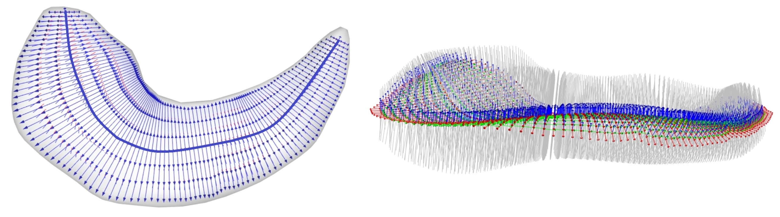
Figure 2: A dss-rep of a hippocampus. Left: Discrete skeletal sheet. Right: Skeletal spokes in grey with tails on the skeletal sheet.

The swept skeletal structure is also a form of skeletal structure that is not unique. Therefore, the center curve of a swept region with a swept skeletal structure is also not unique. In fact, as long as the center curve of a swept region satisfies Damon’s criterion of the RCC, it can be bent such that the cross-sections do not intersect within the object. The RCC defines a curvature tolerance for the center curve to ensure the cross-sections do not intersect within the object (Damon, 2008; Ma et al., 2018) (see Figure 24 in SUP). For example, for a 2D GC, the RCC can simply be determined at each point along the center curve based on its normal as $r<\frac{1}{\kappa}$, where $r$ is the object’s width in the direction of the normal, and $\kappa$ is the curve’s curvature. Let us consider an example in 2D to illustrate our approach.

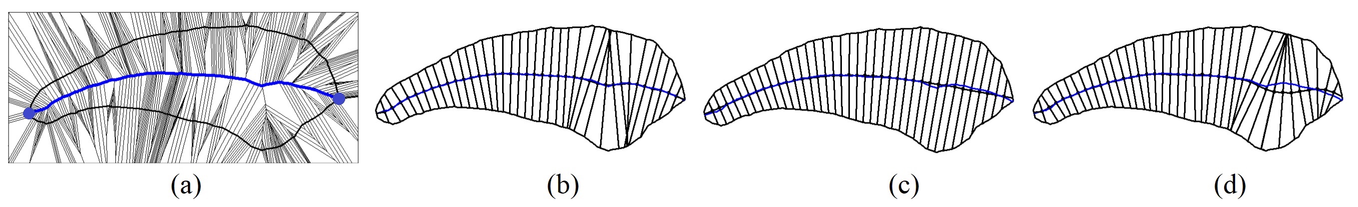
Figure 3: The skeletal structure of a 2D GC. (a) The approximation of the medial axis based on the Voronoi diagram. The CMS is the blue curve connecting the two vertices (blue dots). (b) A model based on a smooth curve very close to the CMS is invalid as it violates the RCC. (c) A valid model based on a slightly relaxed CMS, which is tidy but not highly symmetric. (d) A valid model with high symmetricity. The model is close to violating the RCC.

Assume a 2D GC as depicted in Figure 3 (a). The medial skeleton of the object is calculated as shown in Figure 3 (a) based on the Voronoi diagram (Attali et al., 2009; Dey and Zhao, 2004). The object can be divided in two parts, as discussed in Section 3, resulting in two vertices depicted by blue dots. The CMS of the object is a unique curve (depicted in blue) with no branch or discontinuity connecting the two vertices of the 2D GC. The CMS is a pruned version of the medial skeleton and is unique. Thus, it seems reasonable to construct the swept skeletal structure based on it. However, the CMS is not smooth and has a bumpy structure (specifically at the intersection of the branches). In this example, we cannot consider the CMS or a smooth differentiable curve very close to the CMS as the center curve because they violate the RCC (i.e., the cross-sections intersect within the object because of its high local curvature), as shown in Figure 3 (b). Therefore, the dss-rep cannot be established. However, following Pizer et al. (2013), by relaxing the CMS, the center curve satisfies the RCC, as depicted in Figure 3 (c) and Figure 3 (d). In Figure 3 (c), we slightly relaxed the CMS in the sense that the relaxed version is very close to the CMS. Based on Damon’s discussions, Figure 3 (c) is a valid model even though it is not perfectly symmetric (as the spokes with a common tail position do not need to have equal length). In Figure 3 (d), we increased the flexibility of the model so that it becomes more symmetric, i.e., the center curve is closer to the middle of the cross-sections. However, we observe that the center curve is very close to violating the RCC. Note that defining a perfectly symmetric model with cross-sections normal to the center curve usually is not feasible even if the object has a smooth non-branching medial skeleton (Shani and Ballard, 1984) (see Figure 23 in SUP). Obviously, the structure of Figure 3 (c) is tidier than Figure 3 (d) as the center curve has lower local curvature. In other words, the orientations of adjacent cross-sections in Figure 3 (c) are not significantly different. There is a trade-off between skeletal-symmetry and skeletal-tidiness, and both are crucial factors in defining a model in addition to the volume-coverage. Thus, in Section 6, we introduce an overall score based on these three criteria to measure the goodness of fit within a set of model candidates for the swept skeletal structure.

One conceivable method for fitting a dss-rep into an SlO is to calculate the spine as a curve skeleton (Dey and Sun, 2006) in the first place and define the cross-sections along the spine. However, there are concerns with the curve skeleton. For example, even a smooth curve skeleton may still have branches because there is no criterion that a curve skeleton must be a simple curve. There are approaches for simplifying the curve skeleton to defining a simple curve, for instance, the Laplacian contraction of Au et al. (2008), Mean curvature skeleton of Tagliasacchi et al. (2012), $L1$-medial skeleton of Huang et al. (2013), and skeletonization via local separators of Bærentzen and Rotenberg (2021). However, according to our observations, they fail to offer a suitable spine. In fact, the majority of these methods blindly search for the SlO’s skeleton without considering its important geometric properties, such as the crest and vertices. Moreover, these methods commonly overlook the RCC entirely, as it is not a prerequisite for defining the curve skeleton. Therefore, the spine exhibits unpredictable behavior. For example, it may bend and swing freely inside the object, as discussed in SUP.

By assuming a unique crest for an SlO, the CMS is unique. In this work, we use the CMS to propose a novel dss-rep model fitting. We start by defining the skeletal sheet by relaxing the SlO’s CMS. Then, we use the relaxed CMS to define the spine as a curve located on the skeletal sheet connecting the SlO’s two vertices, as we discuss in Section 4.2. The method we describe ensures that it achieves good correspondence across the population samples based on the uniqueness of the CMS. The method is independent of boundary registration and complies with the definition of SlO. Further, the model fitting procedure is flexible and can be tuned to obtain a tidy and symmetric model. We discuss the tuning based on the essential properties of skeletal-symmetry, tidiness, and the volume of the implied boundary.

To make the analysis alignment independent and to capture the type of local dissimilarities (e.g., protrusion, elongation, etc.), we adapt the idea of locally parameterized ds-rep (LP-ds-rep) suggested by Taheri and Schulz (2022) to introduce locally parameterized dss-rep (LP-dss-rep) by parameterizing the dss-rep based on a tree-like structure of its skeletal sheets equipped with local frames as discussed in Section 5. The structure of this work is as follows.

Section 2 reviews basic terms and provides explicit definitions of a swept region, SlO, skeletal structure, and swept skeletal structure. Section 3 introduces the CMS. Section 4 uses the CMS to propose a dss-rep model fitting procedure based on skeleton flattening using dimensionality reduction methods. Section 5 and Section 6 introduce the LP-dss-rep and discuss the goodness of fit for a proper model based on essential skeletal symmetry and tidiness as well as the volume of the implied boundary. Section 7 demonstrates LP-dss-rep hypothesis testing and classification based on LP-dss-rep Euclideanization. Section 8 compares the LP-ds-rep with the LP-dss-rep based on a set of toy examples and a real data set to discuss the pros and cons of our method. Finally, Section 9 summarizes and concludes the work.

2 Basic terms and definitions

In this section, we review basic terms and definitions regarding skeletal structures.

We consider the set $\Omega\subset\mathbb{R}^{d}$ as a $d$-dimensional object if $\Omega$ is homeomorphic to the $d$-dimensional closed ball, where $d\in\mathbb{N}$. We denote the boundary of $\Omega$ by $\partial\Omega$ and its interior by $\Omega_{in}$, so $\Omega=\Omega_{in}\cup\partial\Omega$. Assume point $\bm{p}\in\Omega_{in}$ and a unit direction $\bm{u}\in\mathbb{S}^{d-1}$, where $\mathbb{S}^{d-1}=\{\bm{x}\in\mathbb{R}^{d}\mid\|\bm{x}\|=1\}$ is the unit $(d-1)$-sphere. Assume $\Omega$ as a 2 or 3-dimensional object. If we start at $\bm{p}$ and move straight forward based on $\bm{u}$, we ultimately reach a boundary point. We call such a straight interior path with starting point $\bm{p}$ and direction $\bm{u}$ a spoke. We denote a spoke based on its positional and directional components by $\bm{s}_{(\bm{p},\bm{u})}$.

We consider the skeletal spokes of $\Omega$ as a set of all non-crossing spokes emanating from its skeleton $M$. The skeletal structure of $\Omega$ is a field of skeletal spokes $U$ on $M$ denoted by $(M,U)$ (see Figures 3 and 4). The medial skeletal structure is one form of skeletal structure where the object’s skeleton is the medial skeleton. The medial skeleton of object $\Omega$ is the set

$$M_{\odot}=\{\bm{p}\in\Omega_{in}\mid\;\lvert\{\bm{q}\in\partial\Omega\mid\,\|\bm{p}-\bm{q}\|=d_{min}(\bm{p},\partial\Omega)\}\rvert_{c}\geq{2}\},$$ (1)

where $d_{min}(\bm{p},\partial\Omega)$ is the minimum Euclidean distance between $\bm{p}$ and $\partial\Omega$, and $\|.\|$ and $\lvert.\rvert_{c}$ represent the Euclidean norm and cardinality, respectively. In other words, $M_{\odot}$ is the center of all maximal (inscribed) spheres bi-tangent (or multi-tangent) to $\partial\Omega$. A medial spoke is a spoke connecting the center of a maximal sphere to its tangency point. The collection of all medial spokes $U_{\odot}=\{\bm{s}_{(\bm{p},\bm{u})}\mid\bm{p}\in{M}_{\Omega}\;\text{and}\;\|\bm{s}_{(\bm{p},\bm{u})}\|=d_{min}(\bm{p},\partial\Omega)\}$ on the medial skeleton $M_{\odot}$ forms the medial skeletal structure $(M_{\odot},U_{\odot})$ (Siddiqi and Pizer, 2008). Figure 4 illustrates the medial skeleton and a few medial spokes of a 2D object.

Figure 4: Illustration of a medial skeleton and maximal spheres. The bold curve is the medial skeleton. The dotted lines are medial spokes.

A swept region is a $d$-dimensional object with a smooth sequence of affine slicing planes along a center curve (not necessarily normal to the center curve) such that cross-sections do not intersect within the object, and each cross-section is a $(d-1)$-dimensional object (Damon, 2008). In other words, the slicing planes sweep the object’s interior and boundary (see Figures 1 and 3).

Let $\Gamma$ be the center curve of the swept region $\Omega$, and let $M$ be the skeleton of $\Omega$. Assume $\Gamma_{(t)}$ as the curve length parameterization of $\Omega$ such that $t\in[0,1]$, where $\Gamma_{(0,1)}$ denotes the curves’ endpoints (Srivastava and Klassen, 2016). Let $\Pi_{(t)}$ be the slicing plane crossing $\Gamma_{(t)}$, and let $\Omega_{(t)}=\Pi_{(t)}\cap\Omega$ be the cross-section at $\Gamma_{(t)}$. Let $U_{(\bm{p})}$ denote the set of skeletal spokes with tails on $\bm{p}\in{M}$. The skeletal structure of $\Omega$ is a swept skeletal structure if, for each $\bm{p}\in{\Omega_{(t)}}\cap{M}$, the $U_{(\bm{p})}\in\Omega_{(t)}$, i.e., all the skeletal spokes with tails on a cross-section are coplanar. Thus, the slicing planes also sweep the object’s skeletal structure (Damon, 2008). We consider an object as a GC if its skeletal structure is a swept skeletal structure and its skeleton $M$ is a smooth open curve. For example, a cylinder is a 3D GC, and an ellipse is a 2D GC, where the skeleton is the major axis and the slicing planes are perpendicular to the center curve (Brady and Asada, 1984; Giblin and Brassett, 1985; Ma et al., 2018).

Following Pizer et al. (2022) and Taheri and Schulz (2022), in this work, we consider an SlO as a swept region with a swept skeletal structure such that each cross-section is a 2D GC, the length of the spine (i.e., the SlO’s center curve) is notably larger than the length of the skeleton of each cross-section. The intersection of the spine with each 2D GC is a point on and approximately at the middle of the 2D GC’s skeleton. The union of the 2D GCs’ boundaries forms the SlO’s boundary, and the union of the 2D GCs’ skeletons forms the SlO’s skeleton, called the skeletal sheet. For instance, any eccentric ellipsoid (i.e., an ellipsoid with unequal principal radii) is an SlO by considering the ellipsoid’s major axis (i.e., the intersection of the first principal axis with the ellipsoid) as the spine and (parallel) slicing planes perpendicular to the spine with cross-sections as ellipses which are 2D GCs. Thus, the skeletal sheet of the ellipsoid is the union of the ellipses’ skeletons, i.e., the intersection of the first principal plane of the ellipsoid with itself.

3 Central medial skeleton

In this section, we discuss the CMS of 2D GCs and SlOs as a subset of their medial skeleton. In Section 4, we use the CMS to fit the SlO’s dss-rep.

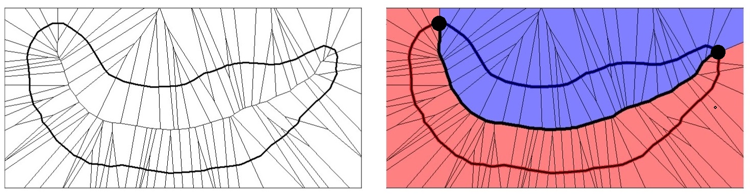
Figure 5: Left: The Voronoi diagram of a 2D GC. Right: The top and bottom parts are depicted as blue and red curves. The two sub-regions are two union polygons associated with the top and bottom parts with the same color. The CMS is the black curve as part of the shared boundary of the union polygons connecting the object vertices.

We know the medial skeleton can be approximated by the Voronoi diagram (Attali et al., 2009). A Voronoi diagram is a geometric structure that partitions a space into regions based on the proximity to a specified set of points called sites. In a Voronoi diagram, each region is a polygon consisting of all the points in the space that are closer to a particular site than to any other site. By assuming the sites as a large number of points uniformly distributed on the object’s boundary, the polygons’ borders located inside the object approximate the medial skeleton (Dey and Zhao, 2004), as depicted in Figure 5 (Left).

Assume $\Omega$ as a 2D GC object with two vertices. The two vertices divide the boundary $\partial\Omega$ into two non-overlapping components, namely top part and bottom part. Each part is a simply connected manifold with no holes or discontinuity. These two parts cover the entire boundary without any gaps. In a discrete sense, $\partial\Omega$ and its two parts can be represented by a set of adjacent points. Thus, each boundary point belongs to only one part, and each part is a set of adjacent points (De Berg, 2000). Let $\partial\hat{\Omega}$ be the discrete form of $\partial\Omega$, and $\partial\hat{\Omega}^{+}$ and $\partial\hat{\Omega}^{-}$ be the top and bottom parts, respectively. Thus, $\partial\hat{\Omega}=\cup\partial\hat{\Omega}^{\pm}$. Assume a box that contains $\partial\hat{\Omega}$. The Voronoi diagram of each part consists of a set of adjacent polygons such that adjacent polygons share a common edge. The union of these adjacent polygons is a union polygon as a connected subset of the box. Therefore, the box (or the embedding space) is partitioned into two sub-regions. Let $\Omega^{+}$ and $\Omega^{-}$ be the intersection of the two sub-regions with $\Omega$ associated with $\partial\hat{\Omega}^{+}$ and $\partial\hat{\Omega}^{-}$. Thus, $\Omega^{+}$ and $\Omega^{-}$ can be seen as two sub-objects, such that $\Omega=\cup\Omega^{\pm}$. The intersection of these sub-objects $\Omega^{+}\cap\Omega^{-}$ defines their shared boundary that we consider as the central medial skeleton (CMS) of $\Omega$.

The CMS can be seen as the locus of the centers of all inscribed spheres bitangent to both parts. In other words, the CMS is a subset of the medial skeleton that is central relative to the $\partial\hat{\Omega}^{+}$ and $\partial\hat{\Omega}^{-}$. This occurs because the distances from any point on the CMS to both the top and bottom parts are equal. Therefore, the CMS is a unique subset of the medial skeleton. Further, the CMS has no branches because it is part of $\partial\Omega^{+}$ (i.e., the boundary of the object $\Omega^{+}$). Also, the CMS has no discontinuity because if it has a discontinuity, it means $\Omega^{+}$ and $\Omega^{-}$ are adjacent, but there is a gap between them. Thus, there is a polygon inside $\Omega$ that its interior does not belong to $\Omega^{+}$ or $\Omega^{-}$, which contradicts the definition of the Voronoi diagram. Figure 5 illustrates the Voronoi diagram and the CMS of a 2D GC.

Figure 6: (a) The top part, the bottom part, and the crest of a caudate are depicted in blue, red, and yellow, respectively. (b) Voronoi diagram of the caudate in two views. (c) Top: Illustration of the two sub-regions in blue and red. Bottom: The sub-regions are separated to provide a better intuition. (d) The CMS is depicted as a black triangle surface.

Similarly, by assuming a unique crest of an SlO as a closed curve (corresponding to the crest of an eccentric ellipsoid), the crest divides the SlO’s boundary into two parts- the top and bottom parts. The Voronoi diagrams of the two parts define two union polyhedrons (i.e., two 3D polygons) as two sub-objects. The CMS of a SlO is the shared boundary of these two sub-objects. Thus, the CMS is a unique subset of the medial skeleton. Analogous to the CMS of a 2D GC, the CMS of an SlO is manifold with no holes or branches. Figure 6 (a) illustrates the top part, the bottom part, and the crest of a caudate nucleus as an SlO. Figure 6 (b) shows the Voronoi diagram of the SlO located in a box. Figure 6 (c) depicts the two sub-regions associated with the top and bottom parts. The sub-regions are also separated to provide a clear intuition about the sub-regions. Figure 6 (d) illustrates the CMS.

4 Fitting swept skeletal structure

In this section, we discuss fitting swept skeletal structures for 2D GCs, and then we generalize the method for SlOs.

We assume the skeleton or the center curve of a 2D GC is a smooth open curve. If we move on the boundary of a 2D GC, the directions of the normals do not change intensively except near the vertices associated with the endpoint of the center curve Siddiqi and Pizer (2008, Ch.8.8). The same discussion is valid for an SlO near the crest (Giblin and Kimia, 2003, 2004; Siddiqi and Pizer, 2008; Fletcher et al., 2004).

Thus, for an SlO, the normal directions of any two close points on each boundary part are not significantly different unless at the area near the crest. Abulnaga et al. (2021) used this property to calculate the crest and the two boundary parts. They considered the discrete boundary and measured the geodesic distance between any two boundary points (to find how far apart they are) and their normal difference. Then, they applied spectral clustering of Ng et al. (2001) (as a binary classification method) to classify the boundary points into the top and bottom parts.

The main idea of our model fitting is to apply Abulnaga’s method to divide the SlO’s boundary, obtain the CMS based on the two boundary parts, fit a smooth manifold representing the skeletal sheet close to the CMS, and finally find the spokes from the skeleton to the boundary such that the obtained skeletal structure is a swept skeletal structure. For better intuition, we start our discussion using a 2D GC, as depicted in Figure 7.

4.1 Fitting a swept skeletal structure to a 2D GC

Assume a 2D GC with two vertices. The objective is to calculate the center curve as an open curve connecting the two vertices and a sequence of slicing planes along the center curve so that the slicing planes do not intersect within the object. To do so, first, we find the top and bottom parts of the object. Then, we calculate the CMS. The CMS is a curve connecting the two vertices. Finally, we relax CMS to define the center curve and slicing planes.

Let $\Omega_{2}$ be a 2D GC with the center curve $\Gamma_{\Omega_{2}}$. Assume $\Gamma_{\Omega_{2}}^{0}$ and $\Gamma_{\Omega_{2}}^{1}$ as the curve’s endpoints corresponding to the two vertices. Also, let $\partial\Omega_{2}^{+}$ and $\partial\Omega_{2}^{-}$ be the top and bottom parts of $\partial\Omega_{2}$, respectively. Thus, $\Gamma_{\Omega_{2}}^{0,1}$ are at the edge of the top and bottom parts. Therefore, to find the $\Gamma_{\Omega_{2}}^{0,1}$ and the CMS of the object, it is sufficient to find the top and bottom parts.

For this purpose, we cluster boundary points into two groups as explained by Abulnaga et al. (2021) with the assumption that the directions of the boundary normals only change significantly around $\Gamma_{\Omega_{2}}^{\pm}$, the same way they behave at the vertices of an ellipse. Abulnaga et al. (2021) defined the affinity matrix $[W]_{i,j}=\exp\{\delta\langle\bm{n}_{i},\bm{n}_{j}\rangle{d_{g}(\bm{x}_{i},\bm{x}_{j})}\}$, where $\bm{n}_{i}$ is the normal vector at the $i$th boundary vertex $\bm{x}_{i}$, $d_{g}$ indicate the geodesics distance and $\delta$ is a penalization parameter to control the local effect of normals’ variation. Therefore, the elements of the affinity matrix reflect the distance between two boundary points and how much their normals are different. Thus, based on spectral clustering of Ng et al. (2001), the sign of the second smallest eigenvectors of the normalized Laplacian $\mathcal{L}=I-D^{\frac{-1}{2}}WD^{\frac{-1}{2}}$ classifies the boundary points into two classes as top and bottom parts that are consistent with the orientation of the normals, where $I$ is the identity matrix, and $[D]_{i,j}=\Sigma_{j}{[W]_{i,j}}$. The same discussion is valid for SlOs (see Figure 8). In this work, we choose $\delta=0.5$ as it usually results in a reasonable crest. In SUP, the boundary division of a caudate is visualized based on different values of $\delta$.

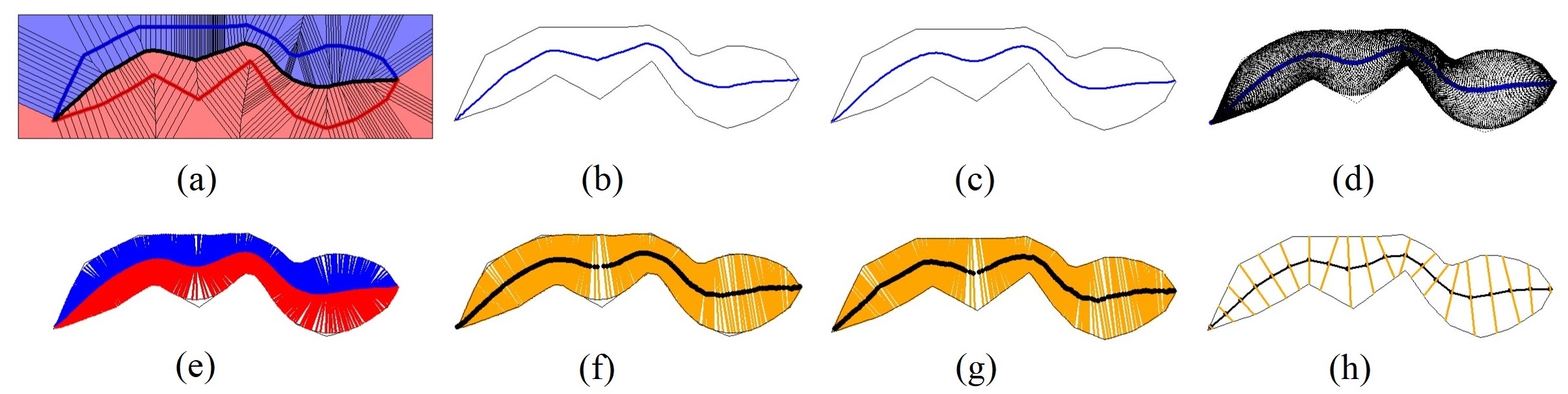
Figure 7: Obtaining the center curve of a 2D GC. (a) Blue and red show the sub-regions associated with the boundary’s top and bottom parts. (b) The CMS. (c) The relaxed CMS. (d) The maximal inscribed circles are centered at the relaxed CMS. The implied boundary is the envelope of the inscribed circles. (e) Up and down skeletal spokes of a large number of points on the relaxed CMS in blue and red. (f) Chordal structure of the implied boundary. (g) Semi-chordal structure of the object. Black dots show the semi-chordal skeleton. (h) The dss-rep of the 2D GC based on the curve length registration.

As discussed in Section 3, by having the top and bottom parts, we can calculate the CMS based on the Voronoi diagram, as shown in Figure 7 (a). The two sub-regions are in blue and red. Figure 7 (b) depicts the CMS, which is not smooth. We relax the CMS by fitting a smooth curve close to it (e.g., by implicit polynomial (Unsalan and Erçil, 1999), principal curve (Hastie and Stuetzle, 1989), nonlinear regression (Ritz and Streibig, 2008), etc.), as depicted in Figure 7 (c). Let $\hat{\Gamma}_{\Omega_{2}}$ be the relaxed CMS. We generate a large number of maximal inscribed circles inside ${\Omega_{2}}$ with a center on $\hat{\Gamma}_{\Omega_{2}}$ as illustrated in Figure 7 (d). Since $\hat{\Gamma}_{\Omega_{2}}$ is continuous, we can consider the envelope of the maximal inscribed spheres as the boundary of an object $\hat{\Omega}_{2}$ such that $\hat{\Gamma}_{\Omega_{2}}$ is the medial skeleton of $\hat{\Omega}_{2}$. We know when the medial skeleton is a smooth open curve, for each medial point $\bm{p}$; there are two spokes at two sides of the medial skeleton with the tail at $\bm{p}$ and tip at the object boundary as

$$\bm{b}=\bm{p}-\mathscr{R}(l)\lvert\frac{d}{dl}{\mathscr{R}(l)}\rvert\bm{t}\pm{\mathscr{R}(l)}\sqrt{1-\lvert\frac{d}{dl}{\mathscr{R}(l)}\rvert^{2}}\bm{n},$$ (2)

where $\bm{n}$ and $\bm{t}$ are normal and tangent vectors of the medial skeleton at $\bm{p}$, and $\mathscr{R}$ is the radius function based on curve length parameterization $l$ such that $\mathscr{R}(l)$ is the radius of the maximal inscribe sphere centered at $\bm{p}$ (Giblin and Kimia, 2003). Therefore, for a large number of medial points, we generate two spokes pointing toward the top and bottom parts as depicted in Figure 7 (e). Note that we can also make the relaxed CMS curvier as long as it produces non-intersecting spokes (similar to Figure 3 (d)).

We consider two top and bottom parts for $\partial\hat{\Omega}_{2}^{\pm}$ based on the endpoints of $\hat{\Gamma}_{\Omega_{2}}$. We call spokes connecting medial points to the $\partial\hat{\Omega}_{2}^{+}$ and $\partial\hat{\Omega}_{2}^{-}$ as up and down spokes, respectively. The relaxed CMS equipped with the spokes as shown in Figure 7 (e) can be seen as the medial representation (m-rep) of the 2D GC if the implied boundary of the spokes approximates the object boundary (Pizer et al., 1999; Fletcher et al., 2004). In other words, $\hat{\Omega}_{2}$ represents $\Omega_{2}$ if the Jaccard index $J(\Omega_{2},\hat{\Omega}_{2})\approx{1}$, where $J(\Omega_{2},\hat{\Omega}_{2})=\frac{\|\Omega_{2}\cap\hat{\Omega}_{2}\|_{A}}{\|\Omega_{2}\cup\hat{\Omega}_{2}\|_{A}}$ and $\|.\|_{A}$ measures the area. In Section 6.1, we discuss the Jaccard index based on the volume coverage for our 3D models.

If we connect the tips of the up and down spokes, we obtain the chordal structure as a set of non-crossing line segments connecting $\partial\hat{\Omega}_{2}^{+}$ and $\partial\hat{\Omega}_{2}^{-}$ as discussed by Giblin and Brassett (1985). Thus, $\hat{\Omega}_{2}$ is a 2D GC with cross-sections defined as the chordal structure of $\hat{\Omega}_{2}$. Note that the chordal skeleton depicted in black in Figure 7 (g) (i.e., the union of the middle of the chords) is slightly different from the medial skeleton of Figure 7 (f) (see (Giblin and Brassett, 1985)). In the next step, we stretch the chords until they reach the actual boundary $\partial\Omega$, as shown in Figure 7 (g). We consider the stretched chords as semi-chords. The semi-chords represent the cross-sections of the 2D GC $\Omega_{2}$, and the curve connecting the middle of the semi-chords, called the semi-chordal skeleton, represents the center curve of $\Omega_{2}$. The semi-chords may intersect somewhere between the implied boundary $\partial\hat{\Omega}_{2}$ and the actual boundary $\partial\Omega_{2}$. In this case, we trim the semi-chords based on the point of intersection. However, the trimming stage can be skipped if the relaxed CMS has low curvature everywhere (because based on the RCC, $r\rightarrow\infty$ when $\kappa\rightarrow 0$). Thus, the semi-chordal structure (i.e., semi-chords plus the semi-chordal skeleton) satisfies the RCC. The implied boundary of the semi-chordal structure (i.e., the envelope of the cross-sections) represents the actual boundary even though they are not exactly the same. Similar to m-rep, a good semi-chordal structure should approximate the actual boundary with the Jaccard index as $\approx 1.0$. The semi-chordal structure can also be used for straightening the 2D GC, as discussed in SUP. Finally, based on the discussion of Srivastava and Klassen (2016) on curve registration, we can choose corresponding semi-chords (e.g., based on curve length registration) across a sample of 2D GCs. In this sense, we have the dss-rep of the 2D GC as shown in Figure 7 (h).

4.2 Fitting a swept skeletal structure to an SlO

For fitting a dss-rep to an SlO, similar to fitting a dss-rep to a 2D GC, we divide $\partial\Omega_{3}$ into the top and bottom parts $\partial\Omega_{3}^{\pm}$. Figure 8 shows the top and bottom parts of a mandible (without coronoid processes), a caudate nucleus, and a hippocampus.

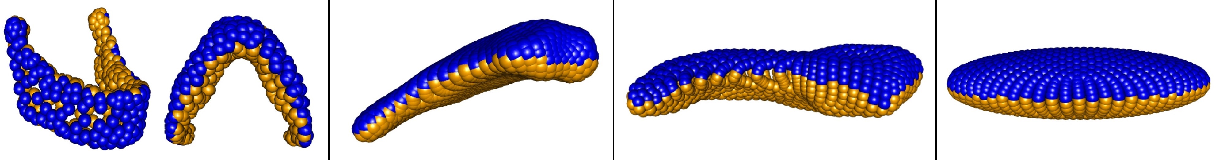
Figure 8: Visualization of SlOs. Blue and yellow indicate the top and bottom parts of a mandible (in two angles), a caudate, a hippocampus, and an ellipsoid from left to right.

We consider the border between $\partial\Omega_{3}^{+}$ and $\partial\Omega_{3}^{-}$ as the crest denoted by $\partial\Omega_{3}^{0}$ as shown in Figure 6 (a). Thus, $\partial\Omega_{3}^{0}$ corresponds to the crest of an eccentric ellipsoid, which is an ellipse, i.e., the intersection of the ellipsoid’s first principal plane with its boundary. Based on $\partial\Omega_{3}^{\pm}$ we obtain the CMS, as depicted in Figure 6 (d) and Figure 9 (Left). We relaxed the CMS by fitting a smooth surface close to it (e.g., based on spline surface fitting (Lee et al., 1997)). We consider the relaxed CMS as the skeletal sheet, as visualized in Figure 9 (Right).

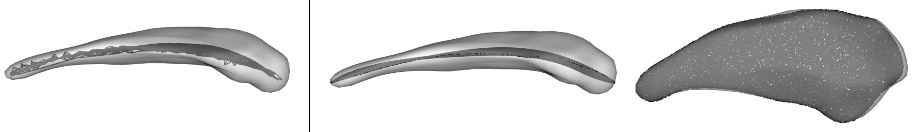
Figure 9: Left: The CMS of a caudate. Right: Two views of the relaxed CMS.

Based on our observations, the skeletal sheet of most brain objects has low curvature everywhere, and its flattened version can be seen as 2D GC with two vertices. We call an SlO with such a skeletal sheet a regular SlO; otherwise, an irregular SlO.

4.2.1 Regular SlO

For fitting the spine (and consequently slicing planes) of a regular SlO, the idea is to flatten the skeletal sheet based on a suitable manifold dimensionality reduction method to become a 2D GC. Then, we fit the center curve of the 2D GC, map the fitted center curve to the skeletal sheet, and consider it as the SlO’s spine. In this sense, the spine is a curve on the skeletal sheet connecting two vertices of the SlO corresponding to the curve connecting the two vertices of the flattened skeletal sheet.

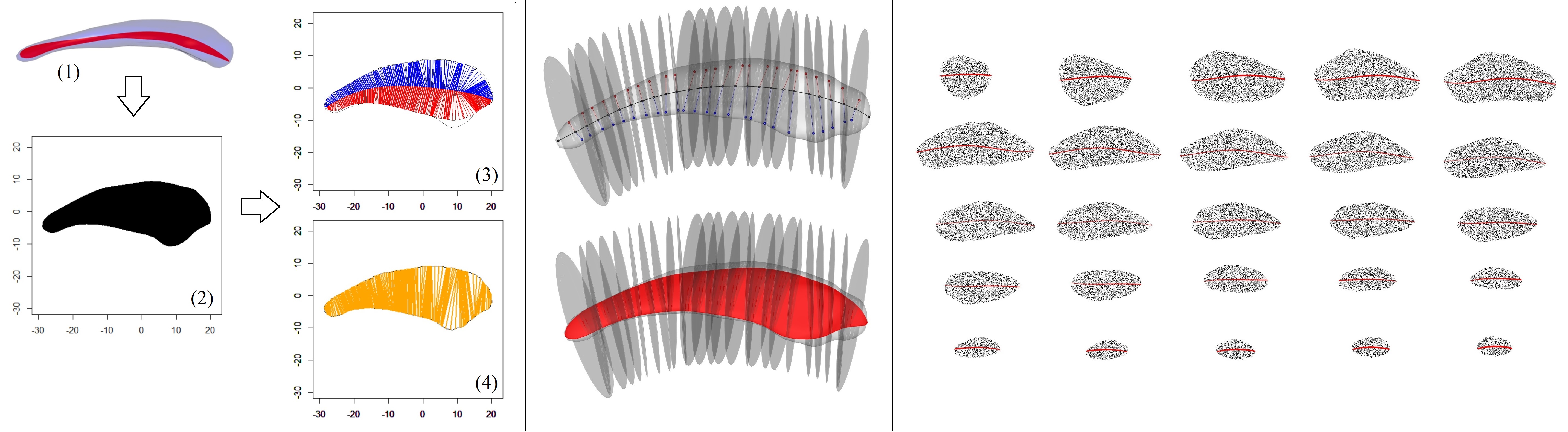
Figure 10: Left: (1) Skeletal sheet of a caudate in red. (2) The PCA projection of the skeletal sheet as a 2D GC. (3) Relaxed CMS and the implied boundary of the 2D GC. (4) Semi-chordal skeletal of the 2D GC. Middle: Visualization of the slicing planes along the spine of a caudate (top) plus the skeletal sheet of the object (bottom). Right: cross-sections and their center curves as the intersection of the slicing planes with the skeletal sheet.

An appropriate dimensionality reduction method preserves the structure of the high-dimensional data properly in the mapped low-dimensional data (Van der Maaten and Hinton, 2008). For example, principal component analysis (PCA) (Hotelling, 1933) is a suitable method when the data has an approximately flat structure relative to the first PCA principal plane (i.e., a plane that is expanded by the first and second eigenvectors originated at the data centroid). In other words, the flattened version of a 3D surface (flattened by PCA) should not be significantly different from its original version. There are various ways to quantify the irregularity or non-flatness of a surface (Bosché and Guenet, 2014; Haitjema, 2017; Mikó, 2021). In this work, we quantify the irregularity based on the maximum local curvature.

For an entirely flat 2D surface, the absolute value of the two principal curvatures (i.e., the eigenvalues of the second fundamental form) are zero everywhere (Pressley, 2013). Assume $M$ as a 2D surface. There is a point on $M$ with absolute average curvature $\kappa_{max}\in[0,\infty)$ such that $\forall\bm{p}\in M$; $\kappa_{\bm{p}}\leq\kappa_{max}$, where $\kappa_{\bm{p}}$ is the average absolute value of the two principal curvatures at $\bm{p}$. Therefore, $\kappa_{max}$ can be assumed as the total curvature of the surface. Thus, the irregularity of $M$ can be strictly quantified as ${2\arctan(\kappa_{max})/\pi\in[0,1]}$. Obviously, $M$ is entirely flat if it has zero irregularity.

Let $\tilde{M}_{\Omega_{3}}$ be the skeletal sheet of $\Omega_{3}$. In this work, we say $\tilde{M}_{\Omega_{3}}$ is semi-flat if its irregularity is less than $0.01$. Let $\tilde{M}_{\Omega_{3}}$ be semi-flat and assume the mapping ${\mathscr{F}:\tilde{M}_{\Omega_{3}}\rightarrow\tilde{M}^{\prime}_{\Omega_{3}}}$ as the orthogonal projection that maps $\tilde{M}_{\Omega_{3}}$ to the PCA first principal plane along the third principal axis. We say the semi-flat $\tilde{M}_{\Omega_{3}}$ is PCA flatable if $\mathscr{F}$ is a diffeomorphism (i.e., $\mathscr{F}$ is a topological preservative bijective mapping between $\tilde{M}_{\Omega_{3}}$ and $\tilde{M}^{\prime}_{\Omega_{3}}$). We consider $\Omega_{3}$ as a regular SlO if $\tilde{M}_{\Omega_{3}}$ is semi-flat, PCA flatable, and $\tilde{M}^{\prime}_{\Omega_{3}}$ can be seen as a 2D GC.

Let $\Omega_{3}$ be a regular SlO, and $\Gamma^{\prime}_{2}$ be the center curve of the embedded 2D GC $\tilde{M}^{\prime}_{\Omega_{3}}$. We consider $\mathscr{F}^{-1}(\Gamma^{\prime}_{2})$ as the spine of $\Omega_{3}$. Also, if $c$ is a semi-chord of $\tilde{M}^{\prime}_{\Omega_{3}}$ we consider $\mathscr{F}^{-1}(c)$ as a non-linear semi-chord of $\tilde{M}_{\Omega_{3}}$. Note that since we apply orthogonal projection, both $c$ and $\mathscr{F}^{-1}(c)$ are located on a plane. Therefore, we can consider these planes as the slicing planes of $\Omega_{3}$. Figure 10 shows the cross-sections of a caudate obtained based on the chordal structure of PCA projection of the skeletal sheet.

As depicted in Figure 11, the semi-chordal skeleton (i.e., the union of middle points of the semi-chords) is usually wavier than the CMS, which is not desirable as it violates the skeleton tidiness that we discuss in Section 6.3. Therefore, we prefer to consider $\Gamma^{\prime}_{2}$ as the relaxed CMS of $\tilde{M}^{\prime}_{\Omega_{3}}$. Further, if the spine (i.e., $\mathscr{F}^{-1}(\Gamma^{\prime}_{2})$) has low curvature everywhere and is not very wavy, we can consider cross-sections perpendicular to the spine based on the spine moving Frenet frame as discussed by Ma et al. (2018). Figure 11 illustrates the spine based on the semi-chordal skeleton (left column), relaxed CMS (middle column), and relaxed CMS such that cross-sections are normal to the spine (right column).

Figure 11: Fitted tree-like structure of the skeletal sheet of a caudate. Left: Slicing planes and the spine are based on chordal structure. Middle: Slicing planes are based on chordal structure, but the spine is based on the relaxed CMS. Right: The spine is based on the relaxed CMS, and the slicing planes are normal to the spine.

4.2.2 Irregular SlO

But what if the skeletal sheet is not semi-flat? Theoretically, the skeletal sheet of an irregular SlO can be bent and twisted with an extremely curvy structure. However, there are irregular SlOs, such as the mandible, whose skeletal sheet has low local curvature. Thus, the skeletal sheet can be properly flattened. We consider such irregular SlOs as treatable SlOs if the flattened skeletal sheet can be seen as a 2D GC. Therefore, analogous to a regular SlO, we consider the inverse map of the center curve of the flatted skeletal sheet, i.e., $\mathscr{F}^{-1}(\Gamma^{\prime}_{2})$ of a treatable SlO as the spine of the object, where $\mathscr{F}$ is a proper embedding. In this case, we define cross-sections normal to the spine.

From initial studies, we found the t-distributed stochastic neighbor embedding (t-SNE) method (Van Der Maaten, 2014) suitable for flattening the skeletal sheet of treatable SlOs. The t-SNE maps high-dimensional data to a lower-dimensional space in such a way that preserves the local structure and relationships between data points as much as possible. It is similar to the SNE of Hinton and Roweis (2002), but instead of using a Gaussian distribution to model these relationships, it employs the t-distribution (Bunte et al., 2012). Figure 12 illustrates the skeletal sheet of a mandible (Left), its t-SNE flattened version as a 2D GC plus the center curve in 2D (Middle), and the mandible with the slicing planes along its spine (Right).

Figure 12: Left: Skeletal sheet of a mandible (without coronoid processes). Middle: Flattened skeletal sheet by t-SNE (left), and center curve of the flattened skeletal sheet (right). Right: Slicing planes of the mandible along the spine.

Often, the complexity of the model fitting problem can be reduced by partitioning an irregular SlO into several regular SlOs. For example, skeletal analysis of a mandible can be based on skeletal models of two segmented hemimandibles (AlHadidi et al., 2012) as regular SlOs (see Figure 14 (d)). However, since the focus of this article is on regular SlOs, we leave further discussions about the generation of slicing planes along the spine of irregular SlOs to our further studies.

5 Parameterization

As Lele and Richtsmeier (2001) discussed, it is crucial for statistical shape analysis that the shape representation is invariant to rigid transformations as shape analysis based on noninvariant shape representation is alignment dependent, while the act of alignment makes the analysis biased and misleading. For example, hypothesis testing to detect local dissimilarity between two groups of objects based on a noninvariant shape representation (e.g., SPHARM-PDM) introduces a large number of false positives and false negatives (Taheri and Schulz, 2022). On the other hand, explaining the type of dissimilarity, such as protrusion, bending, and twisting, is essential for medical researchers. Fortunately, the ds-rep can be parameterized such that the shape representation is invariant and is able to explain the type of dissimilarity. In this regard, Taheri and Schulz (2022) discussed local frames for ds-reps and introduced the LP-ds-rep as an invariant skeletal shape representation based on a tree-like structure of the skeletal sheet. The tree-like structure of LP-dss-rep is established based on the spine and a set of non-intersecting curves emanating from the spine called veins, where the spine and veins are located on the skeletal sheet. The veins connect the spine to the SlO’s crest (analogous to Figure 13). In this sense, the spine and veins define paths for a moving frame on the skeletal sheet. By considering veins as the center curves of the non-intersecting cross-sections, we can define a tree-like structure for the skeletal sheet analogous to LP-ds-rep. Therefore, following the idea of Taheri and Schulz (2022), we parameterize the dss-rep to introduce an invariant shape representation called LP-dss-rep.

5.1 LP-dss-rep

Figure 13: Tree-like structure of the skeletal sheet of a caudate, including local frames in yellow and connection vectors in blue.

Let $\tilde{M}_{\Omega_{3}}$ be the skeletal sheet of the regular SlO ${\Omega_{3}}$. For each point $\bm{p}$ inside $\tilde{M}_{\Omega_{3}}$, there is a line segment based on the semi-chordal structure of the cross-sections that contains $\bm{p}$ with endpoints at $\partial\Omega_{3}^{\pm}$. We consider one up and one down spoke along the line segment with a tail at $\bm{p}$ and tips on ${\partial\Omega_{3}}^{+}$ and ${\partial\Omega_{3}}^{-}$, respectively. Thus, the length of the up and down spokes reflect the local width of ${\Omega_{3}}$, and their difference reflects the local symmetry relative to $\tilde{M}_{\Omega_{3}}$ (i.e., higher differences indicate higher local asymmetry). Assume the middle point of the spine is the skeletal-centroid, as depicted in Figure 13. Thus, the spine can be seen as two curves with the starting point at the skeletal-centroid. Also, the center curve of each cross-section consists of two typically non-straight curves called veins emanating from the spine. Thus, we can consider a vein’s starting point on the spine and its ending point on the SlO’s crest. Since $\bm{p}$ is on the skeletal sheet, it belongs to a curve $\gamma\subset\tilde{M}_{\Omega_{3}}$, where $\gamma$ is the spine or a vein. We define the orthogonal local frame at $\bm{p}$ as $F_{\bm{p}}^{\gamma}=(\bm{n}_{\bm{p}}^{\gamma},\bm{b}^{\gamma}_{\bm{p}},\bm{b}_{\bm{p}}^{\gamma\perp})\in{SO(3)}$, where $\bm{n}_{\bm{p}}$ is normal to $\tilde{M}_{\Omega_{3}}$, $\bm{b}^{\gamma}_{\bm{p}}$ is the velocity vector tangent to $\gamma$, and $\bm{b}_{\bm{p}}^{\gamma\perp}=\bm{n}_{\bm{p}}^{\gamma}\times\bm{b}_{\bm{p}}^{\gamma}$. For points on the intersections of the spines and cross-sections’ center curves (i.e., veins’ starting points), we consider $\gamma$ as the spine. We do not consider frames at the endpoints of the spine and veins as they are at the edge of the skeletal sheet. Therefore, each frame has only one parent frame but up to three children frames. A vector connecting a frame to its parent is called a connection vector, with the tail at the origin of the parent frame and the tip at the origin of the (child) frame. In this sense, the union of the connection vectors has a tree-like structure along the spine from the skeletal-centroid out and along the veins from the spine out. Figure 13 illustrates the tree-like structure of a caudate’s skeletal sheet.

We define an LP-dss-rep as a tuple of geometric object properties (GOPs) of the object as

$$s=(F^{\ast}_{1},...,F^{\ast}_{n_{f}},\bm{v}^{\ast}_{1},...,\bm{v}^{\ast}_{n_{c}},\bm{u}^{\pm\ast}_{1},...,\bm{u}^{\pm\ast}_{n_{f}},v_{1},...,v_{n_{c}},r_{1}^{\pm},...,r^{\pm}_{n_{f}}),$$ (3)

or in the short form $s=(F^{\ast}_{i},\bm{v}^{\ast}_{j},\bm{u}^{\pm\ast}_{i},v_{j},r_{i}^{\pm})_{i,j}$, where $i=1,...,n_{f}$ and ${j=1,...,n_{c}}$, $n_{f}$ is the number of frames, $n_{c}$ is the number of connection vectors, $F^{\ast}_{i}\in{SO(3)}$ is the $i$th frame (orientation) based on its parent coordinate system, $\bm{v}^{\ast}_{j}\in\mathbb{S}^{2}$, and $v_{j}\in{\mathbb{R}^{+}}$ are $j$th connection vector’s direction and length, where the direction is based on the local frame (i.e., a frame that tail of the vector is located on), $\bm{u}^{\pm\ast}_{i}\in\mathbb{S}^{2}$ are the directions of the $i$th up and down spokes based on their local frames, $r_{i}^{\pm}\in{\mathbb{R}^{+}}$ are the lengths of the up and down spokes at the $i$th frame. Thus, an LP-dss-rep lives in a Cartesian product of Euclidean symmetric spaces as

$$\mathbf{S}=(SO(3))^{n_{f}}\times(\mathbb{S}^{2})^{n_{c}+2n_{f}}\times(\mathbb{R}^{+})^{n_{c}+2n_{f}}.$$ (4)

Based on our model fitting $\bm{u}^{+\ast}_{i}=-\bm{u}^{-\ast}_{i}$, we can ignore down spokes’ directions. Thus, we rewrite $s=(F^{\ast}_{i},\bm{v}^{\ast}_{j},\bm{u}^{+\ast}_{i},v_{j},r_{i}^{\pm})_{i,j}$. Further, if the skeletal sheet of a regular SlO has low curvature everywhere, we can consider up and down spokes normal to the skeletal sheet. Therefore, the first frame element at each point represents the direction of its up and down spokes, and we have $s=(F^{\ast}_{i},\bm{v}^{\ast}_{j},v_{j},r_{i}^{\pm})_{i,j}$ and consequently $\mathbf{S}=(SO(3))^{n_{f}}\times(\mathbb{S}^{2})^{n_{c}}\times(\mathbb{R}^{+})^{n_{c}+2n_{f}}$. However, to avoid ambiguity, we stick to the definition of Equation 3 and Equation 4 as they cover both the LP-ds-rep and the LP-dss-rep. Figure 14 depicts the fitted LP-dss-rep to a caudate (a), a hippocampus (b), a mandible (c), and a hemimandible (d).

Figure 14: Fitted LP-dss-rep to a caudate (a), a hippocampus (b), a mandible (c), and a hemimandible (d), including local frames and spokes.

The LP-dss-rep can be used for both shape analysis (i.e., after removing the size) and size-and-shape analysis (i.e., by preserving the size) (Dryden and Mardia, 2016). Since the LP-dss-rep is invariant to rigid transformation, for shape analysis, we remove the scale by dividing the vectors’ lengths by the size of the LP-dss-rep, which we call LP-size (Taheri and Schulz, 2022). The LP-size is the geometric mean of the vectors’ length as

$$\|s\|_{LP}=\exp{(\frac{1}{2n_{f}+n_{c}}(\sum_{j=1}^{n_{c}}\ln(v_{j})+\sum_{i=1}^{n_{f}}\ln(r^{+}_{i})+\sum_{i=1}^{n_{f}}\ln(r^{-}_{i})))}.$$

In Section 8, we analyze real data based on LP-dss-rep shape analysis according to features given earlier.

6 Goodness of fit

In Section 4, we discussed the SlO’s relaxed skeletal structure by fitting the skeletal sheet close to the CMS and defining the spine by fitting a smooth curve close to the relaxed CMS of the flattened skeletal sheet. Thus, we need to explain the level of relaxation. Also, we explored the possibility of choosing different spines based on the chordal skeleton or the relaxed CMS of the flattened sheet (see Figure 11). In addition, we know by definition the swept skeletal structure of an SlO is not unique. Therefore, we need to discuss which model is superior for establishing correspondence and statistical analysis. Obviously, we prefer a model that represents the object such that the implied boundary of the skeletal model approximates the actual boundary. Also, the model should be locally as symmetric as possible because symmetricity is the key element of any skeletal structure. Further, it should be tidy to avoid false positives in the analysis, as we discuss in Section 8. Thus, it is reasonable to search for a superior model with a more tidy and symmetric structure. This can be done by tuning the model fitting procedure based on the flexibility of the curve or surface fitting methods (e.g., by modifying the number of basis functions in B-spline or Fourier expansion (Kokoszka and Reimherr, 2017) or by changing the degree of the polynomial in polynomial regression (Jorgensen, 1993; Montgomery et al., 2015)). In this section, we discuss the goodness of fit of an LP-dss-rep by considering its volume-coverage, skeletal-symmetry, and skeletal-tidiness. Then, in Section 6.4, we discuss our fitting strategy by an example.

6.1 Volume-coverage

Let $s$ be a fitted LP-dss-rep to SlO $\Omega$, where its spokes’ tips are located on $\partial\Omega^{\pm}$, and the endpoints of its veins are located on $\partial\Omega^{0}$. Therefore, we have a point cloud of the spokes’ tips and veins endpoints representing the implied boundary of $s$. We can use this point cloud to generate the implied boundary as a triangular mesh, e.g., by (Pateiro López, 2008), or simply by collapsing the boundary mesh representing $\Omega$ on the point cloud (i.e., by displacing the position of the boundary point $\bm{p}\in\partial\Omega$ to the nearest point of the point cloud). Alternatively, we can use the quadrilateral patches of the skeletal sheet to interpolate spokes and generate the implied boundary as discussed by Han et al. (2006); Liu et al. (2021).

Let $\hat{\Omega}$ be the object generated by the implied boundary. One important factor for the goodness of fit is to see how well $\hat{\Omega}$ approximates $\Omega$. In other words, we prefer a model in which the implied boundary is as close as possible to the actual boundary. Thus, we consider the volume-coverage as the Jaccard index of the model as $J(\Omega,\hat{\Omega})\in[0,1]$, where $J(\Omega,\hat{\Omega})=1$ reflects identical volume. Obviously, we prefer models with higher volume-coverage (see Figure 15).

6.2 Skeletal-symmetry

According to the definition of SlOs, the spine is located on the center curve of each cross-section, approximately at its middle point. The union of the cross-sections’ center curves forms the object’s skeletal sheet. Thus, the skeletal sheet represents the SlO’s skeleton, and the spine can be seen as a nonlinear skeleton of the skeletal sheet (Taheri and Schulz, 2022).

In LP-dss-rep, for each up spoke $\bm{s}_{(\bm{p},\bm{u}^{+})}$ we have a down spoke $\bm{s}_{(\bm{p},\bm{u}^{-})}$ with lengths $r^{+}=\|\bm{s}_{(\bm{p},\bm{u}^{+})}\|$ and $r^{-}=\|\bm{s}_{(\bm{p},\bm{u}^{-})}\|$, respectively. Also, the spine divides the skeletal sheet into two parts, namely, the right side and the left side. For each vein $\nu_{\bm{p}_{s}}^{+}$ at the right side, we have a coplanar vein on the left side $\nu_{\bm{p}_{s}}^{-}$ with a common starting point $\bm{p}_{sp}$ on the spine. Thus, in a symmetric model, we expect $r^{+}\sim{r^{-}}$, and $\|\nu_{\bm{p}_{sp}}^{+}\|_{g}\sim\|\nu_{\bm{p}_{sp}}^{-}\|_{g}$, where $\|.\|_{g}$ measures the curve length. Assume we have $n_{v}$ veins on each side of the spine. Assume vector $\bm{l}^{+}=(r_{1}^{+},...,r_{n_{f}}^{+},\|\nu_{1}^{+}\|_{g},...,\|\nu_{n_{v}}^{+}\|_{g})^{T}$, where $\nu_{t}^{+}$ is the $t$th vein on the right side and $t\in\{1,...,n_{v}\}$. Similarly, assume $\bm{l}^{-}=(r_{1}^{-},...,,r_{n_{f}}^{-},\|\nu_{1}^{-}\|_{g},...,\|\nu_{n_{v}}^{-}\|_{g})^{T}$. For simplicity, we write $\bm{l}^{+}=(l^{+}_{1},...,l^{+}_{n_{f}+n_{v}})^{T}$ and $\bm{l}^{-}=(l^{-}_{1},...,l^{-}_{n_{f}+n_{v}})^{T}$. We define skeletal length as $l_{s}=\sum_{i=1}^{n_{f}+n_{v}}l^{+}_{i}+\sum_{i=1}^{n_{f}+n_{v}}l^{-}_{i}$ and define the weight vector $\bm{w}=(w_{1},...,w_{n_{f}+n_{v}})^{T}$ such that $w_{i}=\frac{l^{+}_{i}+l^{-}_{i}}{l_{s}}$. Then, we define skeletal-symmetry as $\sum_{i=1}^{n_{f}+n_{v}}w_{i}\cdot{f_{i}}$, where $f_{i}=\frac{l^{+}_{i}}{l^{-}_{i}}$ if $l^{-}_{i}\geq{l^{+}_{i}}$ and otherwise ${f_{i}=\frac{l^{-}_{i}}{l^{+}_{i}}}$. Thus, skeletal-symmetry is $\in[0,1]$. If we have a perfect symmetry (i.e., ${\forall{i}:l^{+}_{i}={l^{-}_{i}}}$), then skeletal-symmetry is 1.0.

6.3 Skeletal-tidiness

A model with good volume-coverage and skeletal-symmetry may still be messy. Obviously, we prefer skeletal models that are as tidy as possible for two main reasons. First, untidy models increase the number of false positives and make the analysis misleading because the analysis is a frame-by-frame analysis. Since we consider frames on the skeletal sheet, even a small perturbation on the skeletal sheet violates frame correspondence and hugely affects the results, as we demonstrate by a simple example in Section 8.2.1. Thus, we prefer a model such that the spine and cross-sections’ center curves have the lowest possible curvature. Second, as discussed in Section 1, the center curve at each point must satisfy the RCC.

Let us assume a moving frame $F^{\gamma}$ on an open curve $\gamma$ (representing the spine or a vein) located on the skeletal sheet $M$. In discrete format we assume a sequence of $N+1$ equidistant points $\bm{p}_{0},...,\bm{p}_{N}$ on $\gamma$ and define average perturbation of $\gamma$ as $\zeta(\gamma)=\frac{1}{N}\sum_{i=1}^{N}d_{g}(\bm{q}_{i-1},\bm{q}_{i})\in[0,\frac{\pi}{2}]$, where $\bm{q}_{i}\in\mathbb{S}^{3}$ is the unit quaternion representation of the frame $F_{\bm{p}_{i}}^{\gamma}$, and $d_{g}(\bm{x},\bm{y})=\arccos(\lvert\bm{x}^{T}\bm{y}\rvert)$ is the first quadrant geodesic distance (Huynh, 2009). Thus, $\zeta(\gamma)$ is the mean integrated rotation of the moving frame along $\gamma$ when $N\rightarrow{\infty}$.

Assume a discrete skeletal sheet $M$ with a spine $\gamma_{s}$, spinal points $\bm{p}_{0},...,\bm{p}_{N+1}$, and $N$ cross-sections’ center curves $\{\gamma_{i}\}_{i=1}^{N}$ such that $\gamma_{s}\cap\gamma_{i}=\bm{p}_{i}$. We know $\forall{i}:$ $\bm{n}_{\bm{p}_{i}}^{\gamma_{s}}=\bm{n}_{\bm{p}_{i}}^{\gamma_{i}}$. We define the degree of rotation of the $i$th cross-section relative to the spine by $d_{r}(\gamma_{s},\gamma_{i})=d_{g}(\bm{b}_{\bm{p}_{i}}^{\perp\gamma_{s}},\bm{b}_{\bm{p}_{i}}^{\gamma_{i}})$. Finally, the average perturbation of the skeletal sheet $M$ is defined as

$$\zeta^{\dagger}(M)=\frac{2}{(2N+1)\pi}\left(\zeta({\gamma_{s}})+\sum_{i=1}^{N}\zeta({\gamma_{i}})+\sum_{i=1}^{N}d_{r}(\gamma_{s},\gamma_{i})\right)\in[0,1),$$

and the average tidiness of $M$ as $1-\zeta^{\dagger}(M)$. Thus, the average tidiness of the ellipsoid’s skeleton is 1.0 if the spine is the ellipsoid’s major axis, and the cross-sections (with straight center curves) are normal to the spine, i.e., $\forall{i}:d_{r}(\gamma_{s},\gamma_{i})=0$.

In practice, we need the skeletal sheet as tidy as possible. Thus, it is reasonable to consider $\zeta(\gamma)=\frac{2}{\pi}\max\{d_{g}(\bm{q}_{i-1},\bm{q}_{i})\}_{i=1}^{N}$ and consequently define strict tidiness as $1-\zeta^{\ddagger}(M)$ to judge a model based on its most disordered element, where $\zeta^{\ddagger}(M)=\frac{2}{\pi}\max\{\zeta(\gamma_{s}),\max\{\zeta(\gamma_{i})\}_{i=1}^{N},\max\{d_{r}(\gamma_{s},\gamma_{i})\}_{i=1}^{N}\}$. We define the goodness of fit score as the multiplication of volume-coverage, skeletal-symmetry, and (average or strict) tidiness. In this sense, a model is superior if its score is closer to 1.0.

6.4 Example

The flexibility of our method comes from fitting the skeletal sheet $\tilde{M}_{\Omega_{3}}$ and the center curve of the flattened skeletal sheet $\Gamma^{\prime}_{2}$. Although it is possible to define a standard approach to make the fitting procedure straightforward by, for example, fitting $\tilde{M}_{\Omega_{3}}$ using the B-spline surface fitting of Lee et al. (1997) and fitting $\Gamma^{\prime}_{2}$ using the principal curve fitting of Hastie and Stuetzle (1989), such a standard approach might not be flexible enough to generate distinct LP-dss-reps for an SlO. Therefore, in this work, we prefer to use polynomial regression (PR). Thus, by changing the PR degree from 1 to $n$ (where we consider $n\leq{7}$), we can fit $n\times{n}$ different LP-dss-reps to an SlO. Then, we select the best model based on the goodness of fit. We leave a detailed discussion about choosing the best curve or surface fitting method (from various available methods such as implicit polynomial (Unsalan and Erçil, 1999), nonlinear regression (Ritz and Streibig, 2008), etc.) for our future studies.

Figure 15 depicts 5 (from 49) fitted LP-dss-reps to a hippocampus at the top row and their corresponding implied boundary at the bottom row in blue. The PR degrees for fitting the $\tilde{M}_{\Omega_{3}}$ and $\Gamma^{\prime}_{2}$ are shown in Table 1. Note that the boundary division and, consequently, the CMS for all five samples are the same. For the fit #1 we have a straight line segment as the spine on a perfectly flat skeletal sheet. Although the model is perfectly tidy, its volume-coverage and skeletal-symmetry are weak, resulting in a low model score; see Table 1, where score 1 is based on average tidiness and score 2 is based on strict tidiness.

By adding more flexibility to the spine and the skeletal sheet, we obtained models #2-5. The best skeletal-symmetry and score 1 value belong to model #5. However, as it is obvious from Figure 15 (5), we have a few sudden changes in spinal frames (i.e., cross-sections with high rotation degrees), which reduces the strict tidiness. In contrast, based on score 2, model #3 is the winner as it has good volume-coverage ($\approx 90\%$), skeletal-symmetry ($\approx 87\%$), and strict tidiness ($\approx 90\%$) as we do not observe any extreme changes in frame rotations.

Figure 15: Top row: Fitted LP-dss-reps with parameters given in Table 1. Bottom: Implied boundary in blue.

Table 1: Goodness of fit.

Fit	PR degrees $\tilde{M}_{\Omega_{3}}$, $\Gamma^{\prime}_{2}$	Volume-coverage	skeletal-symmetry	Average tidiness $\zeta^{\dagger}$	Strict tidiness $\zeta^{\ddagger}$	Score 1	Score 2
#1	1, 1	0.812	0.724	1	1	0.588	0.588
#2	3, 4	0.877	0.883	0.969	0.861	0.750	0.667
#3	4, 4	0.890	0.873	0.973	0.890	0.756	0.692
#4	4, 5	0.876	0.861	0.972	0.870	0.733	0.656
#5	7, 7	0.878	0.894	0.971	0.735	0.762	0.577

7 Hypothesis testing

One of the main objectives of LP-dss-rep analysis is to detect dissimilarities between two groups of objects. We explain hypothesis testing for LP-ds-reps similar to LP-dss-reps (Taheri and Schulz, 2022). To do so, in this section, we discuss global and partial LP-dss-rep hypothesis testing based on LP-dss-rep Euclideanization. In addition to the hypothesis testing, LP-dss-rep classification is explained in SUP.

Let $\bm{q}^{\ast}_{i}\in\mathbb{S}^{3}$ be the unit quaternion representation of the $i$th frame (Huynh, 2009). From Equation 3 and Equation 4 we have $s=(\bm{q}^{\ast}_{i},\bm{v}^{\ast}_{j},\bm{u}^{\pm\ast}_{i},v_{j},r_{i}^{\pm})_{i,j}$ and $\mathbf{S}=(\mathbb{S}^{3})^{n_{f}}\times(\mathbb{S}^{2})^{n_{c}+2n_{f}}\times(\mathbb{R}^{+})^{n_{c}+2n_{f}}$, where $\mathbb{S}^{3}$ is the space of local frames based on their unit quaternion representations. Therefore, for a population of LP-dss-reps, we have $n_{c}+3n_{f}$ sets of spherical data (on $\mathbb{S}^{2}$ and $\mathbb{S}^{3}$) and $n_{c}+2n_{f}$ sets of positive real numbers. The spherical data can be Euclideanized by principal nested spheres (PNS) (Jung et al., 2012) or for reducing the computational cost by projecting data to the tangent space (that we use in this work) as discussed by (Kim et al., 2020). Given the mapping $\mathscr{F}:\mathbb{S}^{d}\rightarrow{\mathbb{R}^{d}}$, $s^{e}=(\mathscr{F}(\bm{q}^{\ast}_{i}),\mathscr{F}(\bm{v}^{\ast}_{j}),\mathscr{F}(\bm{u}^{\pm\ast}_{i}),\log{v_{j}},\log{r_{i}^{\pm}})_{i,j}$ is the Euclideanized version of $s$ from Equation 3 that lives on the product space $(\mathbb{R}^{3})^{n_{f}}\times(\mathbb{R}^{2})^{n_{c}+2n_{f}}\times(\mathbb{R}^{+})^{n_{c}+2n_{f}}$.

Now, assume $A=\{{s^{e}_{A}}_{m}\}_{m=1}^{N_{1}}$ and $B=\{{s^{e}_{B}}_{m}\}_{m=1}^{N_{2}}$ are two groups of Euclideanized LP-dss-reps (or LP-ds-rep) of sizes $N_{1}$ and $N_{2}$. We can consider the vectorized version of LP-dss-reps in the feature space (see classification in SUP) and design a global test to compare $A$ and $B$ as two multivariate distributions. Or we can consider LP-dss-reps as tuples and can compare the two populations of tuples element-wise to detect locational dissimilarities, as discussed by Taheri and Schulz (2022).

7.1 Global test

Let $\mu_{A}$ and $\mu_{B}$ be the means of the sets $A$ and $B$, respectively. For the global test, we test $H_{0}:\mu_{A}=\mu_{B}$ versus $H_{0}:\mu_{A}\neq\mu_{B}$. Since the feature space is a high dimensional space, we apply direction projection permutation (DiProPerm) (Wei et al., 2016) with distance weighted discriminator (DWD) (Marron et al., 2007).

7.2 Partial test

The main objective of LP-dss-rep is to detect local dissimilarities. Thus, we design partial hypothesis tests on the GOPs (of Equation 3). Basically, when the result of the global test shows significant dissimilarities, we apply partial tests to detect and explain local dissimilarities.

Let $n_{t}$ be the total number of GOPs. To test GOPs’ mean difference, we design $n_{t}$ partial tests. Let $\mu_{A}(k)$ and $\mu_{B}(k)$ be the observed sample mean of the $k$th GOP from $A$ and $B$, respectively. The partial test is ${H_{0k}:\mu_{A}(k)=\mu_{B}(k)}$ versus ${H_{1k}:\mu_{A}(k)\neq\mu_{B}(k)}$, where $k\in\{1,...,n_{t}\}$. For the partial test, we can apply Hotelling’s T² test with normality assumption or permutation test. Finally, we need to control false positives by methods such as the family wise error rate of Bonferroni (1936) or the false discovery rate (FDR) of Benjamini and Hochberg (1995) (BH).

8 Evaluation

The proposed LP-dss-rep is evaluated in comparison to the available LP-ds-rep that is based on the fitting method of Liu et al. (2021) based on visual inspection and statistical analysis.

8.1 Visual inspection

Figure 16: Toy example for comparing the LP-ds-rep (top row) and the LP-dss-rep (bottom row) of SlOs. Bold blue points are the spines’ endpoints.

For the visual inspection, first, we start with a few toy examples. To design the toy examples, we slightly deform an ellipsoid to make an SlO as a reference object, as illustrated in column (b) of Figure 16. The reference object can be seen as an arm. By bending the reference object with different degrees of bending at the elbow, we make two other SlOs, as depicted in columns (c) and (d). To obtain LP-ds-reps, we used the SlicerSALT toolkit (Vicory et al., 2018). Apparently, by increasing the degree of bending, the LP-ds-rep (i.e., top row) fails to define a good correspondence as the spine does not show enough flexibility to bend according to the degree of bending we impose on the reference object. Also, the structure of the skeletal sheet becomes more and more chaotic. A possible explanation could be the poor boundary registration or the effect of boundary deformation on the skeletal sheet. In contrast to the LP-ds-rep, we can see the structure of the skeletal sheet in the LP-dss-rep is tidier as depicted in the bottom row of Figure 16. Also, the spine shows more flexibility, such that the endpoints of the spines (depicted by bold blue points) are located at the points corresponding to the vertices of the ellipsoid.

Figure 17: Fitted LP-ds-rep (Left) and LP-dss-rep (right) in a hippocampus in two angles.

Analogous to the toy examples, we can see the same issues of the LP-ds-rep on real data. Figure 17 illustrates the LP-ds-reps of hippocampus in two angles with the LP-ds-rep (left), and the LP-dss-rep (right). It seems the spine provides a better description of the SlO center curve in LP-dss-rep.

8.2 Statistical analysis

For the statistical analysis, we start with a simulation of a toy example before analyzing real data.

8.2.1 Toy example

We design a very simple example by simulating two groups of fifty ellipsoids based on randomly generated principal radii such that the ellipsoids of the first group are perfectly symmetric. In contrast, in the second group, there is a small protrusion on the boundary, as illustrated in Figure 18 (a). Figure 18 (d) and (e) show the results of the partial tests from Section 7.2 on the fitted LP-ds-reps and LP-dss-reps, respectively. Although both methods point to the area where we expect to see the difference, the LP-dss-rep reflects the dissimilarity more accurately based on the length of the top spokes in the critical region. In fact, the LP-ds-rep introduces more significant GOPs such that we may conclude that the left part of the two groups is totally different. The reason is that there is a perturbation of the skeletal sheet caused by the boundary deformation, as depicted in Figure 18 (b). In comparison, LP-dss-reps show more resistance against the protrusion and thus better correspondence among the skeletal sheets of the two groups (see Figure 18 (c)). The reason is that the relaxed CMS is less sensitive to boundary protrusion.

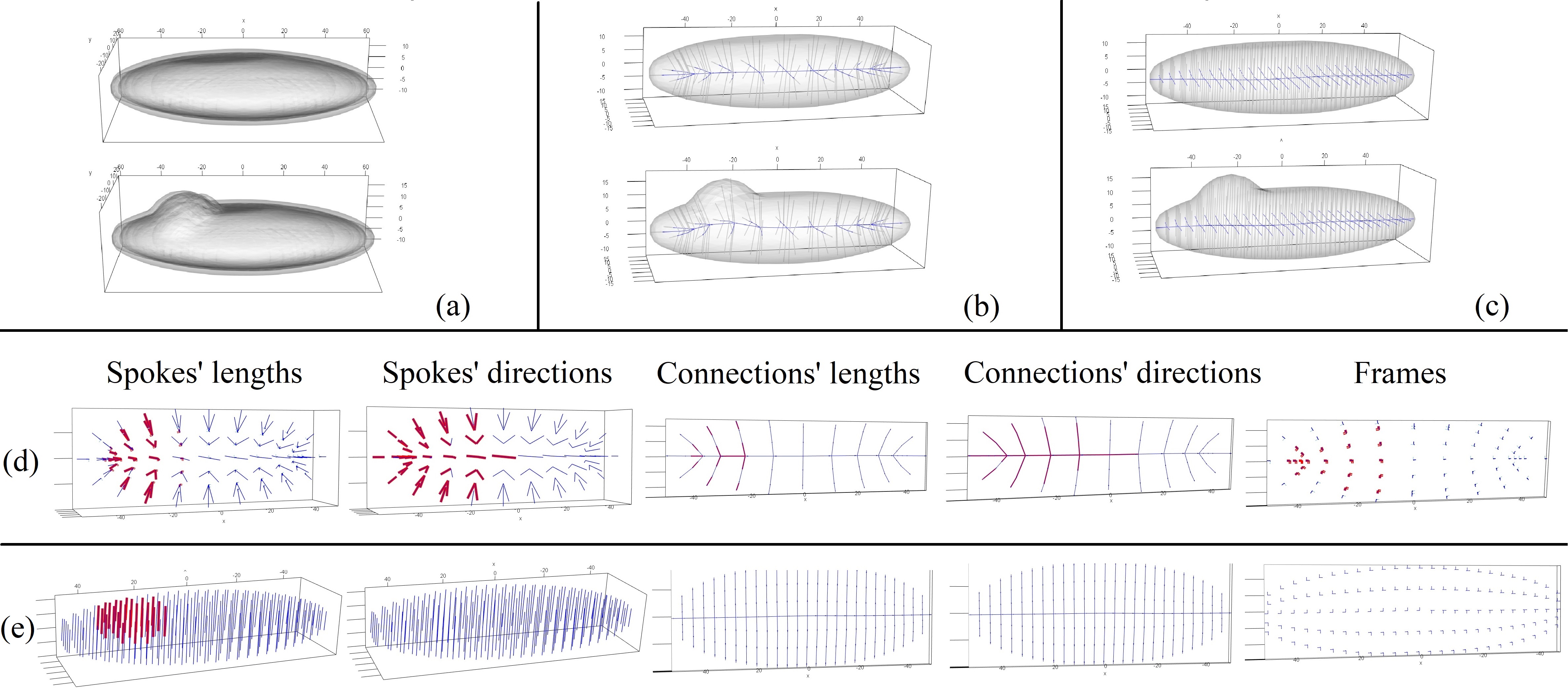
Figure 18: (a) Two groups of simulated ellipsoids with and without boundary protrusion. (b) and (c) LP-ds-rep and LP-dss-rep of two samples from each group. (d) and (e) results of the partial tests on LP-ds-rep and LP-dss-rep, respectively. Red indicates significant GOPs.

8.2.2 Real data

For the statistical analysis, we compare the left hippocampus of 182 patients with early Parkinson’s disease (PD) with the left hippocampus of 108 healthy people as a control group (CG). The data is provided by the Stavanger University Hospital (https://helse-stavanger.no) and the ParkWest study (http://parkvest.no). For this, LP-dss-reps are fitted to the hippocampi of both populations and compared with global and partial hypothesis tests as described in Section 7.1 and Section 7.2 to evaluate if there are differences between the two populations.

Global test

Figure 19 depicts the result of the global test based on DiProPerm. The $p$-value is less than $0.001$ for LP-dss-reps and $0.103$ for LP-ds-reps. Thus, given a significance level of $\alpha=0.05$, PD and CG are statistically significantly different based on LP-dss-reps. Notably, LP-dss-reps have a better performance compared to LP-ds-reps based on the higher Z-score (6.54 vs. 1.32), which indicates that the data are more separated for LP-dss-reps. This might be the effect of the above-described stiffness of LP-ds-reps. In other words, generated LP-ds-reps are relatively similar to each other, which is also reflected in the classification results as discussed in SUP.

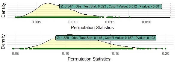
Figure 19: DiProPerm plots of LP-dss-rep (top) and LP-ds-rep (bottom).

Partial tests

The partial tests are illustrated in Figure 20. Both the LP-ds-rep and the LP-dss-rep show significant differences in the spinal connection vectors. The LP-dss-rep introduces fewer significant connection vectors’ directions and frames’ orientations. This behavior supports our conclusion about the skeletal sheet from the toy example.

Figure 20: Partial tests. Red indicates significant GOPs. Results based on the LP-dss-rep (Top) and the LP-ds-rep (Bottom) before and after BH $p$-value adjustment in the first and second rows, respectively. Significant level $\alpha=0.05$ and FDR=0.1.

9 Conclusion

In this work, we introduced a novel model of discrete swept skeletal representation for SlOs called the LP-dss-rep. The LP-dss-rep is designed to support good correspondence between a population of objects, which is important for statistical shape analysis. The fitting is based on dividing the SlO’s surface into two parts, obtaining a skeletal sheet based on the relaxed central medial skeleton, and finding a tree-like structure of the skeletal sheet by the act of mapping and inverse mapping between $\mathbb{R}^{3}$ and $\mathbb{R}^{2}$. The LP-dss-rep is more flexible in comparison with the currently available skeletal model, namely LP-ds-rep. To have a standard measure for choosing the best LP-dss-rep, we introduced goodness of fit criteria based on volume-coverage, skeletal-symmetry, and skeletal-tidiness. The superiority of LP-dss-rep in hypothesis testing over the available LP-ds-rep was demonstrated by visual inspection and statistical analysis on two sets of toy examples and real data. This suggests that by having a proper goodness of fit in a population, the LP-dss-rep provides fewer significant GOPs and a better description of local dissimilarities.

Supplementary Material

SPHARM-PDM correspondence

As depicted in Figure 21, SPHARM-PDM fails to define a good correspondence between the boundary of an ellipsoid and the bent versions of it, as the vertices of the ellipsoid do not correspond to the vertices of the objects.

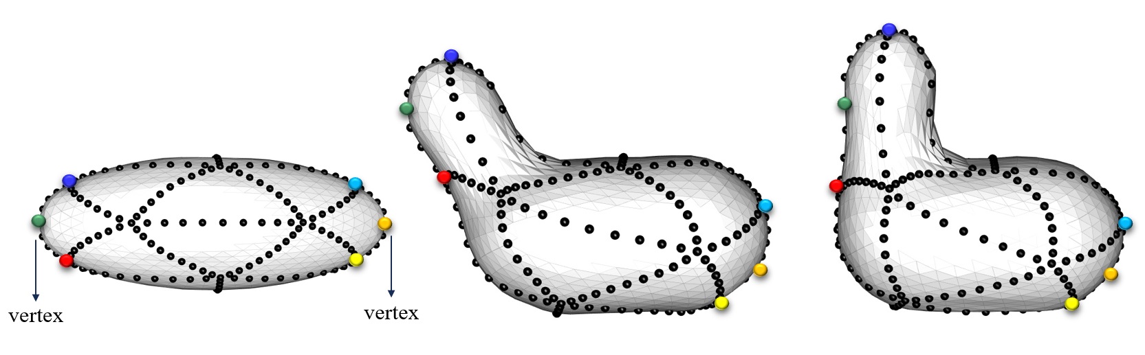
Figure 21: SPHARM-PDM correspondence. Points with the same color are in correspondence.

Choosing $\delta$ for the affinity matrix

Choosing the value of $\delta$ that defines the affinity matrix can slightly change the boundary division. However, based on our observation for most of the objects of our study, $\delta=0.5$ is a reasonable choice. Figure 22 depicts the boundary division of a caudate based on $\delta$ as 0.1, 0.2, 0.5, 0.8, and 0.9, from left to right, respectively

Figure 22: From left to right, the boundary divisions are based on $\delta$ as 0.1, 0.2, 0.5, 0.8, and 0.9, respectively.

Normality versus symmetricity

Figure 23: (a) Cross-sections are normal to the medial skeleton. The RCC is violated. (b) Cross-sections are normal to the center curve, but the center curve is not medial. (c) Cross-sections are not normal to the center curve, but the center curve as the chordal axis traverses the cross-section’s middle points.

In this section, we use Figure 23 (which is similar to Figure 3 of (Shani and Ballard, 1984)) to show even if a 2D GC has a non-branching smooth medial skeleton defining a perfectly symmetric model with normality condition is not feasible. In Figure 23 (a), the cross-sections are normal to the medial skeleton, but the RCC is violated. In Figure 23 (b), cross-sections are normal to the center curve, but the center curve does not meet the middle of the cross-sections. Thus, the model is not symmetric. The model of Figure 23 (c) is perfectly symmetric as the center curve is the chordal skeleton. However, the cross-sections are not normal to the chordal skeleton.

Importance of the RCC

In this section, we provide an illustration to show the importance of the RCC in defining the spine of a swept skeletal structure. Figure 24 depicts two swept skeletal structures of a hippocampus. In Figure 24 (Right), the RCC is satisfied by the spine while in Figure 24 (Left) the RCC is violated. While the spines in both figures exhibit notable similarity, it becomes apparent that defining the spine solely as a curve positioned in the middle of the object is insufficient without considering the RCC.

Figure 24: Left: The RCC is violated. A few cross-sections are intersected within the object. Right: The RCC is satisfied.

Issues with the curve skeleton

There are available methods for calculating the spine of SlOs as a curve skeleton. The curve skeleton, as defined by Dey and Sun (2006), is unique but typically has a branching structure. Based on our experiences, most of the recent methods for pruning and smoothing the curve skeleton, such as Laplacian contraction of Au et al. (2008), mean curvature skeleton of Tagliasacchi et al. (2012), $L1$-medial skeleton of Huang et al. (2013), and skeletonization via local separators of Bærentzen and Rotenberg (2021); Bærentzen et al. (2023)) are more or less suitable for tube-like objects with circular cross-sections. But, they do not provide a suitable spine for slabular objects. The primary issue is that almost all of these methods blindly search for the curve skeleton without considering important boundary properties, such as the crest. We believe a proper spine should be on the skeletal sheet, connecting the SlO’s vertices together, and be relatively in the middle of the cross-sections’. Based on our observations, the mentioned methods do not provide such a spine, even for simple SlOs. In addition, they entirely ignore the RCC. The RCC is not a prerequisite for calculating the curve skeleton because the curve skeleton does not necessarily represent the center curve of a swept region. However, the RCC is vital for defining the center curve of a swept region (see Figure 24). Based on our observations, the curve skeleton exhibits unpredictable behavior inside an SlO. For example, it bends and swings freely inside the object. Therefore, defining corresponding skeletal structures based on the curve skeleton is highly questionable.

For a better intuition, we provide a very simple example to discuss the issue based on skeletonization via local separators of Bærentzen and Rotenberg (2021); Bærentzen et al. (2023). In simple words, the method searches for closed rings called local separators on the boundary. The center points of local separators define the skeleton. Figure 25 shows the spine of two SlOs with smooth boundaries. The obtained spines are based on the PyGEL library (https://www2.compute.dtu.dk/projects/GEL/PyGEL). The spine of each object is not satisfactory as it is non-smooth and perturbed. By considering a smooth version of the spine as depicted by a black curve, the spine still suffers from critical issues. It seems the spine swings and bends freely towards the left parts of the objects. Probably the reason is that the algorithm detects the local separator as the blue curve rather than the yellow curve. On the other hand, the spine violates the RCC.

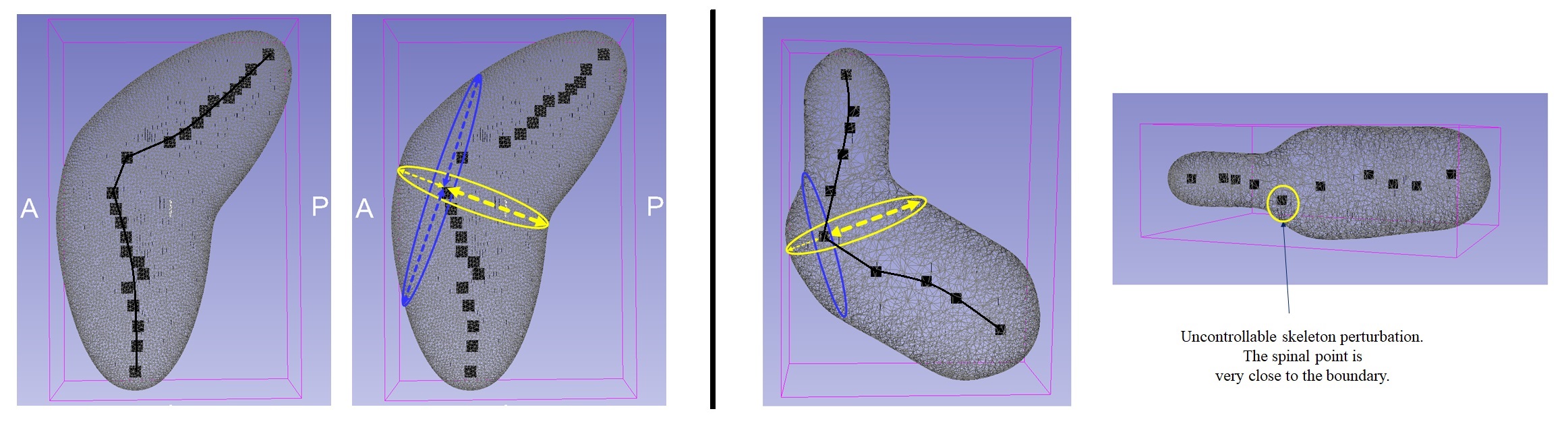
Figure 25: Visualisation of the spine of two SlOs based on the local separator skeleton. The black curve represents the smooth version of the spine. The spines of both objects are bent and swung toward the left side of the objects.

2D GC straightening

As depicted in Figure 26, we can use the chordal structure of a 2D GC to straighten an object. Let $\{c_{i}\}_{i=1}^{n}$ be $n$ consecutive chords (i.e., cross-sections) with points $\{\bm{p}_{i}\}_{i=1}^{n}$, such that $\forall{i}$; $\bm{p}_{i}$ is the middle of $c_{i}$. Let $\|c_{i}\|$ be the length of the $i$th chord. To accomplish the object straightening we use a sequence of points $\{\bm{p}^{\prime}_{i}\}_{i=1}^{n}$ corresponding to $\{\bm{p}_{i}\}_{i=1}^{n}$ on a straight line $\ell$ such that $\forall{i,j}$, $\|\bm{p}^{\prime}_{i}-\bm{p}^{\prime}_{j}\|=d_{g}(\bm{p}_{i},\bm{p}_{j})$, and line segments $\{c^{\prime}_{i}\}_{i=1}^{n}$ corresponding to $\{c_{i}\}_{i=1}^{n}$ such that $\forall{i}$, $c^{\prime}_{i}$ is perpendicular to $\ell$, the middle of $c^{\prime}_{i}$ is on $\ell$, and $\|c^{\prime}_{i}\|=\|c_{i}\|$.

Figure 26: Illustration of 2D GC straightening based on its chordal structure.

Classification

For classification, we follow the idea of composite PNS (CPNS) Pizer et al. (2013). We normalize and vectorize the Euclideanized LP-dss-reps (or LP-ds-reps). Thus, the feature space becomes $\mathbb{R}^{2n_{c}+9n_{f}}$ (or $\mathbb{R}^{2n_{c}+9n_{f}+1}$ in case we consider scaled LP-dss-reps and include the LP-size). In this sense, the problem becomes a binary classification problem of two groups of vectors that can be solved by, e.g., support vector machine (SVM)(Noble, 2006).

For the classification of the real data from Section 7, we applied different standard binary classification methods including k nearest neighbor (KNN), SVM with linear and radial kernels, and naive Bayesian (NB) classification. Further, we applied 10-fold cross-validation to evaluate the accuracy, specificity, and sensitivity of the outcomes based on Cohen’s kappa (Cohen, 1960) as shown in Table 2. As we expected, the classification based on both LP-ds-rep and LP-dss-rep is not promising because, basically, we do not expect to observe separable local distributions at the early stages of PD. However, overall, it seems that the LP-dss-rep has a better performance compared to the LP-ds-rep according to both accuracy and Cohen’s kappa.

Table 2: LP-ds-rep classification based on 10-fold cross-validation.

Classes	Model fitting	Assessment	Classification methods
			KNN	SVM-linear	SVM-radial	NB
PD & CG	LP-ds-rep	Accuracy	0.60	0.55	0.63	0.57
		Kappa	0.10	0.05	0.06	0.14
	LP-dss-rep	Accuracy	0.63	0.63	0.60	0.61
		Kappa	0.18	0.17	0.10	0.11

Declarations

Ethical Approval

Not applicable.

Competing interests

The authors declare no competing interests.

Authors’ contributions

Mohsen Taheri is the first author and writer of the manuscript. Jörn Schulz and Stephen Pizer have supervised the project. All authors read and approved the final manuscript.

Funding

Not applicable

Availability of data and materials

Implementation of the manuscript’s methodology is available as R scripts on https://github.com/MohsenTaheriShalmani/LP-dss-rep. Due to limited permission to share the Parkwest data, we only provide R code for producing toy examples and synthetic data in the repository.

References

- \bibcommenthead
- Abulnaga et al. (2021) Abulnaga, S.M., E.A. Turk, M. Bessmeltsev, P.E. Grant, J. Solomon, and P. Golland. 2021. Volumetric parameterization of the placenta to a flattened template. IEEE Transactions on Medical Imaging 41(4): 925–936 .
- AlHadidi et al. (2012) AlHadidi, A., L.H. Cevidanes, B. Paniagua, R. Cook, F. Festy, and D. Tyndall. 2012. 3d quantification of mandibular asymmetry using the spharm-pdm tool box. International journal of computer assisted radiology and surgery 7(2): 265–271 .
- Apostolova et al. (2012) Apostolova, L., G. Alves, K.S. Hwang, S. Babakchanian, K.S. Bronnick, J.P. Larsen, P.M. Thompson, Y.Y. Chou, O.B. Tysnes, H.K. Vefring, et al. 2012. Hippocampal and ventricular changes in parkinson’s disease mild cognitive impairment. Neurobiology of aging 33(9): 2113–2124 .
- Attali et al. (2009) Attali, D., J.D. Boissonnat, and H. Edelsbrunner. 2009. Stability and computation of medial axes-a state-of-the-art report. Mathematical foundations of scientific visualization, computer graphics, and massive data exploration 1: 109–125 .
- Au et al. (2008) Au, O.K.C., C.L. Tai, H.K. Chu, D. Cohen-Or, and T.Y. Lee. 2008. Skeleton extraction by mesh contraction. ACM transactions on graphics (TOG) 27(3): 1–10 .
- Bærentzen and Rotenberg (2021) Bærentzen, A. and E. Rotenberg. 2021. Skeletonization via local separators. ACM Transactions on Graphics (TOG) 40(5): 1–18 .
- Bærentzen et al. (2023) Bærentzen, J.A., R.E. Christensen, E.T. Gæde, and E. Rotenberg. 2023. Multilevel skeletonization using local separators. arXiv preprint arXiv:2303.07210 1: 1–32 .
- Ballard and Brown (1982) Ballard, D. and C. Brown. 1982. Representations of three-dimensional structures. Computer Vision 1: 264–311 .
- Benjamini and Hochberg (1995) Benjamini, Y. and Y. Hochberg. 1995. Controlling the false discovery rate: a practical and powerful approach to multiple testing. Journal of the Royal statistical society: series B (Methodological) 57(1): 289–300 .
- Blum et al. (1967) Blum, H. et al. 1967. A transformation for extracting new descriptors of shape. Models for the perception of speech and visual form 19(5): 362–380 .
- Bonferroni (1936) Bonferroni, C. 1936. Teoria statistica delle classi e calcolo delle probabilita. Pubblicazioni del R Istituto Superiore di Scienze Economiche e Commericiali di Firenze 8: 3–62 .
- Bosché and Guenet (2014) Bosché, F. and E. Guenet. 2014. Automating surface flatness control using terrestrial laser scanning and building information models. Automation in construction 44: 212–226 .
- Brady and Asada (1984) Brady, M. and H. Asada. 1984. Smoothed local symmetries and their implementation. The International Journal of Robotics Research 3(3): 36–61 .
- Bunte et al. (2012) Bunte, K., S. Haase, M. Biehl, and T. Villmann. 2012. Stochastic neighbor embedding (sne) for dimension reduction and visualization using arbitrary divergences. Neurocomputing 90: 23–45 .
- Cohen (1960) Cohen, J. 1960. A coefficient of agreement for nominal scales. Educational and psychological measurement 20(1): 37–46 .
- Damon (2003) Damon, J. 2003. Smoothness and geometry of boundaries associated to skeletal structures i: Sufficient conditions for smoothness. In Annales de l’institut Fourier, Volume 53, pp. 1941–1985.
- Damon (2008) Damon, J. 2008. Swept regions and surfaces: Modeling and volumetric properties. Theoretical Computer Science 392(1-3): 66–91 .
- De Berg (2000) De Berg, M. 2000. Computational geometry: algorithms and applications. Springer Science & Business Media.
- Dey and Sun (2006) Dey, T.K. and J. Sun 2006. Defining and computing curve-skeletons with medial geodesic function. In Symposium on geometry processing, Volume 6, pp. 143–152.
- Dey and Zhao (2004) Dey, T.K. and W. Zhao. 2004. Approximating the medial axis from the voronoi diagram with a convergence guarantee. Algorithmica 38: 179–200 .
- Dryden and Mardia (1998) Dryden, I. and K. Mardia. 1998. Statistical Shape Analysis. Wiley Series in Probability & Statistics. Wiley.
- Dryden and Mardia (2016) Dryden, I. and K. Mardia. 2016. Statistical Shape Analysis: With Applications in R. Wiley Series in Probability and Statistics. Wiley.
- Fletcher et al. (2004) Fletcher, P.T., C. Lu, S.M. Pizer, and S. Joshi. 2004. Principal geodesic analysis for the study of nonlinear statistics of shape. IEEE transactions on medical imaging 23(8): 995–1005 .
- Gamble and Heo (2010) Gamble, J. and G. Heo. 2010. Exploring uses of persistent homology for statistical analysis of landmark-based shape data. Journal of Multivariate Analysis 101(9): 2184–2199 .
- Giblin and Kimia (2004) Giblin, P. and B.B. Kimia. 2004. A formal classification of 3d medial axis points and their local geometry. IEEE Transactions on Pattern Analysis and Machine Intelligence 26(2): 238–251 .
- Giblin and Brassett (1985) Giblin, P.J. and S. Brassett. 1985. Local symmetry of plane curves. The American Mathematical Monthly 92(10): 689–707 .
- Giblin and Kimia (2003) Giblin, P.J. and B.B. Kimia. 2003. On the intrinsic reconstruction of shape from its symmetries. IEEE Transactions on Pattern Analysis and Machine Intelligence 25(7): 895–911 .
- Haitjema (2017) Haitjema, H. 2017. Flatness, pp. 1–6. Berlin, Heidelberg: Springer Berlin Heidelberg.
- Han et al. (2006) Han, Q., S.M. Pizer, and J.N. Damon 2006. Interpolation in discrete single figure medial objects. In 2006 Conference on Computer Vision and Pattern Recognition Workshop (CVPRW’06), pp. 85–85. IEEE.
- Hastie and Stuetzle (1989) Hastie, T. and W. Stuetzle. 1989. Principal curves. Journal of the American Statistical Association 84(406): 502–516 .
- Hinton and Roweis (2002) Hinton, G.E. and S. Roweis. 2002. Stochastic neighbor embedding. Advances in neural information processing systems 15: 1–5 .
- Hotelling (1933) Hotelling, H. 1933. Analysis of a complex of statistical variables into principal components. Journal of educational psychology 24(6): 417 .
- Huang et al. (2013) Huang, H., S. Wu, D. Cohen-Or, M. Gong, H. Zhang, G. Li, and B. Chen. 2013. L1-medial skeleton of point cloud. ACM Trans. Graph. 32(4): 65–1 .
- Huynh (2009) Huynh, D.Q. 2009. Metrics for 3d rotations: Comparison and analysis. Journal of Mathematical Imaging and Vision 35(2): 155–164 .
- Jermyn et al. (2017) Jermyn, I., S. Kurtek, H. Laga, A. Srivastava, G. Medioni, and S. Dickinson. 2017. Elastic Shape Analysis of Three-Dimensional Objects. Synthesis Lectures on Computer Vision. Morgan & Claypool Publishers.
- Jorgensen (1993) Jorgensen, B. 1993. Theory of Linear Models. Chapman & Hall/CRC Texts in Statistical Science. Taylor & Francis.
- Jung et al. (2012) Jung, S., I.L. Dryden, and J. Marron. 2012. Analysis of principal nested spheres. Biometrika 99(3): 551–568 .
- Kim et al. (2020) Kim, B., J. Schulz, and S. Jung. 2020. Kurtosis test of modality for rotationally symmetric distributions on hyperspheres. Journal of Multivariate Analysis 178: 104603 .
- Kokoszka and Reimherr (2017) Kokoszka, P. and M. Reimherr. 2017. Introduction to Functional Data Analysis. Chapman & Hall/CRC Texts in Statistical Science. CRC Press.
- Laga et al. (2019) Laga, H., Y. Guo, H. Tabia, R. Fisher, and M. Bennamoun. 2019. 3D Shape Analysis: Fundamentals, Theory, and Applications. Wiley.
- Lee et al. (1997) Lee, S., G. Wolberg, and S.Y. Shin. 1997. Scattered data interpolation with multilevel b-splines. IEEE transactions on visualization and computer graphics 3(3): 228–244 .
- Lele and Richtsmeier (2001) Lele, S.R. and J.T. Richtsmeier. 2001. An invariant approach to statistical analysis of shapes. Chapman and Hall/CRC.
- Liu et al. (2021) Liu, Z., J. Hong, J. Vicory, J.N. Damon, and S.M. Pizer. 2021. Fitting unbranching skeletal structures to objects. Medical Image Analysis 70: 102020 .
- Ma et al. (2018) Ma, R., Q. Zhao, R. Wang, J.N. Damon, J.G. Rosenman, and S.M. Pizer 2018. Skeleton-based generalized cylinder deformation under the relative curvature condition. In PG (Short Papers and Posters), pp. 37–40.
- Marron et al. (2007) Marron, J.S., M.J. Todd, and J. Ahn. 2007. Distance-weighted discrimination. Journal of the American Statistical Association 102(480): 1267–1271 .
- Mendelson (2012) Mendelson, B. 2012. Introduction to Topology: Third Edition. Dover Books on Mathematics. Dover Publications.
- Mikó (2021) Mikó, B. 2021. Assessment of flatness error by regression analysis. Measurement 171: 108720 .
- Montgomery et al. (2015) Montgomery, D., E. Peck, and G. Vining. 2015. Introduction to Linear Regression Analysis. Wiley Series in Probability and Statistics. Wiley.
- Ng et al. (2001) Ng, A., M. Jordan, and Y. Weiss. 2001. On spectral clustering: Analysis and an algorithm. Advances in neural information processing systems 14: 849–856 .
- Noble (2006) Noble, W.S. 2006. What is a support vector machine? Nature biotechnology 24(12): 1565–1567 .
- Pateiro López (2008) Pateiro López, B. 2008. Set estimation under convexity type restuctions. Univ Santiago de Compostela.
- Pizer et al. (1999) Pizer, S.M., D.S. Fritsch, P.A. Yushkevich, V.E. Johnson, and E.L. Chaney. 1999. Segmentation, registration, and measurement of shape variation via image object shape. IEEE transactions on medical imaging 18(10): 851–865 .
- Pizer et al. (2020) Pizer, S.M., J. Hong, J. Vicory, Z. Liu, J. Marron, H.y. Choi, J. Damon, S. Jung, B. Paniagua, J. Schulz, et al. 2020. Object shape representation via skeletal models (s-reps) and statistical analysis, Riemannian Geometric Statistics in Medical Image Analysis, 233–271. Elsevier.
- Pizer et al. (2013) Pizer, S.M., S. Jung, D. Goswami, J. Vicory, X. Zhao, R. Chaudhuri, J.N. Damon, S. Huckemann, and J. Marron. 2013. Nested sphere statistics of skeletal models, Innovations for Shape Analysis, 93–115. Springer.
- Pizer et al. (2022) Pizer, S.M., J. Marron, J.N. Damon, J. Vicory, A. Krishna, Z. Liu, and M. Taheri. 2022. Skeletons, object shape, statistics. Frontiers in Computer Science 4: 842637 .
- Pressley (2013) Pressley, A. 2013. Elementary Differential Geometry. Springer Undergraduate Mathematics Series. Springer London.
- Ritz and Streibig (2008) Ritz, C. and J. Streibig. 2008. Nonlinear Regression with R. Use R! Springer New York.
- Schulz (2013) Schulz, J. 2013. Statistical Analysis of Medical Shapes and Directional Data. Ph. D. thesis, UiT Norges arktiske universitet.
- Schulz et al. (2016) Schulz, J., S.M. Pizer, J. Marron, and F. Godtliebsen. 2016. Non-linear hypothesis testing of geometric object properties of shapes applied to hippocampi. Journal of Mathematical Imaging and Vision 54(1): 15–34 .
- Shani and Ballard (1984) Shani, U. and D.H. Ballard. 1984. Splines as embeddings for generalized cylinders. Computer Vision, Graphics, and Image Processing 27(2): 129–156 .
- Siddiqi and Pizer (2008) Siddiqi, K. and S. Pizer. 2008. Medial Representations: Mathematics, Algorithms and Applications. Computational Imaging and Vision. Springer Netherlands.
- Srivastava and Klassen (2016) Srivastava, A. and E. Klassen. 2016. Functional and Shape Data Analysis. Springer Series in Statistics. Springer New York.
- Styner et al. (2006) Styner, M., I. Oguz, S. Xu, C. Brechbühler, D. Pantazis, J.J. Levitt, M.E. Shenton, and G. Gerig. 2006. Framework for the statistical shape analysis of brain structures using spharm-pdm. The insight journal 1(1071): 242 .
- Tagliasacchi et al. (2012) Tagliasacchi, A., I. Alhashim, M. Olson, and H. Zhang 2012. Mean curvature skeletons. In Computer Graphics Forum, Volume 31, pp. 1735–1744. Wiley Online Library.
- Taheri and Schulz (2022) Taheri, M. and J. Schulz. 2022. Statistical analysis of locally parameterized shapes. Journal of Computational and Graphical Statistics 0(ja): 1–28 .
- Turner et al. (2014) Turner, K., S. Mukherjee, and D.M. Boyer. 2014. Persistent homology transform for modeling shapes and surfaces. Information and Inference: A Journal of the IMA 3(4): 310–344 .
- Unsalan and Erçil (1999) Unsalan, C. and A. Erçil 1999. A new robust and fast implicit polynomial fitting technique. In Proc. Int’l Conf. Mechatronics and Machine Vision in Practice (M2VIP’99), pp. 1–8.
- Van Der Maaten (2014) Van Der Maaten, L. 2014. Accelerating t-sne using tree-based algorithms. The Journal of Machine Learning Research 15(1): 3221–3245 .
- Van der Maaten and Hinton (2008) Van der Maaten, L. and G. Hinton. 2008. Visualizing data using t-sne. Journal of machine learning research 9(11): 2579–2605 .
- Van Kaick et al. (2011) Van Kaick, O., H. Zhang, G. Hamarneh, and D. Cohen-Or 2011. A survey on shape correspondence. In Computer graphics forum, Volume 30, pp. 1681–1707. Wiley Online Library.
- Vicory et al. (2018) Vicory, J., L. Pascal, P. Hernandez, J. Fishbaugh, J. Prieto, M. Mostapha, C. Huang, H. Shah, J. Hong, Z. Liu, et al. 2018. Slicersalt: Shape analysis toolbox. In Shape in Medical Imaging: International Workshop, ShapeMI 2018, Held in Conjunction with MICCAI 2018, Granada, Spain, September 20, 2018, Proceedings, pp. 65–72. Springer.
- Wei et al. (2016) Wei, S., C. Lee, L. Wichers, and J. Marron. 2016. Direction-projection-permutation for high-dimensional hypothesis tests. Journal of Computational and Graphical Statistics 25(2): 549–569 .