Additivity of quantum capacities in simple non-degradable quantum channels

Abstract

Quantum channel capacities give the fundamental performance limits for information flow over a communication channel. However, the prevalence of superadditivity is a major obstacle to understanding capacities, both quantitatively and conceptually. Examples of additivity, while rare, provide key insight into the origins of nonadditivity and enable our best upper bounds on capacities. Degradable channels, which have additive coherent information, are some of the only channels for which we can calculate the quantum capacity. In this paper we construct non-degradable quantum channels that nevertheless have additive coherent information and therefore easily calculated quantum capacity. The first class of examples is constructed by generalizing the Platypus channel introduced by Leditzky et al. The second class of examples, whose additivity follows from a conjectured stability property, is based on probabilistic mixture of degradable and anti-degradable channels.

Introduction.—A central problem in quantum information theory is to determine the capacities of various quantum channels. The quantum capacity is defined as the optimal transmission rate over all possible quantum error-correcting codes such that the decoding errors can vanish in the limit of asymtotically many uses of the channel. It was shown in [1, 2, 3, 4](LSD Theorem) that the quantum capacity of a quantum channel $\mathcal{N}$ is characterized by

$$Q(\mathcal{N})=\lim_{n\to\infty}\frac{1}{n}Q^{(1)}(\mathcal{N}^{\otimes n}),$$ (1)

where

$$Q^{(1)}(\mathcal{N}):=\max_{\rho_{A}}I_{c}(\rho_{A},\mathcal{N})$$ (2)

is the maximal coherent information. By optimizing over product states, one always has super-additivity:

$$Q^{(1)}(\mathcal{N}\otimes\mathcal{M})\geq Q^{(1)}(\mathcal{N})+Q^{(1)}(\mathcal{M})$$ (3)

for arbitrary quantum channels $\mathcal{N},\mathcal{M}$. For arbitrary large $n$ we can have $Q(\mathcal{N})>\frac{1}{n}Q^{(1)}(\mathcal{N}^{\otimes n})$ [5, 6, 7] and furthermore inequality in (3) can be strict [8, 9, 10, 11, 12, 13, 14, 15, 16, 17, 18, 19]. These nonadditivities are the main obstacles to evaluate quantum capacity. We refer to [20] for a review of different types of non-additivity. Below, we will consider two notions of additivity of coherent information. We say that the quantum channel $\mathcal{N}$ has weakly additive coherent information, if $Q^{(1)}(\mathcal{N}^{\otimes n})=nQ^{(1)}(\mathcal{N})$ for all $n$. If equality in (3) holds for any quantum channel $\mathcal{M}$, we say $\mathcal{N}$ has strongly additive coherent information. If it holds only if $\mathcal{M}$ is from some subclass of quantum channels, we say $\mathcal{N}$ has strongly additive coherent information with that class of quantum channels.

It is well-known that for degradable channels [21] and PPT channels [22, 23, 24], the quantum capacity can be single-letter characterized. In other words, they have weakly additive coherent information. Moreover, any degradable channel $\mathcal{N}$ has strongly additive coherent information with respect to degradable channels. However, it remains a pressing challenge to find sufficient and necessary conditions for additivity of coherent information.

The main results of this paper aim to provide examples of non-degradable quantum channels of positive quantum capacity with weak and strong additive coherent information, thus extending the class of quantum channels with additivity property. We also provide informational explanation why it can happen. Our goal is not only to determine the capacities of more quantum channels, but also learn about when non-additivity can arise.

First, we revisit the idea of direct sum channels introduced in [25]. If the dimension of a channel’s input system is greater than or equal to $3$, we can decompose the input system into two orthogonal components. We treat one component as a useless resource which deteriorates the degradability of the quantum channel. At the same time, we ensure the capacity is determined by the restriction on the other component. If the restriction channel is degradable or has additive coherent information, then one can show additivity of coherent information of the original channel. We illustrate the idea by constructing a very simple example, which is generalized from the Platypus channels introduced in [12]. We show that for certain extremal parameter values, the channel is non-degradable yet strong additivity holds. We refer the reader to [26, 27] for similar constructions of non-degradable channels with weakly additive coherent information. We also show the failure of strong additivity if we go beyond that region.

The intricate interplay of additivity and non-additivity for non-degradable channels motivates us to find sufficient conditions for strong additivity in non-degradable channels. In particular, we aim to find conditions for strong additivity in non-degradable qubit channels, where a direct sum structure is impossible. Using the notion of partial orders of quantum channels [28], by weakening the degradability condition, we can show strong additivity of coherent information within this class of quantum channels. In particular, we revisit a sufficient condition for additivity introduced in [29] called informational degradability. As an example, we analyze a simple class of qubit-to-two-qubit channels based on probabilistic mixture of degradable and anti-degradable channels which can be neither degradable nor anti-degradable, but for which this weaker notions of degradability appears to hold.

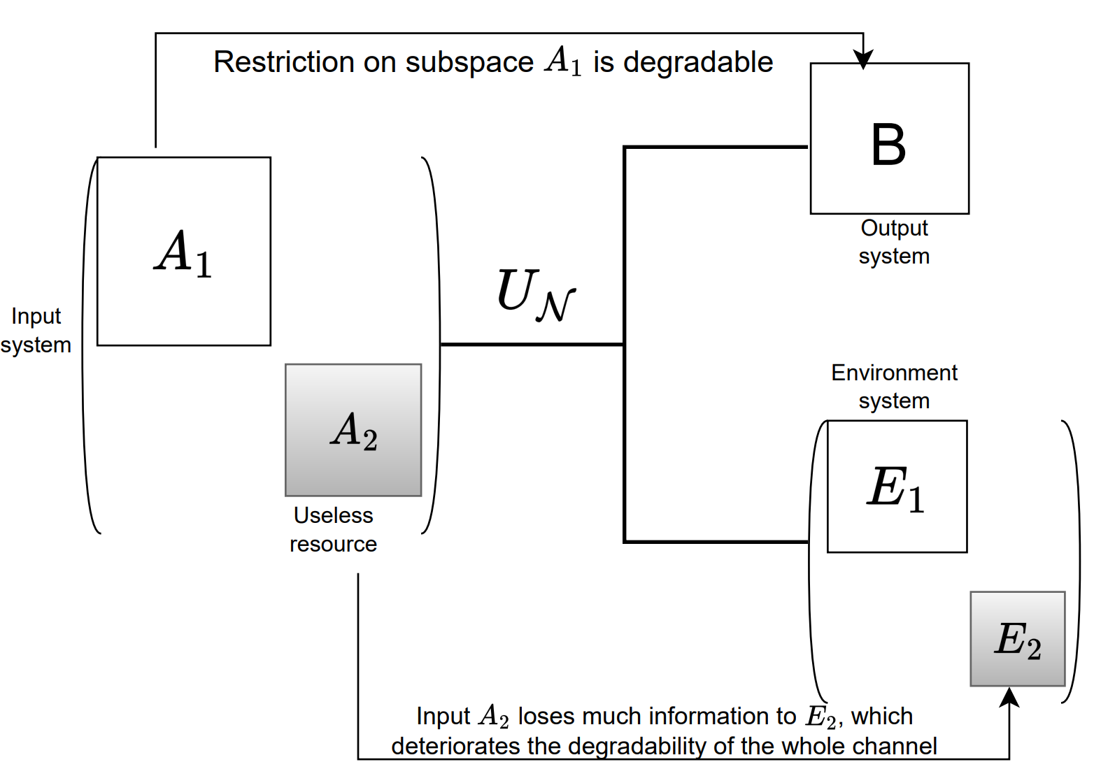
Figure 1: Non-degradable channel with direct sum structure for the input system.

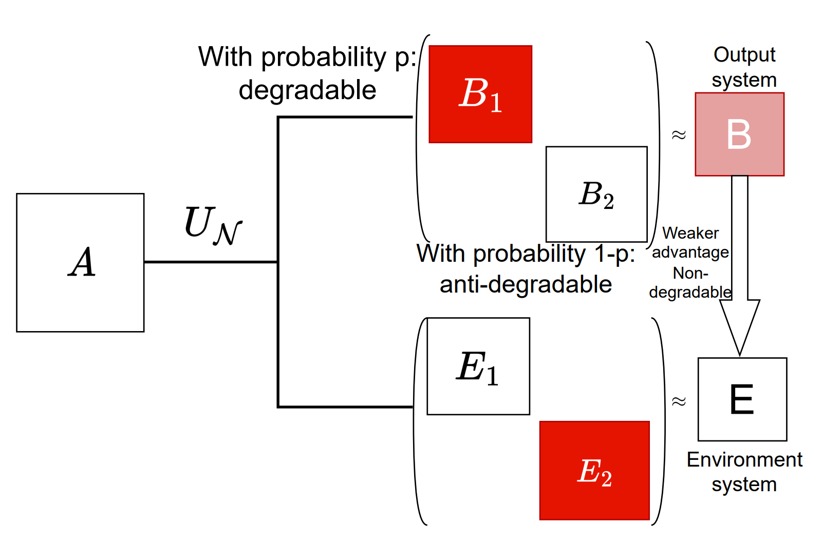
Figure 2: Non-degradable channel using probabilistic mixture of degradable and anti-degradable channels.

Main results.— A quantum channel $\mathcal{N}$ from $\mathcal{H}_{A}$ to $\mathcal{H}_{B}$ can be naturally expressed as an isometry $U_{\mathcal{N}}$ from $\mathcal{H}_{A}$ to $\mathcal{H}_{B}\otimes\mathcal{H}_{E}$ for some environment system $\mathcal{H}_{E}$, followed by a partial trace over the environment system $\mathcal{H}_{E}$: $\mathcal{N}(\rho)=\Tr_{E}(U_{\mathcal{N}}\rho U_{\mathcal{N}}^{{\dagger}})$. Physically, this means that quantum noise arises from sharing quantum information with the environment, which is subsequently lost by tracing out. From this perspective, the complementary channel $\mathcal{N}^{c}(\rho)=\Tr_{B}(U_{\mathcal{N}}\rho U_{\mathcal{N}}^{{\dagger}})$ can be viewed as the signal lost to the environment.

We say that a quantum channel $\mathcal{N}$ is degradable, if there is a quantum channel $\mathcal{D}$ from input system $\mathcal{H}_{B}$ to output $\mathcal{H}_{E}$, such that $\mathcal{D}\circ\mathcal{N}=\mathcal{N}^{c}$. That is, one can process the output system to get all the information about the environment system. Similarly, if there exists a quantum channel $\widetilde{\mathcal{D}}$ from $\mathcal{H}_{E}$ to $\mathcal{H}_{B}$, such that $\widetilde{\mathcal{D}}\circ\mathcal{N}^{c}=\mathcal{N}$, then we say that $\mathcal{N}$ is anti-degradable.

For any input state $\rho_{A}$, we denote $\rho_{B}=\mathcal{N}(\rho_{A}),\rho_{E}=\mathcal{N}^{c}(\rho_{A})$, and the coherent information $I_{c}(\rho_{A},\mathcal{N})$ is defined by

$$I_{c}(\rho_{A},\mathcal{N})=S(\rho_{B})-S(\rho_{E}),$$ (4)

where $S(\rho):=-\Tr(\rho\log\rho)$ is the von Neumann entropy. We denote $S(\rho_{B})$ as $S(B)$ for notational simplicity. The maximal coherent information is defined by $Q^{(1)}(\mathcal{N})=\max_{\rho_{A}}I_{c}(\rho_{A},\mathcal{N})$ and the quantum capacity is the regularized version: $Q(\mathcal{N})=\lim_{n\to\infty}\frac{1}{n}Q^{(1)}(\mathcal{N}^{\otimes n})$. It is well known that strong additivity of coherent information holds within the class of degradable channels [30, Theorem 13.5.1]. Below, we present two different classes of examples which exhibit additivity but they are neither degradable nor anti-degradable.

Generalized Platypus channels.—We first study a simple class of non-degradable and non-anti-degradable channels generalizing the Platypus channels discussed in [12, 13]. Consider an isometry $F_{s,t}:\mathcal{H}_{A}\to\mathcal{H}_{B}\otimes\mathcal{H}_{E}$ with $\rm{dim}\mathcal{H}_{A}=\rm{dim}\mathcal{H}_{B}=\rm{dim}\mathcal{H}_{E}=3$ of the form:

$$F_{s,t}\ket{0}$$ (5)

$$=\sqrt{s}\ket{0}\otimes\ket{0}+\sqrt{1-s-t}\ket{1}\otimes\ket{1}+\sqrt{t}\ket{2}\otimes\ket{2},$$

$$F_{s,t}\ket{1}=\ket{2}\otimes\ket{0},$$

$$F_{s,t}\ket{2}=\ket{2}\otimes\ket{1},$$

where $0\leq s,t\leq 1$ with $s+t\leq 1$. We denote the complementary pair as $(\mathcal{N}_{s,t},\mathcal{N}_{s,t}^{c})$ with $\mathcal{N}_{s,t}(\rho):=\Tr_{E}(F_{s,t}\rho F_{s,t}^{\dagger}),\ \mathcal{N}^{c}_{s,t}(\rho):=\Tr_{B}(F_{s,t}\rho F_{s,t}^{\dagger})$. Note that the above generalization is different from the that in [13, Section X]. The additivity and non-additivity properties are summarized as follows:

• $t\geq\frac{1}{2}$: $\mathcal{N}_{s,t}$ is anti-degradable; $t<\frac{1}{2}$, $\mathcal{N}_{s,t}$ is neither degradable nor anti-degradable.

• For $t<\frac{1}{2}$: if $s+t=1$ or $s=0$, $\mathcal{N}_{s,t}$ has strong additive coherent information with degradable channels and weakly additive coherent information.

• For $t<\frac{1}{2}$: if $s>0,s+t<1$, $\mathcal{N}_{s,t}$ does not have strongly additive coherent information with degradable channels; weak additivity of coherent information is conjectured to be true.

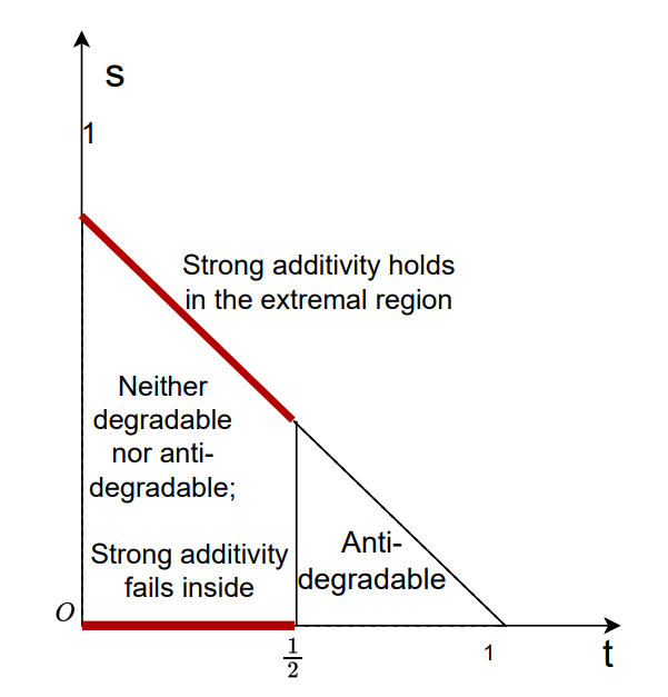
Figure 3: Additivity and non-additivity properties for $\mathcal{N}_{s,t}$

The trick to prove the above result is motivated by [12, 27]. The key observation is that when $s+t=1$(respectively $s=0$), the vector $\ket{2}_{A}$(respectively $\ket{1}_{A}$) can be viewed as a useless resource and the capacity is determined by the restriction on the subspace excluding the useless resource. Moreover, the restriction channel is degradable while the degradability of the original channel is deteriorated by the useless resource, See Figure 1 for an illustration. This construction is similar to the partially coherent direct sum structure introduced in [25] where they require two non-trivial subspace of $\mathcal{H}_{A}$.

When $s>0,s+t<1$, the above structure collapses. The degradability of the restriction channel is destroyed and the restriction channel does not have additivity. In this case, using the fact that the coherent information is still determined by the restriction channel, the $\varepsilon$-log-singularity argument [17] implies the failure of strong additivity of coherent information with simple degradable channels. However, our numerical evidence shows that the weak additivity of coherent information is true. A rigorous argument can be also be given if the spin alignment conjecture is correct, see [13, 31] for the statement and partial progress of spin alignment conjecture.

Probabilistic mixture of degradable and anti-degradable channels.—Previous constructions of non-degradable qudit channels with strong additive coherent information rely heavily on the direct sum structure(with nontrivial subspace) of the input system which requires the dimension of the input system is at least three. One natural question is whether strong additivity of coherent information can still be true for non-degradable channels with no direct sum structure for the input system. In particular, if the input system of a non-degradable quantum channel has dimension two, is it possible to have strong additivity of coherent information? Our analysis shows that it is possible.

Our toy model is given by the following class of qubit-to-two-qubit channels determined by the isometry $V_{p,\eta,\gamma}:\mathcal{H}_{A}\to\mathcal{H}_{B}\otimes\mathcal{H}_{E}$ with $\rm{dim}\mathcal{H}_{A}=2,\ \rm{dim}\mathcal{H}_{B}=\rm{dim}\mathcal{H}_{E}=4$:

$$V_{p,\gamma,\eta}\ket{0} =\sqrt{1-p}\ket{0}\otimes\ket{0}+\sqrt{p}\ket{1}\otimes\ket{1},$$ (6)

$$V_{p,\gamma,\eta}\ket{1} =\sqrt{1-p}(\sqrt{1-\gamma}\ket{2}\otimes\ket{0}+\sqrt{\gamma}\ket{0}\otimes\ket{2})$$

$$+\sqrt{p}(\sqrt{1-\eta}\ket{3}\otimes\ket{1}+\sqrt{\eta}\ket{1}\otimes\ket{3}),$$

for $\gamma,\eta\in[0,1],\ p\in(0,1)$. If we identify $\mathbb{C}^{4}\simeq\mathbb{C}^{2}\otimes\mathbb{C}^{2}$ via $\ket{0}\Leftrightarrow\ket{00},\ket{1}\Leftrightarrow\ket{10},\ket{2}\Leftrightarrow\ket{01},\ket{3}\Leftrightarrow\ket{11}$, the complementary pair of quantum channels $(\Phi_{p,\gamma,\eta},\Phi_{p,\gamma,\eta}^{c})$ determined by $V_{p,\gamma,\eta}$ can be written as a probabilistic mixture of two amplitude damping channels:

$$\Phi_{p,\gamma,\eta}(\rho)=(1-p)\outerproduct{0}{0}\otimes\mathcal{A}_{\gamma}(\rho)+p\outerproduct{1}{1}\otimes\mathcal{A}_{\eta}(\rho),$$ (7)

$$\Phi_{p,\gamma,\eta}^{c}(\rho)=(1-p)\outerproduct{0}{0}\otimes\mathcal{A}^{c}_{\gamma}(\rho)+p\outerproduct{1}{1}\otimes\mathcal{A}^{c}_{\eta}(\rho).$$

We first determine the regions of degradability and anti-degradability and we explore the region where $\Phi_{p,\gamma,\eta}$ is neither degradable nor anti-degradable:

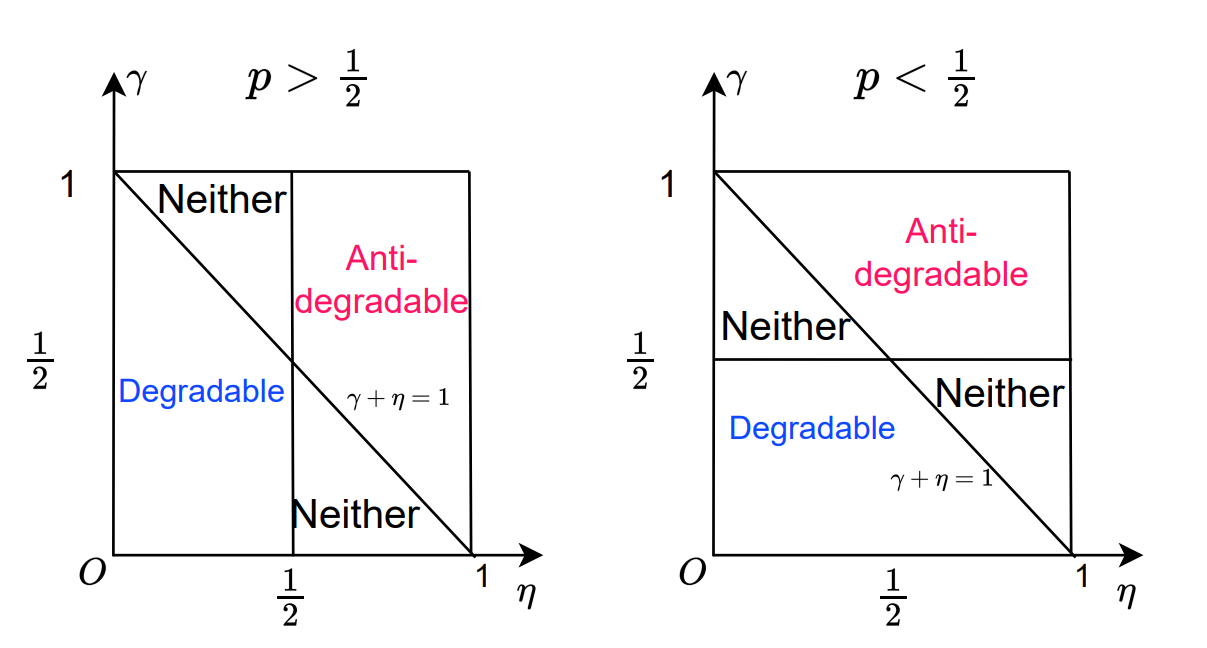
Figure 4: Degradable and anti-degradable regions for probabilistic mixture of two amplitude damping channels defined in (7).

We now argue that in the region where $\Phi_{p,\gamma,\eta}(\rho)$ is neither degradable nor anti-degradable, it can still have weakly additive coherent information. For example, in the region $0<1-\gamma<\eta<\frac{1}{2}$, if we set $p$ close to $1$, then with high probability the quantum channel is the degradable channel $\mathcal{A}_{\eta}$ while the non-zero probability of anti-degradable $\mathcal{A}_{\gamma}$ deteriorates the degradability of the probabilistic mixture of the two. If the probability of the degradable channel is overwhelming, we expect that the output of the channel will have more information about the input than the environment does. Following [29], this would be sufficient for additivity.

To formalize this intution, we introduce the informational advantage of a quantum channel $\mathcal{N}$: given a quantum channel $\mathcal{N}$, the informational advantage of $\mathcal{N}$ at the state $\rho_{VA}$ on the joint system $VA$, is defined as

$$f(\mathcal{N},\rho_{VA})=I(V;B)-I(V;E),$$ (8)

where $I(V;B)=S(B)+S(V)-S(BV)$ is the mutual information of the state $\rho_{VB}=(id_{\mathbb{B}(V)}\otimes\mathcal{N})(\rho_{VA})$. By extending [29], we find that if $f(\mathcal{N},\rho_{VA})\geq 0$ for arbitrary finite dimensional quantum system $V$ and quantum state $\rho_{VA}$, then $\mathcal{N}$ has strongly additive coherent information with degradable channels. It also has weakly additive coherent information, and therefore its quantum capacity is given by $Q^{(1)}(\Phi_{p,\gamma,\eta})$.

In more detail, consider $\Phi_{p,\gamma,\eta}$ with $0<1-\gamma<\eta<\frac{1}{2}$. We know that if $p>\frac{1}{2}$, $\Phi_{p,\gamma,\eta}$ is neither degradable nor anti-degradable. However, we will see that in this region $\Phi_{p,\gamma,\eta}$ may be informationally degradable, which is defined as having $I(V;B)\geq I(V;E)$ for every $\rho_{VA}$. First, note that the mutual information under convex combination of orthogonal states is additive, and denote $f(\gamma,\rho_{VA})=f(\mathcal{A}_{\gamma},\rho_{VA})$. The criterion for informational degradability is $f(\Phi_{p,\gamma,\eta},\rho_{VA})\geq 0$, which is equivalent to

$$pf(\eta,\rho_{VA})\geq(1-p)f(1-\gamma,\rho_{VA}).$$ (9)

This would follow from the the multiplicative stability of informational advantage of amplitude damping channels:
Conjecture: For any $0<\gamma_{1}<\gamma_{2}<\frac{1}{2}$, we have

$$R(\gamma_{1},\gamma_{2}):=\inf_{\rho_{VA},I(V;A)\neq 0}\frac{f(\mathcal{A}_{\gamma_{2}},\rho_{VA})}{f(\mathcal{A}_{\gamma_{1}},\rho_{VA})}>0.$$ (10)

In the supplementary material, we analyze the conjecture in special cases and find that the infimum is achieved when $\rho_{VA}$ is close to its product state $\rho_{V}\otimes\rho_{A}$. The informational advantage $f(\mathcal{A}_{\gamma},\rho_{VA})$ converges to zero if $\rho_{VA}$ converges to its product state. Moreover, our analysis shows that the convergence rate is comparable for $\gamma_{1},\gamma_{2}\in(0,\frac{1}{2})$ when we restrict $\rho_{VA}$ to be pure state. The full generality is left open and we depict it in Figure 5. We see that when $\gamma_{1},\gamma_{2}$ are close, $R(\gamma_{1},\gamma_{2})$ is large; if one of $\gamma_{1},\gamma_{2}$ is close to $0$ or $\frac{1}{2}$, $R(\gamma_{1},\gamma_{2})$ is small which can be explained using the derivative analysis in the supplementary material.

Figure 5: Plot of $R(\gamma_{1},\gamma_{2})$ for $0<\gamma_{1}<\gamma_{2}<\frac{1}{2}$ with $\rm{dim}V=2$.

Assuming this conjecture, there is a threshold probability

$$p^{*}=\frac{1}{1+R(1-\gamma,\eta)}\in(\frac{1}{2},1)$$ (11)

such that if $p\geq p^{*}$, $Eq.~{}(\ref{Eq:MultStab})$ is satisfied and $\Phi_{p,\gamma,\eta}$ is informationally degradable. This can happen in each of the subregions where $\Phi_{p,\gamma,\eta}$ is neither degradable nor anti-degradable and we refer the reader to supplementary material for the whole region.

Conclusion.—In this letter, we discuss two classes of non-degradable quantum channels which exhibit additivity property when we compute the quantum capacity. The first class is generalized from Platypus channels introduced in [13]. For different regions of the parameters determining the quantum channel, we see different types of additivity properties. The second class is given by a probabilistic mixture of amplitude damping channels. We determine the region where the channel is degradable, anti-degradable or neither, and we see that if the probability is above or below a certain threshold, degradability and anti-degradability do not hold, but we argue that a weaker notion of degradability can hold. To determine the threshold probability, we introduce a new quantity called informational advantage and we study its multiplicative stability. A rigorous proof of multiplicative stability would involve finding a quantum dimension bound in the evaluation of $R(1-\gamma,\eta)$ (cf [32, 33]).

Technical Overview

This section serves as an overview of the main results and methods for experts. We provide two parametrized classes of quantum channels, and show that in some parameter regions where the channel is neither degradable nor anti-degradable, the channel can exhibit strong and weak additivity of coherent information. The first class is the so called Generalized Platypus channel, defined by the isometry $F_{s,t}:\mathcal{H}_{A}\to\mathcal{H}_{B}\otimes\mathcal{H}_{E}$ with $\rm{dim}\mathcal{H}_{A}=\rm{dim}\mathcal{H}_{B}=\rm{dim}\mathcal{H}_{E}=3$

$$F_{s,t}\ket{0}=\sqrt{s}\ket{0}\otimes\ket{0}+\sqrt{1-s-t}\ket{1}\otimes\ket{1}+\sqrt{t}\ket{2}\otimes\ket{2},$$ (12)

$$F_{s,t}\ket{1}=\ket{2}\otimes\ket{0},$$

$$F_{s,t}\ket{2}=\ket{2}\otimes\ket{1}.$$

Denote the complementary pair generated by $F_{s,t}$ as $(\mathcal{N}_{s,t},\mathcal{N}_{s,t}^{c})$. To show the degradability and anti-degradability, we apply the composition rule for transfer matrix of super-operators. To be more specific, for a linear super-operator $\mathcal{N}(X)=\sum_{i}A_{i}XB_{i}$, define its transfer matrix as $\mathcal{T}_{\mathcal{N}}:=\sum_{i}B_{i}^{T}\otimes A_{i}$ and we have $\mathcal{T}_{\mathcal{N}_{1}\circ\mathcal{N}_{2}}=\mathcal{T}_{\mathcal{N}_{1}}\mathcal{T}_{\mathcal{N}_{2}}$. Using this trick, we show that if $t\geq\frac{1}{2}$, $\mathcal{N}_{s,t}$ is anti-degradable; if $t<\frac{1}{2}$, $\mathcal{N}_{s,t}$ is neither degradable nor anti-degradable.

Next, we switch our attention to strong additivity property of this channel in the region where $\mathcal{N}_{s,t}$ is neither degradable nor anti-degradable. In fact, we observe that if $s=0$ or $1-s-t=0$, $\mathcal{N}_{s,t}$ satisfies strong additivity with degradable channels and weak additivity. Our key observation is that in those two cases, the vector $\ket{2}_{A}$(respectively $\ket{1}_{A}$) can be viewed as useless resource and the capacity is determined by the restriction on the subspace excluding the useless resource. Moreover, the restriction channel is degradable while the degradability of the original channel is deteriorated by the useless resource. This structure ensures that the channel has additivity property but the degradability property is ruined.

However, if $s>0$ and $1-s-t>0$, the above structure collapses. In fact, one can still show that if $s\geq 1-s-t$ the coherent information of $\mathcal{N}_{s,t}$ is determined by the restriction channel on $\text{span}\{\ket{0},\ket{1}\}$ and similarly if $s\leq 1-s-t$ the coherent information of $\mathcal{N}_{s,t}$ is determined by the restriction channel on $\text{span}\{\ket{0},\ket{2}\}$ via the trick of majorization and Schur concavity of von Neumann entropy. However, the restriction channel fails to be degradable and the additivity fails. Moreover we can show that for erasure channel with probability $\frac{1}{2}$, denoted as $\mathcal{E}_{\frac{1}{2}}$, we have

$$\mathcal{Q}^{(1)}(\mathcal{N}_{s,t}\otimes\mathcal{E}_{\frac{1}{2}})>\mathcal{Q}^{(1)}(\mathcal{N}_{s,t}),\quad s>0,\ 1-s-t>0.$$

The choice of ansatz state achieving the above non-additivity depends on which one of $s$ and $1-s-t$ is larger and is given as follows:

$$\rho_{AA^{\prime}}(\varepsilon)=\begin{cases}r_{*}\outerproduct{00}{00}+(1-r_{*})\ket{\psi_{\varepsilon}},\quad\outerproduct{\psi_{\varepsilon}}{\psi_{\varepsilon}}=\sqrt{1-\varepsilon}\ket{20}+\sqrt{\varepsilon}\ket{11},\ s\geq 1-s-t,\\ r_{*}\outerproduct{00}{00}+(1-r_{*})\ket{\psi_{\varepsilon}},\quad\outerproduct{\psi_{\varepsilon}}{\psi_{\varepsilon}}=\sqrt{1-\varepsilon}\ket{10}+\sqrt{\varepsilon}\ket{21},\ s\leq 1-s-t\end{cases}$$ (13)

where $r_{*}$ is the optimizer for $\mathcal{Q}^{(1)}(\mathcal{N}_{s,t})$ which can be simplified to a single-parameter optimization problem. Then using $\varepsilon$-log-singularity argument, one can show that violation of additivity can happen for $\varepsilon$ sufficiently small.

Our analysis of additivity and non-additivity properties for $\mathcal{N}_{s,t}$ not only provides a new example of non-degradable channel with strong additivity property, but also tells us when non-additivity can happen using the entangled ansatz states.

Our second class of examples is based on weaker notions of degradability. Recall that for degradable channel $\mathcal{N}$ there exists a quantum channel $\mathcal{D}$ such that $\mathcal{D}\circ\mathcal{N}=\mathcal{N}^{c}$. It is natural to ask if there are other partial orders characterizing $\mathcal{N}$ is better than $\mathcal{N}^{c}$. In fact, we revisit a sequence of weaker notions and provide a class of parametrized quantum channels, and in the region where the channel is neither degradable nor anti-degradable, we show evidence that it can be informationally degradable which implies strong additivity.

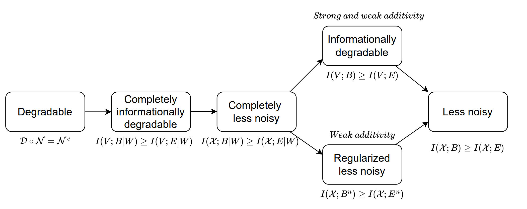
Figure 6: Summary of relations and implications of the weaker notions of degradability, where $V,W$ denote quantum systems and $\mathcal{X}$ denotes a classical system.

Our toy model is given by the isometry $V_{p,\eta,\gamma}:\mathcal{H}_{A}\to\mathcal{H}_{B}\otimes\mathcal{H}_{E}$ with $\rm{dim}\mathcal{H}_{A}=2,\ \rm{dim}\mathcal{H}_{B}=\rm{dim}\mathcal{H}_{E}=4$:

$$V_{p,\gamma,\eta}\ket{0} =\sqrt{1-p}\ket{0}\otimes\ket{0}+\sqrt{p}\ket{1}\otimes\ket{1},$$ (14)

$$V_{p,\gamma,\eta}\ket{1} =\sqrt{1-p}(\sqrt{1-\gamma}\ket{2}\otimes\ket{0}+\sqrt{\gamma}\ket{0}\otimes\ket{2})+\sqrt{p}(\sqrt{1-\eta}\ket{3}\otimes\ket{1}+\sqrt{\eta}\ket{1}\otimes\ket{3}),$$

for $\gamma,\eta\in[0,1],\ p\in(0,1)$ and we denote the complementary pair as $(\Phi_{p,\gamma,\eta},\Phi_{p,\gamma,\eta}^{c})$. The key observation is that the above channel can be seen as probabilistic mixture of two channels, and weaker notions of degradability can hold in the region where $\Phi_{p,\gamma,\eta}$ is neither degradable nor anti-degradable. Our technical contribution is the following multiplicative stability for informational advantage of amplitude damping channels, where for any quantum channel, the informational advantage at a state $\rho_{VA}$ where $V$ is a quantum system is defined by $f(\mathcal{N},\rho_{VA})=I(V;B)-I(V;E)$:

Conjecture: For any $0<\gamma_{1}<\gamma_{2}<\frac{1}{2}$, we have

$$R(\gamma_{1},\gamma_{2}):=\inf_{\rho_{VA}}\frac{f(\mathcal{A}_{\gamma_{2}},\rho_{VA})}{f(\mathcal{A}_{\gamma_{1}},\rho_{VA})}>0.$$ (15)

We analyze the above conjecture rigorously(in special cases) and numerically. Our key idea is to show for any $\gamma\in(0,\frac{1}{2})$,

$$C(\gamma):=\inf_{\rho_{VA}}\frac{\frac{\partial}{\partial\gamma}f(\mathcal{A}_{\gamma},\rho_{VA})}{f(\mathcal{A}_{\gamma},\rho_{VA})}>-\infty.$$ (16)

Then by taking the logrithmic of $f(\mathcal{A}_{\gamma},\rho_{VA})$ and applying mean-value theorem, for any $0<\gamma_{1}<\gamma_{2}<\frac{1}{2}$, there exists $\xi\in(\gamma_{1},\gamma_{2})$ such that

$$\log(f(\mathcal{A}_{\gamma_{2}},\rho_{VA}))-\log(f(\mathcal{A}_{\gamma_{1}},\rho_{VA}))=\left(\frac{\partial f(\mathcal{A}_{\xi},\rho_{VA})}{\partial\gamma}/f(\mathcal{A}_{\xi},\rho_{VA})\right)(\gamma_{2}-\gamma_{1})\geq\inf_{\xi\in[\gamma_{1},\gamma_{2}]}C(\xi)(\gamma_{2}-\gamma_{1}).$$ (17)

Then taking exponential on both sides, we get the desired conjecture. However, the fully general case is hard to calculate and we only evaluate it numerically. Based on the conjecture, we can show informational degradability and anti-degradability in the region where $\Phi_{p,\gamma,\eta}$ is neither degradable nor anti-degradable:

• For any $(\gamma,\eta)$ such that $\gamma+\eta>1$ and $\eta<\frac{1}{2}$, there exists a threshold $p^{*}(\gamma,\eta)\in(\frac{1}{2},1)$ such that when $p\geq p^{*}(\gamma,\eta)$, $\Phi_{p,\gamma,\eta}$ is informationally degradable.

• For any $(\gamma,\eta)$ such that $\gamma+\eta<1$ and $\eta>\frac{1}{2}$, there exists a threshold $p^{*}(\gamma,\eta)\in(\frac{1}{2},1)$ such that when $p\geq p^{*}(\gamma,\eta)$, $\Phi_{p,\gamma,\eta}$ is informationally anti-degradable.

• For any $(\gamma,\eta)$ such that $\gamma+\eta>1$ and $\gamma<\frac{1}{2}$, there exists a threshold $p^{*}(\gamma,\eta)\in(0,\frac{1}{2})$ such that when $p\leq p^{*}(\gamma,\eta)$, $\Phi_{p,\gamma,\eta}$ is informationally degradable.

• For any $(\gamma,\eta)$ such that $\gamma+\eta<1$ and $\gamma>\frac{1}{2}$, there exists a threshold $p^{*}(\gamma,\eta)\in(0,\frac{1}{2})$ such that when $p\leq p^{*}(\gamma,\eta)$, $\Phi_{p,\gamma,\eta}$ is informationally anti-degradable.

Supplementary materials

I Preliminaries

I.1 Quantum channel and its representation

In this paper, $\mathcal{H}$ is denoted as a Hilbert space of finite dimension. $\mathcal{H}^{\dagger}$ is the dual space of $\mathcal{H}$. $\ket{\psi}$ denotes a unit vector in $\mathcal{H}$ and $\bra{\psi}\in\mathcal{H}^{\dagger}$ is the dual vector. For two Hilbert spaces $\mathcal{H}_{A},\mathcal{H}_{B}$, the space of linear operators mapping from $\mathcal{H}_{A}$ to $\mathcal{H}_{B}$ is denoted as $\mathbb{B}(\mathcal{H}_{A},\mathcal{H}_{B})\cong\mathcal{H}_{B}\otimes\mathcal{H}_{A}^{\dagger}$. When $\mathcal{H}_{A}=\mathcal{H}_{B}=\mathcal{H}$, we denote $\mathbb{B}(\mathcal{H},\mathcal{H})$ as $\mathbb{B}(\mathcal{H})$.

Let $\mathcal{H}_{A},\mathcal{H}_{B},\mathcal{H}_{E}$ be three Hilbert spaces of dimensions $d_{A},d_{B},d_{E}$ respectively. An isometry $V:\mathcal{H}_{A}\to\mathcal{H}_{B}\otimes\mathcal{H}_{E}$, meaning $V^{\dagger}V=I_{A}$(identity operator on $\mathcal{H}_{A}$), generates a pair of quantum channels $(\mathcal{N},\mathcal{N}^{c})$, i.e., a pair of completely positive and trace-preserving(CPTP) linear maps on $\mathbb{B}(\mathcal{H}_{A})$, defined by

$$\mathcal{N}(\rho)=\Tr_{E}(V\rho V^{{\dagger}}),\quad\mathcal{N}^{c}(\rho)=\Tr_{B}(V\rho V^{{\dagger}}),$$ (18)

which take any operator $\rho\in\mathbb{B}(\mathcal{H}_{A})$ to $\mathbb{B}(\mathcal{H}_{B})$ and $\mathbb{B}(\mathcal{H}_{E})$, respectively. Each channel in the pair $(\mathcal{N},\mathcal{N}^{c})$ is called the complementary channel of the other.

Denote $\mathcal{L}(\mathbb{B}(\mathcal{H}_{A}),\mathbb{B}(\mathcal{H}_{B}))$ as the class of super-operators which consists of linear maps taking any operator in $\mathbb{B}(\mathcal{H}_{A})$ to $\mathbb{B}(\mathcal{H}_{B})$. For any $\mathcal{N}\in\mathcal{L}(\mathbb{B}(\mathcal{H}_{A}),\mathbb{B}(\mathcal{H}_{B}))$, we have the operator-sum representation

$$\mathcal{N}(X)=\sum_{i=1}^{m}A_{i}XB_{i},\quad A_{i}\in\mathbb{B}(\mathcal{H}_{A},\mathcal{H}_{B}),\quad B_{i}\in\mathbb{B}(\mathcal{H}_{B},\mathcal{H}_{A}),\quad X\in\mathbb{B}(\mathcal{H}_{A}).$$ (19)

A quantum channel $\mathcal{N}\in\mathcal{L}(\mathbb{B}(\mathcal{H}_{A}),\mathbb{B}(\mathcal{H}_{B}))$ is the one with completely positive and trace-preserving(CPTP) property. The operator-sum representation of a quantum channel is given by $B_{i}=A_{i}^{\dagger}$, and in this case, we call it Kraus representation:

$$\mathcal{N}(X)=\sum_{i=1}^{m}A_{i}XA_{i}^{\dagger},\quad A_{i}\in\mathbb{B}(\mathcal{H}_{A},\mathcal{H}_{B}),\quad X\in\mathbb{B}(\mathcal{H}_{A}).$$ (20)

Another representation of a super-operator in $\mathcal{L}(\mathbb{B}(\mathcal{H}_{A}),\mathbb{B}(\mathcal{H}_{B}))$ comes from its Choi–Jamiołkowski operator. Suppose $\{\ket{i}\}_{i=0}^{d_{A}-1}$ is an orthonormal basis for $\mathcal{H}_{A}$ and the maximally entangled state on $\mathcal{H}_{A}\otimes\mathcal{H}_{A}$ is given by

$$\ket{\Phi}=\frac{1}{\sqrt{d_{A}}}\sum_{i=0}^{d_{A}-1}\ket{i}\otimes\ket{i}.$$

Then the unnormalized Choi–Jamiołkowski operator of $\mathcal{N}\in\mathcal{L}(\mathbb{B}(\mathcal{H}_{A}),\mathbb{B}(\mathcal{H}_{B}))$ is an operator in $\mathbb{B}(\mathcal{H}_{A}\otimes\mathcal{H}_{B})$ given by

$$\mathcal{J}_{\mathcal{N}}=d_{A}(id_{\mathbb{B}(\mathcal{H}_{A})}\otimes\mathcal{N})(\ket{\Phi}\bra{\Phi})=\sum_{i,j=0}^{d_{A}-1}\outerproduct{i}{j}\otimes\mathcal{N}(\outerproduct{i}{j}).$$ (21)

Note that it is well-known that $\mathcal{N}$ is completely positive if and only if $\mathcal{J}_{\mathcal{N}}$ is positive and $\mathcal{N}$ is trace-preserving if and only if $\Tr_{B}(\mathcal{J}_{\mathcal{N}})=I_{A}$, where $\Tr_{B}$ is the partial trace operator given by $\Tr_{B}(X_{A}\otimes X_{B})=\Tr(X_{B})X_{A}$.

The composition rule of Choi–Jamiołkowski operator is given by the well-known link product: suppose $\mathcal{N}_{1}:\mathbb{B}(\mathcal{H}_{A})\to\mathbb{B}(\mathcal{H}_{B}),\ \mathcal{N}_{2}:\mathbb{B}(\mathcal{H}_{B})\to\mathbb{B}(\mathcal{H}_{C})$, then

$$\mathcal{J}_{\mathcal{N}_{2}\circ\mathcal{N}_{1}}=\Tr_{B}\left[(I_{A}\otimes\mathcal{J}_{\mathcal{N}_{2}})(\mathcal{J}_{\mathcal{N}_{1}}^{T_{B}}\otimes I_{C})\right],$$ (22)

where $T_{B}$ denotes the partial transpose in the $\mathcal{H}_{B}$ system.

Finally, we review another representation of a super-operator which behaves better under composition. Suppose the operator-sum representation of a super-operator is given by $\mathcal{N}(X)=\sum_{k=1}^{m}A_{k}XB_{k}$, we define its transfer matrix as an operator in $\mathbb{B}(\mathcal{H}_{A}\otimes\mathcal{H}_{A},\mathcal{H}_{B}\otimes\mathcal{H}_{B})$ by

$$\mathcal{T}_{\mathcal{N}}=\sum_{k=1}^{m}B_{k}^{T}\otimes A_{k}.$$ (23)

It is easy to see that for linear maps $\mathcal{N}_{1}:\mathbb{B}(\mathcal{H}_{A})\to\mathbb{B}(\mathcal{H}_{B}),\ \mathcal{N}_{2}:\mathbb{B}(\mathcal{H}_{B})\to\mathbb{B}(\mathcal{H}_{C})$, we have

$$\mathcal{T}_{\mathcal{N}_{2}\circ\mathcal{N}_{1}}=\mathcal{T}_{\mathcal{N}_{2}}\mathcal{T}_{\mathcal{N}_{1}}.$$ (24)

Moreover, the connection between Choi–Jamiołkowski opertor and transfer matrix is established as follows:

$$\mathcal{T}_{\mathcal{N}}=\vartheta^{\Gamma}(\mathcal{J}_{\mathcal{N}}),$$ (25)

where $\vartheta^{\Gamma}:\mathbb{B}(\mathcal{H}_{A}\otimes\mathcal{H}_{B})\to\mathbb{B}(\mathcal{H}_{A}\otimes\mathcal{H}_{A},\mathcal{H}_{B}\otimes\mathcal{H}_{B})$ is the involution operation defined by

$$\vartheta^{\Gamma}(\ket{j}_{A}\ket{v}_{B}\bra{i}_{A}\bra{r}_{B})=\ket{r}_{B}\ket{v}_{B}\bra{i}_{A}\bra{j}_{A}.$$ (26)

I.2 Quantum capacity and its (non)addivity property

Suppose a complementary pair of quantum channels $(\mathcal{N},\mathcal{N}^{c})$ is generated by the isometry $V:\mathcal{H}_{A}\to\mathcal{H}_{B}\otimes\mathcal{H}_{E}$. The quantum capacity of $\mathcal{N}$, denoted as $\mathcal{Q}(\mathcal{N})$, is the supremum of all achievable rates for quantum information transmission through ${\mathcal{N}}$. The LSD theorem [1, 2, 3] shows that the coherent information is an achievable rate for quantum communication over a quantum channel.

For any input state $\rho_{A}\in\mathbb{B}(\mathcal{H}_{A})$, we denote $\rho_{B}=\mathcal{N}(\rho_{A}),\rho_{E}=\mathcal{N}^{c}(\rho_{A})$, the coherent information $I_{c}(\rho_{A},\mathcal{N})$ is defined by

$$I_{c}(\rho_{A},\mathcal{N})=S(\rho_{B})-S(\rho_{E}),$$ (27)

where $S(\rho):=-\Tr(\rho\log\rho)$ is the von Neumann entropy. We denote $S(\rho_{B})$ as $S(B)$ for notational simplicity. The maximal coherent information is defined by

$$\mathcal{Q}^{(1)}(\mathcal{N})=\max_{\rho_{A}}I_{c}(\rho_{A},\mathcal{N})$$ (28)

and by LSD Theorem, the quantum capacity can be calculated by the regularized quantity

$$\mathcal{Q}(\mathcal{N})=\lim_{n\to\infty}\frac{1}{n}\mathcal{Q}^{(1)}(\mathcal{N}^{\otimes n}).$$ (29)

In general, the channel coherent information is super-additive, i.e., for any two quantum channels $\mathcal{N}_{1},\mathcal{N}_{2}$, we have

$$\mathcal{Q}^{(1)}(\mathcal{N}_{1}\otimes\mathcal{N}_{2})\geq\mathcal{Q}^{(1)}(\mathcal{N}_{1})+\mathcal{Q}^{(1)}(\mathcal{N}_{2}).$$ (30)

We will use the following terminology introduced in [12] and references therein to facilitate our discussion.

• We say that the quantum channel $\mathcal{N}$ has weak additive coherent information, if $\mathcal{Q}(\mathcal{N})=Q^{(1)}(\mathcal{N})$.

• We say that the quantum channel $\mathcal{N}$ has strong additive coherent information with a certain class of quantum channels(for example, degradable channels), if for any quantum channel $\mathcal{M}$ from that class, we have $\mathcal{Q}^{(1)}(\mathcal{N}\otimes\mathcal{M})=\mathcal{Q}^{(1)}(\mathcal{N})+\mathcal{Q}^{(1)}(\mathcal{M})$.

The choice of the class of quantum channels matters. Recall that given a complementary pair of channels $(\mathcal{N},\mathcal{N}^{c})$, we say $\mathcal{N}$ is degradable and $\mathcal{N}^{c}$ is anti-degradable, if there exists another quantum channel $\mathcal{D}$ such that $\mathcal{D}\circ\mathcal{N}=\mathcal{N}^{c}$. It is well-known that (see [30, Theorem 13.5.1]) the class of (anti-)degradable channels have weak additive coherent information and strong additive coherent information with (anti-)degradable channels. Apart from anti-degradable channels, PPT channels, i.e., its Choi–Jamiołkowski operator is positive under partial transpose [24], have zero quantum capacity via the well-known transpose upper bound of quantum capacity $\mathcal{Q}(\mathcal{N})\leq\log\|\vartheta\circ\mathcal{N}\|_{\diamond}$, where $\vartheta$ is the transpose map. Thus the class of PPT channels has additive capacity.

Apart from the well-known class of examples, there exist quantum channels $\mathcal{N},\mathcal{M}$ with zero quantum capacity but $\mathcal{Q}^{(1)}(\mathcal{N}\otimes\mathcal{M})>0$ [8] and this phenomenon is called superactivation. For quantum channels with $\mathcal{Q}^{(1)}(\mathcal{N})>0,\ \mathcal{Q}^{(1)}(\mathcal{M})=0$, one can have $\mathcal{Q}^{(1)}(\mathcal{N}\otimes\mathcal{M})>\mathcal{Q}^{(1)}(\mathcal{N})$ and this phenomenon is called quantum capacity amplification. All of the previous results are demonstrations of non-additivity for non-degradable channels. The main results of this paper, however, aim to provide examples of non-degradable quantum channels with weak and strong additive coherent information, which will not only help us determine the capacities of more quantum channels, but also teach us about when non-additivity can arise.

II Overview of the method

In this section, we summarize the methods we will use throughout this paper to prove additivity and non-additivity properties. For notational simplicity, we use capital letters $A,B,\cdots$ to denote Hilbert spaces $\mathcal{H}_{A},\mathcal{H}_{B}$. We first review the basic ingredients. Let $\rho$ be a quantum state and $\sigma\geq 0$. The relative entropy is defined as

$$D(\rho\|\sigma) =\begin{cases}\Tr(\rho\log{\rho}-\rho\log{\sigma})\quad&\text{if }\text{supp}\rho\subseteq\text{supp}\sigma,\\ \infty\quad&\text{else}.\end{cases}$$ (31)

The well-known Data-processing inequality, see [34] for original proof and extensions [35, 36], claims that if $\mathcal{N}$ is a positive trace-preserving map(in particular quantum channel), we have

$$D(\rho\|\sigma)\geq D(\mathcal{N}(\rho)\|\mathcal{N}(\sigma)).$$ (32)

Rewriting the mutual information and coherent information in terms of relative entropy, Data-processing inequality implies the following [30, Section 11.9]:

1. Suppose $\rho_{VA}$ is a state on $V\otimes A$ and $\mathcal{N}$ is a quantum channel from operators on $A$ to operators on $B$, denote $\rho_{VB}=(id_{\mathbb{B}(V)}\otimes\mathcal{N})(\rho_{VA})$ then we have

   $$I(V;A)\geq I(V;B),$$ (33)

   where the mutual information is defined as

   $$I(V;A)=S(V)+S(A)-S(VA)=D(\rho_{VA}\|\rho_{V}\otimes\rho_{A}).$$ (34)

2. (Bottleneck inequality) Suppose $\mathcal{N}_{1}$ is a quantum channel from operators on $A$ to operators on $B$, and $\mathcal{N}_{2}$ is a quantum channel from operators on $B$ to operators on $C$, then for any state $\rho_{A}$, we have

   $$I_{c}(\rho_{A},\mathcal{N}_{2}\circ\mathcal{N}_{1})\leq\min\left\{I_{c}(\rho_{A},\mathcal{N}_{1}),I_{c}(\mathcal{N}_{1}(\rho_{A}),\mathcal{N}_{2})\right\}.$$

   In particular, we have

   $$\mathcal{Q}^{(1)}(\mathcal{N}_{2}\circ\mathcal{N}_{1})\leq\min\left\{\mathcal{Q}^{(1)}(\mathcal{N}_{2}),\mathcal{Q}^{(1)}(\mathcal{N}_{1})\right\},\quad\mathcal{Q}(\mathcal{N}_{2}\circ\mathcal{N}_{1})\leq\min\left\{\mathcal{Q}(\mathcal{N}_{2}),\mathcal{Q}(\mathcal{N}_{1})\right\}$$ (35)

II.1 Additivity via weaker degradability

Given a complementary pair of channels $(\mathcal{N},\mathcal{N}^{c})$ generated by isometry $U_{\mathcal{N}}:A\to BE$, it is natural to ask which one is "better" than the other one. For degradable channel $\mathcal{N}$, it is better than its complement in the sense that there is another quantum channel $\mathcal{D}$ such that $\mathcal{D}\circ\mathcal{N}=\mathcal{N}^{c}$. It does not require much imagination to come up with much more comparisons. We briefly review some weaker notions systematically studied in [28] which includes [37, 38, 39, 29] as special cases. Before we formally introduce the definitions, we fix our notation first. Denote $V,W$ as arbitrary finite dimensional quantum system and $\rho_{VWA}$ is a tripartite quantum state supported on $VWA$, then

$$\rho_{VWBE}=(id_{\mathbb{B}(VW)}\otimes U_{\mathcal{N}})\rho_{VWA}(id_{\mathbb{B}(VW)}\otimes U_{\mathcal{N}}^{\dagger})$$

is a quadripartite state. The quantum system $W$ is usually treated as conditioning system. When we want $V$ to be a classical system, we replace $V$ by $\mathcal{X}$ which is a finite set.

Definition II.1.

The following is a sequence of notions of degradability:

1. $\mathcal{N}$ is degradable, if there exists another quantum channel $\mathcal{D}$ such that $\mathcal{D}\circ\mathcal{N}=\mathcal{N}^{c}$.

2. $\mathcal{N}$ is completely informationally degradable, if for any quantum systems $V,W$ and tripartite quantum state $\rho_{VWA}$ supported on $VWA$, we have

   $$I(V;B|W)\geq I(V;E|W),$$ (36)

   where the conditional mutual information is defined as $I(V;B|W):=I(V;BW)-I(V;W)$.

3. $\mathcal{N}$ is completely less noisy, if for any classical system $\mathcal{X}$, any quantum systems $W$ and classical-quantum state $\rho_{\mathcal{X}WA}=\sum_{x\in\mathcal{X}}p(x)\outerproduct{x}{x}\otimes\rho_{WA}^{x}$, we have

   $$I(\mathcal{X};B|W)\geq I(\mathcal{X};E|W).$$ (37)

4. $\mathcal{N}$ is informationally degradable, if for any quantum system $V$ and bipartite quantum state $\rho_{VA}$ supported on $VA$, we have

   $$I(V;B)\geq I(V;E).$$ (38)

5. $\mathcal{N}$ is less noisy, if for any classical system $\mathcal{X}$ and classical-quantum state $\rho_{\mathcal{X}A}=\sum_{x\in\mathcal{X}}p(x)\outerproduct{x}{x}\otimes\rho_{A}^{x}$, we have

   $$I(\mathcal{X};B)\geq I(\mathcal{X};E).$$ (39)

A parallel notion called regularized less noisy was also introduced in [39, 28]: $\mathcal{N}$ is regularized less noisy, if for any $n\geq 1$ and any classical system $\mathcal{X}$ and classical-quantum state $\rho_{\mathcal{X}A^{n}}=\sum_{x\in\mathcal{X}}p(x)\outerproduct{x}{x}\otimes\rho_{A^{n}}^{x}$, where $\rho_{A^{n}}^{x}$ are quantum states on $A^{\otimes n}$, we have

$$I(\mathcal{X};B^{n})\geq I(\mathcal{X};E^{n}).$$ (40)

Using the above weaker notions, we can get additivity result as follows and the proof is essentially contained in [39, 29]:

Proposition II.2.

The class of regularized less noisy channels has weak additivie coherent information, i.e., if $\mathcal{N}$ is regularized less noisy, then for any $n\geq 1$, we have $\mathcal{Q}^{(1)}(\mathcal{N}^{\otimes n})=n\mathcal{Q}^{(1)}(\mathcal{N})$. The class of informationally degradable channels has strong additive coherent information, i.e., if $\mathcal{N},\mathcal{M}$ are informationally degradable channels, then for any $n,m\geq 1$, we have

$$Q^{(1)}(\mathcal{N}^{\otimes n}\otimes\mathcal{M}^{\otimes m})=nQ^{(1)}(\mathcal{N})+mQ^{(1)}(\mathcal{M}).$$ (41)

In particular, $\mathcal{Q}^{(1)}(\mathcal{N}^{\otimes n})=n\mathcal{Q}^{(1)}(\mathcal{N})$ for informationally degradable channel $\mathcal{N}$.

Proof.

For weak additivity of regularized less noisy channels, the key ingredient is the divergence contraction property proved in [39, Proposition 4] and [28, Proposition 2.3]: suppose $\mathcal{N}$ and $\mathcal{M}$ are two quantum channels generated by isometries $U_{\mathcal{N}}:A\to BE,\ U_{\mathcal{M}}:A\to\widetilde{B}\widetilde{E}$ and $\eta\geq 0$. Then the following the properties are equivalent:

• For any classical-quantum state $\rho_{\mathcal{X}A}=\sum_{x\in\mathcal{X}}p(x)\outerproduct{x}{x}\otimes\rho_{A}^{x}$, we have

  $$\eta I(\mathcal{X};B)\geq I(\mathcal{X};\widetilde{B}).$$ (42)

• For any state $\rho_{A},\sigma_{A}$ with $\text{supp}\rho_{A}\subseteq\text{supp}\sigma_{A}$, we have

  $$\eta D(\mathcal{N}(\rho_{A})\|\mathcal{N}(\sigma_{A}))\geq D(\mathcal{M}(\rho_{A})\|\mathcal{M}(\sigma_{A})).$$ (43)

For regularized less noisy channel $\mathcal{N}$, given $n\geq 1$, denote the isometry of $\mathcal{N}^{\otimes n}$ as $U_{\mathcal{N}^{\otimes n}}:A_{1}\cdots A_{n}\to B_{1}\cdots B_{n}E_{1}\cdots E_{n}$. Then for any $n$-partite state $\rho_{A^{n}}$, denote $\sigma_{A^{n}}=\rho_{A_{1}}\otimes\cdots\otimes\rho_{A_{n}}$ where $\rho_{A_{i}}$ is the reduced state of $\rho_{A^{n}}$ on $i$-ith system. Applying the above equivalent conditions for $\mathcal{N}^{\otimes},(\mathcal{N}^{c})^{\otimes n},\eta=1$, we have

$$D(\mathcal{N}^{\otimes n}(\rho_{A^{n}})\|\mathcal{N}^{\otimes n}(\sigma_{A^{n}}))\geq D((\mathcal{N}^{c})^{\otimes n}(\rho_{A^{n}})\|(\mathcal{N}^{c})^{\otimes n}(\sigma_{A^{n}})),$$ (44)

which by definition is equivalent to

$$S(\rho_{B^{n}})-S(\rho_{E^{n}}) \leq-\Tr(\rho_{B^{n}}\log(\rho_{B_{1}}\otimes\cdots\otimes\rho_{B_{n}}))+\Tr(\rho_{E^{n}}\log(\rho_{E_{1}}\otimes\cdots\otimes\rho_{E_{n}}))$$ (45)

$$=\sum_{i=1}^{n}S(\rho_{B_{i}})-S(\rho_{E_{i}})\leq n\mathcal{Q}^{(1)}(\mathcal{N}).$$

By choosing $\rho_{A^{n}}$ as the optimal state achieving $\mathcal{Q}^{(1)}(\mathcal{N}^{\otimes n})$, we show subadditivity thus additivity of coherent information.

For strong additivity of informational degradable channels, the key ingredient is the following telescoping argument: Suppose $\rho$ is a state on $B_{1}\cdots B_{n}E_{1}\cdots E_{n}$, then

$$S(B_{1}\cdots B_{n})-S(E_{1}\cdots E_{n})=\sum_{i=1}^{n}S(B_{i}V_{i})-S(E_{i}V_{i}),$$ (46)

where $V_{i}$ is defined as

$$V_{i}=\begin{cases}B_{2}\cdots B_{n},i=1,\\ E_{1}\cdots E_{i-1}B_{i+1}\cdots B_{n},2\leq i\leq n-1,\\ E_{1}\cdots E_{n-1},i=n.\end{cases}$$ (47)

The above argument can be proved by adding and subtracting $S(E_{1}\cdots E_{j}B_{j+1}\cdots B_{n})$ for $1\leq j\leq n-1$ and reorganizing the $n$ terms.

Back to the proof of strong additivity for informationally degradable channels, we denote the isometry of informationally degradable channels $\mathcal{N},\mathcal{M}$ as $U_{\mathcal{N}}:A\to BE,U_{\mathcal{M}}:\widetilde{A}\to\widetilde{B}\widetilde{E}$. Then for any output state on $B_{1}\cdots B_{n}E_{1}\cdots E_{n}\widetilde{B}_{1}\cdots\widetilde{B}_{m}\widetilde{E}_{1}\cdots\widetilde{E}_{m}$, our goal is to prove that

$$S(B_{1}\cdots B_{n}\widetilde{B}_{1}\cdots\widetilde{B}_{m})-S(E_{1}\cdots E_{n}\widetilde{E}_{1}\cdots\widetilde{E}_{m})\leq\sum_{i=1}^{n}(S(B_{i})-S(E_{i}))+\sum_{j=1}^{m}(S(\widetilde{B}_{j})-S(\widetilde{E}_{j})).$$ (48)

Applying the above telescoping lemma, we have

$$S(B_{1}\cdots B_{n}\widetilde{B}_{1}\cdots\widetilde{B}_{m})-S(E_{1}\cdots E_{n}\widetilde{E}_{1}\cdots\widetilde{E}_{m})$$

$$=S(B_{1}\cdots B_{n}\widetilde{B}_{1}\cdots\widetilde{B}_{m})-S(E_{1}\cdots E_{n}\widetilde{B}_{1}\cdots\widetilde{B}_{m})+S(E_{1}\cdots E_{n}\widetilde{B}_{1}\cdots\widetilde{B}_{m})-S(E_{1}\cdots E_{n}\widetilde{E}_{1}\cdots\widetilde{E}_{m})$$

$$=\sum_{i=1}^{n}S(B_{i}V_{i}\widetilde{B}_{1}\cdots\widetilde{B}_{m})-S(E_{i}V_{i}\widetilde{B}_{1}\cdots\widetilde{B}_{m})+\sum_{j=1}^{m}S(E_{1}\cdots E_{n}\widetilde{B}_{j}\widetilde{V}_{j})-S(E_{1}\cdots E_{n}\widetilde{E}_{j}\widetilde{V}_{j}).$$

Note that informationally degradability implies

$$S(B)-S(E)\geq S(BV)-S(EV)$$ (49)

for any quantum system $V$. Then the above inequality proceeds as

$$S(B_{1}\cdots B_{n}\widetilde{B}_{1}\cdots\widetilde{B}_{m})-S(E_{1}\cdots E_{n}\widetilde{E}_{1}\cdots\widetilde{E}_{m})\leq\sum_{i=1}^{n}S(B_{i})-S(E_{i})+\sum_{j=1}^{m}S(\widetilde{B}_{j})-S(\widetilde{E}_{j}).$$ (50)

∎

Remark II.3.

using the definition of capacity with symmetric side channels $\mathcal{Q}_{ss}$ [40, Lemma 1] and the argument in [40, Theorem 6], we can directly see that for informationally degradable channel $\mathcal{N}$, $\mathcal{Q}_{ss}(\mathcal{N})=\mathcal{Q}(\mathcal{N})=\mathcal{Q}^{(1)}(\mathcal{N})$ and for completely informationally degradable channel $\mathcal{N}$, we have $\mathcal{Q}_{ss}(\mathcal{N}^{c})=0$.

II.2 Quantum capacity amplification via log-singularity

On finite dimensional systems, it is well-known that the von Neumann entropy $S(\rho)=-\Tr\rho\log\rho$ is continuous, but Lipschitz continuity fails because of a possible log-singularity. This significant phenomenon is first due to Fannes [41], and further sharpened as follows [42]. More recently, the logarithmic dimension factor can be further improved in [43, 44].

Lemma II.4.

For density operators $\rho$ and $\sigma$ on a Hilbert space $\mathcal{H}_{A}$ of dimension $d_{A}<\infty$, if $\frac{1}{2}\|\rho-\sigma\|_{1}\leq\varepsilon\leq 1$, then

$$|S(\rho)-S(\sigma)|\leq\begin{cases}\varepsilon\log(d_{A}-1)+h(\varepsilon)&\text{ if }\varepsilon\leq 1-\frac{1}{d_{A}}\\ \log d_{A}&\text{ if }\varepsilon>1-\frac{1}{d_{A}}\end{cases}$$

with $h(x)=-x\log x-(1-x)\log(1-x)$ the binary entropy.

The continuity estimate does not exclude the possibility that

$$\frac{|S(\rho)-S(\sigma)|}{\|\rho-\sigma\|_{1}}\sim|\log\varepsilon|\to\infty,\quad\ \text{if}\ \|\rho-\sigma\|_{1}\sim\varepsilon\to 0.$$

We call this phenomenon $\varepsilon$-log-singularity. It is systematically studied in [17] and quantum capacity amplification via $\varepsilon$-log-singularity for some channels was shown there also. To formalize the idea, we introduce the following terminology.

Definition II.5.

Let $\{\sigma(\varepsilon)\}_{\varepsilon\geq 0}$ denote a family of density operators which depends on $\varepsilon$ and $\|\sigma(\varepsilon)-\sigma(0)\|_{1}\leq C\varepsilon$ for some universal constant $C>0$. We say $\sigma(\varepsilon)$ has an $\varepsilon$-log-singularity of rate $r\in(-\infty,+\infty)$ if

$$\lim_{\varepsilon\to 0+}\frac{S(\sigma(\varepsilon))-S(\sigma(0))}{\varepsilon|\log\varepsilon|}=r.$$ (51)

Here is a summary of different types of perturbation and their rates of $\varepsilon$-log-singularity:

Example II.6.

Suppose $\ket{\varphi},\ket{\psi}$ are two orthogonal pure states and $\rho_{0}$ is a density operator with support orthogonal to $\ket{\varphi},\ket{\psi}$. Assume $a\in(0,1),b>0$. Then the rate of $\varepsilon$-log-singularity is calculated as follows:

1. Suppose $\sigma(\varepsilon)=a\outerproduct{\varphi}{\varphi}+(1-a)\rho_{0}+\big{(}-b\varepsilon\outerproduct{\varphi}{\varphi}+b\varepsilon\outerproduct{\psi}{\psi}\big{)}$. Then $\sigma(\varepsilon)$ has an $\varepsilon$-log-singularity of rate $b>0$.

2. Suppose $\sigma(\varepsilon)=a\outerproduct{\varphi}{\varphi}+(1-a)\rho_{0}+\big{(}-b\varepsilon\outerproduct{\varphi}{\varphi}+b\varepsilon\outerproduct{\psi}{\psi}+b\sqrt{\varepsilon(1-\varepsilon)}(\outerproduct{\psi}{\varphi}+\outerproduct{\varphi}{\psi})\big{)}$. Then $\sigma(\varepsilon)$ has an $\varepsilon$-log-singularity of rate $\frac{b(a-b)}{a}$.

3. Suppose $\sigma(\varepsilon)=\sigma(0)+\varepsilon H$, where $\sigma(0)$ has full support on $\text{span}\{\ket{\varphi},\ket{\psi}\}$ and $H$ is a Hermitian traceless operator fully supported on $\text{span}\{\ket{\varphi},\ket{\psi}\}$. Then $\sigma(\varepsilon)$ has an $\varepsilon$-log-singularity of rate $0$.

Using the idea of $\varepsilon$-log-singularity, we present the framework exhibiting amplification of coherent information. In other words, we discuss how $\mathcal{Q}^{(1)}(\mathcal{N}_{1}\otimes\mathcal{N}_{2})>\mathcal{Q}^{(1)}(\mathcal{N}_{1})+\mathcal{Q}^{(1)}(\mathcal{N}_{2})$ can happen. Suppose $U_{\mathcal{N}_{1}}:\mathcal{H}_{A_{1}}\to\mathcal{H}_{B_{1}}\otimes\mathcal{H}_{E_{1}},\quad U_{\mathcal{N}_{2}}:\mathcal{H}_{A_{2}}\to\mathcal{H}_{B_{2}}\otimes\mathcal{H}_{E_{2}}$ are two isometries and $(\mathcal{N}_{1},\mathcal{N}_{1}^{c}),(\mathcal{N}_{2},\mathcal{N}_{2}^{c})$ are the two complementary pairs of quantum channels generated by $U_{\mathcal{N}_{1}},U_{\mathcal{N}_{2}}$ respectively. Suppose $\rho_{A_{1}},\rho_{A_{2}}$ are the optimizers of $\mathcal{Q}^{(1)}(\mathcal{N}_{1}),\mathcal{Q}^{(1)}(\mathcal{N}_{2})$, i.e., $I_{c}(\rho_{A_{1}},\mathcal{N}_{1})=\mathcal{Q}^{(1)}(\mathcal{N}_{1}),\quad I_{c}(\rho_{A_{2}},\mathcal{N}_{2})=\mathcal{Q}^{(1)}(\mathcal{N}_{2})$. Denote $\sigma(0)=\rho_{A_{1}}\otimes\rho_{A_{2}}$, we have

$$I_{c}(\sigma(0),\mathcal{N}_{1}\otimes\mathcal{N}_{2})=\mathcal{Q}^{(1)}(\mathcal{N}_{1})+\mathcal{Q}^{(1)}(\mathcal{N}_{2}).$$ (52)

We choose a perturbation $\sigma(\varepsilon)=\sigma(0)+\varepsilon H$ of $\sigma(0)$, where $H$ is a traceless Hermitian operator and $\sigma(\varepsilon)$ is an entangled state. Denote

$$\rho_{B_{1}B_{2}}(0)=(\mathcal{N}_{1}\otimes\mathcal{N}_{2})(\sigma(0)),\quad\rho_{B_{1}B_{2}}(\varepsilon)=(\mathcal{N}_{1}\otimes\mathcal{N}_{2})(\sigma(\varepsilon)),$$ (53)

$$\rho_{E_{1}E_{2}}(0)=(\mathcal{N}_{1}^{c}\otimes\mathcal{N}_{2}^{c})(\sigma(0)),\quad\rho_{E_{1}E_{2}}(\varepsilon)=(\mathcal{N}_{1}^{c}\otimes\mathcal{N}_{2}^{c})(\sigma(\varepsilon)).$$

Then for any $\varepsilon>0$ such that $\sigma(\varepsilon)$ is a state,

$$\mathcal{Q}^{(1)}(\mathcal{N}_{1}\otimes\mathcal{N}_{2})-(\mathcal{Q}^{(1)}(\mathcal{N}_{1})+\mathcal{Q}^{(1)}(\mathcal{N}_{2}))$$ (54)

$$\geq I_{c}(\sigma(\varepsilon),\mathcal{N}_{1}\otimes\mathcal{N}_{2})-I_{c}(\sigma(0),\mathcal{N}_{1}\otimes\mathcal{N}_{2})$$

$$=S(\rho_{B_{1}B_{2}}(\varepsilon))-S(\rho_{B_{1}B_{2}}(0))-\big{(}S(\rho_{E_{1}E_{2}}(\varepsilon))-S(\rho_{E_{1}E_{2}}(0))\big{)}.$$

If we can show that $\rho_{B_{1}B_{2}}(\varepsilon)$ has a higher $\varepsilon$-log-singularity rate than $\rho_{E_{1}E_{2}}(\varepsilon)$, then we can show that $S(\rho_{B_{1}B_{2}}(\varepsilon))-S(\rho_{B_{1}B_{2}}(0))-\big{(}S(\rho_{E_{1}E_{2}}(\varepsilon))-S(\rho_{E_{1}E_{2}}(0))\big{)}>0$ for some $\varepsilon>0$. In fact,

$$\lim_{\varepsilon\to 0+}\frac{S(\rho_{B_{1}B_{2}}(\varepsilon))-S(\rho_{B_{1}B_{2}}(0))-\big{(}S(\rho_{E_{1}E_{2}}(\varepsilon))-S(\rho_{E_{1}E_{2}}(0))\big{)}}{\varepsilon|\log\varepsilon|}=:r_{B}-r_{E}>0$$

Then choose $\varepsilon>0$ reasonably small we have $\mathcal{Q}^{(1)}(\mathcal{N}_{1}\otimes\mathcal{N}_{2})-(\mathcal{Q}^{(1)}(\mathcal{N}_{1})+\mathcal{Q}^{(1)}(\mathcal{N}_{2}))>0$. Note that this violation can be small and may not be detected by the numerics, since $\varepsilon|\log\varepsilon|$ is close to zero when $\varepsilon$ is close to zero.

III Additivity and non-additivity for quantum capacity of generalized Platypus channels

In this section, we determine the region of $0\leq s,t\leq 1$ where the generalized Platypus channels $\mathcal{N}_{s,t}$ have strong additive coherent information with degradable channels. Moreover, we show that outside that region, we have quantum capacity amplification using erasure channel with probability $\frac{1}{2}$.

III.1 Basic properties of generalized Platypus channels

Consider an isometry $F_{s,t}:\mathcal{H}_{A}\to\mathcal{H}_{B}\otimes\mathcal{H}_{E}$ with $\rm{dim}\mathcal{H}_{A}=\rm{dim}\mathcal{H}_{B}=\rm{dim}\mathcal{H}_{E}=3$ of the form:

$$F_{s,t}\ket{0}=\sqrt{s}\ket{0}\otimes\ket{0}+\sqrt{1-s-t}\ket{1}\otimes\ket{1}+\sqrt{t}\ket{2}\otimes\ket{2},$$ (55)

$$F_{s,t}\ket{1}=\ket{2}\otimes\ket{0},$$

$$F_{s,t}\ket{2}=\ket{2}\otimes\ket{1},$$

where $0\leq s,t\leq 1$ with $s+t\leq 1$. We denote the complementary pair as $(\mathcal{N}_{s,t},\mathcal{N}_{s,t}^{c})$ with $\mathcal{N}_{s,t}(\rho):=\Tr_{E}(F_{s,t}\rho F_{s,t}^{\dagger}),\ \mathcal{N}^{c}_{s,t}(\rho):=\Tr_{B}(F_{s,t}\rho F_{s,t}^{\dagger})$. In the matrix form, for $\rho=\sum_{i,j=0}^{2}\rho_{ij}\outerproduct{i}{j}$, we have

$$\mathcal{N}_{s,t}(\rho)=\begin{pmatrix}s\rho_{00}&0&\sqrt{s}\rho_{01}\\ 0&(1-s-t)\rho_{00}&\sqrt{1-s-t}\rho_{02}\\ \sqrt{s}\rho_{10}&\sqrt{1-s-t}\rho_{20}&t\rho_{00}+\rho_{11}+\rho_{22}\end{pmatrix},$$ (56)

$$\mathcal{N}^{c}_{s,t}(\rho)=\begin{pmatrix}s\rho_{00}+\rho_{11}&\rho_{12}&\sqrt{t}\rho_{10}\\ \rho_{21}&(1-s-t)\rho_{00}+\rho_{22}&\sqrt{t}\rho_{20}\\ \sqrt{t}\rho_{01}&\sqrt{t}\rho_{02}&t\rho_{00}\end{pmatrix}.$$

In terms of Kraus representation, we have $\mathcal{N}_{s,t}(\rho)=\sum_{k=0}^{3}E_{k}\rho E_{k}^{\dagger},\ \mathcal{N}_{s,t}^{c}(\rho)=\sum_{k=0}^{3}\widetilde{E}_{k}\rho\widetilde{E}_{k}^{\dagger}$, where

$$E_{0}=\sqrt{s}\outerproduct{0}{0}+\outerproduct{2}{1},\ E_{1}=\sqrt{1-s-t}\outerproduct{1}{0}+\outerproduct{2}{2},\ E_{2}=\sqrt{t}\outerproduct{2}{0},$$ (57)

$$\widetilde{E}_{0}=\sqrt{s}\outerproduct{0}{0},\ \widetilde{E}_{1}=\sqrt{1-s-t}\outerproduct{1}{0},\ \widetilde{E}_{2}=\sqrt{t}\outerproduct{2}{0}+\outerproduct{0}{1}+\outerproduct{1}{2}.$$

In terms of transfer matrix, note that all the Kraus operators are real, we have

$$\mathcal{T}_{\mathcal{N}_{s,t}}=\sum_{k=0}^{2}E_{k}\otimes E_{k} =s\outerproduct{00}{00}+\sqrt{s}(\outerproduct{02}{01}+\outerproduct{20}{10})+\outerproduct{22}{11}+(1-s-t)\outerproduct{11}{00}$$ (58)

$$+\sqrt{1-s-t}(\outerproduct{12}{02}+\outerproduct{21}{20})+\outerproduct{22}{22}+t\outerproduct{22}{00},$$

$$\mathcal{T}_{\mathcal{N}^{c}_{s,t}}=\sum_{k=0}^{2}\widetilde{E}_{k}\otimes\widetilde{E}_{k} =s\outerproduct{00}{00}+(1-s-t)\outerproduct{11}{00}+t\outerproduct{22}{00}+\outerproduct{00}{11}+\outerproduct{11}{22}$$

$$+\sqrt{t}(\outerproduct{20}{01}+\outerproduct{21}{02}+\outerproduct{02}{10}+\outerproduct{12}{20})+\outerproduct{01}{12}+\outerproduct{10}{21}.$$

In the matrix form, arranging the order of basis as $\{\ket{00},\ket{01},\ket{02},\ket{10},\ket{11},\ket{12},\ket{20},\ket{21},\ket{22}\}$, we have

$$\mathcal{T}_{\mathcal{N}_{s,t}}=\begin{pmatrix}s&0&0&0&0&0&0&0&0\\ 0&0&0&0&0&0&0&0&0\\ 0&\sqrt{s}&0&0&0&0&0&0&0\\ 0&0&0&0&0&0&0&0&0\\ 1-s-t&0&0&0&0&0&0&0&0\\ 0&0&\sqrt{1-s-t}&0&0&0&0&0&0\\ 0&0&0&\sqrt{s}&0&0&0&0&0\\ 0&0&0&0&0&0&\sqrt{1-s-t}&0&0\\ t&0&0&0&1&0&0&0&1\\ \end{pmatrix},$$

$$\mathcal{T}_{\mathcal{N}^{c}_{s,t}}=\begin{pmatrix}s&0&0&0&1&0&0&0&0\\ 0&0&0&0&0&1&0&0&0\\ 0&0&0&\sqrt{t}&0&0&0&0&0\\ 0&0&0&0&0&0&0&1&0\\ 1-s-t&0&0&0&0&0&0&0&1\\ 0&0&0&0&0&0&\sqrt{t}&0&0\\ 0&\sqrt{t}&0&0&0&0&0&0&0\\ 0&0&\sqrt{t}&0&0&0&0&0&0\\ t&0&0&0&0&0&0&0&0\\ \end{pmatrix}.$$

It is straightforward to see that there is no matrix $D$ such that $D\mathcal{T}_{\mathcal{N}_{s,t}}=\mathcal{T}_{\mathcal{N}^{c}_{s,t}}$, since the sixth and eighth column of $\mathcal{T}_{\mathcal{N}_{s,t}}$ is zero but $\mathcal{T}_{\mathcal{N}^{c}_{s,t}}$ does not. Therefore, for any $s,t$ the channel is not degradable via composition rule for transfer matrix.

To see antidegrability, we assume $t>0$ since the case when $t=0$ is not antidegradable via the same argument. Assume there is a superoperator $\mathcal{D}:\mathbb{B}(\mathcal{H}_{E})\to\mathbb{B}(\mathcal{H}_{B})$ such that $\mathcal{D}\circ\mathcal{N}^{c}_{s,t}=\mathcal{N}_{s,t}$, then using the composition rule of transfer matrix, we have $\mathcal{T}_{\mathcal{D}}\mathcal{T}_{\mathcal{N}^{c}_{s,t}}=\mathcal{T}_{\mathcal{N}_{s,t}}$. Moreover, when $t>0$, $\mathcal{T}_{\mathcal{N}^{c}_{s,t}}$ is invertible thus $\mathcal{T}_{\mathcal{D}}=\mathcal{T}_{\mathcal{N}_{s,t}}\mathcal{T}_{\mathcal{N}^{c}_{s,t}}^{-1}$ and we only need to determine whether it generates a CPTP map. It is straightforward to calculate that

$$\mathcal{T}_{\mathcal{N}^{c}_{s,t}}^{-1}=\begin{pmatrix}0&0&0&0&0&0&0&0&\frac{1}{t}\\ 0&0&0&0&0&0&\frac{1}{\sqrt{t}}&0&0\\ 0&0&0&0&0&0&0&\frac{1}{\sqrt{t}}&0\\ 0&0&\frac{1}{\sqrt{t}}&0&0&0&0&0&0\\ 1&0&0&0&0&0&0&0&-\frac{s}{t}\\ 0&1&0&0&0&0&0&0&0\\ 0&0&0&0&0&\frac{1}{\sqrt{t}}&0&0&0\\ 0&0&0&1&0&0&0&0&0\\ 0&0&0&0&1&0&0&0&-\frac{1-s-t}{t}\\ \end{pmatrix}.$$ (59)

Then calculating matrix multiplication and using the relation between transfer matrix and Choi–Jamiołkowski operator (25), we have

$$\mathcal{T}_{\mathcal{D}}=\begin{pmatrix}0&0&0&0&0&0&0&0&\frac{s}{t}\\ 0&0&0&0&0&0&0&0&0\\ 0&0&0&0&0&0&\frac{\sqrt{s}}{\sqrt{t}}&0&0\\ 0&0&0&0&0&0&0&0&0\\ 0&0&0&0&0&0&0&0&\frac{1-s-t}{t}\\ 0&0&0&0&0&0&0&\frac{\sqrt{1-s-t}}{\sqrt{t}}&0\\ 0&0&\frac{\sqrt{s}}{\sqrt{t}}&0&0&0&0&0&0\\ 0&0&0&0&0&\frac{\sqrt{1-s-t}}{\sqrt{t}}&0&0&0\\ 1&0&0&0&1&0&0&0&\frac{2t-1}{t}\\ \end{pmatrix},\mathcal{J}_{\mathcal{D}}=\begin{pmatrix}0&0&0&0&0&0&0&0&0\\ 0&0&0&0&0&0&0&0&0\\ 0&0&1&0&0&0&\frac{\sqrt{s}}{\sqrt{t}}&0&0\\ 0&0&0&0&0&0&0&0&0\\ 0&0&0&0&0&0&0&0&0\\ 0&0&0&0&0&1&0&\frac{\sqrt{1-s-t}}{\sqrt{t}}&0\\ 0&0&\frac{\sqrt{s}}{\sqrt{t}}&0&0&0&\frac{s}{t}&0&0\\ 0&0&0&0&0&\frac{\sqrt{1-s-t}}{\sqrt{t}}&0&\frac{1-s-t}{t}&0\\ 0&0&0&0&0&0&0&0&\frac{2t-1}{t}\\ \end{pmatrix}.$$ (60)

Note that $\mathcal{D}$ is a CPTP map if and only if $\mathcal{J}_{\mathcal{D}}$ is positive and $\Tr_{2}(\mathcal{J}_{\mathcal{D}})=I$ if and only if $\frac{2t-1}{t}\geq 0\iff t\geq\frac{1}{2}$. In summary, we show the following:

Proposition III.1.

If $t\geq\frac{1}{2}$, $\mathcal{N}_{s,t}$ is anti-degradable; if $t<\frac{1}{2}$, $\mathcal{N}_{s,t}$ is neither degradable nor anti-degradable.

Remark III.2.

Note that our argument also shows conjugate non-degradable [45] since our channel maps a real matrix to a real matrix. By restricting on the real matrix, the conjugation of the complementary channel is the same as the original complementary channel therefore this is no degrading map to the conjugation of the complementary channel.

III.2 Additivity and non-additivity properties

The additivity and non-additivity properties when $t<\frac{1}{2}$, i.e., the channel is neither degradable nor anti-degradable, are summarized as follows:

• If $s+t=1$ or $s=0$, $\mathcal{N}_{s,t}$ has strong additive coherent information with degradable channels and weak additive coherent information.

• If $s+t<1$ and $s>0$, $\mathcal{N}_{s,t}$ does not have strong additive coherent information with degradable channels; weak additivity of coherent information is conjectured to be true.

Figure 7: Additivity and non-additivity properties for $\mathcal{N}_{s,t}$

We will use the methods in Section II to prove the above results, which is also motivated by [12, 27]. The key observation is that when $s+t=1$(respectively $s=0$), the vector $\ket{2}_{A}$(respectively $\ket{1}_{A}$) can be viewed as useless resource and the capacity is determined by the restriction on the subspace excluding the useless resource. Moreover, the restriction channel is degradable while the degradability of the origional channel is deteriorated by the useless resource. This construction is similar to the partially coherent direct sum structure introduced in [25] where they require two non-trivial subspace of $\mathcal{H}_{A}$.

When $s>0$ and $s+t<1$, however, the above structure collapses. The reason is the existence of $\ket{0}_{E},\ket{1}_{E}$ in the range of $\ket{0}_{A}$ makes the superposition of $\ket{0}_{A},\ket{1}_{A}$ and $\ket{0}_{A},\ket{2}_{A}$ simultanenously nontrivial, thus the restriction channel has smaller capacity than the origional channel. In this case, similar to the observation in [12], strong additivity of coherent information with simple degradable channels fails but the weak additivity of coherent information is true if spin alignment conjecture is correct, see [13, 31] for the statement and partial progress.

III.2.1 Strong additivity when $s+t=1$ or $s=0$.

We show weak additivity and strong additivity with degradable channels:

Proposition III.3.

Suppose $s+t=1$ or $s=0$. We have $\mathcal{Q}(\mathcal{N}_{s,t})=\mathcal{Q}^{(1)}(\mathcal{N}_{s,t})$ and for any degradable channel $\mathcal{M}$, we have

$$\mathcal{Q}^{(1)}(\mathcal{N}_{s,t}\otimes\mathcal{M})=\mathcal{Q}^{(1)}(\mathcal{N}_{s,t})+\mathcal{Q}^{(1)}(\mathcal{M}).$$ (61)

Proof.

Using the idea mentioned earlier, when $s+t=1$, we introduce the restriction of $\mathcal{N}_{s,t}$ on $\text{span}\{\ket{0},\ket{1}\}$, and the complementary pair is given by

$$\widehat{\mathcal{N}}_{s,t}(\hat{\rho})=\begin{pmatrix}s\widehat{\rho}_{00}&0&\sqrt{s}\widehat{\rho}_{01}\\ 0&0&0\\ \sqrt{s}\widehat{\rho}_{10}&0&(1-s)\rho_{00}+\widehat{\rho}_{11}\end{pmatrix},\quad\widehat{\mathcal{N}}^{c}_{s,t}(\hat{\rho})=\begin{pmatrix}s\widehat{\rho}_{00}+\widehat{\rho}_{11}&0&\sqrt{1-s}\widehat{\rho}_{01}\\ 0&0&0\\ \sqrt{1-s}\widehat{\rho}_{10}&0&(1-s)\rho_{00}\end{pmatrix}$$ (62)

where $\widehat{\rho}=\begin{pmatrix}\widehat{\rho}_{00}&\widehat{\rho}_{01}\\ \widehat{\rho}_{10}&\widehat{\rho}_{11}\end{pmatrix}$ is a two by two density matrix. Restricting the matrices in (62) to two by two matrix by eliminating the zeros, one can show that $\widehat{\mathcal{N}}_{s,t}$ is degradable if and only if $s\geq t\iff t\leq\frac{1}{2}$, using similar but simpler argument as in (60) and find the Choi–Jamiołkowski operator of the degrading map given by

$$\mathcal{J}_{\mathcal{D}}=\begin{pmatrix}1-\frac{t}{s}&0&0&0\\ 0&\frac{t}{s}&\frac{\sqrt{t}}{\sqrt{s}}&0\\ 0&\frac{\sqrt{t}}{\sqrt{s}}&1&0\\ 0&0&0&0\end{pmatrix}.$$ (63)

Moreover, it is immediate to see that when $s+t=1$, there exists a qutrit-to-qubit quantum channel $\mathcal{A}$ defined by

$$\mathcal{A}(\sum_{i,j=0}^{2}\rho_{ij}\outerproduct{i}{j})=\begin{pmatrix}\rho_{00}&\rho_{01}\\ \rho_{10}&\rho_{11}+\rho_{22}\end{pmatrix},$$ (64)

such that $\widehat{\mathcal{N}}_{s,t}\circ\mathcal{A}=\mathcal{N}_{s,t}$. Then using Bottleneck inequality (35), we have

$$\mathcal{Q}^{(1)}(\widehat{\mathcal{N}}_{s,t})\geq\mathcal{Q}^{(1)}(\mathcal{N}_{s,t}),\quad\mathcal{Q}(\widehat{\mathcal{N}}_{s,t})\geq\mathcal{Q}(\mathcal{N}_{s,t}).$$ (65)

Therefore, we have

$$\mathcal{Q}^{(1)}(\widehat{\mathcal{N}}_{s,t})=\mathcal{Q}(\widehat{\mathcal{N}}_{s,t})\geq\mathcal{Q}(\mathcal{N}_{s,t})\geq\mathcal{Q}^{(1)}(\mathcal{N}_{s,t}).$$ (66)

Note that $\mathcal{Q}^{(1)}(\mathcal{N}_{s,t})\geq\mathcal{Q}^{(1)}(\widehat{\mathcal{N}}_{s,t})$ because $\widehat{\mathcal{N}}_{s,t}$ is the restriction of $\mathcal{N}_{s,t}$, we get the weak additivity. Using similar argument, for a degradable channel $\mathcal{M}$, we have

$$\mathcal{Q}^{(1)}(\widehat{\mathcal{N}}_{s,t}\otimes\mathcal{M})=\mathcal{Q}(\widehat{\mathcal{N}}_{s,t}\otimes\mathcal{M})\geq\mathcal{Q}(\mathcal{N}_{s,t}\otimes\mathcal{M})\geq\mathcal{Q}^{(1)}(\mathcal{N}_{s,t}\otimes\mathcal{M})\geq\mathcal{Q}^{(1)}(\widehat{\mathcal{N}}_{s,t}\otimes\mathcal{M}),$$

we get

$$\mathcal{Q}^{(1)}(\mathcal{N}_{s,t}\otimes\mathcal{M}) =\mathcal{Q}(\widehat{\mathcal{N}}_{s,t}\otimes\mathcal{M})=\mathcal{Q}(\mathcal{N}_{s,t})+\mathcal{Q}(\mathcal{M})=\mathcal{Q}^{(1)}(\mathcal{N}_{s,t})+\mathcal{Q}^{(1)}(\mathcal{M}).$$

For the case $s=0$, we replace $\widehat{\mathcal{N}}_{s,t}$ by the restriction of $\mathcal{N}_{s,t}$ on $\text{span}\{\ket{0},\ket{2}\}$ and the remaining calculations are almost identical. ∎

III.2.2 Failure of strong additivity when $s>0$ and $s+t<1$.

Using the framework in Section II.2, we show that when $s>0$ and $s+t<1$

$$\mathcal{Q}^{(1)}(\mathcal{N}_{s,t}\otimes\mathcal{E}_{\frac{1}{2}})>\mathcal{Q}^{(1)}(\mathcal{N}_{s,t}),$$ (67)

which shows the failure of strong additivity with degradable channels. Recall that the optimized state for $\mathcal{Q}^{(1)}(\mathcal{N}_{s,t})$ is diagonal with respect to the standard basis, i.e,

$$\mathcal{Q}^{(1)}(\mathcal{N}_{s,t})=\max_{0\leq u_{0},u_{1}\leq u_{0}+u_{1}\leq 1}I_{c}(u_{0}\outerproduct{0}{0}+u_{1}\outerproduct{1}{1}+(1-u_{0}-u_{1})\outerproduct{2}{2},\mathcal{N}_{s,t}),$$

which are derived from the techniques in [27, 13]. We can further improve the optimization as follows:

Lemma III.4.

$\mathcal{Q}^{(1)}(\mathcal{N}_{s,t})$ can be calculated as a single parameter optimization:

$$\mathcal{Q}^{(1)}(\mathcal{N}_{s,t})=\begin{cases}\max_{0\leq u\leq 1}I_{c}(u\outerproduct{0}{0}+(1-u)\outerproduct{1}{1},\mathcal{N}_{s,t}),\ s\geq\frac{1-t}{2},\\ \max_{0\leq u\leq 1}I_{c}(u\outerproduct{0}{0}+(1-u)\outerproduct{2}{2},\mathcal{N}_{s,t}),\ s\leq\frac{1-t}{2}.\end{cases}$$ (68)

Proof.

The proof follows from a standard argument using majorization and Schur concavity of von Neumann entropy. For any fixed $u_{0}\in[0,1]$, we claim that

$$\max_{0\leq u_{1}\leq 1-u_{0}}I_{c}(u_{0}\outerproduct{0}{0}+u_{1}\outerproduct{1}{1}+(1-u_{0}-u_{1})\outerproduct{2}{2},\mathcal{N}_{s,t})$$

is achieved either at $u_{1}=0$ or $u_{1}=1-u_{0}$. In fact, denote $\rho_{A}=u_{0}\outerproduct{0}{0}+u_{1}\outerproduct{1}{1}+(1-u_{0}-u_{1})\outerproduct{2}{2}$, using the formula in (56), we have

$$S(B)=S(u_{0}s\outerproduct{0}{0}+u_{0}(1-s-t)\outerproduct{1}{1}+(u_{0}t+1-u_{0})\outerproduct{2}{2}),$$

$$S(E)=S(u_{0}s\outerproduct{0}{0}+u_{0}(1-s-t)\outerproduct{1}{1}+u_{0}t\outerproduct{2}{2}+u_{1}\outerproduct{0}{0}+(1-u_{0}-u_{1})\outerproduct{1}{1}).$$

Note that $S(B)$ does not depend on $u_{1}$, thus we have

$$\max_{0\leq u_{1}\leq 1-u_{0}}I_{c}(u_{0}\outerproduct{0}{0}+u_{1}\outerproduct{1}{1}+(1-u_{0}-u_{1})\outerproduct{2}{2},\mathcal{N}_{s,t})=S(B)-\min_{0\leq u_{1}\leq 1-u_{0}}S(E).$$ (69)

We claim that $\min_{0\leq u_{1}\leq 1-u_{0}}S(E)$ is achieved at either $u_{1}=0$ or $u_{1}=1-u_{0}$. Recall that for two Hermitian operators $H_{1},H_{2}$ of the same size $d$, $H_{1}$ is majorized by $H_{2}$, denoted as $H_{1}\prec H_{2}$, if

$$v^{\downarrow}(H_{1})\prec v^{\downarrow}(H_{2})\iff\sum_{j=1}^{k}v_{j}^{1}\leq\sum_{j=1}^{k}v_{j}^{2},\quad\forall 1\leq k\leq d;\quad\sum_{j=1}^{d}v_{j}^{1}=\sum_{j=1}^{d}v_{j}^{2}$$ (70)

where $v^{\downarrow}(H_{i})=(v_{1}^{i},v_{2}^{i},\cdots,v_{d}^{i})$ is the vector of singular values of $H_{i}$ with decreasing order: $v_{1}^{i}\geq v_{2}^{i}\geq\cdots\geq v_{d}^{i}$. By Schur concavity of von Neumann entropy, for any two density operators $\rho,\sigma$, $\rho\prec\sigma$ implies $S(\rho)\geq S(\sigma)$. Back to our claim, when $s\geq 1-s-t$, we can check that for any $0\leq u_{1}\leq 1-u_{0}$,

$$\begin{pmatrix}u_{0}s+u_{1}&0&0\\ 0&u_{0}(1-s-t)+1-u_{0}-u_{1}&0\\ 0&0&u_{0}t\end{pmatrix}\prec\begin{pmatrix}u_{0}s+1-u_{0}&0&0\\ 0&u_{0}(1-s-t)&0\\ 0&0&u_{0}t\end{pmatrix},$$ (71)

therefore by Schur concavity, we can show that $\min_{0\leq u_{1}\leq 1-u_{0}}S(E)$ is achieved at $u_{1}=1-u_{0}$ in this case. Similarly, when $s\leq 1-s-t$, we can show that $\min_{0\leq u_{1}\leq 1-u_{0}}S(E)$ is achieved at $u_{1}=0$, which concludes the proof. ∎

Using the above lemma, we can formally show the following:

Proposition III.5.

Suppose $s>0$ and $s+t<1$. Then

$$\mathcal{Q}^{(1)}(\mathcal{N}_{s,t}\otimes\mathcal{E}_{\lambda})>\mathcal{Q}^{(1)}(\mathcal{N}_{s,t}),$$ (72)

if $\lambda$ satisfies

$$\frac{1}{2}\leq\lambda<\begin{cases}\frac{1-(s+t)r_{*}}{1+r_{*}-2(s+t)r_{*}},\ s\leq\frac{1-t}{2},\\ \frac{1-(1-s)r_{*}}{1+r_{*}-2(1-s)r_{*}},\ s\geq\frac{1-t}{2}.\end{cases}$$ (73)

where $r_{*}\in(0,1)$ is the optimal parameter achieving the maximum in (68). In particular, $\mathcal{Q}^{(1)}(\mathcal{N}_{s,t}\otimes\mathcal{E}_{\frac{1}{2}})>\mathcal{Q}^{(1)}(\mathcal{N}_{s,t})$.

Proof.

Denote the isometry of erasure channel as $\mathcal{U}_{\mathcal{E}_{\lambda}}:\mathcal{H}_{A^{\prime}}\to\mathcal{H}_{B^{\prime}}\otimes\mathcal{H}_{E^{\prime}}$ with $\text{dim}\mathcal{H}_{B^{\prime}}=\text{dim}\mathcal{H}_{E^{\prime}}=3$:

$$\mathcal{U}_{\mathcal{E}_{\lambda}}\ket{0}=\sqrt{1-\lambda}\ket{02}+\sqrt{\lambda}\ket{20},$$ (74)

$$\mathcal{U}_{\mathcal{E}_{\lambda}}\ket{1}=\sqrt{1-\lambda}\ket{12}+\sqrt{\lambda}\ket{21},$$

where $\ket{2}$ is the erasure flag.

Case I: $s\leq 1-s-t$. In this case, we choose $r_{*}\in(0,1)$ as the optimal parameter in (68) and under the assumption $\lambda\geq\frac{1}{2}$, we can choose $\outerproduct{0}{0}$ as the optimal input state of $\mathcal{Q}^{(1)}(\mathcal{E}_{\lambda})$. Then the product state

$$\rho(0)=r_{*}\outerproduct{00}{00}+(1-r_{*})\outerproduct{20}{20}\in\mathbb{B}(\mathcal{H}_{A}\otimes\mathcal{H}_{A^{\prime}})$$ (75)

achieves $\mathcal{Q}^{(1)}(\mathcal{N}_{s,t})+\mathcal{Q}^{(1)}(\mathcal{E}_{\lambda})$, i.e., $I_{c}(\rho(\varepsilon),\mathcal{N}_{s,t}\otimes\mathcal{E}_{\lambda})=\mathcal{Q}^{(1)}(\mathcal{N}_{s,t})+\mathcal{Q}^{(1)}(\mathcal{E}_{\lambda})$. Note that $\ket{1}_{A},\ket{1}_{A^{\prime}}$ is not used in the optimization of $\mathcal{Q}^{(1)}(\mathcal{N}_{s,t})$ and $\mathcal{Q}^{(1)}(\mathcal{E}_{\lambda})$, we aim to achieve amplification using $\ket{11}$. To this end, denote the entangled input state $\rho(\varepsilon)\in\mathbb{B}(\mathcal{H}_{A}\otimes\mathcal{H}_{A^{\prime}})$ as

$$\rho(\varepsilon)=r_{*}\outerproduct{00}{00}+(1-r_{*})\outerproduct{\psi_{\varepsilon}}{\psi_{\varepsilon}},$$ (76)

where $\ket{\psi_{\varepsilon}}=\sqrt{1-\varepsilon}\ket{20}+\sqrt{\varepsilon}\ket{11}$ and denote

$$\rho_{BB^{\prime}}(\varepsilon)=(\mathcal{N}_{s,t}\otimes\mathcal{E}_{\lambda})(\rho(\varepsilon)),\quad\rho_{EE^{\prime}}(\varepsilon)=(\mathcal{N}^{c}_{s,t}\otimes\mathcal{E}^{c}_{\lambda})(\rho(\varepsilon))$$ (77)

Following the framework of $\varepsilon$-log-singularity (54), if we show that $\rho_{BB^{\prime}}(\varepsilon)$ has a higher rate of $\varepsilon$-log-singularity than $\rho_{EE^{\prime}}(\varepsilon)$, then we have $\mathcal{Q}^{(1)}(\mathcal{N}_{s,t}\otimes\mathcal{E}_{\lambda})>\mathcal{Q}^{(1)}(\mathcal{N}_{s,t})+\mathcal{Q}^{(1)}(\mathcal{E}_{\lambda})=\mathcal{Q}^{(1)}(\mathcal{N}_{s,t})$. In fact, using the expression of $\mathcal{N}_{s,t}$ (55) and $\mathcal{E}_{\lambda}$ (74), we have

$$\rho_{BB^{\prime}}(0) =\left(r_{*}s\outerproduct{0}{0}+r_{*}(1-s-t)\outerproduct{1}{1}+(r_{*}t+1-r_{*})\outerproduct{2}{2}\right)\otimes((1-\lambda)\outerproduct{0}{0}+\lambda\outerproduct{2}{2}),$$ (78)

$$\rho_{BB^{\prime}}(\varepsilon) =\rho_{BB^{\prime}}(0)+(1-r_{*})(1-\lambda)\varepsilon\left(\outerproduct{21}{21}-\outerproduct{20}{20}\right),$$

$$\rho_{EE^{\prime}}(0) =\big{(}r_{*}s\outerproduct{0}{0}+\left(r_{*}(1-s-t)+(1-r_{*})\big{)}\outerproduct{1}{1}+r_{*}t\outerproduct{2}{2}\right)\otimes(\lambda\outerproduct{0}{0}+(1-\lambda)\outerproduct{2}{2}),$$

$$\rho_{EE^{\prime}}(\varepsilon) =\rho_{EE^{\prime}}(0)+(1-r_{*})(1-\lambda)\varepsilon\left(\outerproduct{02}{02}-\outerproduct{12}{12}\right)$$

$$+(1-r_{*})\lambda\big{[}\varepsilon\outerproduct{01}{01}-\varepsilon\outerproduct{10}{10}+\sqrt{\varepsilon(1-\varepsilon)}(\outerproduct{10}{01}+\outerproduct{01}{10})\big{]}.$$

Using Example II.6, $\rho_{BB^{\prime}}(\varepsilon)$ has an $\varepsilon$-log-singularity of rate $(1-r_{*})(1-\lambda)>0$. Note that for the state $\rho_{EE^{\prime}}(\varepsilon)$, since $s>0,s+t<1$, we have full support on $\ket{02},\ket{12}$ thus the $\varepsilon$-perturbation on that subspace does not have $\varepsilon$-log-singularity (Note that when $s=0$ or $1-s-t=0$, $\varepsilon$-log-singularity on the subspace spanned by $\ket{02},\ket{12}$ is $(1-r_{*})(1-\lambda)$) . Using the second part of Example II.6, $\rho_{EE^{\prime}}(\varepsilon)$ has an $\varepsilon$-log-singularity of rate

$$\frac{b(a-b)}{a}=\frac{\lambda r_{*}(1-r_{*})(1-s-t)}{1-(s+t)r_{*}},\quad a=\lambda(r_{*}(1-s-t)+(1-r_{*})),\ b=(1-r_{*})\lambda.$$ (79)

Therefore, using $\varepsilon$-log-singularity, we have $\mathcal{Q}^{(1)}(\mathcal{N}_{s,t}\otimes\mathcal{E}_{\lambda})>\mathcal{Q}^{(1)}(\mathcal{N}_{s,t})$ if $\lambda\geq\frac{1}{2}$ and

$$(1-r_{*})(1-\lambda)>\frac{\lambda r_{*}(1-r_{*})(1-s-t)}{1-(s+t)r_{*}}\iff\lambda<\frac{1-(s+t)r_{*}}{1+r_{*}-2(s+t)r_{*}}\in(\frac{1}{2},1).$$ (80)

Case II: $s\geq 1-s-t$. In this case, similar as before, using (68), we can choose the product state

$$\rho(0)=r_{*}\outerproduct{00}{00}+(1-r_{*})\outerproduct{10}{10}\in\mathbb{B}(\mathcal{H}_{A}\otimes\mathcal{H}_{A^{\prime}})$$ (81)

Note that $\ket{2}_{A},\ket{1}_{A^{\prime}}$ is not used in the optimization of $\mathcal{Q}^{(1)}(\mathcal{N}_{s,t})$ and $\mathcal{Q}^{(1)}(\mathcal{E}_{\lambda})$, we aim to achieve amplification using $\ket{21}$.

$$\rho(\varepsilon)=r_{*}\outerproduct{00}{00}+(1-r_{*})\outerproduct{\psi_{\varepsilon}}{\psi_{\varepsilon}},$$ (82)

where $\ket{\psi_{\varepsilon}}=\sqrt{1-\varepsilon}\ket{10}+\sqrt{\varepsilon}\ket{21}$. Using the same notation, similar calculation shows that

$$\rho_{BB^{\prime}}(0) =\left(r_{*}s\outerproduct{0}{0}+r_{*}(1-s-t)\outerproduct{1}{1}+(r_{*}t+1-r_{*})\outerproduct{2}{2}\right)\otimes((1-\lambda)\outerproduct{0}{0}+\lambda\outerproduct{2}{2}),$$ (83)

$$\rho_{BB^{\prime}}(\varepsilon) =\rho_{BB^{\prime}}(0)+(1-r_{*})(1-\lambda)\varepsilon\left(\outerproduct{21}{21}-\outerproduct{20}{20}\right),$$

$$\rho_{EE^{\prime}}(0) =\big{(}(r_{*}s+1-r_{*})\outerproduct{0}{0}+r_{*}(1-s-t)\outerproduct{1}{1}+r_{*}t\outerproduct{2}{2}\big{)}\otimes(\lambda\outerproduct{0}{0}+(1-\lambda)\outerproduct{2}{2}),$$

$$\rho_{EE^{\prime}}(\varepsilon) =\rho_{EE^{\prime}}(0)+(1-r_{*})(1-\lambda)\varepsilon\left(\outerproduct{12}{12}-\outerproduct{02}{02}\right)$$

$$+(1-r_{*})\lambda\big{[}\varepsilon\outerproduct{11}{11}-\varepsilon\outerproduct{00}{00}+\sqrt{\varepsilon(1-\varepsilon)}(\outerproduct{00}{11}+\outerproduct{11}{00})\big{]}.$$

Using Example II.6 and the same argument, $\rho_{BB^{\prime}}(\varepsilon)$ has an $\varepsilon$-log-singularity of rate $(1-r_{*})(1-\lambda)>0$ and $\rho_{EE^{\prime}}(\varepsilon)$ has an $\varepsilon$-log-singularity of rate $\frac{\lambda r_{*}(1-r_{*})s}{1-(1-s)r_{*}}$ thus using $\varepsilon$-log-singularity argument, we have

$$\frac{1}{2}\leq\lambda<\frac{1-(1-s)r_{*}}{1+r_{*}-2(1-s)r_{*}}.$$

∎

Remark III.6.

Note that non-additivity can still happen when $\lambda$ is outside the region (73). Instead of $\varepsilon$-log-singularity argument, which is achieved when $\varepsilon$ tends to zero, we need to optimize $\varepsilon$ in a bounded interval.

IV Analysis of probabilistic mixture of degradable and anti-degradable channels

In this section, we study a toy model given by the following class of qubit-to-two-qubit channels determined by the isometry $V_{p,\eta,\gamma}:\mathcal{H}_{A}\to\mathcal{H}_{B}\otimes\mathcal{H}_{E}$ with $\rm{dim}\mathcal{H}_{A}=2,\ \rm{dim}\mathcal{H}_{B}=\rm{dim}\mathcal{H}_{E}=4$:

$$V_{p,\gamma,\eta}\ket{0} =\sqrt{1-p}\ket{0}\otimes\ket{0}+\sqrt{p}\ket{1}\otimes\ket{1},$$ (84)

$$V_{p,\gamma,\eta}\ket{1} =\sqrt{1-p}(\sqrt{1-\gamma}\ket{2}\otimes\ket{0}+\sqrt{\gamma}\ket{0}\otimes\ket{2})+\sqrt{p}(\sqrt{1-\eta}\ket{3}\otimes\ket{1}+\sqrt{\eta}\ket{1}\otimes\ket{3}),$$

for $\gamma,\eta\in[0,1],\ p\in(0,1)$. If we identify $\mathbb{C}^{4}\simeq\mathbb{C}^{2}\otimes\mathbb{C}^{2}$ via $\ket{0}\Leftrightarrow\ket{00},\ket{1}\Leftrightarrow\ket{10},\ket{2}\Leftrightarrow\ket{01},\ket{3}\Leftrightarrow\ket{11}$, the complementary pair of quantum channels $(\Phi_{p,\gamma,\eta},\Phi_{p,\gamma,\eta}^{c})$ determined by $V_{p,\gamma,\eta}$ can be written as a probabilistic mixture of two amplitude damping channels:

$$\Phi_{p,\gamma,\eta}(\rho)=(1-p)\outerproduct{0}{0}\otimes\mathcal{A}_{\gamma}(\rho)+p\outerproduct{1}{1}\otimes\mathcal{A}_{\eta}(\rho),$$ (85)

$$\Phi_{p,\gamma,\eta}^{c}(\rho)=(1-p)\outerproduct{0}{0}\otimes\mathcal{A}^{c}_{\gamma}(\rho)+p\outerproduct{1}{1}\otimes\mathcal{A}^{c}_{\eta}(\rho),$$

where the isometry generating the qubit amplitude damping channel $\mathcal{A}_{\gamma}$ is given by $U_{\mathcal{A}_{\gamma}}:\mathbb{C}^{2}\to\mathbb{C}^{2}\otimes\mathbb{C}^{2}$:

$$U_{\mathcal{A}_{\gamma}}\ket{0}=\ket{00},\quad U_{\mathcal{A}_{\gamma}}\ket{1}=\sqrt{1-\gamma}\ket{10}+\sqrt{\gamma}\ket{01}.$$ (86)

We first determine the region of $(p,\gamma,\eta)$ where $\Phi_{p,\gamma,\eta}$ is (non-)degradable and (non-)anti-degradable. In the region where $\Phi_{p,\gamma,\eta}$ is neither degradable nor anti-degradable, we show evidence that for any $(\gamma,\eta)$ in that region, there exists a threshold $p^{*}(\gamma,\eta)$ such that when $p$ is above or below that threshold, we can show informationally degradability or informationally anti-degradability, which is introduced in Definition (II.1). Note that our proof of non-degradability indicates a reasonable approximate degradability constant discussed in [46], and we refer the reader to [47, 48, 49, 50, 51] for related upper bound techniques of quantum capacity.

IV.1 Degradable and anti-degradable regions

We briefly illustrate the idea before we present the formal statement. First, when $\gamma,\eta$ are both less than or greater than $\frac{1}{2}$, $\mathcal{A}_{\gamma},\mathcal{A}_{\eta}$ are degradable or anti-degradable, then it is well-known that flagged mixture of degradable or anti-degradable channels is again degradable or anti-degradable [52]. If one of $\gamma,\eta$ is strictly greater than $\frac{1}{2}$ and the other one is strictly smaller than $\frac{1}{2}$, then it is a flagged mixture of degradable and anti-degradable channels. In this case, we can still claim degradability or anti-degradability by constructing crossing degrading maps as follows:

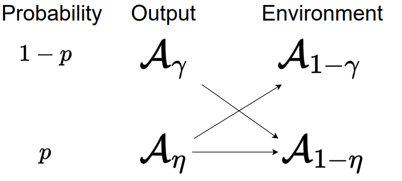
Figure 8: Construction of the degrading map for $p>\frac{1}{2}$, $\eta+\gamma\leq 1$ and $\eta\leq\frac{1}{2}$.

From the picture above, we need probability $p\geq 1-p$ when $\gamma>\frac{1}{2}$, since $\mathcal{A}_{1-\gamma}$ can only be degraded from $\mathcal{A}_{\eta}$ thus probability of $\mathcal{A}_{1-\gamma}$ should be smaller than $\mathcal{A}_{\eta}$. Using this idea, we can characterize the whole region where $\Phi_{p,\gamma,\eta}$ is degradable or anti-degradable.

Proposition IV.1.

$\Phi_{p,\gamma,\eta}$ is degradable if and only if $(p,\gamma,\eta)$ satisfies one of the following conditions:

1. For $p=\frac{1}{2}$: $\eta+\gamma\leq 1$.

2. For $p>\frac{1}{2}$: $\eta+\gamma\leq 1$ and $\eta\leq\frac{1}{2}$.

3. For $p<\frac{1}{2}$: $\eta+\gamma\leq 1$ and $\gamma\leq\frac{1}{2}$.

$\Phi_{p,\gamma,\eta}$ is anti-degradable if and only if $(p,\gamma,\eta)$ satisfies one of the following conditions:

1. For $p=\frac{1}{2}$: $\eta+\gamma\geq 1$.

2. For $p>\frac{1}{2}$: $\eta+\gamma\geq 1$ and $\eta\geq\frac{1}{2}$.

3. For $p<\frac{1}{2}$: $\eta+\gamma\geq 1$ and $\gamma\geq\frac{1}{2}$.

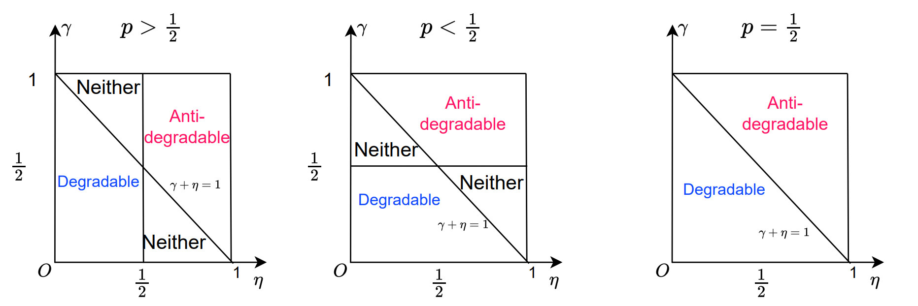
Figure 9: Degradable and anti-degradable regions for $\Phi_{p,\gamma,\eta}$.

Proof.

We only need to prove the degradable case, since by replacing $\gamma$ by $1-\gamma$ and $\eta$ by $1-\eta$, we get the anti-degradable region. Our proof is based on the well-known fact about the inversion and composition of qubit amplitude damping channel [53]: suppose $0\leq\gamma_{1}.\gamma_{2}<1$, the inverse linear map $\mathcal{A}_{\gamma}^{-1}$ is unique and non-positive unless $\gamma=0$. The explicit calculation of the inversion and composition is calculated as

$$\mathcal{A}_{\gamma}^{-1}\begin{pmatrix}\rho_{00}&\rho_{01}\\ \rho_{10}&\rho_{11}\end{pmatrix}=\begin{pmatrix}\rho_{00}-\frac{\gamma}{1-\gamma}\rho_{11}&\frac{1}{\sqrt{1-\gamma}}\rho_{01}\\ \frac{1}{\sqrt{1-\gamma}}\rho_{10}&\frac{1}{1-\gamma}\rho_{11}\end{pmatrix},\quad\mathcal{A}_{\gamma_{2}}\circ\mathcal{A}_{\gamma_{1}}^{-1}\begin{pmatrix}\rho_{00}&\rho_{01}\\ \rho_{10}&\rho_{11}\end{pmatrix}=\begin{pmatrix}\rho_{00}+\frac{\gamma_{2}-\gamma_{1}}{1-\gamma_{1}}\rho_{11}&\frac{\sqrt{1-\gamma_{2}}}{\sqrt{1-\gamma_{1}}}\rho_{01}\\ \frac{\sqrt{1-\gamma_{2}}}{\sqrt{1-\gamma_{1}}}\rho_{10}&\frac{1-\gamma_{2}}{1-\gamma_{1}}\rho_{11}\end{pmatrix}.$$ (87)

In particular, there exists a CPTP map $\mathcal{D}$ such that $\mathcal{D}\circ\mathcal{A}_{\gamma_{1}}=\mathcal{A}_{\gamma_{2}}$ if and only if $\mathcal{A}_{\gamma_{2}}\circ\mathcal{A}_{\gamma_{1}}^{-1}$ is CPTP if and only if $\gamma_{1}\leq\gamma_{2}$. If $\gamma_{1}>\gamma_{2}$, $\mathcal{A}_{\gamma_{2}}\circ\mathcal{A}_{\gamma_{1}}^{-1}$ is non-positive, i.e., there exists $\sigma_{0}\geq 0$ such that $\mathcal{A}_{\gamma_{2}}\circ\mathcal{A}_{\gamma_{1}}^{-1}(\sigma_{0})$ has a negative eigenvalue.

Sufficiency. We prove degradability by explicitly constructing the degrading map depicted in Figure 8. Case 1: $p=\frac{1}{2}$. Since $\gamma+\eta\leq 1$, we have $\gamma\leq 1-\eta$ and $\eta\leq 1-\gamma$ then using (87), there exist qubit degrading maps $\mathcal{D}_{1},\mathcal{D}_{2}$ such that

$$\mathcal{D}_{1}\circ\mathcal{A}_{\gamma}=\mathcal{A}_{1-\eta},\quad\mathcal{D}_{2}\circ\mathcal{A}_{\eta}=\mathcal{A}_{1-\gamma}.$$ (88)

Then using the explicit formula of $(\Phi_{p,\gamma,\eta},\Phi_{p,\gamma,\eta}^{c})$ in (85), it is immediate to see that the degrading map $\mathcal{D}:\mathbb{B}(\mathbb{C}^{2}\otimes\mathbb{C}^{2})\to\mathbb{B}(\mathbb{C}^{2}\otimes\mathbb{C}^{2})$ defined by

$$\mathcal{D}=\mathcal{S}_{10}\otimes\mathcal{D}_{1}+\mathcal{S}_{01}\otimes\mathcal{D}_{2},\quad\mathcal{S}_{ij}(\rho):=\bra{j}\rho\ket{j}\outerproduct{i}{i},\ i,j=0,1$$ (89)

satisfies $\mathcal{D}\circ\Phi_{p,\gamma,\eta}=\Phi_{p,\gamma,\eta}^{c}$. Note that the operational meaning of $\mathcal{S}_{ij}$ is to replace the flag $\ket{j}$ by $\ket{i}$.

Case 2: $1>p>\frac{1}{2}$. Since $\eta\leq\frac{1}{2}$ and $\gamma+\eta\leq 1$, using (87), there exist qubit degrading maps $\mathcal{D}_{1},\mathcal{D}_{2},\mathcal{D}_{3}$ such that

$$\mathcal{D}_{1}\circ\mathcal{A}_{\gamma}=\mathcal{A}_{1-\eta},\quad\mathcal{D}_{2}\circ\mathcal{A}_{\eta}=\mathcal{A}_{1-\eta},\quad\mathcal{D}_{3}\circ\mathcal{A}_{\eta}=\mathcal{A}_{1-\gamma}$$ (90)

Then one can see that the degrading map defined by

$$\mathcal{D}=\mathcal{S}_{10}\otimes\mathcal{D}_{1}+\frac{2p-1}{p}\mathcal{S}_{11}\otimes\mathcal{D}_{2}+\frac{1-p}{p}\mathcal{S}_{01}\otimes\mathcal{D}_{3}$$ (91)

satisfies $\mathcal{D}\circ\Phi_{p,\gamma,\eta}(\rho)=\Phi_{p,\gamma,\eta}(\rho)^{c}$.

Case 3: $0<p<\frac{1}{2}$. Since $\gamma\leq\frac{1}{2}$ and $\gamma+\eta\leq 1$, using (87), there exist qubit degrading maps $\mathcal{D}_{1},\mathcal{D}_{2},\mathcal{D}_{3}$ such that

$$\mathcal{D}_{1}\circ\mathcal{A}_{\gamma}=\mathcal{A}_{1-\eta},\quad\mathcal{D}_{2}\circ\mathcal{A}_{\gamma}=\mathcal{A}_{1-\gamma},\quad\mathcal{D}_{3}\circ\mathcal{A}_{\eta}=\mathcal{A}_{1-\gamma}$$ (92)

Then one can see that the degrading map defined by

$$\mathcal{D}=\frac{p}{1-p}\mathcal{S}_{10}\otimes\mathcal{D}_{1}+\frac{1-2p}{1-p}\mathcal{S}_{00}\otimes\mathcal{D}_{2}+\mathcal{S}_{01}\otimes\mathcal{D}_{3}$$ (93)

satisfies $\mathcal{D}\circ\Phi_{p,\gamma,\eta}(\rho)=\Phi_{p,\gamma,\eta}(\rho)^{c}$.

Sufficiency. The proof follows from proof by contradiction. In fact, we conclude the proof by showing that $\Phi_{p,\gamma,\eta}$ is non-degradable if $(p,\gamma,\eta)$ satisfies one of the following conditions:

1. $\eta+\gamma>1$.

2. $p>\frac{1}{2}$: $\eta+\gamma\leq 1$ and $\eta>\frac{1}{2}$.

3. $p<\frac{1}{2}$: $\eta+\gamma\leq 1$ and $\gamma>\frac{1}{2}$.

Case 1: $\eta+\gamma>1$. Suppose in this case there exists a CPTP degrading map $\mathcal{D}$ such that $\mathcal{D}\circ\Phi_{p,\gamma,\eta}(\rho)=\Phi_{p,\gamma,\eta}(\rho)^{c}$. Then using the Kraus representation of $\mathcal{D}=\sum_{k}E_{k}\cdot E_{k}^{\dagger}$ where $E_{k}=\begin{pmatrix}E_{00}^{k}&E_{01}^{k}\\ E_{10}^{k}&E_{11}^{k}\end{pmatrix},E_{ij}^{k}\in\mathbb{B}(\mathbb{C}^{2})$, we have

$$\sum_{k}\begin{pmatrix}E_{00}^{k}&E_{01}^{k}\\ E_{10}^{k}&E_{11}^{k}\end{pmatrix}\begin{pmatrix}(1-p)\mathcal{A}_{\gamma}&0\\ 0&p\mathcal{A}_{\eta}\end{pmatrix}\begin{pmatrix}(E_{00}^{k})^{\dagger}&(E_{10}^{k})^{\dagger}\\ (E_{01}^{k})^{\dagger}&(E_{11}^{k})^{\dagger}\end{pmatrix}=\begin{pmatrix}(1-p)\mathcal{A}_{1-\gamma}&0\\ 0&p\mathcal{A}_{1-\eta}\end{pmatrix}.$$

Simplifying the above equation, and denote $\mathcal{D}_{ij}=\sum_{k}E_{ij}^{k}\cdot(E_{ij}^{k})^{\dagger}$ we get

$$\begin{cases}(1-p)\mathcal{D}_{00}\circ\mathcal{A}_{\gamma}+p\mathcal{D}_{01}\circ\mathcal{A}_{\eta}=(1-p)\mathcal{A}_{1-\gamma},\\ (1-p)\mathcal{D}_{10}\circ\mathcal{A}_{\gamma}+p\mathcal{D}_{11}\circ\mathcal{A}_{\eta}=p\mathcal{A}_{1-\eta}.\end{cases}$$ (94)

Note that using $\sum_{k}E_{k}^{\dagger}E_{k}=I_{4}$, $\mathcal{D}_{ij}$ are completely positive and trace decreasing such that $\mathcal{D}_{00}+\mathcal{D}_{01}$ and $\mathcal{D}_{10}+\mathcal{D}_{11}$ are quantum channels.

Using the fact that $\mathcal{A}_{1-\gamma}\circ\mathcal{A}_{\eta}^{-1}$ is non-positive via $\eta>1-\gamma$ and similarly $\mathcal{A}_{1-\eta}\circ\mathcal{A}_{\gamma}^{-1}$ is non-positive, (94) is given as

$$\begin{cases}(1-p)\mathcal{D}_{00}\circ\mathcal{A}_{\gamma}\circ\mathcal{A}_{\eta}^{-1}+p\mathcal{D}_{01}=(1-p)\mathcal{A}_{1-\gamma}\circ\mathcal{A}_{\eta}^{-1},\\ (1-p)\mathcal{D}_{10}+p\mathcal{D}_{11}\circ\mathcal{A}_{\eta}\circ\mathcal{A}_{\gamma}^{-1}=p\mathcal{A}_{1-\eta}\circ\mathcal{A}_{\gamma}^{-1}.\end{cases}$$ (95)

On the left hand side, either $\mathcal{A}_{\gamma}\circ\mathcal{A}_{\eta}^{-1}$ or $\mathcal{A}_{\eta}\circ\mathcal{A}_{\gamma}^{-1}$ is completely positive but the right hand side is non-positive and we get a contradiction. Therefore, $\Phi_{p,\gamma,\eta}(\rho)$ is non-degradable.

Case 2: $p>\frac{1}{2}$, $\eta+\gamma\leq 1$ and $\eta>\frac{1}{2}$. In this case, following the same calculation as the previous case, we arrive at (94). We conclude the proof by showing that

$$(1-p)\mathcal{D}_{10}\circ\mathcal{A}_{\gamma}+p\mathcal{D}_{11}\circ\mathcal{A}_{\eta}=p\mathcal{A}_{1-\eta}$$ (96)

is not possible, where $\mathcal{D}_{10}$ and $\mathcal{D}_{11}$ are completely positive and $\mathcal{D}_{10}+\mathcal{D}_{11}$ is trace-preserving. Denote

$$\mathcal{T}_{\mathcal{D}_{10}}=\begin{pmatrix}d_{1}&*&*&d_{3}\\ \cdots&&&\cdots\\ \cdots&&&\cdots\\ d_{2}&*&*&d_{4}\end{pmatrix},\quad\mathcal{T}_{\mathcal{D}_{11}}=\begin{pmatrix}\widetilde{d}_{1}&*&*&\widetilde{d}_{3}\\ \cdots&&&\cdots\\ \cdots&&&\cdots\\ \widetilde{d}_{2}&*&*&\widetilde{d}_{4}\end{pmatrix}.$$

Using the relation between Choi–Jamiołkowski opertor and transfer matrix (25), the Choi–Jamiołkowski opertors $\mathcal{J}_{\mathcal{D}_{10}},\mathcal{J}_{\mathcal{D}_{11}}\geq 0$ are given by

$$\mathcal{J}_{\mathcal{D}_{10}}=\begin{pmatrix}d_{1}&*&*&*\\ *&d_{2}&*&*\\ *&*&d_{3}&*\\ *&*&*&d_{4}\end{pmatrix},\quad\mathcal{J}_{\mathcal{D}_{11}}=\begin{pmatrix}\widetilde{d}_{1}&*&*&*\\ *&\widetilde{d}_{2}&*&*\\ *&*&\widetilde{d}_{3}&*\\ *&*&*&\widetilde{d}_{4}\end{pmatrix}.$$

Also note that $\tr_{2}(\mathcal{J}_{\mathcal{D}_{10}}+\mathcal{J}_{\mathcal{D}_{11}})=I_{2}$, the restriction on $d_{i},\widetilde{d}_{i}$ is given by

$$d_{i},\widetilde{d}_{i}\geq 0,1\leq i\leq 4;\quad d_{1}+\widetilde{d}_{1}+d_{2}+\widetilde{d}_{2}=1;\quad d_{3}+\widetilde{d}_{3}+d_{4}+\widetilde{d}_{4}=1.$$ (97)

Using the composition rule for transfer matrix (24), we have $(1-p)\mathcal{T}_{\mathcal{D}_{10}}\mathcal{T}_{\mathcal{A}_{\gamma}}+p\mathcal{T}_{\mathcal{D}_{11}}\mathcal{T}_{\mathcal{A}_{\eta}}=p\mathcal{T}_{\mathcal{A}_{1-\eta}}$, where the transfer matrix of amplitude damping channel is

$$\mathcal{T}_{\mathcal{A}_{\gamma}}=\begin{pmatrix}1&0&0&\gamma\\ 0&\sqrt{1-\gamma}&0&0\\ 0&0&\sqrt{1-\gamma}&0\\ 0&0&0&1-\gamma\end{pmatrix},$$

and compare the four corner elements, we have

$$\begin{cases}(1-p)d_{1}+p\widetilde{d}_{1}=p,\\ (1-p)d_{2}+p\widetilde{d}_{2}=0,\\ (1-p)[d_{1}\gamma+d_{3}(1-\gamma)]+p[\widetilde{d}_{1}\eta+\widetilde{d}_{3}(1-\eta)]=p(1-\eta),\\ (1-p)[d_{2}\gamma+d_{4}(1-\gamma)]+p[\widetilde{d}_{2}\eta+\widetilde{d}_{4}(1-\eta)]=p\eta.\\ \end{cases}$$

Using the positivity of $d_{i},\widetilde{d}_{i}$, we can conclude by elementary algebra that the only possible solution is $d_{i}=0,1\leq i\leq 4$ thus $\mathcal{D}_{10}=0$. In fact, it is easy to see that $d_{1}=d_{2}=\widetilde{d}_{2}=0,\ \widetilde{d}_{1}=1$. Then the last two equations simplify as

$$(1-p)(1-\gamma)d_{3}+p(1-\eta)\widetilde{d}_{3}=p(1-2\eta),$$

$$(1-p)(1-\gamma)d_{4}+p(1-\eta)\widetilde{d}_{4}=p\eta.$$

Taking the sum, we see that the only possible solution is $d_{3}+d_{4}=0$ thus $\mathcal{D}_{10}=0$. The equation (96) becomes $\mathcal{D}_{11}\circ\mathcal{A}_{\eta}=\mathcal{A}_{1-\eta}$, which is not possible because $\eta>\frac{1}{2}$.

Case 3: $p<\frac{1}{2}$, $\eta+\gamma\leq 1$ and $\gamma>\frac{1}{2}$. This case follows from the same argument as Case 2. In fact, using (94), we can conclude the proof by showing that

$$(1-p)\mathcal{D}_{00}\circ\mathcal{A}_{\gamma}+p\mathcal{D}_{01}\circ\mathcal{A}_{\eta}=(1-p)\mathcal{A}_{1-\gamma}$$

is not possible. Then the same calculation in Case 2 holds if we replace $\eta$ by $\gamma$ and $p$ by $1-p$. ∎

IV.2 Informationally degradable and anti-degradable regions

In the previous subsection, we characterize the regions where the channel $\Phi_{p,\gamma,\eta}$ is neither degradable nor anti-degradable. In this subsection, we provide evidence (rigorous proof for special cases and numerical evidence in full generality) that for any $(\gamma,\eta)$ in that region, there exists a threshold $p^{*}(\gamma,\eta)$ such that when $p$ is above or below the threshold, we have informational degradability or informational anti-degradability introduced in Definition II.1.

To explore the property of informational degradability, we introduce a new quantity called informational advantage of quantum channels:

Definition IV.2.

Given a quantum channel $\mathcal{N}$, the informational advantage of $\mathcal{N}$ at the state $\rho_{VA}$ on the joint system $VA$, is defined as

$$f(\mathcal{N},\rho_{VA})=I(V;B)-I(V;E),$$ (98)

where $I(V;B)=S(B)+S(V)-S(BV)$ is the mutual information of the state $\rho_{VB}=(id_{\mathbb{B}(V)}\otimes\mathcal{N})(\rho_{VA})$.

Using this new quantity, we say that $\mathcal{N}$ is informationally degradable if the informational advantage $f(\mathcal{N},\rho_{VA})$ is non-negative for all quantum system $V$ and quantum state $\rho_{VA}$ on the joint system $VA$. Using the special structure of $\Phi_{p,\gamma,\eta}$, we can simplify the informational advantage:

Lemma IV.3.

The informational advantage of $\Phi_{p,\gamma,\eta}$ is calculated as

$$f(\Phi_{p,\gamma,\eta},\rho_{VA})=(1-p)f(\mathcal{A}_{\gamma},\rho_{VA})+pf(\mathcal{A}_{\eta},\rho_{VA})$$ (99)

for all quantum system $V$ and quantum state $\rho_{VA}$ on the joint system $VA$.

Proof.

The proof follows from the fact that mutual information is additive under convex combination of orthogonal states. ∎

The informational advantage of amplitude damping channels has the following properties:

Lemma IV.4.

The informational advantage of amplitude damping channel $\mathcal{A}_{\gamma}$ satisfies the following

1. $f(\mathcal{A}_{\gamma},\rho_{VA})=0$ if and only if $\rho_{VA}$ is a product state: $\rho_{VA}=\rho_{V}\otimes\rho_{A}$.

2. For any $0<\gamma_{1}<\gamma_{2}<\frac{1}{2}$, we have $0\leq f(\mathcal{A}_{\gamma_{2}},\rho_{VA})\leq f(\mathcal{A}_{\gamma_{1}},\rho_{VA})$.

Proof.

The first property follows from the equality condition of data processing inequality and we show the recovery channel has a unique fixed point, see Appendix A for the details. The second property follows from data processing inequality and the fact that there exists a CPTP map $\mathcal{D}$ such that $\mathcal{D}\circ\mathcal{A}_{\gamma_{1}}=\mathcal{A}_{\gamma_{2}}$ if and only if $\gamma_{1}\leq\gamma_{2}$. ∎

Now back to the region of $(p,\gamma,\eta)$ where $\Phi_{p,\gamma,\eta}$ is neither degradable nor anti-degradable depicted in Figure 9. We focus on the case $p>\frac{1}{2}$ because the other case is similar. When $p>\frac{1}{2}$, if $\gamma+\eta>1$ and $\eta<\frac{1}{2}$, then $\Phi_{p,\gamma,\eta}$ is neither degradable nor anti-degradable. However, since $p$ is the probability of $\mathcal{A}_{\eta}$ which is degradable, as $p$ close to $1$, the channel is dominated by $\mathcal{A}_{\eta}$ and the effect of anti-degradable channel $\mathcal{A}_{\gamma}$ is small. Therefore, $\Phi_{p,\gamma,\eta}$ exhibits some informational advantage. To this end, we study the minimum ratio of informational advantage of amplitude damping channels which indicates multiplicative stability for informational advantage of amplitude damping channels: for any $0<\gamma_{1}<\gamma_{2}<\frac{1}{2}$,

$$R(\gamma_{1},\gamma_{2}):=\inf_{\rho_{VA}}\frac{f(\mathcal{A}_{\gamma_{2}},\rho_{VA})}{f(\mathcal{A}_{\gamma_{1}},\rho_{VA})}.$$ (100)

The infimum should be understood as $\rho_{VA}\neq\rho_{V}\otimes\rho_{A}$ since otherwise, the ratio is $\frac{0}{0}$ by Lemma IV.4. The infimum is obtained when $\rho_{VA}$ is close to its product $\rho_{V}\otimes\rho_{A}$. For similar additive or multiplicative type stability result, we refer to [54, 55, 56, 57, 58]. We have the following conjecture:

Conjecture IV.5.

Multiplicative stability for informational advantage of amplitude damping channels holds:
for any $0<\gamma_{1}<\gamma_{2}<\frac{1}{2}$, $R(\gamma_{1},\gamma_{2})>0$.

We will rigorously show that when the infimum is restricted to pure state, the above conjecture is true. Our key idea is to show for any $\gamma\in(0,\frac{1}{2})$,

$$C(\gamma):=\inf_{\rho_{VA}}\frac{\partial f(\mathcal{A}_{\gamma},\rho_{VA})}{\partial\gamma}/f(\mathcal{A}_{\gamma},\rho_{VA})>-\infty.$$ (101)

Then by taking the logrithmic of $f(\mathcal{A}_{\gamma},\rho_{VA})$ and applying mean-value theorem, for any $0<\gamma_{1}<\gamma_{2}<\frac{1}{2}$, there exists $\xi\in(\gamma_{1},\gamma_{2})$ such that

$$\log(f(\mathcal{A}_{\gamma_{2}},\rho_{VA}))-\log(f(\mathcal{A}_{\gamma_{1}},\rho_{VA}))=\left(\frac{\partial f(\mathcal{A}_{\xi},\rho_{VA})}{\partial\gamma}/f(\mathcal{A}_{\xi},\rho_{VA})\right)(\gamma_{2}-\gamma_{1})\geq\inf_{\xi\in[\gamma_{1},\gamma_{2}]}C(\xi)(\gamma_{2}-\gamma_{1}).$$ (102)

Then taking exponential on both sides, we get the desired result. Our analysis shows that by taking the infimum over pure states, $C(\gamma)$ is finite for all $\gamma\in(0,\frac{1}{2})$ and $C(\gamma)\to-\infty$ if $\gamma$ tends to $0$ or $\frac{1}{2}$ therefore $R(\gamma_{1},\gamma_{2})$ will tend to zero if $\gamma_{i}$ tends to $0$ or $\frac{1}{2}$. This feature is captured in our numerical evaluation. Moreover, in full generality, our numerical evidence is that the infimum will not decrease if the dimension of $V$ is higher than $2$ and $R(\gamma_{1},\gamma_{2})$ with $\text{dim}V=2$ is depicted in Figure 5.

Proposition IV.6.

If Conjecture IV.5 is true, then in the region where $\Phi_{p,\gamma,\eta}$ is neither degradable nor anti-degradable, we have

• For any $(\gamma,\eta)$ such that $\gamma+\eta>1$ and $\eta<\frac{1}{2}$, there exists a threshold $p^{*}(\gamma,\eta)\in(\frac{1}{2},1)$ such that when $p\geq p^{*}(\gamma,\eta)$, $\Phi_{p,\gamma,\eta}$ is informationally degradable.

• For any $(\gamma,\eta)$ such that $\gamma+\eta<1$ and $\eta>\frac{1}{2}$, there exists a threshold $p^{*}(\gamma,\eta)\in(\frac{1}{2},1)$ such that when $p\geq p^{*}(\gamma,\eta)$, $\Phi_{p,\gamma,\eta}$ is informationally anti-degradable.

• For any $(\gamma,\eta)$ such that $\gamma+\eta>1$ and $\gamma<\frac{1}{2}$, there exists a threshold $p^{*}(\gamma,\eta)\in(0,\frac{1}{2})$ such that when $p\leq p^{*}(\gamma,\eta)$, $\Phi_{p,\gamma,\eta}$ is informationally degradable.

• For any $(\gamma,\eta)$ such that $\gamma+\eta<1$ and $\gamma>\frac{1}{2}$, there exists a threshold $p^{*}(\gamma,\eta)\in(0,\frac{1}{2})$ such that when $p\leq p^{*}(\gamma,\eta)$, $\Phi_{p,\gamma,\eta}$ is informationally anti-degradable.

Proof.

We only show the first argument since the others are similar. For $\gamma+\eta>1$ and $\eta<\frac{1}{2}$, by Lemma IV.3, the informational advantage of $\Phi_{p,\gamma,\eta}$ is calculated as

$$f(\Phi_{p,\gamma,\eta},\rho_{VA}) =(1-p)f(\mathcal{A}_{\gamma},\rho_{VA})+pf(\mathcal{A}_{\eta},\rho_{VA})$$

$$=pf(\mathcal{A}_{\eta},\rho_{VA})-(1-p)f(\mathcal{A}_{1-\gamma},\rho_{VA})\geq 0\iff p\geq\frac{1}{1+\frac{f(\mathcal{A}_{\eta},\rho_{VA})}{f(\mathcal{A}_{1-\gamma},\rho_{VA})}}$$

Note that $0<1-\gamma<\eta<\frac{1}{2}$, by Conjecture IV.5 we have $\inf_{\rho_{VA}}\frac{f(\mathcal{A}_{\eta},\rho_{VA})}{f(\mathcal{A}_{1-\gamma},\rho_{VA})}>0$ thus choose $p^{*}(\gamma,\eta):=\frac{1}{1+\inf_{\rho_{VA}}\frac{f(\mathcal{A}_{\eta},\rho_{VA})}{f(\mathcal{A}_{1-\gamma},\rho_{VA})}}\in(\frac{1}{2},1)$ we conclude the proof. ∎

Appendix A Proof of Lemma IV.4

In this section, we aim to prove the first part of Lemma IV.4. Using the definition of informational advantage, it is equivalent to show that for $\gamma<\frac{1}{2}$, any quantum system $V$ and quantum state $\rho_{VA}$,

$$I(V;B)=I(V;E)$$ (103)

if and only if $\rho_{VA}=\rho_{V}\otimes\rho_{A}$. Recall that $\mathcal{A}_{\gamma}$ is degradable and the composition rule is given as

$$I(V;B)=D(\rho_{VB}\|\rho_{V}\otimes\rho_{B}),$$

$$I(V;E)=D((I_{V}\otimes\mathcal{A}_{\frac{1-2\gamma}{1-\gamma}})(\rho_{VB})\|(I_{V}\otimes\mathcal{A}_{\frac{1-2\gamma}{1-\gamma}})(\rho_{V}\otimes\rho_{B})).$$

Therefore, by data processing inequality, one has $I(V;B)\geq I(V;E)$. Recall that the equality condition for data processing inequality, we have $I(V;B)=I(V;E)$ if and only if [34, 59, 60]

$$\mathcal{R}_{I_{V}\otimes\mathcal{A}_{\frac{1-2\gamma}{1-\gamma}},\rho_{V}\otimes\rho_{B}}((I_{V}\otimes\mathcal{A}_{\frac{1-2\gamma}{1-\gamma}})(\rho_{VB}))=\rho_{VB},$$ (104)

where the recovery map $\mathcal{R}_{\mathcal{N},\sigma}$ for given quantum channel $\mathcal{N}$ and quantum state $\sigma$ is defined by

$$\mathcal{R}_{\mathcal{N},\sigma}(X):=\sigma^{1/2}\mathcal{N}^{*}\big{(}\mathcal{N}(\sigma)^{-1/2}\mathcal{N}(X)\mathcal{N}(\sigma)^{-1/2}\big{)}\sigma^{1/2},\quad\text{supp}(X)\subseteq\text{supp}(\mathcal{N}(\sigma)).$$ (105)

Now denote $\gamma^{\prime}=\frac{1-2\gamma}{1-\gamma}$ and use the Kraus representation for $\mathcal{A}_{\gamma^{\prime}}(\rho):=\sum_{i=0}^{1}E_{i}\rho E_{i}^{\dagger}$, with

$$E_{0}=\begin{pmatrix}1&0\\ 0&\sqrt{1-\gamma^{\prime}}\end{pmatrix},E_{1}=\begin{pmatrix}0&\sqrt{\gamma^{\prime}}\\ 0&0\end{pmatrix},$$ (106)

we can write the Kraus representation of the channel $\mathcal{R}_{I_{V}\otimes\mathcal{A}_{\gamma^{\prime}},\rho_{V}\otimes\rho_{B}}\circ(I_{V}\otimes\mathcal{A}_{\gamma^{\prime}})$ as

$$\mathcal{R}_{I_{V}\otimes\mathcal{A}_{\gamma^{\prime}},\rho_{V}\otimes\rho_{B}}\circ(I_{V}\otimes\mathcal{A}_{\gamma^{\prime}})(X)=\sum_{i,j}(I_{V}\otimes A_{ij})X(I_{V}\otimes A_{ij})^{\dagger},\quad X\in\mathbb{B}(V\otimes B),$$ (107)

where

$$A_{ij}=\rho_{B}^{1/2}E_{i}^{\dagger}\mathcal{A}_{\gamma^{\prime}}(\rho_{B})^{-1/2}E_{j},i,j=0,1.$$ (108)

Denote the quantum channel with Kraus operator $\{A_{ij}\}$ by

$$\mathcal{N}(\rho):=\sum_{i,j}A_{ij}\rho A_{ij}^{\dagger}.$$ (109)

Then (104) becomes

$$I_{V}\otimes\mathcal{N}(\rho_{VB})=\rho_{VB}.$$ (110)

The following proposition characterizes the fixed point algebra of $I_{V}\otimes\mathcal{N}$ when $\mathcal{N}$ has a unique fixed point.

Proposition A.1.

Suppose $\mathcal{N}$ has a unique fixed state, i.e., there exists a unique quantum state $\rho_{0}$, such that $\mathcal{N}(\rho_{0})=\rho_{0}$, then for any finite dimensional quantum system $V$, and quantum state $\rho_{VB}$,

$$I_{V}\otimes\mathcal{N}(\rho_{VB})=\rho_{VB}$$ (111)

implies $\rho_{VB}=\rho_{V}\otimes\rho_{B}$ and $\rho_{B}=\rho_{0}$.

Proof.

Suppose $\{\ket{i}_{V}\}_{0\leq i\leq n-1}$ is a standard basis of $V$ and decompose $\rho_{VB}$ as

$$\rho_{VB}=\sum_{i,j}\ket{i}\bra{j}_{V}\otimes\rho_{B}^{ij}.$$ (112)

For any $0\leq k\leq n-1$, using (111), we know that

$$\bra{k}_{V}(I_{V}\otimes\mathcal{N}(\rho_{VB}))\ket{k}_{V}=\bra{k}_{V}\rho_{VB}\ket{k}_{V}=\mathcal{N}(\rho_{B}^{kk})=\rho_{B}^{kk}\geq 0.$$ (113)

Therefore, if $\Tr(\rho_{B}^{kk})\neq 0$, $\frac{\rho_{B}^{kk}}{\Tr(\rho_{B}^{kk})}$ is a fixed point of $\mathcal{N}$ thus equal to $\rho_{0}$. If $\Tr(\rho_{B}^{kk})=0$, then we have $\rho_{B}^{kk}=0=0\cdot\rho_{0}$. In summary, one has

$$\rho_{B}^{kk}=\Tr(\rho_{B}^{kk})\rho_{0}.$$ (114)

For any $0\leq k<l\leq n-1$, define $\ket{\psi}=\alpha\ket{k}_{V}+\beta\ket{l}_{V}$, with $\alpha,\beta\in\mathbb{C},|\alpha|^{2}+|\beta|^{2}=1$. Using (111), we know that

$$\bra{\psi}(I_{V}\otimes\mathcal{N}(\rho_{VB}))\ket{\psi}=\bra{\psi}\rho_{VB}\ket{\psi}$$ (115)

$$=\mathcal{N}(|\alpha|^{2}\rho_{B}^{kk}+\bar{\alpha}\beta\rho_{B}^{kl}+\bar{\beta}\alpha\rho_{B}^{lk}+|\beta|^{2}\rho_{B}^{ll})=|\alpha|^{2}\rho_{B}^{kk}+\bar{\alpha}\beta\rho_{B}^{kl}+\bar{\beta}\alpha\rho_{B}^{lk}+|\beta|^{2}\rho_{B}^{ll}.$$

Using the same argument as before, one has

$$|\alpha|^{2}\rho_{B}^{kk}+\bar{\alpha}\beta\rho_{B}^{kl}+\bar{\beta}\alpha\rho_{B}^{lk}+|\beta|^{2}\rho_{B}^{ll}=\Tr\big(|\alpha|^{2}\rho_{B}^{kk}+\bar{\alpha}\beta\rho_{B}^{kl}+\bar{\beta}\alpha\rho_{B}^{lk}+|\beta|^{2}\rho_{B}^{ll}\big{missing})\rho_{0}.$$

Recall the diagonal terms are proportional to $\rho_{0}$ (114), one has

$$\bar{\alpha}\beta\rho_{B}^{kl}+\bar{\beta}\alpha\rho_{B}^{lk}=\Tr\big(\bar{\alpha}\beta\rho_{B}^{kl}+\bar{\beta}\alpha\rho_{B}^{lk}\big{missing})\rho_{0}.$$ (116)

Since the choice of $\alpha,\beta$ in $\ket{\psi}=\alpha\ket{k}_{V}+\beta\ket{l}_{V}$ is arbitrary as long as $|\alpha|^{2}+|\beta|^{2}=1$, by $|\bar{\alpha}\beta|\leq\frac{|\alpha|^{2}+|\beta|^{2}}{2}$, the range of $\bar{\alpha}\beta$ is given by

$$\{c\in\mathbb{C}:|c|\leq\frac{1}{2}\}.$$ (117)

Therefore, note that $\rho_{VB}$ is self-adjoint, we have $\rho_{B}^{kl}=(\rho_{B}^{lk})^{\dagger}$, (116) is equivalent to

$$\forall c\in\mathbb{C},|c|\leq\frac{1}{2},\quad c\rho_{B}^{kl}+(c\rho_{B}^{kl})^{\dagger}=\Tr(c\rho_{B}^{kl}+(c\rho_{B}^{kl})^{\dagger})\rho_{0},$$ (118)

which implies

$$\rho_{B}^{kl}=\Tr(\rho_{B}^{kl})\rho_{0}.$$

In fact, denote

$$\rho_{B}^{kl}=(x_{uv})_{0\leq u,v\leq\text{dim}B-1},\rho_{0}=(\rho_{uv})_{0\leq u,v\leq\text{dim}B-1}.$$

Compare each element in the above equation, for any $0\leq u,v\leq\text{dim}B-1$,

$$c(x_{uv}-\rho_{uv}\sum_{r}x_{rr})+\overline{c}(\overline{x_{uv}}-\overline{\rho_{uv}\sum_{r}x_{rr}})=0.$$

Since $|c|\leq\frac{1}{2}$ can be any complex number, we must have

$$x_{uv}=\rho_{uv}\sum_{r}x_{rr},$$ (119)

which means $\rho_{B}^{kl}=\Tr(\rho_{B}^{kl})\rho_{0}$. In summary, by showing that for any $0\leq k,l\leq n-1$, $\rho_{B}^{kl}=\Tr(\rho_{B}^{kl})\rho_{0}$, we arrive at the conclusion

$$\rho_{VB}=\sum_{i,j}\ket{i}\bra{j}_{V}\otimes\rho_{B}^{i,j}=\sum_{i,j}\Tr(\rho_{B}^{ij})\ket{i}\bra{j}_{V}\otimes\rho_{0}=\rho_{V}\otimes\rho_{0}.$$ (120)

∎

Remark A.2.

(This discussion is due to Mohammad A. Alhejji) Note that if $\mathcal{N}$ has multiple fixed states $\rho_{0}\neq\rho_{1}$, then there exists a non-product state $\widetilde{\rho}_{VB}$ given by

$$\widetilde{\rho}_{VB}=\frac{1}{2}\outerproduct{0}{0}_{V}\otimes\rho_{0}+\frac{1}{2}\outerproduct{1}{1}_{V}\otimes\rho_{1},$$ (121)

such that $I_{V}\otimes\mathcal{N}(\widetilde{\rho}_{VB})=\widetilde{\rho}_{VB}$.

The remaining task is to show the quantum channel defined by (109) has a unique fixed point. What we need is the following proposition, proved in [61, Proposition 6.8]:

Proposition A.3.

Suppose $\mathcal{N}:\mathbb{B}(\mathcal{H})\to\mathbb{B}(\mathcal{H})$ is a (non-unital) quantum channel. If the Kraus representation of $\mathcal{N}$ given by

$$\mathcal{N}(\rho):=\sum_{i\in I}E_{i}\rho E_{i}^{\dagger}$$ (122)

satisfies: $\exists n\geq 1,\text{span}\{\prod_{k\leq n}E_{i_{k}}:i_{k}\in I\}=\mathbb{B}(\mathcal{H})$. Then $\mathcal{N}$ has a unique fixed point.

Proof of Lemma IV.4: Using Proposition A.1, we only need to show the recovery channel $\mathcal{N}$ defined in (109) $\mathcal{N}(\rho):=\sum_{i,j}A_{ij}\rho A_{ij}^{\dagger}$ where $A_{ij}=\rho_{B}^{1/2}E_{i}^{\dagger}\mathcal{A}_{\gamma^{\prime}}(\rho_{B})^{-1/2}E_{j},i,j=0,1$ has a unique fixed point.

Case 1: If $\rho_{B}=\outerproduct{0}{0}$, we have $\mathcal{A}_{\gamma^{\prime}}(\rho_{B})=\outerproduct{0}{0}$. Therefore, the support of the recovery map is spanned by single vector $\ket{0}$ and it is trivial(identity). Therefore, in this case the equality condition is given by

$$\rho_{VB}=I_{V}\otimes\mathcal{A}_{\gamma^{\prime}}(\rho_{VB}).$$ (123)

Note that $\mathcal{A}_{\gamma^{\prime}}$ has a unique fixed point $\outerproduct{0}{0}$ thus $\rho_{VB}=\rho_{V}\otimes\outerproduct{0}{0}$.

Case 2: If $\rho_{B}=\begin{pmatrix}1-p&\delta\\ \delta^{*}&p\end{pmatrix}$ for $p\in(0,1)$, then denote

$$\Delta_{1}:=p(1-p)-|\delta|^{2},$$

$$\Delta_{2}:=(1-\gamma^{\prime})\Delta_{1}+\gamma^{\prime}(1-\gamma^{\prime})p^{2},$$

$$\Delta:=\frac{1}{\sqrt{\Delta_{2}(1+2\sqrt{\Delta_{1}})(1+2\sqrt{\Delta_{2}})}}.$$

We have

$$A_{00}/\Delta=$$

$$\begin{pmatrix}(1-\gamma^{\prime})\sqrt{\Delta_{1}}(\sqrt{\Delta_{1}}+p)+\sqrt{\Delta_{2}}(1-p+\sqrt{\Delta_{1}})&\delta(1-\gamma^{\prime})(\gamma^{\prime}p+\sqrt{\Delta_{2}}-\sqrt{\Delta_{1}}))\\ (\sqrt{\Delta_{2}}-(1-\gamma^{\prime})\sqrt{\Delta_{1}})\delta^{*}&(1-\gamma^{\prime})(\Delta_{1}+(p+\sqrt{\Delta_{1}})(\gamma^{\prime}p+\sqrt{\Delta_{2}}+(1-p)\sqrt{\Delta_{1}}\end{pmatrix}$$

$$A_{01}=\Delta\begin{pmatrix}0&\sqrt{\gamma^{\prime}}\big{(}(1-\gamma^{\prime})(\Delta_{1}+p\sqrt{\Delta_{1}})+\sqrt{\Delta_{2}}(\sqrt{\Delta_{1}}+1-p)\big{)}\\ 0&\sqrt{\gamma^{\prime}}\delta^{*}(\sqrt{\Delta_{2}}-(1-\gamma^{\prime})\sqrt{\Delta_{1}})\end{pmatrix}$$

$$A_{10}=\Delta\begin{pmatrix}\delta\sqrt{\gamma^{\prime}}(\sqrt{\Delta_{2}}+(1-\gamma^{\prime})p)&\sqrt{\gamma^{\prime}}(1-\gamma^{\prime})\delta^{2}\\ \sqrt{\gamma^{\prime}}(\sqrt{\Delta_{1}}+p)(\sqrt{\Delta_{2}}+(1-\gamma^{\prime})p)&-\delta\sqrt{\gamma^{\prime}}(1-\gamma^{\prime})(\sqrt{\Delta_{1}}+p)\end{pmatrix}$$

$$A_{11}=\Delta\begin{pmatrix}0&\delta\gamma^{\prime}(\sqrt{\Delta_{2}}+(1-\gamma^{\prime})p)\\ 0&\gamma^{\prime}(\sqrt{\Delta_{2}}+(1-\gamma^{\prime})p)(p+\sqrt{\Delta_{1}}).\end{pmatrix}$$

One can directly check that

$$\text{span}\{A_{ij}\}=\mathbb{M}_{2},$$ (124)

thus using Proposition A.3 we conclude the proof. ∎

Appendix B Proof of Conjecture IV.5 in special cases

Following the argument after (101), our goal is to show that

$$C(\gamma):=\inf_{\rho_{VA}}\frac{\partial f(\mathcal{A}_{\gamma},\rho_{VA})}{\partial\gamma}/f(\mathcal{A}_{\gamma},\rho_{VA})>-\infty.$$

In this section, we prove that

$$\inf_{\ket{\psi}_{VA}}\frac{\partial f(\mathcal{A}_{\gamma},\outerproduct{\psi}{\psi}_{VA})}{\partial\gamma}/f(\mathcal{A}_{\gamma},\outerproduct{\psi}{\psi}_{VA})>-\infty$$ (125)

and leave the more general case as an open question. In the case $\rho_{VA}=\outerproduct{\psi}{\psi}_{VA}$, we define a simpler version of advantange, which is given by

$$f(\gamma,\rho_{A})=S(\mathcal{A}_{\gamma}(\rho_{A}))-S(\mathcal{A}_{\gamma}^{c}(\rho_{A})).$$ (126)

Note that the above advantage function is half of $f(\mathcal{A}_{\gamma},\rho_{VA})$ with the restriction of $\rho_{VA}$ to be a pure state. In fact, since $\rho_{VA}$ is pure, then $\rho_{VBE}$ is pure thus

$$f(\mathcal{A}_{\gamma},\rho_{VA})=I(V;B)-I(V;E)=S(B)-S(E)-(S(BV)-S(EV))=2(S(B)-S(E)).$$ (127)

Then we can show the following lemma:

Lemma B.1.

For any $\gamma\in(0,\frac{1}{2})$,

$$\inf_{\rho_{A}}\frac{\frac{\partial f}{\partial\gamma}(\gamma,\rho_{A})}{f(\gamma,\rho_{A})}=A(\gamma)>-\infty.$$ (128)

Proof.

Suppose the initial state $\rho_{A}=\begin{pmatrix}1-p&\delta\\ \delta^{*}&p\end{pmatrix}$ with $|\delta|^{2}\leq p(1-p)$. Then $\rho_{B}=\begin{pmatrix}1-(1-\gamma)p&\sqrt{1-\gamma}\delta\\ \sqrt{1-\gamma}\delta^{*}&(1-\gamma)p\end{pmatrix}$. By direct calculation, the eigenvalue of $\rho_{B}$ is given by

$$\frac{1+\sqrt{4(1-\gamma)|\delta|^{2}+(2(1-\gamma)p-1)^{2}}}{2},\frac{1-\sqrt{4(1-\gamma)|\delta|^{2}-(2(1-\gamma)p-1)^{2}}}{2}$$ (129)

thus denote $h_{2}(x):=-x\log x-(1-x)\log(1-x)$ we have

$$S(B)=h_{2}(\frac{1+\sqrt{4(1-\gamma)|\delta|^{2}+(2(1-\gamma)p-1)^{2}}}{2}).$$

Similarly, we have

$$S(E)=h_{2}(\frac{1+\sqrt{4\gamma|\delta|^{2}+(2\gamma p-1)^{2}}}{2}).$$

Denote $t:=|\delta|^{2}$, then we need to show that the function defined by

$$f(\gamma,p,t):=h_{2}(\frac{1+\sqrt{4(1-\gamma)t+(2(1-\gamma)p-1)^{2}}}{2})-h_{2}(\frac{1+\sqrt{4\gamma t+(2\gamma p-1)^{2}}}{2})$$ (130)

satisfies

$$\inf_{p\in[0,1],t\in[0,p(1-p)]}\frac{\frac{\partial f}{\partial\gamma}(\gamma,p,t)}{f(\gamma,p,t)}=A(\gamma)>-\infty.$$ (131)

Denote the function

$$g(\gamma,p,t)=\frac{1+\sqrt{(1-2\gamma p)^{2}+4\gamma t}}{2},$$ (132)

and we have

$$\frac{\partial g}{\partial\gamma}(\gamma,p,t)=\frac{-p(1-2\gamma p)+t}{\sqrt{(1-2\gamma p)^{2}+4\gamma t}}.$$ (133)

Then we rewrite the function $f(\gamma,p,t)=h_{2}(g(1-\gamma,p,t))-h_{2}(g(\gamma,p,t))$ and using chain rule and the fact that $h_{2}^{\prime}(x)=\log(1-x)-\log x$, we have

$$\frac{\partial f}{\partial\gamma}(\gamma,p,t) =-h_{2}^{\prime}(g(1-\gamma,p,t))\frac{\partial g}{\partial\gamma}(1-\gamma,p,t)-h_{2}^{\prime}(g(\gamma,p,t))\frac{\partial g}{\partial\gamma}(\gamma,p,t)$$ (134)

$$=-\frac{-p(1-2(1-\gamma)p)+t}{\sqrt{(1-2(1-\gamma)p)^{2}+4(1-\gamma)t}}\big{(}\log(1-g(1-\gamma,p,t))-\log(g(1-\gamma,p,t))\big{)}$$

$$-\frac{-p(1-2\gamma p)+t}{\sqrt{(1-2\gamma p)^{2}+4\gamma t}}\big{(}\log(1-g(\gamma,p,t))-\log(g(\gamma,p,t))\big{)}.$$

First we note that

$$f(\gamma,p,t)=0\iff p(1-p)-t=0$$ (135)

In fact,

$$g(1-\gamma,p,t)-g(\gamma,p,t) =\frac{1}{2}(\sqrt{(1-2(1-\gamma)p)^{2}+4(1-\gamma)t}-\sqrt{(1-2\gamma p)^{2}+4\gamma t})$$

$$=\frac{1}{2}\frac{(1-2(1-\gamma)p)^{2}+4(1-\gamma)t-(1-2\gamma p)^{2}-4\gamma t}{\sqrt{(1-2(1-\gamma)p)^{2}+4(1-\gamma)t}+\sqrt{(1-2\gamma p)^{2}+4\gamma t}}$$

$$=\frac{-2(1-2\gamma)(p(1-p)-t)}{\sqrt{(1-2(1-\gamma)p)^{2}+4(1-\gamma)t}+\sqrt{(1-2\gamma p)^{2}+4\gamma t}}$$

$$\leq 0,$$

and note that $g(1-\gamma,p,t),g(\gamma,p,t)\in[\frac{1}{2},1]$, $h_{2}(x)$ is decreasing on $[\frac{1}{2},1]$ thus we have $f(\gamma,p,t)\geq 0$ and $f(\gamma,p,t)=0\iff p(1-p)-t=0$.

Moreover, if $p(1-p)-t=0$, we have $g(1-\gamma,p,t)=g(\gamma,p,t)$ thus $(1-2(1-\gamma)p)^{2}+4(1-\gamma)t=(1-2\gamma p)^{2}+4\gamma t$, and $\frac{\partial f}{\partial\gamma}(\gamma,p,t)=0.$

We then need to show that when $t\to p(1-p)$

$$\lim_{t\to p(1-p)}\frac{\frac{\partial f}{\partial\gamma}(\gamma,p,t)}{f(\gamma,p,t)},$$ (136)

converges to a uniformly bounded function of $p$.

The tasks are calculating

$$\frac{\partial^{2}f}{\partial\gamma\partial t}(\gamma,p,t),\frac{\partial f}{\partial t}(\gamma,p,t)$$ (137)

and use Taylor expansion to get

$$\lim_{t\to p(1-p)}\frac{\frac{\partial f}{\partial\gamma}(\gamma,p,t)}{f(\gamma,p,t)}=\frac{\frac{\partial^{2}f}{\partial\gamma\partial t}(\gamma,p,t)}{\frac{\partial f}{\partial t}(\gamma,p,t)}\bigg{|}_{t=p(1-p)}.$$ (138)

To calculate $\frac{\partial^{2}f}{\partial\gamma\partial t}(\gamma,p,t)$, denote a function $w(\gamma,p,t)$ by

$$w(\gamma,p,t)=-\frac{-p(1-2\gamma p)+t}{\sqrt{(1-2\gamma p)^{2}+4\gamma t}}\big{(}\log(1-g(\gamma,p,t))-\log(g(\gamma,p,t))\big{)}.$$ (139)

Then by (134), we have

$$\frac{\partial f}{\partial\gamma}(\gamma,p,t)=w(\gamma,p,t)+w(1-\gamma,p,t).$$ (140)

Using the chain rule, we have

$$\frac{\partial w}{\partial t}(\gamma,p,t) =-\frac{\partial}{\partial t}\big{(}\frac{-p(1-2\gamma p)+t}{\sqrt{(1-2\gamma p)^{2}+4\gamma t}}\big{)}\big{(}\log(1-g(\gamma,p,t))-\log(g(\gamma,p,t))\big{)}$$

$$-\frac{-p(1-2\gamma p)+t}{\sqrt{(1-2\gamma p)^{2}+4\gamma t}}\frac{\partial}{\partial t}\big{(}\log(1-g(\gamma,p,t))-\log(g(\gamma,p,t))\big{)}$$

$$=-\frac{1-2\gamma p+2\gamma t}{((1-2\gamma p)^{2}+4\gamma t)^{\frac{3}{2}}}\big{(}\log(1-g(\gamma,p,t))-\log(g(\gamma,p,t))\big{)}$$

$$-\frac{-p(1-2\gamma p)+t}{\sqrt{(1-2\gamma p)^{2}+4\gamma t}}\bigg{(}-\frac{1}{(p(1-p)-t+(1-\gamma)p^{2})\sqrt{(1-2\gamma p)^{2}+4\gamma t}}\bigg{)}$$

$$=-\frac{1-2\gamma p+2\gamma t}{((1-2\gamma p)^{2}+4\gamma t)^{\frac{3}{2}}}\big{(}\log(1-g(\gamma,p,t))-\log(g(\gamma,p,t))\big{)}$$

$$+\frac{1}{(1-2\gamma p)^{2}+4\gamma t}\frac{-p(1-p)+t-(1-2\gamma)p^{2}}{p(1-p)-t+(1-\gamma)p^{2}}$$

Then

$$\frac{\partial^{2}f}{\partial\gamma\partial t}(\gamma,p,t) =\frac{\partial w}{\partial t}(\gamma,p,t)+\frac{\partial w}{\partial t}(1-\gamma,p,t)$$

$$=-\frac{1-2\gamma p+2\gamma t}{((1-2\gamma p)^{2}+4\gamma t)^{\frac{3}{2}}}\big{(}\log(1-g(\gamma,p,t))-\log(g(\gamma,p,t))\big{)}$$

$$+\frac{1}{(1-2\gamma p)^{2}+4\gamma t}\frac{-p(1-p)+t-(1-2\gamma)p^{2}}{p(1-p)-t+(1-\gamma)p^{2}}$$

$$-\frac{1-2(1-\gamma)p+2(1-\gamma)t}{((1-2(1-\gamma)p)^{2}+4(1-\gamma)t)^{\frac{3}{2}}}\big{(}\log(1-g(1-\gamma,p,t))-\log(g(1-\gamma,p,t))\big{)}$$

$$+\frac{1}{(1-2(1-\gamma)p)^{2}+4(1-\gamma)t}\frac{-p(1-p)+t-(1-2(1-\gamma))p^{2}}{p(1-p)-t+\gamma p^{2}}.$$

We plug $t=p(1-p)$ into the above equation. Note that when $t=p(1-p)$, we have

$$(1-2\gamma p)^{2}+4\gamma t=(1-2(1-\gamma)p)^{2}+4(1-\gamma)t=1-4\gamma(1-\gamma)p^{2}$$ (141)

thus

$$\frac{\partial^{2}f}{\partial\gamma\partial t}(\gamma,p,t)\bigg{|}_{t=p(1-p)}=\frac{\partial w}{\partial t}(\gamma,p,t)\bigg{|}_{t=p(1-p)}+\frac{\partial w}{\partial t}(1-\gamma,p,t)\bigg{|}_{t=p(1-p)}$$ (142)

$$=-\frac{1-2\gamma p^{2}}{(1-4\gamma(1-\gamma)p^{2})^{\frac{3}{2}}}\log(\frac{1-\sqrt{1-4\gamma(1-\gamma)p^{2}}}{1+\sqrt{1-4\gamma(1-\gamma)p^{2}}})-\frac{1}{1-4\gamma(1-\gamma)p^{2}}\frac{1-2\gamma}{1-\gamma}$$

$$-\frac{1-2(1-\gamma)p^{2}}{(1-4\gamma(1-\gamma)p^{2})^{\frac{3}{2}}}\log(\frac{1-\sqrt{1-4\gamma(1-\gamma)p^{2}}}{1+\sqrt{1-4\gamma(1-\gamma)p^{2}}})-\frac{1}{1-4\gamma(1-\gamma)p^{2}}\frac{2\gamma-1}{\gamma}$$

$$=-\frac{2-2p^{2}}{(1-4\gamma(1-\gamma)p^{2})^{\frac{3}{2}}}\log(\frac{1-\sqrt{1-4\gamma(1-\gamma)p^{2}}}{1+\sqrt{1-4\gamma(1-\gamma)p^{2}}})+\frac{(1-2\gamma)^{2}}{\gamma(1-\gamma)}\frac{1}{1-4\gamma(1-\gamma)p^{2}}$$

The calculation of $\frac{\partial f}{\partial t}(\gamma,p,t)$ proceeds as follows:

$$\frac{\partial f}{\partial t}(\gamma,p,t) =h_{2}^{\prime}(g(1-\gamma,p,t))\frac{\partial g}{\partial t}(1-\gamma,p,t)-h_{2}^{\prime}(g(\gamma,p,t))\frac{\partial g}{\partial t}(\gamma,p,t)$$

$$=\frac{1-\gamma}{\sqrt{(1-2(1-\gamma)p)^{2}+4(1-\gamma)t}}\big{(}\log(1-g(1-\gamma,p,t))-\log(g(1-\gamma,p,t))\big{)}$$

$$-\frac{\gamma}{\sqrt{(1-2\gamma p)^{2}+4\gamma t}}\big{(}\log(1-g(\gamma,p,t))-\log(g(\gamma,p,t))\big{)}.$$

Similar as before, we plug $t=p(1-p)$ into the above formula, thus

$$\frac{\partial f}{\partial t}(\gamma,p,t)\bigg{|}_{t=p(1-p)}=\frac{1-2\gamma}{\sqrt{1-4\gamma(1-\gamma)p^{2}}}\log(\frac{1-\sqrt{1-4\gamma(1-\gamma)p^{2}}}{1+\sqrt{1-4\gamma(1-\gamma)p^{2}}})$$ (143)

Combine the calculation of $\frac{\partial^{2}f}{\partial\gamma\partial t}(\gamma,p,t)\bigg{|}_{t=p(1-p)}$ in (142) and $\frac{\partial f}{\partial t}(\gamma,p,t)\bigg{|}_{t=p(1-p)}$ in (143), and note that $(1-2\gamma)^{2}\leq 1-4\gamma(1-\gamma)p^{2}\leq 1$ we have

$$\lim_{t\to p(1-p)}\frac{\frac{\partial f}{\partial\gamma}(\gamma,p,t)}{f(\gamma,p,t)}=\frac{\frac{\partial^{2}f}{\partial\gamma\partial t}(\gamma,p,t)}{\frac{\partial f}{\partial t}(\gamma,p,t)}\bigg{|}_{t=p(1-p)}$$

$$=-\frac{2-2p^{2}}{(1-4\gamma(1-\gamma)p^{2})(1-2\gamma)}+\frac{1-2\gamma}{\gamma(1-\gamma)\sqrt{1-4\gamma(1-\gamma)p^{2}}\log(\frac{1-\sqrt{1-4\gamma(1-\gamma)p^{2}}}{1+\sqrt{1-4\gamma(1-\gamma)p^{2}}})}$$

$$\geq-\frac{2-2p^{2}}{(1-2\gamma)^{3}}+\frac{1}{\gamma(1-\gamma)\log(\frac{1-\sqrt{1-4\gamma(1-\gamma)p^{2}}}{1+\sqrt{1-4\gamma(1-\gamma)p^{2}}})}$$

$$\geq-\frac{2}{(1-2\gamma)^{3}}+\frac{1}{\gamma(1-\gamma)\log(\frac{\gamma}{1-\gamma})}>-\infty.$$

Finally, note that a possible singularity for $\frac{\partial f}{\partial\gamma}(\gamma,p,t)$ calculated in (134) occurs when $t\to 0,p\to\frac{1}{2(1-\gamma)}$(note that $p$ cannot tend to $\frac{1}{2\gamma}$ because $\gamma<\frac{1}{2}$). However, it is not hard to see that in this case

$$\frac{1}{\sqrt{(1-2(1-\gamma)p)^{2}+4(1-\gamma)t}}\big{(}\log(1-g(1-\gamma,p,t))-\log(g(1-\gamma,p,t))\big{)}$$

$$=\frac{\log(1-\sqrt{(1-2(1-\gamma)p)^{2}+4(1-\gamma)t})-\log(1+\sqrt{(1-2(1-\gamma)p)^{2}+4(1-\gamma)t})}{\sqrt{(1-2(1-\gamma)p)^{2}+4(1-\gamma)t}}$$

$$\to-2.$$

Therefore, by direct calculation we have

$$\lim_{t\to 0,p\to\frac{1}{2(1-\gamma)}}\frac{\frac{\partial f}{\partial\gamma}(\gamma,p,t)}{f(\gamma,p,t)}=\frac{\frac{\log\gamma-\log(2-3\gamma)}{2(1-\gamma)}}{h_{2}(\frac{1}{2})-h_{2}(\frac{2-3\gamma}{2(1-\gamma)})}>-\infty.$$

In summary, we showed that for fixed $\gamma\in(0,\frac{1}{2})$, $\frac{\frac{\partial f}{\partial\gamma}(\gamma,p,t)}{f(\gamma,p,t)}$ is uniformly lower bounded by some $A(\gamma)>-\infty$ when $f(\gamma,p,t)$ approaches to zero, thus $\frac{\frac{\partial f}{\partial\gamma}(\gamma,p,t)}{f(\gamma,p,t)}$ can be continuously extended to the compact region $\{(p,t):0\leq p\leq 1,0\leq t\leq p(1-p)\}$ and it is finite everywhere. Since every finite continuous function on a compact region is uniformly bounded, we have $\inf_{p\in[0,1],t\in[0,p(1-p)]}\frac{\frac{\partial f}{\partial\gamma}(\gamma,p,t)}{f(\gamma,p,t)}:=A(\gamma)>-\infty.$ ∎

References

[1]
Seth Lloyd.
Capacity of the noisy quantum channel.
Physical Review A, 55(3):1613, 1997.
[2]
Peter Shor.
The quantum channel capacity and coherent information.
MSRI Workshop on Quantum Computation, 2002.
[3]
Igor Devetak.
The private classical capacity and quantum capacity of a quantum
channel.
IEEE Transactions on Information Theory, 51(1):44–55, 2005.
[4]
Howard Barnum, Michael A Nielsen, and Benjamin Schumacher.
Information transmission through a noisy quantum channel.
Physical Review A, 57(6):4153, 1998.
[5]
Peter W Shor and John A Smolin.
Quantum error-correcting codes need not completely reveal the error
syndrome.
arXiv preprint quant-ph/9604006, 1996.
[6]
David P DiVincenzo, Peter W Shor, and John A Smolin.