CODATA Recommended Values of the Fundamental Physical Constants: 2022

Abstract

We report the 2022 self-consistent values of constants and conversion factors of physics and chemistry recommended by the Committee on Data of the International Science Council (CODATA). The recommended values can also be found at physics.nist.gov/constants. The values are based on a least-squares adjustment that takes into account all theoretical and experimental data available through 31 December 2022. A discussion of the major improvements as well as inconsistencies within the data is given.

I Introduction

I.1 Background

The 2022 CODATA least-squares adjustment (LSA) of the fundamental physical constants by the Task Group on Fundamental Constants (TGFC) is the most recent in a series of compilations of recommended values that arguably began over 90 years ago by Birge (1929). The TGFC was established in 1969 by the Committee on Data for Science and Technology, now called the Committee on Data of the International Science Council (ISC); it is given the responsibility of periodically providing the scientific and technological communities with an internationally accepted, self-consistent set of values of fundamental physical constants and related conversion factors. In the same year, researchers at RCA Laboratories and the University of Pennsylvania published a comprehensive paper documenting an adjustment they carried out as an outgrowth of their measurement of the Josephson constant $K_{\rm J}$ that included a complete set of recommended values Taylor et al. (1969). Although well received, it did not have a formal association with an internationally recognized scientific body.

The first three recommended sets of fundamental constants provided by the TGFC were from the 1973, 1986 and 1998 adjustments Cohen and Taylor (1973, 1987); Mohr and Taylor (2000). Since the 1998 adjustment the TGFC has carried out an adjustment every four years and the 2022 adjustment is the seventh in the series. In addition, there was a special CODATA adjustment completed by the TGFC in the summer of 2017 to determine the exact values of the Planck constant $h$, elementary charge $e$, Boltzmann constant $k$, and Avogadro constant $N_{\rm A}$ as the basis for the revised International System of Units (SI) that went into effect on 20 May 2019 Mohr et al. (2018); Newell et al. (2018).

The 2018 CODATA adjustment Tiesinga et al. (2021a, b) was the first based on the revised SI, which had a profound effect and will continue to influence all subsequent adjustments. A comparison of the 2018 with the 2014 adjustment shows that the many data related to the determination of $h$, $e$, $k$, and $N_{\rm A}$ no longer need to be considered. Consequently, the relative role of quantum physics in the adjustments has significantly increased.

I.2 Overview of the 2022 adjustment

Here we identify the new experimental and theoretical data for possible inclusion in the 2022 adjustment by considering all data available up until the closing date of midnight, 31 December 2022. It was not necessary for papers reporting new results to have been published by this date; however, they needed to at least be available as a preprint. It can therefore be assumed that any cited paper with a 2023 or later publication date was available before the 31 December 2022, closing date. For conciseness, no references for the new data are included in this summary since they are given in the sections of the paper in which the data are discussed, and those sections are duly noted in the summary. Although some topics, for example, muonium, the theoretical values of bound-particle to free-particle ratios such as $g({\rm H})/g_{\rm e}$, the proton magnetic moment in nuclear magnetons $\mu_{\rm p}/\mu_{\rm N}$, lattice spacings of silicon crystals, and the Newtonian constant of gravitation $G$ are reviewed in the main text, they are not discussed here because nothing of significance relevant to them has occurred since the 2018 adjustment.

Further, electron-proton and electron-deuteron scattering experiments are not discussed in the main text. Although values of the root-mean-square (rms) charge radius of the proton $r_{\rm p}$ and of the deuteron $r_{\rm d}$ obtained from such experiments are included in the 2018 adjustment, after due consideration the Task Group decided that the scattering values of $r_{\rm p}$ and $r_{\rm d}$ should not be included in the 2022 adjustment. This is because there is a lack of consensus on how the experimental data should be analyzed to obtain values of the radii and different methods can yield significantly different values. Moreover, the two most recent data sets for the proton can yield conflicting values depending on how the earlier set is analyzed. Finally, the uncertainties of the scattering values are well over an order of magnitude larger than those resulting from the measurement of the Lamb shift in muonic hydrogen and muonic deuterium; see, for example, the papers by Gao and Vanderhaeghen (2022); Mihovilovič et al. (2021); Hayward and Griffioen (2020); Xiong et al. (2019).

This summary, which generally follows the order of topics in the paper as given in the table of contents, concludes with a brief discussion of the treatment of all the available data to obtain the 2022 set of recommended values. Considerable material of a review nature may also be found at the end of the paper in its final two sections, Sec. XV and Sec. XVI. We start here with relative atomic masses.

I.2.1 Relative atomic masses

The required relative atomic masses $A_{\rm r}(^{28}{\rm Si})$, $A_{\rm r}(^{87}{\rm Rb})$, and $A_{\rm r}(^{133}{\rm Cs})$ and their correlation coefficients are taken from the 2020 Atomic Mass Evaluation (AME) of the Atomic Mass Data Center (AMDC). The AME value of $A_{\rm r}({\rm n})$ is not used as an input datum as in the past but is based on the original capture gamma-ray measurement reported in 1999 [Sec. II.1; Table 1; Sec. II.2; Tables LABEL:tab:pdata and 31, D5, D6, D11, D14].

Experimental measurements of transition frequencies between rovibrational states in HD⁺ and the theory of the transitions have achieved an uncertainty that allows the measured frequencies to be included as input data and contribute to the determination of $A_{\rm r}({\rm e})$, $A_{\rm r}({\rm p})$, and especially $A_{\rm r}({\rm d})$ [Sec II.4; Tables 2 and 3; Tables LABEL:tab:pdata and 31, D27-D32].

Four new experimentally determined cyclotron frequency ratios that also contribute to the determination of $A_{\rm r}({\rm e})$, $A_{\rm r}({\rm p})$, and $A_{\rm r}({\rm d})$ have become available for inclusion as input data: $\omega_{\rm c}(^{12}{\rm C}^{6+})/\omega_{\rm c}({\rm p})$, which is a 2017 result included in CODATA 2018 but revised in 2019; $\omega_{\rm c}(^{12}{\rm C}^{6+})/\omega_{\rm c}({\rm d})$; $\omega_{\rm c}({\rm H}_{2}^{+})/\omega_{\rm c}({\rm d})$; and $\omega_{\rm c}(^{12}{\rm C}^{4+})/\omega_{\rm c}({\rm HD}^{+})$ [Sec. II.3; Tables LABEL:tab:pdata and 31, D15-D18].

I.2.2 Ionization and binding energies

The ionization energies of ¹H, ³H, ³He, ⁴He, ¹²C, and ²⁸Si are from the 2022 National Institute of Standards and Technology (NIST) Atomic Spectra Database (ASD). The required ionization energy for ³He⁺ and the binding energies for ${}^{12}{\rm C}^{4+}$, ${}^{12}{\rm C}^{5+}$, ${}^{12}{\rm C}^{6+}$, and ${}^{28}{\rm Si}^{13+}$ are derived from these as appropriate and are input data for the 2022 adjustment [Sec. II.1; Table 4; Table LABEL:tab:pdata, D8, D12, D22-D24]. (The binding energies of the molecular ions H${}_{2}^{+}$ and HD⁺ in Eqs. (12) and (13) of Sec. II, and also D25 and D26 in Table LABEL:tab:pdata, are input data too but were available for the 2018 adjustment.)

I.2.3 Hydrogen and deuterium transition energies

A new value of the $1{\rm S}_{1/2}-3{\rm S}_{1/2}$ transition frequency with $u_{\rm r}=2.5\times 10^{-13}$ and of the $2{\rm S}_{1/2}-8{\rm}D_{5/2}$ transition frequency with $u_{\rm r}=2.6\times 10^{-12}$, both for hydrogen, have become available for the 2022 adjustment. Reported in 2020 and 2022, respectively, the first is from the Max-Planck-Institut fur Quantenoptik, Garching, Germany (MPQ) and the second from the Colorado State University in Fort Collins, Colorado (CSU). The MPQ result agrees well with the previous MPQ value for the same transition reported in 2016 with $u_{\rm r}=5.8\times 10^{-12}$ and which is an input datum in the 2018 adjustment. However, it is superseded by the new result since its uncertainty is 23 times smaller. As will be seen, there are inconsistencies among the 29 H and D transition frequencies that are input data in the 2022 adjustment; they are addressed by the application of the same expansion factor to the uncertainty of each of them.

The theoretical expressions for the transition frequencies are carefully reviewed and updated with new results as appropriate. However, the uncertainties of the theoretical expressions for the experimentally determined transition frequencies have not changed significantly from those used in the 2018 adjustment. The H and D transition frequencies and associated theory play an important role in CODATA adjustments because they not only determine the Rydberg constant $R_{\infty}$ but contribute to the determination of the proton and deuteron radii discussed in the following paragraph [Sec. III; Table 11; Table 12].

I.2.4 Muonic atoms and ions, radius of proton, deuteron, and a particle

Included as input data in the 2022 adjustment are the experimentally determined values of the Lamb-shift transitions in muonic hydrogen, mH, reported in 2013, in muonic deuterium, mD, reported in 2016, and in the muonic helium ion, $\mbox{{m}}^{4}{\rm He}^{+}$, reported in 2021 (in a muonic atom or hydrogenic ion the electron is replaced by a negative muon). Although the Lamb shifts in mH and mD were available for use in previous adjustments, this is the first adjustment for which $\mbox{{m}}^{4}{\rm He}^{+}$ is available. Together with the theory of these Lamb shifts, the measurements contribute to the determination of the rms charge radius of the proton $r_{\rm p}$, deuteron $r_{\rm d}$, and alpha particle $r_{\mbox{\scriptsize{{a}}}}$ , respectively. The relative uncertainties $u_{\rm r}$ of the measured Lamb shifts in mH, mD, and $\mbox{{m}}^{4}{\rm He}^{+}$ are $1.1\times 10^{-5}$, $1.7\times 10^{-5}$, and $3.5\times 10^{-5}$, respectively. Based on the recently published theory discussed in Sec. IV of this report, the respective relative uncertainties of the theoretical values of the three Lamb shifts are now $1.2\times 10^{-5}$, $1.0\times 10^{-4}$, and $3.1\times 10^{-4}$. The end result is that $u_{\rm r}$ of the 2022 recommended values of the three radii are $7.6\times 10^{-4}$, $1.3\times 10^{-4}$, and $12\times 10^{-4}$, respectively. The reduction of the uncertainties of $r_{\rm p}$ and $r_{\rm d}$ compared to the uncertainties of these radii in the 2018 adjustment has contributed to the reduction in the uncertainty of the 2022 recommended value of $R_{\infty}$ [Sec. IV; Tables LABEL:tab:muhdata and 15].

Although these improvements are significant, as discussed in Sec. IV, a problem remains that future experiments and theory may resolve. If the final adjustment used to obtain the 2022 recommended values is rerun without the muonic Lamb-shift data in Tables LABEL:tab:muhdata and 15, the resulting values of $r_{\rm p}/$fm and $r_{\rm d}/$fm are $0.8529(13)~{}[51\times 10^{-4}]$ and $2.1326(17)~{}[8.1\times 10^{-4}]$ and arise from the electronic H and D transition frequency data alone. When compared with the values $0.84060(66)~{}[7.8\times 10^{-4}]$ and $2.12643(133)~{}[6.2\times 10^{-4}]$ that result from the muonic Lamb-shift data, the electronic H and D alone values for both $r_{\rm p}$ and $r_{\rm p}$ exceed their muonic Lamb-shift values by $2.8\,\sigma$ (as usual, $\sigma$ is the root-sum-square uncertainty). The proton radius “puzzle” is not yet over.

I.2.5 Electron magnetic-moment anomaly

Included as an input datum in the 2022 adjustment is a new experimental value of $a_{\rm e}$ with a relative uncertainty $u_{\rm r}$ of $1.1\times 10^{-10}$, which is 2.2 times smaller than that of the value reported in 2008 and used as an input datum in the 2018 adjustment. Both determinations were carried out under the supervision of Prof. G. Gabrielse, but the earlier one at Harvard University and the later one at Northwestern University. The experimenters view the new result as superseding the earlier result. There has not been a comparable advance in the theory of $a_{\rm e}$; $u_{\rm r}$ of the theoretical expression in the current adjustment (not including the uncertainty of the fine-structure constant $\alpha$) is $1.4\times 10^{-11}$, not very different from the value $1.5\times 10^{-11}$ used in the 2018 adjustment. The only change of any significance is that the value of the coefficient $A_{1}^{(10)}$ in the 2022 theoretical expression for $a_{\rm e}$ is 6.08(16) whereas it is 6.675(192) in the 2018 expression. The electron anomaly is of great importance because experiment and theory together provide one of the three most accurate determinations of the fine-structure constant $\alpha$ in the 2022 adjustment [Sec. V].

I.2.6 Atom recoil

The two input data $h/m(^{87}{\rm Rb})$ and $h/m(^{133}{\rm Cs})$ in the 2022 adjustment obtained using atom interferometry are also of great importance because they provide the two other accurate values of $\alpha$ through the comparatively simple observational equation $h/m(X)=[A_{\rm r}({\rm e})/A_{\rm r}(X)][c\alpha^{2}/2R_{\infty}]$. The $h/m(^{133}{\rm Cs})$ result with $u_{\rm r}=4.0\times 10^{-10}$ was reported in 2018 and also used in that adjustment and the $h/m(^{87}{\rm Rb})$ result with $u_{\rm r}=1.4\times 10^{-10}$ was reported in 2020. A value for this quotient with $u_{\rm r}=1.2\times 10^{-9}$ obtained by the same group in an earlier version of the experiment was reported in 2011 and an input datum in the 2018 adjustment. However, the new experiment uncovered previously unrecognized systematic effects in the earlier experiment and as a consequence the 2020 value is fractionally smaller by about 3 parts in $10^{9}$ than the previous value. Because that value could not be corrected retroactively and because its $u_{\rm r}$ is over eight times larger, the new value is viewed as superseding it [Sec. VI].

I.2.7 Muon magnetic-moment anomaly

There are two experimental input data that determine the recommended value of $a_{\mbox{\scriptsize{{{m}}}}}$. These are values of the quantity $R^{\,\prime}_{\mbox{\scriptsize{{{m}}}}}=\omega_{\rm a}/\omega_{\rm p}^{\prime}$, where $\omega_{\rm a}$ is the difference frequency between the spin flip (or precession) frequency and cyclotron frequency of a muon in an applied magnetic flux density $B$ and $\omega_{\rm p}^{\prime}$ is the precession frequency of a proton in a spherical H₂O sample at 25$\,{}^{\circ}$C inserted in $B$. The two are in good agreement: the first is the value obtained at Brookhaven National Laboratory (BNL), Brookhaven, New York, and reported in 2006 with $u_{\rm r}=5.4\times 10^{-7}$; and the second is the value obtained at the Fermi National Accelerator Laboratory (FNAL) in Batavia, Illinois, and reported in 2021 with $u_{\rm r}=4.6\times 10^{-7}$. The 7-meter diameter, 1.45 T muon storage ring magnet used in the BNL measurement was moved to FNAL and used in the experiment there. The BNL result is an input datum in the past four adjustments. However, in the 2022 adjustment, it is treated same way as the FNAL result. There is no impact on its value and uncertainty. The theory of $a_{\mbox{\scriptsize{{{m}}}}}$ has been thoroughly reviewed and updated by the Particle Data Group (PDG), with special emphasis on hadronic contributions including results from lattice quantum chromodynamics (QCD), with the uncertainty of the value estimated to be $u_{\rm r}=3.8\times 10^{-7}$. The Task Group has omitted it from the 2022 adjustment because of possible contributions from physics beyond the standard model and because of the long standing and significant disagreement between the experimental and theoretical values. Based on the results of the 2022 adjustment and the theoretical value, there is a 4.2 $\sigma$ discrepancy between experiment and theory [Sec. VII; Tables LABEL:tab:pdata and 31, D33, D34].

I.2.8 Electron $g$-factors in hydrogenic carbon-12 and silicon-28

The experimental values of the spin precession to cyclotron frequency ratios $\omega_{\rm s}(^{12}{\rm C}^{5+})/\omega_{\rm c}(^{12}{\rm C}^{5+})$ and $\omega_{\rm s}(^{28}{\rm Si}^{13+})/\omega_{\rm c}(^{28}{\rm Si}^{13+})$, which determine $A_{\rm r}({\rm e})$, are input data in the 2018 adjustment and the same values are input data in the 2022 adjustment. However, their observational equations, both of which contain $A_{\rm r}({\rm e})$ as an adjusted constant, also contain as an adjusted constant the $g$-factors $g_{\rm e}(^{12}{\rm C}^{5+})$ and $g_{\rm e}(^{28}{\rm Si}^{13+})$, respectively. These are calculated from theory and improvements in the theory have reduced their uncertainties, thereby leading to a recommended value of $A_{\rm r}({\rm e})$ with a reduced uncertainty [Secs. VIII.1 and VIII.2; Tables 21 and 22; Tables LABEL:tab:pdata and 31, D7, D9, D10, D13].

I.2.9 Helion $g$-factor and magnetic shielding corrections

The new direct measurement of the $g$-factor of the helion bound in the ${}^{3}{\rm He}^{+}$ ion, $g_{\rm h}(^{3}{\rm He^{+}})$, provides the important new input datum $\mu_{\rm h}(^{3}{\rm He}^{+})/\mu_{\rm N}$ since $\mu_{\rm h}(^{3}{\rm He}^{+})/\mu_{\rm N}=g_{\rm h}(^{3}{\rm He}^{+})$/2. Together with new values of the bound helion magnetic shielding corrections $\sigma_{\rm h}(^{3}{\rm He})$ and $\sigma_{\rm h}(^{3}{\rm He^{+}})$ with uncertainties sufficiently small that the ratio $[1-\sigma_{\rm h}(^{3}{\rm He^{+}})]/[1-\sigma_{\rm h}(^{3}{\rm He})]$ can be taken as exact in the observational equation for this input datum, it leads to an improved value of the adjusted constant $\mu_{\rm h}(^{3}{\rm He})/\mu_{\rm p}^{\prime}$. The latter in turn yields improved values of both $\mu_{\rm h}(^{3}{\rm He}^{+})$ and $\sigma_{\rm p}^{\prime}$, the proton magnetic shielding correction in a spherical H₂O sample at 25 ^∘C [Sec. XI.2; Sec. X.2; Tables LABEL:tab:pdata and 31, D45].

I.2.10 Electroweak quantities

The recommended values for the mass of the tau lepton $m_{\mbox{\scriptsize{{t}}}}$, Fermi coupling constant $G_{\rm F}$, and sine squared of the weak mixing angle $\sin^{2}{\theta_{\rm W}}$ are from the 2022 report of the PDG [Sec. XII].

I.2.11 Newtonian constant of gravitation

We note that the 16 values of the Newtonian constant of gravitation $G$ in Table 30 are unrelated to any other data and are treated in a separate calculation. Since there is no new value, the same 3.9 expansion factor applied to their uncertainties in 2018 to reduce their inconsistencies to an acceptable level is also used in 2022; the 2022 and 2018 recommended values of $G$ are therefore identical [See Sec. XIV].

I.2.12 Least-squares adjustment (LSA)

The 2022 CODATA set of recommended values of the constants are based on a least-squares adjustment of 133 input data and 79 adjusted constants, thus its degrees of freedom is $\nu=N–M=54$. The $\chi^{2}$ of the initial adjustment with no expansion factors applied to the uncertainties of any data is 109.6; for 54 degrees of freedom, this value of $\chi^{2}$ has only a $0.001\,\%$ probability of occurring by chance. Moreover, eight input data account for about $70\,\%$ of it. To reduce $\chi^{2}$ to an acceptable level, an expansion factor of 1.7 is applied to the uncertainties of all the data in Tables 11, 12, and LABEL:tab:muhdata and 2.5 to those of data items D1 through D6 in Table LABEL:tab:pdata. Thus, for the final adjustment on which the 2022 recommended values are based, $\chi^{2}$ is 44.2, which for $N=54$ has a probability of occurring by chance of 83 %. See Appendices E and F in Mohr and Taylor (2000) for details of the adjustment [Sec. XV].

II Relative atomic masses of light nuclei, neutral silicon, rubidium, and cesium

For the 2022 CODATA adjustment, we determine the relative atomic masses $A_{\rm r}(X)$ of the neutron n, proton p, deuteron d, triton t, helion h, the a particle, as well as the heavier neutral atoms ²⁸Si, ⁸⁷Rb and ¹³³Cs. The relative atomic masses of eight of these nine particles are adjusted constants. The ninth adjusted constant is the relative atomic mass of the hydrogenic ${}^{28}{\rm Si^{13+}}$ ion rather than that of neutral ²⁸Si.

II.1 Atomic Mass Data Center input

The input data for the relative atomic masses of ²⁸Si, ⁸⁷Rb and ¹³³Cs are taken from the Atomic Mass Data Center (AMDC) Huang et al. (2021); Wang et al. (2021). Their values with uncertainties and correlation coefficients are listed in Table 1. The values can also be found in Table LABEL:tab:pdata as items D5, D6, and D11. Of course, the carbon-12 relative atomic mass is by definition simply the number 12. The observational equations for ⁸⁷Rb and ¹³³C are simply $A_{\rm r}(X)\doteq A_{\rm r}(X)$. This equation and all other observational equations given in this section can also be found in Table 31.

The observational equation relating the relative atomic masses of ¹²C with ¹²C⁴⁺ and ¹²C⁶⁺ as well as ²⁸Si with that of ${}^{28}{\rm Si}^{13+}$ follows from the general observation that the mass of any neutral atom is the sum of its nuclear mass and the masses of its electrons minus the mass equivalent of the binding energy of the electrons. In other words, the observational equation for the relative atomic mass of neutral atom $X$ in terms of that of ion $X^{n+}$ in charge state $n=1,2,\cdots$ is

$$A_{\rm\rm r}(X) \doteq A_{\rm r}(X^{n+})+nA_{\rm r}({\rm e})-\frac{\Delta E_{\rm B}(X^{n+})}{{m_{\rm u}c^{2}}}\,,$$ (1)

where $A_{\rm r}({\rm e})$ is the relative atomic mass of the electron and ${\Delta}E_{\rm B}(X^{n+})>0$ is the binding or removal energy needed to remove $n$ electrons from the neutral atom. This binding energy is the sum of the electron ionization energies $E_{\rm I}(X^{i+})$ of ion $X^{i+}$. That is,

$$\Delta E_{\rm B}(X^{n+}) = \sum_{i=0}^{n-1}E_{\rm I}(X^{i+}).$$ (2)

For a bare nucleus $n=Z$, while for a neutral atom $n=0$ and $\Delta E_{\rm B}(X^{0+})=0$. The quantities $A_{\rm r}({\rm e})$ and ${\Delta}E_{\rm B}(X^{n+})$ are adjusted constants. The observational equations for binding energies are simply

$${\Delta}E_{\rm B}(X^{n+})/hc\doteq{\Delta}E_{\rm B}(X^{n+})/hc\,.$$ (3)

Ionization energies for all relevant atoms and ions can be found in Table 4. These data were taken from the 2022 NIST Atomic Spectra Database (ASD) at https://doi.org/10.18434/T4W30F. The four binding energies relevant to the 2022 Adjustment are listed in Table LABEL:tab:pdata as items D8, D12, D23, and D24. The uncertainties of the ionization energies are sufficiently small that correlations among them or with any other data used in the 2022 adjustment are inconsequential. Nevertheless, the binding or new term energies of ${}^{12}{\rm C}^{4+}$, ${}^{12}{\rm C}^{5+}$, and ${}^{12}{\rm C}^{6+}$ are highly correlated with correlation coefficients

$$r(^{12}{\rm C}^{4+},^{12}{\rm C}^{5+}) = 0.996\,820\,,$$

$$r(^{12}{\rm C}^{4+},^{12}{\rm C}^{6+}) = 0.996\,820\,,$$ (4)

$$r(^{12}{\rm C}^{5+},^{12}{\rm C}^{6+}) = 0.999\,999\,743\,,$$

due to the uncertainties in the common ionization energies at lower stages of ionization.

Binding energies are tabulated as wave number equivalents $\Delta E_{\rm B}(X^{n+})/hc$, but are needed in terms of their relative atomic mass unit equivalents $\Delta E_{\rm B}(X^{n+})/m_{\rm u}c^{2}$. Given that the Rydberg energy $hcR_{\infty}=\alpha^{2}m_{\rm e}c^{2}/2$, the last term in Eq. (1) is then rewritten as

$$\frac{\Delta E_{\rm B}(X^{n+})}{{m_{\rm u}c^{2}}} = \frac{\alpha^{2}A_{\rm r}({\rm e})}{2R_{\infty}}\,\frac{\Delta E_{\rm B}(X^{n+})}{hc}\,,$$ (5)

where $\alpha$ and $R_{\infty}$ are also adjusted constants.

Table 1: Relative atomic masses used as input data in the 2022 CODATA adjustment and taken from the 2020 Atomic-Mass-Data-Center (AMDC) mass evaluation Huang et al. (2021); Wang et al. (2021).

Atom	Relative atomic	Relative standard
	mass $A_{\rm r}({X})$	uncertainty $u_{\rm r}$
12C	$12$	exact
28Si	$27.976\,926\,534\,42(55)$	$2.0\times 10^{-11}$
87Rb	$86.909\,180\,5291(65)$	$7.5\times 10^{-11}$
133Cs	$132.905\,451\,9585(86)$	$6.5\times 10^{-11}$

Correlation coefficients
$r(^{28}$Si,87Rb)	$=$	$0.0678$
$r(^{28}$Si,133Cs)	=	$0.0630$
$r(^{87}$Rb,133Cs)	=	$0.1032$

The relative atomic mass $A_{\rm r}(X)$ of particle $X$ with mass $m(X)$ is defined by $A_{\rm r}(X)=m(X)/m_{\rm u}$, where $m_{\rm u}=m(^{12}{\rm C})/12$ is the atomic mass constant.

II.2 Neutron mass from the neutron capture gamma-ray measurement

The mass of the neutron is derived from measurements of the binding energy of the proton and neutron in a deuteron, $E_{\rm B}({\rm d})$, and the definition that $m_{\rm d}=m_{\rm n}+m_{\rm p}-E_{\rm B}({\rm d})/c^{2}$. The binding energy is most accurately determined from the measurement of the wavelength of the gamma-ray photon, $\lambda_{\rm d}$, emitted from the capture of a neutron by a proton, both nearly at rest, accounting for the recoil of the deuteron. That is, relativistic energy and momentum conservation give $m_{\rm n}c^{2}+m_{\rm p}c^{2}=\sqrt{(m_{\rm d}c^{2})^{2}+p_{\rm d}^{2}c^{2}}+hc/\lambda_{\rm d}$ and $p_{\rm d}=h/\lambda_{\rm d}$, respectively, where $p_{\rm d}$ is the (absolute value of the) momentum of the deuteron.

Kessler et al. (1999) measured the wavelength of the gamma rays by Bragg diffraction of this light from the 220 plane of the natural-silicon single crystal labeled ${\rm\scriptstyle ILL}$ in Sec. XIII. Their estimated value of the wavelength is $\lambda_{\rm d}=\eta_{\rm d}\times d_{220}({\rm{\scriptstyle ILL}})$ per cycle, where dimensionless measured input datum $\eta_{\rm d}=2.904\,302\,45(49)\times 10^{-3}$ and adjusted constant $d_{220}({\rm{\scriptstyle ILL}})$ is the relevant lattice constant of crystal ${\rm\scriptstyle ILL}$, constrained by lattice constant data in Sec. XIII. Over the past twenty years, the accuracy of $d_{220}({\rm{\scriptstyle ILL}})$ has improved since the 1999 measurement of $\eta_{\rm d}$. In fact, Dewey et al. (2006) gave an updated value for $\lambda_{\rm d}$ based on the then recommended value for $d_{220}({\rm{\scriptstyle ILL}})$.

The two relativistic conservation laws for the capture of the neutron by a proton can be solved for $\lambda_{\rm d}$ and thus input datum $\eta_{\rm d}$. In fact, expressed in terms of CODATA adjusted constants, we have

$$\eta_{\rm d}\doteq\frac{\alpha^{2}}{R_{\infty}}\,\frac{1}{d_{220}({\rm{\scriptstyle ILL}})}\,\frac{A_{\rm r}({\rm e})\,[A_{\rm r}({\rm n})+A_{\rm r}({\rm p})]}{[A_{\rm r}({\rm n})+A_{\rm r}({\rm p})]^{2}-A_{\rm r}({\rm d})^{2}}\,,$$ (6)

as the observational equation for the least-squares adjustment to determine the relative atomic mass of the neutron. See also Eq. (50) of Mohr and Taylor (2000). The approximate expression for the deuteron binding energy

$$E_{\rm B}({\rm d})\approx\frac{hc}{\lambda_{\rm d}}\left\{1+\frac{1}{2m_{\rm d}c^{2}}\frac{hc}{\lambda_{\rm d}}\right\}$$ (7)

is sufficiently accurate at the level of the current relative uncertainty of $\eta_{\rm d}$. We find $E_{\rm B}({\rm d})=2224.566\,40(38)$ keV with a relative uncertainty of $1.7\times 10^{-7}$.

II.3 Frequency ratio mass determinations

Relative atomic masses of p, d, t, h, and the a particle may be derived from measurements of seven cyclotron frequency ratios of pairs of the p, d, t, H${}_{2}^{+}$, HD⁺, ³He⁺, ⁴He²⁺ ions as well as the ${}^{12}{\rm C}^{4+}$ and ${}^{12}{\rm C}^{6+}$ charge states of carbon-12. Although several of these frequency measurements have been used in the 2020 AMDC mass evaluation as well as in the previous CODATA adjustment, here, we briefly describe these input data. Since 2020, ratios of the proton, deuteron, and electron masses are also constrained by measurements of rotational and vibrational transition frequencies of HD⁺. These data and the relevant theory for these transition frequencies are described in Sec. II.4.

The cyclotron frequency measurements rely on the fact that atomic or molecular ions $X^{n+}$ with charge $ne$ in a homogeneous flux density or magnetic field of strength $B$ undergo circular motion with cyclotron frequency $\omega_{\rm c}(X^{n+})=ne\hbar B/m(X^{n+})$ that can be accurately measured. With the careful experimental design, ratios of cyclotron frequencies for ions $X^{n+}$ and $Y^{p+}$ in the same magnetic field environment then satisfy

$$\frac{\omega_{\rm c}(X^{n+})}{\omega_{\rm c}(Y^{p+})}=\frac{nA_{\rm r}(Y^{p+})}{pA_{\rm r}(X^{n+})}$$ (8)

independent of field strength. For frequency ratios that depend on the relative atomic masses of ³He⁺, H${}_{2}^{+}$, or HD⁺ we use

$$A_{\rm\rm r}(^{3}{\rm He}^{+}) = A_{\rm r}({\rm h})+A_{\rm r}({\rm e})-\frac{E_{\rm I}(^{3}{\rm He}^{+})}{{m_{\rm u}c^{2}}}\,,$$ (9)

$$A_{\rm\rm r}({\rm H}_{2}^{+}) = 2A_{\rm r}({\rm p})+A_{\rm r}({\rm e})-\frac{E_{\rm I}({\rm H}_{2}^{+})}{{m_{\rm u}c^{2}}}\,,$$ (10)

or

$$A_{\rm\rm r}({\rm HD}^{+}) = A_{\rm r}({\rm p})+A_{\rm r}({\rm d})+A_{\rm r}({\rm e})-\frac{E_{\rm I}({\rm HD}^{+})}{{m_{\rm u}c^{2}}}\,,$$ (11)

respectively, with the ${}^{3}{\rm He}^{+}$ ionization energy from Table 4 and molecular ionization energies Korobov et al. (2017)

$$E_{\rm I}({\rm H}_{2}^{+})/hc = 1.310\,581\,219\,937(6)\times 10^{7}\ {\rm m}^{-1}\,,$$ (12)

$$E_{\rm I}({\rm HD}^{+})/hc = 1.312\,246\,841\,650(6)\times 10^{7}\ {\rm m}^{-1}\,.$$ (13)

These data are used without being updated for current values of the relevant constants, because their uncertainties and thus any changes enter at the $10^{-15}$ level, which is completely negligible.

For ease of reference, the seven measured cyclotron frequency ratios are summarized in Table LABEL:tab:pdata. Observational equations are given in Table 31. The first of these measurements is relevant for the determination of the relative atomic mass of the proton. In 2017, the ratio of cyclotron frequencies of the ¹²C⁶⁺ ion and the proton, $\omega_{\rm c}(^{12}{\rm C}^{6+})/\omega_{\rm c}({\rm p})$, was measured at a Max Planck Institute in Heidelberg, Germany (MPIK) Heiße et al. (2017). The researchers reanalyzed their experiment in Heiße et al. (2019) and published a corrected value that supersedes their earlier value. The corrected value has shifted by a small fraction of the standard uncertainty and has the same uncertainty.

Rau et al. (2020) measured the cyclotron frequency ratio of d and ¹²C⁶⁺ and the cyclotron frequency ratio of HD⁺ and ¹²C⁴⁺ to mainly constrain the relative atomic mass of the deuteron. These two input data were not available for the AME 2020 adjustment and are also new for this 2022 CODATA adjustment. This experiment as well the experiments by Heiße et al. (2017, 2019) were done in a cryogenic 4.2 K Penning trap mass spectrometer with multiple trapping regions for the ions. The cryogenic temperatures imply a near perfect vacuum avoiding ion ejection and frequency shifts due to collisions with molecules in the environment. The main systematic limitation listed in Heiße et al. (2017) was a residual quadratic magnetic inhomogeneity. In 2020, the researchers reduced this effect with a chargeable superconducting coil placed around the trap chamber but inside their main magnet and reduced the magnetic-field inhomogeneity by a factor of 100 compared to that reported by Heiße et al. (2017). The leading systemic effects are now due to image charges of the ion on the trap surfaces and limits on the analysis of the lineshape of the detected axial oscillation frequency of the ions. The statistical uncertainty is slightly smaller than the combined systematic uncertainty. Finally, the derived deuteron relative atomic mass differed by $4.8\,\sigma$ from the recommended value of our 2018 CODATA adjustment.

In 2021, Fink and Myers (2021) at Florida State University, USA measured the cyclotron frequency ratio of the homonuclear molecular ion H${}_{2}^{+}$ and the deuteron. This value supersedes the value published by the same authors in Fink and Myers (2020) and is new for our 2022 CODATA adjustment. In their latest experiment, the authors used a cryogenic Penning trap with one ion trapping region but with the twist that both ions are simultaneously confined. The ions have coupled magnetron orbits, such that the ions orbit the center of the trap in the plane perpendicular to the magnetic field direction, $180^{\circ}$ apart, and at a separation of $\approx 1$ mm. Simultaneous measurements of the coupled or shifted cyclotron and axial frequencies then suppressed the role of temporal variations in the magnetic field by three orders of magnitude compared to that of sequential measurements. The four frequencies are combined to arrive at the required (uncoupled) cyclotron frequency ratio. In fact, the authors could also assign the rovibrational state of the H${}_{2}^{+}$ ion from their signals. The largest systematic uncertainties are now due to the effects of special relativity on the fast cyclotron motion and in uncertainties in the cyclotron radius when driving the cyclotron mode. The statistical uncertainty in this experiment is slightly smaller than the combined systematic uncertainty.

Two cyclotron-frequency-ratio measurements determine the triton and helion relative atomic masses, $A_{\rm r}({\rm t})$ and $A_{\rm r}({\rm h})$, respectively. These masses are primarily determined by the ratios $\omega_{\rm c}(\rm t)/\omega_{\rm c}(^{3}{\rm He}^{+})$ and $\omega_{\rm c}({\rm HD}^{+})/\omega_{\rm c}(^{3}{\rm He}^{+})$, both of which were measured at Florida State University. The ratios have been reported by Myers et al. (2015) and Hamzeloui et al. (2017), respectively. See also the recent review by Myers (2019). Both data have already been used in the 2018 CODATA adjustment.

Finally, we use as an input datum the cyclotron frequency ratio $\omega_{\rm c}(^{4}{\rm He}^{2+})/\omega_{\rm c}(^{12}{\rm C}^{6+})$ as measured by Van Dyck et al. (2006) at the University of Washington, USA. We follow the 2020 AMDC recommendation to expand the published uncertainty by a factor 2.5 to account for inconsistencies between data from the University of Washington, the Max Planck Institute in Heidelberg, and Florida State University on related cyclotron frequency ratios.

A post deadline publication reports a measurement of the ${}^{4}{\rm He}^{2+}$ mass by Sasidharan et al. (2023) made with a high-precision Penning-trap mass spectrometer (LIONTRAP). Their result differs from the CODATA 2022 value by $3\,\sigma$.

II.4 Mass ratios from frequency measurements in HD⁺

Measurements as well as theoretical determinations of transition frequencies between rovibrational states in the molecular ion HD⁺ in its electronic X${}^{2}\Sigma^{+}$ ground state have become sufficiently accurate that their comparison can be used to constrain the electron-to-proton and electron-to-deuteron mass ratios. This 2022 CODATA adjustment is the first time that these types of data are used. We follow the analysis of the experiments on and modeling of the three-particle system HD⁺ by Karr and Koelemeij (2023). Theoretical results without nuclear hyperfine interactions have been derived by Korobov and Karr (2021).

Three independent experimental data sets exist. They correspond to measurements of hyperfine-resolved rovibrational transition frequencies $f^{\rm exp}(vLQ\to v^{\prime}L^{\prime}Q^{\prime})=(E_{v^{\prime}L^{\prime}Q^{\prime}}-E_{vLQ})/h$ between pairs of states with energies $E_{vLQ}$ labeled by vibrational level $v$, quantum number $L$ of the rotational or orbital angular momentum ${\bf L}$ of the three particles as well as the collective “hyperfine” label $Q$ representing spin states produced by fine- and hyperfine-couplings among ${\bf L}$, electron spin ${\bf s}_{\rm e}$, proton spin ${\bf i}_{\rm p}$, and deuteron spin ${\bf i}_{\rm d}$. (Fine-structure splittings due to operator ${\bf L}\cdot{\bf s}_{\rm e}$ do exist in HD⁺, but are small compared to those due to hyperfine operators like ${\bf i}_{\rm p}\cdot{\bf s}_{\rm e}$. For simplicity, we use the aggregate term hyperfine to describe all these interactions.) A limited number of transitions between hyperfine components of state $vL$ and those of state $v^{\prime}L^{\prime}$ with $vL\neq v^{\prime}L^{\prime}$ have been measured. Alighanbari et al. (2020) at the Heinrich-Heine-Universität in Düsseldorf, Germany measured six hyperfine-resolved transition frequencies for $vL=0,0\to v^{\prime}L^{\prime}=0,1$. Kortunov et al. (2021) in the same laboratory measured two hyperfine-resolved transition frequencies for $vL=0,0\to v^{\prime}L^{\prime}=1,1$, while Patra et al. (2020) in the LaserLab at the Vrije Universiteit Amsterdam, The Netherlands measured two hyperfine-resolved transition frequencies for the $vL=0,3\to v^{\prime}L^{\prime}=9,3$ overtone.

The computation of the theoretical transition frequencies summarized by Karr and Koelemeij (2023) has multiple steps. The first is a numerical evaluation of the relevant non-relativistic three-body eigenvalues and eigenfunctions of the electron, proton, and deuteron system in its center of mass frame and in atomic units with energies expressed in the Hartree energy $E_{\rm h}$ and lengths in the Bohr radius $a_{0}$. In these units, the non-relativistic three-body Hamiltonian has mass ratios $m_{\rm e}/m_{\rm p}$ and $m_{\rm e}/m_{\rm d}$ as the only “free” parameters. The relevant non-relativistic states have energies between $-0.6E_{\rm h}$ and $-0.5E_{\rm h}$ and were computed with standard uncertainties better than $10^{-20}E_{\rm h}$ in the early 2000s.

The non-relativistic three-body Hamiltonian commutes with $\bf L$. Hence, each eigenstate can be labeled by a unique angular momentum quantum number ${L=0},\,1,\,\cdots$. In addition, a Hund’s case (b) ${}^{2}\Lambda^{\pm}$ electronic state and a vibrational quantum number $v$ can be assigned to each eigenstate based on the adiabatic, Born-Oppenheimer approximation for the system. Here, first the proton and deuteron are frozen in space, the energetically lowest eigenvalue $V_{X}(R)$ of the remaining electronic Hamiltonian is found as function of proton-deuteron separation $R$, and, finally, the vibrational states for the relative motion of the proton and deuteron in potential $V_{X}(R)+\hbar^{2}L(L+1)/2\mu_{pd}R^{2}$ are computed using the reduced nuclear mass $\mu_{\rm pd}=m_{\rm p}m_{\rm d}/(m_{\rm p}+m_{\rm d})$ in the radial kinetic energy operator. The experimentally observed rovibrational states all belong to the ground ${\rm X}^{2}\Sigma^{+}$ electronic state with $v=0$, 1, and 9.

Relativistic, relativistic-recoil, quantum-electrodynamic (QED), and hyperfine corrections as well as corrections due to nuclear charge distributions are computed using first- and second-order perturbation theory starting from the numerical non-relativistic three-body eigenstates. For example, the corrections correspond to the Breit-Pauli Hamiltonian, three-dimensional delta function potentials modeling the proton and deuteron nuclear charge distributions, as well as effective Hamiltonians for the self-energy and vacuum-polarization of the electron. Hyperfine interactions, those that couple the nuclear spins of the proton and deuteron to the electron spin and angular momentum, form another class of corrections. Some of the smallest contributions have not been computed using the non-relativistic three-body eigenstates but rather using wavefunctions obtained within the Born-Oppenheimer approximation or with even simpler variational Ansatzes. Estimates of the size of missing corrections and of uncertainties due to the Born-Oppenheimer or variational approximations determine the uncertainties of the theoretical energy levels and transition frequencies.

For the 2022 CODATA adjustment, we follow Karr and Koelemeij (2023) and use as input data the three spin-averaged (SA) transition frequencies $f^{\rm exp}_{\rm SA}(vL\to v^{\prime}L^{\prime})$ between rovibrational states $(v,L)$ and $(v^{\prime}L^{\prime})$ derived from the measured hyperfine resolved $f^{\rm exp}(vLQ\to v^{\prime}L^{\prime}Q^{\prime})$ for each $vL\to v^{\prime}L^{\prime}$ where the effects of the fine- and hyperfine-structure have been removed. As explained in Karr and Koelemeij (2023), this removal is not without problems as the experimentally observed hyperfine splittings were inconsistent with theoretical predictions. An expansion factor had to be introduced. The SA transition frequencies and correlation coefficients among these frequencies can be found in Tables LABEL:tab:pdata and 26.

The corresponding theoretical spin-averaged transition frequencies $f^{\rm th}_{\rm SA}(vL\to v^{\prime}L^{\prime})$ are functions of the Rydberg constant $R_{\infty}$, the ratio $\lambda_{\rm pd}=\mu_{\rm pd}/m_{\rm e}$, as well $r^{2}_{\rm p}$ and $r^{2}_{\rm d}$, the squares of the nuclear charge radii of the proton and deuteron, respectively. To a lesser extent the spin-averaged transition frequencies also depend on the deuteron-to-electron mass ratio $\lambda_{\rm d}=m_{\rm d}/m_{\rm e}$. In fact, Karr and Koelemeij (2023) showed that the expansion

$$f^{\rm th}_{\rm SA}(vL\to v^{\prime}L^{\prime})=f_{\rm ref}(vL\to v^{\prime}L^{\prime})$$

$$\quad+\beta_{\lambda,{\rm pd}}(vL\to v^{\prime}L^{\prime})\left[\lambda_{\rm pd}-\lambda_{\rm pd,ref}\right]$$

$$\quad+\beta_{\lambda,{\rm d}}(vL\to v^{\prime}L^{\prime})\left[\lambda_{\rm d}-\lambda_{\rm d,ref}\right]$$

$$\qquad+\beta_{\rm\infty}(vL\to v^{\prime}L^{\prime})\left[cR_{\infty}-cR_{\infty,\rm ref}\right]\quad$$

$$\qquad\quad+\beta_{\rm r,p}(vL\to v^{\prime}L^{\prime})\left[r^{2}_{\rm p}-(r_{\rm p,ref})^{2}\right]$$

$$\qquad\quad+\beta_{\rm r,d}(vL\to v^{\prime}L^{\prime})\left[r^{2}_{\rm d}-(r_{\rm d,ref})^{2}\right]\,,$$

around reference values $\lambda_{\rm pd,ref}$, $\lambda_{\rm d,ref}$, $cR_{\infty,\rm ref}$, $r_{\rm p,ref}$, and $r_{\rm d,ref}$ for the five constants is sufficient to accurately describe theoretical transition frequencies and their dependence on $\lambda_{\rm pd}$, $\lambda_{\rm d}$, $cR_{\infty}$, $r^{2}_{\rm p}$, and $r^{2}_{\rm d}$. The reference values are derived from the recommended values for $A_{\rm r}({\rm e})$, $A_{\rm r}({\rm p})$, $A_{\rm r}({\rm d})$, $cR_{\infty}$, $r_{\rm p}$, and $r_{\rm d}$ from the 2022 CODATA adjustment and can be found in Table 2. The reference transition frequencies $f_{\rm ref}({vL\to v^{\prime}L^{\prime}})$ and coefficients $\beta_{i}({vL\to v^{\prime}L^{\prime}})$ are found from calculations by Karr and Koelemeij (2023) at the reference values for $\lambda_{\rm pd}$, $\lambda_{\rm d}$, $cR_{\infty}$, $r_{\rm p}$, and $r_{\rm d}$. Values for $f_{\rm ref}({vL\to v^{\prime}L^{\prime}})$ and $\beta_{i}({vL\to v^{\prime}L^{\prime}})$ can be found in Table 3. The 2018 recommended value for the fine-structure constant was also used in the theoretical simulations but its uncertainty does not affect $f^{\rm th}_{\rm SA}(vL\to v^{\prime}L^{\prime})$ at current levels of uncertainty in the theory.

The observational equations are

$$f^{\rm exp}_{\rm SA}(vL\to v^{\prime}L^{\prime}) \doteq f^{\rm th}_{\rm SA}(vL\to v^{\prime}L^{\prime})$$

$$\quad+\,\delta_{\rm HD^{+}}^{\rm th}(vL\to v^{\prime}L^{\prime})$$

and

$$\delta_{\rm HD^{+}}(vL\to v^{\prime}L^{\prime})\doteq\delta_{\rm HD^{+}}^{\rm th}(vL\to v^{\prime}L^{\prime})\,,$$ (16)

where frequencies $\delta_{\rm HD^{+}}^{\rm th}(vL\to v^{\prime}L^{\prime})$ are additive adjusted constants accounting for the uncomputed terms in the theoretical expression of Eq. (II.4). The values, uncertainties, and correlation coefficients for input data $\delta_{\rm HD^{+}}(vL\to v^{\prime}L^{\prime})$ can be found in Tables LABEL:tab:pdata and 26. We also use

$$\lambda_{\rm pd}=\frac{A_{\rm r}({\rm p})A_{\rm r}({\rm d})}{A_{\rm r}({\rm p})+A_{\rm r}({\rm d})}\frac{1}{A_{\rm r}({\rm e})}$$ (17)

and

$$\lambda_{\rm d}=A_{\rm r}({\rm d})/A_{\rm r}({\rm e})$$ (18)

in terms of adjusted constants $A_{\rm r}({\rm e})$, $A_{\rm r}({\rm p})$, and $A_{\rm r}({\rm d})$ in order to evaluate $f^{\rm th}_{\rm SA}(vL\to v^{\prime}L^{\prime})$ using Eq. (II.4). The HD⁺ input data and observational equations can also be found in Table LABEL:tab:pdata as items D27-D32 and in Table 31, respectively.

Table 2: Values for the five reference constants in the theoretical expression for the HD⁺ transition frequencies in Eq. (II.4).

$\lambda_{\rm pd,ref}$	$1\,223.899\,228\,723\,2$
$\lambda_{\rm d,ref}$	$3\,670.482\,967\,881\,4$
$cR_{\infty,\rm ref}$	$3\,289\,841\,960\,250.8$ kHz
$r_{\rm p,ref}$	$0.8414$ fm
$r_{\rm d,ref}$	$2.127\,99$ fm

Table 3: Values for theoretical coefficients appearing in Eq. (II.4) for three $vL\to v^{\prime}L^{\prime}$ rovibrational transitions in HD⁺.

Transition	$f_{\rm ref}$	$\beta_{\lambda,\rm pd}$	$\beta_{\lambda,\rm d}$	$\beta_{\infty}$	$\beta_{\rm r,p}$	$\beta_{\rm r,d}$
	(kHz)	(kHz)	(kHz)		(kHz/fm2)	(kHz/fm2)
$0,0\!\to\!0,1$	1 314 925 752.929	$-1.0601\times 10^{6}$	$-3.2126\times 10^{1}$	$3.9969\times 10^{-4}$	$-9.0991\times 10^{-1}$	$-9.0991\times 10^{-1}$
$0,0\!\to\!1,1$	58 605 052 163.88	$-2.3201\times 10^{7}$	$-7.0874\times 10^{2}$	$1.7814\times 10^{-2}$	$-2.4253\times 10^{1}$	$-2.4220\times 10^{1}$
$0,3\!\to\!9,3$	415 264 925 502.7	$-1.2580\times 10^{8}$	$-3.9569\times 10^{3}$	$1.2623\times 10^{-1}$	$-1.5940\times 10^{2}$	$-1.5850\times 10^{2}$

Useful intuition regarding the size and behavior of some of the coefficients $\beta_{i}(vL\to v^{\prime}L^{\prime})$ can be obtained from an analysis of the HD⁺ rovibrational energies within the Born-Oppenheimer approximation for the X${}^{2}\Sigma^{+}$ electronic ground state and the harmonic approximation of its potential $V_{X}(R)$ around the equilibrium separation $R_{\rm e}$. That is, $V_{X}(R)\approx V_{0}+\frac{1}{2}\kappa(R-R_{\rm e})^{2}$ with dissociation energy $V_{0}$ and spring constant $\kappa$. Moreover,

$$\kappa=d_{\kappa}\frac{hcR_{\infty}}{a_{0}^{2}}$$ (19)

and

$$R_{\rm e}=d_{\rm e}a_{0},$$ (20)

where $d_{\kappa}$ and $d_{\rm e}$ are dimensionless constants of order 1, and

$$hcR_{\infty}=\frac{\hbar^{2}}{2m_{\rm e}a_{0}^{2}}\,,$$ (21)

where $a_{0}$ is the Bohr radius. Approximate rovibrational energies are then

$$E^{\rm approx}(v,L) = V_{0}+\hbar\omega_{\rm e}(v+1/2)$$

$$\quad+\frac{\hbar^{2}}{2\mu_{\rm pd}R_{\rm e}^{2}}L(L+1)+\cdots$$

with harmonic frequency $\omega_{\rm e}=\sqrt{\kappa/\mu_{\rm pd}}$ and also

$$E^{\rm approx}(v,L) = V_{0}+hcR_{\infty}\sqrt{\frac{m_{\rm e}}{\mu_{\rm pd}}}\sqrt{2d_{\kappa}}(v+1/2)$$ (23)

$$\ \ +hcR_{\infty}\frac{m_{\rm e}}{\mu_{\rm pd}}\frac{L(L+1)}{d_{\rm e}^{2}}+\cdots\,.$$

Note that the energy differences between vibrational states $v$ is much larger than those between rotational states within the same $v$ as $m_{\rm e}\ll\mu_{\rm pd}$.

A corollary of Eq. (23) is that the partial derivative of approximate transition frequencies with respect to $\lambda_{\rm pd}$ is

$$\frac{\partial f^{\rm approx}}{\partial\lambda_{\rm pd}}=-\eta\frac{1}{\lambda_{\rm pd}}f^{\rm approx}$$ (24)

at fixed $cR_{\infty}$. Here, $\eta=1$ for rotational transitions within the same $v$ and 1/2 for vibrational transitions. A numerical evaluation of the right-hand side of Eq. (24) using the reference values $\lambda_{\rm pd,ref}$ and $f_{\rm ref}$ agrees with $\beta_{\lambda,\rm pd}$ in Table 3 within 1 % for the $0,0\to 0,1$ transition and within 5 % for the $0,0\to 1,1$ transition. For the overtone $0,3\to 9,3$ transition the agreement is worse as anharmonic corrections to $V_{X}(R)$ become important. The partial derivative of approximate transition frequencies with respect to $\lambda_{\rm d}$ is zero at fixed $\lambda_{\rm pd}$ and $cR_{\infty}$. This explains the small value for $\beta_{\lambda,\rm d}$ relative to that of $\beta_{\lambda,\rm pd}$. Finally, we have

$$\frac{\partial f^{\rm approx}}{\partial cR_{\infty}}=\frac{1}{cR_{\infty}}f^{\rm approx}\,.$$ (25)

The right-hand side is an exact representation of $\beta_{\infty}$ for all transitions.

Table 4: Ionization energies for ¹H, ³H, ³He, ⁴He, ¹²C, and ²⁸Si. The full description of unit m^-1 is cycles or periods per meter. Covariances among the data in this table have not been included in the adjustment. See text for explanation.

	$E_{\rm I}/hc~{}(10^{7}\ {\rm m}^{-1})$		$E_{\rm I}/hc~{}(10^{7}\ {\rm m}^{-1})$
1H	$1.096\,787\ldots\vbox to10.0pt{}$
3H	$1.097\,185\ldots$
3He+	$4.388\,891\,939(2)$
4He	$1.983\,106\,6637(20)$	4He+	$4.389\,088\,788\,400(80)$
12C	$0.908\,203\,480(90)$	12C+	$1.966\,6331(10)$
12C2+	$3.862\,410(20)$	12C3+	$5.201\,753(15)$
12C4+	$31.624\,2330(20)$	12C5+	$39.520\,617\,464(18)$
28Si	$0.657\,4776(25)$	28Si+	$1.318\,3814(30)$
28Si2+	$2.701\,3930(70)$	28Si3+	$3.640\,9310(60)$
28Si4+	$13.450\,70(25)$	28Si5+	$16.556\,90(40)$
28Si6+	$19.8873(40)$	28Si7+	$24.4864(42)$
28Si8+	$28.3330(50)$	28Si9+	$32.3735(34)$
28Si10+	$38.4140(15)$	28Si11+	$42.216\,30(60)$
28Si12+	$196.610\,389(16)$	28Si13+	$215.606\,3427(14)$

III Atomic hydrogen and deuterium transition energies

Comparison of theory and experiment for electronic transition energies in atomic hydrogen and deuterium is currently the most precise way to determine the Rydberg constant, or equivalently the Hartree energy, and to a lesser extent the charge radii of the proton and deuteron. Here, we summarize the theory of and the experimental input data on H and D energy levels in Secs. III.1 and III.3, respectively.

The charge radii of the proton and deuteron are also constrained by data and theory on muonic hydrogen and muonic deuterium. These data are discussed in Sec. IV.

The electronic eigenstates of H and D are labeled by $n\ell_{j}$, where $n=1$, 2, $\dots$ is the principal quantum number, $\ell=0,1,\dots,{n-1}$ is the quantum number for the nonrelativistic electron orbital angular momentum $\bf L$, and $j=\ell\pm 1/2$ is the quantum number of the total electronic angular momentum $\bf J$.

Theoretical values for the energy levels of H and D are determined by the Dirac eigenstate energies, QED effects such as self-energy and vacuum-polarization corrections, as well as nuclear size and recoil effects. The energies satisfy

$$E = -\frac{E_{\rm h}}{2n^{2}}\left(1+{\cal F}\right)=-\frac{R_{\infty}hc}{n^{2}}\left(1+{\cal F}\right)\,,$$ (26)

where $E_{\rm h}=\alpha^{2}m_{\rm e}c^{2}=2R_{\infty}hc$ is the Hartree energy, $R_{\infty}$ is the Rydberg constant, $\alpha$ is the fine-structure constant, and $m_{\rm e}$ is the electron mass. The dimensionless function ${\cal F}$ is small compared to one and is determined by QED, recoil corrections, etc. Consequently, the measured H and D transition energies determine $E_{\rm h}$ and $R_{\infty}$ as $h$ and $c$ are exact in the SI. The transition energy between states $i$ and $i^{\prime}$ with energies $E_{i}$ and $E_{i^{\prime}}$ is given by

$$\Delta{\cal E}_{ii^{\prime}} = E_{i^{\prime}}-E_{i}\,.$$ (27)

Alternatively, we write $\Delta{\cal E}_{ii^{\prime}}=\Delta{\cal E}(i\!-\!i^{\prime})$.

III.1 Theory of hydrogen and deuterium energy levels

This section describes the theory of hydrogen and deuterium energy levels. References to literature cited in earlier CODATA reviews are generally omitted; they may be found in Sapirstein and Yennie (1990); Eides et al. (2001); Karshenboim (2005); Eides et al. (2007); Yerokhin and Shabaev (2015a); Yerokhin et al. (2019); and in earlier CODATA reports listed in Sec. I. References to new developments are given where appropriate.

Theoretical contributions from hyperfine structure due to nuclear moments are not included here. The theory of nuclear moments is limited by the incomplete understanding of nuclear structure effects. Hyperfine structure corrections are discussed, for example, by Brodsky and Parsons (1967); Karshenboim (2005); Jentschura and Yerokhin (2006); Kramida (2010); and Horbatsch and Hessels (2016).

Various contributions to the energies are discussed in the following nine subsections. Each contribution has “correlated” and/or “uncorrelated” uncertainties due to limitations in the calculations. An important correlated uncertainty is where a contribution to the energy has the form $C/n^{3}$ with a coefficient $C$ that is the same for states with the same $\ell$ and $j$. The uncertainty in $C$ leads to correlations among energies of states with the same $\ell$ and $j$. Such uncertainties are denoted as uncertainty type $u_{0}$ in the text. Uncorrelated uncertainties, i.e., those that depend on $n$, are denoted as type $u_{n}$. Other correlations are those between corrections for the same state in different isotopes, where the difference in the correction is only due to the difference in the masses of the isotopes. Calculations of the uncertainties of the energy levels and the corresponding correlation coefficients are further described in Sec. III.2.

III.1.1 Dirac eigenvalue and mass corrections

The largest contribution to the electron energy, including its rest mass, is the Dirac eigenvalue for an electron bound to an infinitely heavy point nucleus, which is given by

$$E_{\rm D}=f(n,\kappa)\,m_{\rm e}c^{2}\ ,$$ (28)

with

$$f(n,\kappa) = \left[1+\frac{(Z\alpha)^{2}}{(n-\delta)^{2}}\right]^{-\frac{1}{2}}$$ (29)

where $n$ is the principal quantum number, $\kappa=(-1)^{j-\ell+1/2}(j+\frac{1}{2})$ is the Dirac angular-momentum-parity quantum number, $j=|\kappa|-1/2$, $\ell=|\kappa+1/2|-1/2$, and $\ell_{j}={\rm S}_{1/2}$, P_1/2, P_3/2, D_3/2, and D_5/2 states correspond to $\kappa=-1,~{}1,-2$, $2$, $-3$, respectively, and $\delta=|\kappa|-\sqrt{\kappa^{2}-(Z\alpha)^{2}}$. States with the same $n$ and $j$ have degenerate eigenvalues, and we retain the atomic number $Z$ in the equations in order to help indicate the nature of the contributions.

For a nucleus with a finite mass $m_{N}$, we have

$$E_{M}({\rm H}) = Mc^{2}+[f(n,\kappa)-1]m_{\rm r}c^{2}-[f(n,\kappa)-1]^{2}\frac{m_{\rm r}^{2}c^{2}}{2M}$$ (30)

$$+\,\frac{1-\delta_{\ell 0}}{\kappa(2\ell+1)}\frac{(Z\alpha)^{4}m_{\rm r}^{3}c^{2}}{2n^{3}m_{N}^{2}}+\cdots$$

for hydrogen and

$$E_{M}({\rm D}) = Mc^{2}+[f(n,\kappa)-1]m_{\rm r}c^{2}-[f(n,\kappa)-1]^{2}\frac{m_{\rm r}^{2}c^{2}}{2M}$$ (31)

$$+\,\frac{1}{\kappa(2\ell+1)}\frac{(Z\alpha)^{4}m_{\rm r}^{3}c^{2}}{2n^{3}m_{N}^{2}}+\cdots$$

for deuterium, where $\delta_{\ell\ell^{\prime}}$ is the Kronecker delta, $M=m_{\rm e}+m_{N}$, and $m_{\rm r}=m_{\rm e}m_{N}/(m_{\rm e}+m_{N})$ is the reduced mass. In these equations the energy of $n$S_1/2 states differs from that of $n$P_1/2 states.

Equations (30) and (31) follow a slightly different classification of terms than that used by Yerokhin and Shabaev (2015a) and Yerokhin et al. (2019). The difference between the sum of either Eqs. (30) and (31) and the relativistic recoil corrections given in the following section and the corresponding sum of terms given by Yerokhin and Shabaev (2015a) and Yerokhin et al. (2019) is negligible at the current level of accuracy.

III.1.2 Relativistic recoil

The leading relativistic-recoil correction, to lowest order in $Z\alpha$ and all orders in $m_{\rm e}/m_{N}$, is Erickson (1977); Sapirstein and Yennie (1990)

$$E_{\rm S} = \frac{m_{\rm r}^{3}}{m_{\rm e}^{2}m_{N}}\frac{(Z\alpha)^{5}}{\mbox{{p}}n^{3}}\,m_{\rm e}c^{2}$$

$$\times\bigg{\{}\frac{1}{3}\delta_{\ell 0}\ln(Z\alpha)^{-2}-\frac{8}{3}\ln k_{0}(n,\ell)-\frac{1}{9}\delta_{\ell 0}-\frac{7}{3}a_{n}$$

$$-\,\frac{2}{m_{N}^{2}-m_{\rm e}^{2}}\,\delta_{\ell 0}\left[m_{N}^{2}\ln\Big{(}\frac{m_{\rm e}}{m_{\rm r}}\Big{)}-m_{\rm e}^{2}\ln\Big{(}\frac{m_{N}}{m_{\rm r}}\Big{)}\right]\bigg{\}}\,,$$

where

$$a_{n} = \left(-2\ln{\frac{2}{n}}-2+\frac{1}{n}-2\sum_{i=1}^{n}\,\frac{1}{i}\right)\delta_{\ell 0}$$ (33)

$$+\frac{1-\delta_{\ell 0}}{\ell(\ell+1)(2\ell+1)}\,.$$

Values for the Bethe logarithms $\ln k_{0}(n,\ell)$ are given in Table 5. Equation (III.1.2) has been derived only for a spin 1/2 nucleus. We assume the uncertainty in using it for deuterium is negligible.

Table 5: Relevant values of the Bethe logarithms $\ln k_{0}(n,\ell)$. Missing entries are for states for which no experimental measurement is included.

$n$	S	P	D
1	$2.984\,128\,556$
2	$2.811\,769\,893$	$-0.030\,016\,709$
3	$2.767\,663\,612$
4	$2.749\,811\,840$	$-0.041\,954\,895$	$-0.006\,740\,939$
6	$2.735\,664\,207$		$-0.008\,147\,204$
8	$2.730\,267\,261$		$-0.008\,785\,043$
12			$-0.009\,342\,954$

Table 6: Values of the function $\mbox{{p}}\times G_{\rm REC}({x=\alpha})$ from Yerokhin and Shabaev (2015b, 2016). Numbers in parentheses are the one-standard-deviation uncertainty in the last digit of the value. [The definitions of $G_{\rm REC}(x)$ in this adjustment and that of Yerokhin and Shabaev (2015b, 2016) differ by a factor p.] Missing entries are states for which data are not available from these references.

$n$	S	P1/2	P3/2
1	9.720(3)
2	14.899(3)	1.5097(2)	$-$2.1333(2)
3	15.242(3)
4	15.115(3)
5	14.941(3)

Contributions to first order in the mass ratio but of higher order in $Z\alpha$ are Pachucki (1995); Jentschura and Pachucki (1996)

$$E_{\rm R} = \frac{(Z\alpha)^{6}}{n^{3}}\frac{m_{\rm e}}{m_{N}}\,m_{\rm e}c^{2}\bigg{\{}\left(4\ln{2}-\frac{7}{2}\right)\delta_{\ell 0}$$ (34)

$$+\left[3-\frac{\ell(\ell+1)}{n^{2}}\right]\frac{2(1-\delta_{\ell 0})}{(2\ell-1)(2\ell+1)(2\ell+3)}$$

$$+Z\alpha\,G_{\rm REC}(Z\alpha)\bigg{\}}$$

Only the leading term $G_{\rm REC}(Z\alpha)=-11/(60\mbox{{p}})$ $\delta_{\ell 0}\ln^{2}{(Z\alpha)^{-2}}+\dots$ is known analytically. We use the numerically computed $G_{\rm REC}(Z\alpha)$ of Yerokhin and Shabaev (2015b, 2016) for $n{\rm S}$ states with $n=1,\dots,5$ and for the $2{\rm P}_{1/2}$ and $2{\rm P}_{3/2}$ states. For $Z=1$, these values and uncertainties are reproduced in Table 6. For $n{\rm S}$ states with $n=6$, 8, we extrapolate $G_{\rm REC}(\alpha)$ using $g_{0}+g_{1}/n$, where coefficients $g_{0}$ and $g_{1}$ are found from fitting to the $n=4$ and 5 values of $G_{\rm REC}(\alpha)$. The values are 14.8(1) and 14.7(2) for $n=6$ and 8, with uncertainties based on comparison to values obtained by fitting $g_{0}+g_{1}/n+g_{2}/n^{2}$ to the $n=3,4$, and 5 values. For the other states with $\ell>0$, we use $G_{\rm REC}(\alpha)=0$ and an uncertainty in the relativistic-recoil correction of $0.01E_{\rm R}^{(1)}$.

The covariances for $E_{\rm S}+E_{\rm R}$ between pairs of states with the same $\ell$ and $j$ follow the dominant $1/n^{3}$ scaling of the uncertainty, i.e., are type $u_{0}$.

III.1.3 Self energy

The one-photon self energy of an electron bound to a stationary point nucleus is

$$E_{\rm SE}^{(2)}=\frac{\alpha}{\mbox{{p}}}{(Z\alpha)^{4}\over n^{3}}\left(\frac{m_{\rm r}}{m_{\rm e}}\right)^{3}\!F(Z\alpha)\,m_{\rm e}c^{2},$$ (35)

where the function $F(x)$ is

$$F(Z\alpha) = A_{41}{\cal L}+A_{40}+\left(Z\alpha\right)A_{50}$$ (36)

$$+\left(Z\alpha\right)^{2}\!\big{[}A_{62}{\cal L}^{2}+A_{61}{\cal L}+G_{\rm SE}(Z\alpha)\big{]}\,,\quad$$

with ${\cal L}=\ln{[(m_{\rm e}/m_{\rm r})(Z\alpha)^{-2}]}$ and

$$A_{41}=\frac{4}{3}\,\delta_{\ell 0},$$

$$A_{40}=-\frac{4}{3}\,\ln k_{0}(n,\ell)+\frac{10}{9}\,\delta_{\ell 0}-\frac{m_{\rm e}/m_{\rm r}}{2\kappa(2\ell+1)}\left(1-\delta_{\ell 0}\right),\qquad$$

$$A_{50}=\left(\frac{139}{32}-2\ln 2\right)\mbox{{p}}\,\delta_{\ell 0},$$

$$A_{62}=-\delta_{\ell 0},$$

$$A_{61}=\left[4\left(1+\frac{1}{2}+\cdots+\frac{1}{n}\right)+{28\over 3}\ln{2}-4\ln{n}\right.$$

$$\quad\left.-{601\over 180}-{77\over 45n^{2}}\right]\delta_{\ell 0}+\frac{n^{2}-1}{n^{2}}\left({2\over 15}+{1\over 3}\,\delta_{j{1\over 2}}\right)\delta_{\ell 1}$$

$$\quad+{\left[96n^{2}-32\ell(\ell+1)\right]\left(1-\delta_{\ell 0}\right)\over 3n^{2}(2\ell-1)(2\ell)(2\ell+1)(2\ell+2)(2\ell+3)}\,.$$

Values for $G_{\rm SE}(\alpha)$ in Eq. (36) are listed in Table 7. The uncertainty of the self-energy contribution is due to the uncertainty of $G_{\rm SE}(\alpha)$ listed in the table and is taken to be type $u_{n}$. See Mohr et al. (2012) for details.

Table 7: Values of the function $G_{\rm SE}(\alpha)$.

$n$	S1/2	P1/2	P3/2	D3/2	D5/2
$1$	$-30.290\,240(20)$
$2$	$-31.185\,150(90)$	$-0.973\,50(20)$	$-0.486\,50(20)$
$3$	$-31.047\,70(90)$
$4$	$-30.9120(40)$	$-1.1640(20)$	$-0.6090(20)$		$0.031\,63(22)$
$6$	$-30.711(47)$				$0.034\,17(26)$
$8$	$-30.606(47)$			$0.007\,940(90)$	$0.034\,84(22)$
$12$				$0.009\,130(90)$	$0.035\,12(22)$

III.1.4 Vacuum polarization

The stationary point nucleus second-order vacuum-polarization level shift is

$$E_{\rm VP}^{(2)}={\alpha\over\mbox{{p}}}{(Z\alpha)^{4}\over n^{3}}\left(\frac{m_{\rm r}}{m_{\rm e}}\right)^{3}\!H(Z\alpha)\,m_{\rm e}c^{2},$$ (37)

where

$$H(Z\alpha) = H^{(1)}(Z\alpha)+H^{({\rm R})}(Z\alpha)$$ (38)

and

$$H^{(1)}(Z\alpha) = V_{40}+Z\alpha\,V_{50}$$ (39)

$$+(Z\alpha)^{2}\big{[}V_{61}{\cal L}+G_{\rm VP}^{(1)}(Z\alpha)\big{]}\,,$$

$$H^{({\rm R})}(Z\alpha) = (Z\alpha)^{2}G_{\rm VP}^{({\rm R})}(Z\alpha)$$ (40)

Here,

$$V_{40} = -\frac{4}{15}\,\delta_{\ell 0}\,,$$

$$V_{50} = \frac{5\mbox{{p}}}{48}\,\delta_{\ell 0}\,,$$

$$V_{61} = -\frac{2}{15}\,\delta_{\ell 0}\,.$$

Values of $G_{\rm VP}^{(1)}(\alpha)$ are given in Table 8 and

$$G_{\rm VP}^{\rm(R)}(Z\alpha) = \frac{19}{45}-\frac{\mbox{{p}}^{2}}{27}+\left(\frac{1}{16}-\frac{31\mbox{{p}}^{2}}{2880}\right)\mbox{{p}}\,Z\alpha+\cdots\qquad$$ (41)

for $\ell=0$. Higher-order and higher-$\ell$ terms are negligible.

Table 8: Values of the function $G_{\rm VP}^{(1)}(\alpha)$.

$n$	S1/2	P1/2	P3/2	D3/2	D5/2
$1$	$-0.618\,724$
$2$	$-0.808\,872$	$-0.064\,006$	$-0.014\,132$
$3$	$-0.814\,530$
$4$	$-0.806\,579$	$-0.080\,007$	$-0.017\,666$		$-0.000\,000$
$6$	$-0.791\,450$				$-0.000\,000$
$8$	$-0.781\,197$			$-0.000\,000$	$-0.000\,000$
$12$				$-0.000\,000$	$-0.000\,000$

Vacuum polarization from ${\mbox{{m}}}^{+}{\mbox{{m}}}^{-}$ pairs is

$$E_{{\mbox{\scriptsize{{{m}}}}}{\rm VP}}^{(2)}={\alpha\over\mbox{{p}}}{(Z\alpha)^{4}\over n^{3}}\left[-\frac{4}{15}\,\delta_{\ell 0}\right]\left({m_{\rm e}\over m_{\mbox{\scriptsize{{{m}}}}}}\right)^{2}\!\left({m_{\rm r}\over m_{\rm e}}\right)^{3}\!m_{\rm e}c^{2}\,,\qquad$$ (42)

while the hadronic vacuum polarization is given by

$$E_{\rm had\,VP}^{(2)}=0.671(15)E_{{\mbox{\scriptsize{{{m}}}}}{\rm VP}}^{(2)}\ .$$ (43)

Uncertainties are of type $u_{0}$. The muonic and hadronic vacuum-polarization contributions are negligible for higher-$\ell$ states.

III.1.5 Two-photon corrections

The two-photon correction is

$$E^{(4)} = \left({\alpha\over\mbox{{p}}}\right)^{2}{(Z\alpha)^{4}\over n^{3}}\left(\frac{m_{\rm r}}{m_{\rm e}}\right)^{3}\!F^{(4)}(Z\alpha)\,m_{\rm e}c^{2}\,,$$ (44)

where

$$F^{(4)}(Z\alpha)=B_{40}+Z\alpha\,B_{50}+(Z\alpha)^{2}\big{[}B_{63}{\cal L}^{3}$$

$$\qquad+B_{62}{\cal L}^{2}+B_{61}{\cal L}+G^{(4)}(Z\alpha)\big{]}\,,$$ (45)

with

$$B_{40}=\left[\frac{3\mbox{{p}}^{2}}{2}\ln 2-\frac{10\mbox{{p}}^{2}}{27}-\frac{2179}{648}-\frac{9}{4}\zeta(3)\right]\delta_{\ell 0}$$

$$\quad+\left[\frac{\mbox{{p}}^{2}\ln 2}{2}-\frac{\mbox{{p}}^{2}}{12}-\frac{197}{144}-\frac{3\zeta(3)}{4}\right]\frac{m_{\rm e}}{m_{\rm r}}\,\frac{1-\delta_{\ell 0}}{\kappa(2\ell+1)},$$

$$B_{50}=-21.554\,47(13)\,\delta_{\ell 0}\,,$$

$$B_{63}=-\frac{8}{27}\,\delta_{\ell 0}\,,$$

$$B_{62}=\frac{16}{9}\left[{71\over 60}-\ln{2}+\psi(n)+\gamma-\ln n-\frac{1}{n}+\frac{1}{4n^{2}}\right]\delta_{\ell 0}$$

$$\quad+\frac{4}{27}\,\frac{n^{2}-1}{n^{2}}\,\delta_{\ell 1}\,,$$

$$B_{61}=\bigg{\{}\frac{413\,581}{64\,800}+{4N(n{\rm S})\over 3}+{2027\mbox{{p}}^{2}\over 864}-\frac{616\,\ln{2}}{135}$$

$$\quad-\frac{2\mbox{{p}}^{2}\ln{2}}{3}+\frac{40\ln^{2}{2}}{9}+\zeta(3)+\left(\frac{304}{135}-\frac{32\,\ln{2}}{9}\right)$$

$$\quad\times\left[\frac{3}{4}+\gamma+\psi(n)-\ln n-\frac{1}{n}+\frac{1}{4n^{2}}\right]$$

$$\quad-\frac{43}{36}+\frac{709\mbox{{p}}^{2}}{3456}\bigg{\}}\delta_{\ell 0}+\bigg{[}\frac{4}{3}\,N(n{\rm P})$$

$$\quad+\frac{n^{2}-1}{n^{2}}\bigg{(}\frac{31}{405}+\frac{1}{3}\,\delta_{j\frac{1}{2}}-\frac{8}{27}\,\ln{2}\bigg{)}\bigg{]}\delta_{\ell 1}\,,$$

where the relevant values and uncertainties for the function $N(n\ell)$ are given in Table 9. The term $B_{61}$ includes an updated value for the light-by-light contribution by Szafron et al. (2019).

Table 9: Values of $N(n\ell)$ used in the 2022 adjustment and taken from Jentschura (2003); Jentschura et al. (2005).

$\vbox to8.0pt{}n$	$N(n{\rm S})$	$N(n{\rm P})$
$1$	$17.855\,672\,03(1)$
$2$	$12.032\,141\,58(1)$	$0.003\,300\,635(1)$
$3$	$10.449\,809(1)$
$4$	$9.722\,413(1)$	$-0.000\,394\,332(1)$
$6$	$9.031\,832(1)$
$8$	$8.697\,639(1)$

Before describing the next term, i.e. $B_{60}$, it is useful to observe that Karshenboim and Ivanov (2018b) have derived that

$$B_{72} = \left(-\frac{427}{144}+\frac{4\ln 2}{3}\right)\mbox{{p}}\,\delta_{\ell 0}\,.$$

In addition, they find the difference

$$B_{71}(n{\rm S}) - B_{71}(1{\rm S})=\mbox{{p}}\left(\frac{427}{36}-\frac{16}{3}\,\ln{2}\right)$$

$$\times \left[\frac{3}{4}-\frac{1}{n}+\frac{1}{4n^{2}}+\psi(n)+\gamma-\ln{n}\right]$$

for S states, and

$$B_{71}(n{\rm P}) = \mbox{{p}}\left(\frac{427}{432}-\frac{4\ln 2}{9}\right)\left(1-\frac{1}{n^{2}}\right)$$

for P states, and $B_{71}(n\ell)=0$ for states with $\ell>1$.

Table 10: Values of $B_{60}$ and $B_{71}(n{\rm S}_{1/2})$ used in the 2018 adjustment. The uncertainties of $B_{60}$ are explained in the text.

$n$	$B_{60}(n$S${}_{1/2})$	$B_{60}(n$P${}_{1/2})$	$B_{60}(n$P${}_{3/2})$	$B_{60}(n$D${}_{3/2})$	$B_{60}(n$D${}_{5/2})$	$B_{71}(n$S${}_{1/2})$
1	$-78.7(0.3)(9.3)$					$-116(12)$
2	$-63.6(0.3)(9.3)$	$-1.8(3)$	$-1.8(3)$			$-100(12)$
3	$-60.5(0.6)(9.3)$					$-94(12)$
4	$-58.9(0.8)(9.3)$	$-2.5(3)$	$-2.5(3)$		$0.178(2)$	$-91(12)$
6	$-56.9(0.8)(9.3)$				$0.207(4)$	$-88(12)$
8	$-55.9(2.0)(9.3)$			$0.245(5)$	$0.221(5)$	$-86(12)$
12				$0.259(7)$	$0.235(7)$

We determine the coefficients $B_{60}(1{\rm S})$ and $B_{71}(1{\rm S})$ by combining the analytical expression for $B_{72}$ and the values and uncertainties for the remainder

$$G^{(4)}(Z\alpha) = B_{60}+Z\alpha\big{[}B_{72}\ln^{2}{(Z\alpha)^{-2}}$$ (46)

$$+B_{71}\ln{(Z\alpha)^{-2}}+\dots\big{]}$$

for the 1S state extrapolated to $x\leq 2\alpha$ by Yerokhin et al. (2019) from numerical calculations of $G_{\rm QED2}(x)$ as a function of $x$ for ${x=Z\alpha}$ with $Z\geq 15$ given by Yerokhin et al. (2008); Yerokhin (2009, 2018). Specifically, the remainder has three contributions. The largest by far has been evaluated at ${x=0}$ and $\alpha$. The remaining two are available for ${x=\alpha}$ and $2\alpha$. Fits to each of the three contributions give corresponding contributions to $B_{60}(1{\rm S})$ and $B_{71}(1{\rm S})$. We assign a type-$u_{0}$ state-independent standard uncertainty of 9.3 for $B_{60}(1{\rm S})$ and a 10 % type-$u_{0}$ uncertainty to $B_{71}(1{\rm S})$. The difference $B_{60}(n{\rm S})-B_{60}(1{\rm S})$, given by Jentschura et al. (2005), is then used to obtain $B_{60}(n{\rm S})$ for $n>1$ and adds an additional small state-dependent uncertainty. Similarly, the expression for $B_{71}(n{\rm S})-B_{71}(1{\rm S})$ in Eq. (III.1.5) is used to determine $B_{71}(n{\rm S})$.

Values for $B_{60}$ for $n$P and $n$D states with $n=1,\dots,6$ are those published by Jentschura et al. (2005) and Jentschura (2006), but using in place of the results in Eqs. (A3) and (A6) of the latter paper the corrected results given in Eqs. (24) and (25) by Yerokhin et al. (2019). For $n>6$, we use $B_{60}=g_{0}+g_{1}/n$ with $g_{0}$ and $g_{1}$ determined from the values and uncertainties of $B_{60}$ at $n=5$ and 6.

Relevant values and uncertainties for $B_{60}(n\ell)$ and $B_{71}(1{\rm S})$ are listed in Table 10. For the $B_{60}$ of S states, the first number in parentheses is the state-dependent uncertainty of type $u_{n}$, while the second number in parentheses is the state-independent uncertainty of type $u_{0}$. Note that the extrapolation procedure for $n$S states is by no means unique. In fact, Yerokhin et al. (2019) used a different approach that leads to consistent and equally accurate values for $B_{60}(n{\rm S})$. See also Karshenboim et al. (2019a, 2022). For $B_{71}(1{\rm S})$ and $B_{60}(n\ell)$ with $\ell>0$, the uncertainties are of type $u_{0}$.

III.1.6 Three-photon corrections

The three-photon contribution in powers of $Z\alpha$ is

$$E^{(6)} = \left({\alpha\over\mbox{{p}}}\right)^{3}{(Z\alpha)^{4}\over n^{3}}\left(\frac{m_{\rm r}}{m_{\rm e}}\right)^{3}\!F^{(6)}(Z\alpha)\,m_{\rm e}c^{2}\,,$$ (47)

where

$$F^{(6)}(Z\alpha) = C_{40}+Z\alpha\,C_{50}+(Z\alpha)^{2}\big{[}C_{63}{\cal L}^{3}$$ (48)

$$+C_{62}{\cal L}^{2}+C_{61}{\cal L}+C_{60}\big{]}+\cdots\,.\qquad$$

The leading term $C_{40}$ is

$$C_{40} = \bigg{[}-{{568\,{a_{4}}}\over{9}}+{{85\,\zeta(5)}\over{24}}-{{121\,\mbox{{p}}^{2}\,\zeta(3)}\over{72}}-{{84\,071\,\zeta(3)}\over{2304}}$$

$$-{{71\,\ln^{4}2}\over{27}}-{{239\,\mbox{{p}}^{2}\,\ln^{2}2}\over{135}}+{{4787\,\mbox{{p}}^{2}\,\ln 2}\over{108}}$$

$$+{{1591\,\mbox{{p}}^{4}}\over{3240}}-{{252\,251\,\mbox{{p}}^{2}}\over{9720}}+{679\,441\over 93\,312}\bigg{]}\delta_{\ell 0}$$

$$+\bigg{[}-{{100\,{a_{4}}}\over{3}}+{{215\,\zeta(5)}\over{24}}-{{83\,\mbox{{p}}^{2}\,\zeta(3)}\over{72}}-{{139\,\zeta(3)}\over{18}}$$

$$-{{25\,\ln^{4}2}\over{18}}+{{25\,\mbox{{p}}^{2}\,\ln^{2}2}\over{18}}+{{298\,\mbox{{p}}^{2}\,\ln 2}\over{9}}$$

$$+{{239\,\mbox{{p}}^{4}}\over{2160}}-{{17\,101\,\mbox{{p}}^{2}}\over{810}}-{28\,259\over 5184}\bigg{]}\frac{m_{\rm e}}{m_{\rm r}}\,\frac{1-\delta_{\ell 0}}{\kappa(2\ell+1)}\ ,$$

where $a_{4}=\sum_{n=1}^{\infty}1/(2^{n}\,n^{4})=0.517\,479\,061\dots$. An estimate for the complete value has been given by Karshenboim and Shelyuto (2019); Karshenboim et al. (2019b) who obtain

$$C_{50} = -3.3(10.5)\,\delta_{\ell 0}\,,$$

which reduces the uncertainty of this term by a factor of three compared to the value used in CODATA 2018. The uncertainty is taken to be type $u_{0}$.

Karshenboim and Ivanov (2018b) derived that

$$C_{63}=0$$

and

$$C_{62}=-\frac{2}{3}\left(-\frac{2179}{648}-\frac{10\mbox{{p}}^{2}}{27}+\frac{3}{2}\mbox{{p}}^{2}\ln 2-\frac{9}{4}\zeta(3)\right)\delta_{\ell 0}\,.$$

They also gave an expression for the difference $C_{61}(n{\rm S})-C_{61}(1{\rm S})$ as well as

$$C_{61}(n{\rm P}) = \frac{2}{9}\frac{n^{2}-1}{n^{2}}\left(-\frac{2179}{648}-\frac{10\mbox{{p}}^{2}}{27}+\frac{3}{2}\mbox{{p}}^{2}\ln 2\right.$$

$$\quad\quad\quad\quad\quad\left.-\frac{9}{4}\zeta(3)\right)\,,$$

and $C_{61}(n\ell)=0$ for $\ell>1$. We do not use the expression for the difference. Instead, we assume that $C_{61}(n{\rm S})=0$ with an uncertainty of 10 of type $u_{n}$. Finally, we set $C_{60}=0$ with uncertainty 1 of type $u_{n}$ for P and higher-$\ell$ states. For S states we also use $C_{60}=0$, but do not need to specify an uncertainty as the uncertainty of their three-photon correction is determined by the uncertainties of $C_{50}$ and $C_{61}$.

The contribution from four photons is negligible at the level of uncertainty of current interest, as shown by Laporta (2020).

III.1.7 Finite nuclear size and polarizability

Finite-nuclear-size and nuclear-polarizability corrections are ordered by powers of $\alpha$, following Yerokhin et al. (2019), rather than by finite size and polarizability. Thus, we write for the total correction

$$E_{\rm nucl}=\sum_{i=4}^{\infty}E^{(i)}_{\rm nucl}\,,$$ (49)

where index $i$ indicates the order in $\alpha$. The first and lowest-order contribution is

$$E^{(4)}_{\rm nucl}=\frac{2}{3}m_{\rm e}c^{2}\frac{(Z\alpha)^{4}}{n^{3}}\left(\frac{m_{\rm r}}{m_{\rm e}}\right)^{3}\left(\frac{r_{N}}{\lambda\hskip-4.5pt\vrule height=4.6pt,depth=-4.3pt,width=4.0pt_{\rm C}}\right)^{2}\delta_{\ell 0}$$ (50)

and is solely due to the finite rms charge radius $r_{N}$ of nucleus $N$. Here, $\lambda\hskip-4.5pt\vrule height=4.6pt,depth=-4.3pt,width=4.0pt_{\rm C}=\hbar/m_{\rm e}c$ is the reduced Compton wavelength of the electron.

The $\alpha^{5}$ correction has both nuclear-size and polarizability contributions and has been computed by Tomalak (2019). For hydrogen, the correction is parametrized as

$$E^{(5)}_{\rm nucl}({\rm H})=-\frac{1}{3}m_{\rm e}c^{2}\frac{(Z\alpha)^{5}}{n^{3}}\left(\frac{m_{\rm r}}{m_{\rm e}}\right)^{3}\left(\frac{r_{{\rm pF}}}{\lambda\hskip-4.5pt\vrule height=4.6pt,depth=-4.3pt,width=4.0pt_{\rm C}}\right)^{3}\delta_{\ell 0}$$ (51)

with effective Friar radius for the proton

$$r_{{\rm pF}}=1.947(75)\ {\rm fm}\,.$$ (52)

The functional form of Eq. (51) is inspired by the results of Friar (1979) and his definition of the third Zemach moment.

For deuterium, the $\alpha^{5}$ correction is parametrized as Yerokhin et al. (2019)

$$E^{(5)}_{\rm nucl}({\rm D})=-\frac{1}{3}m_{\rm e}c^{2}\frac{(Z\alpha)^{5}}{n^{3}}\left(\frac{m_{\rm r}}{m_{\rm e}}\right)^{3}$$

$$\times\left[Z\left(\frac{r_{{\rm pF}}}{\lambda\hskip-4.5pt\vrule height=4.6pt,depth=-4.3pt,width=4.0pt_{\rm C}}\right)^{3}+(A-Z)\left(\frac{r_{{\rm nF}}}{\lambda\hskip-4.5pt\vrule height=4.6pt,depth=-4.3pt,width=4.0pt_{\rm C}}\right)^{3}\right]\delta_{\ell 0}+E^{(5)}_{\rm pol}({\rm D})$$

with atomic number $A$, effective Friar radius for the neutron

$$r_{{\rm nF}}=1.43(16)\ {\rm fm}\,,$$ (54)

and two-photon polarizability

$$E^{(5)}_{\rm pol}({\rm D})/h=-21.78(22)\frac{\delta_{\ell 0}}{n^{3}}\ {\rm kHz}\,.$$ (55)

In principle, the effective Friar radius for the proton might be different in hydrogen and deuterium. Similarly, the Friar radius of the neutron extracted from electron-neutron scattering can be different from that in a deuteron. We assume that such changes in the Friar radii are smaller than the quoted uncertainties.

The $\alpha^{6}$ correction has finite-nuclear-size, nuclear-polarizability, and radiative finite-nuclear-size contributions and can thus be written as $E^{(6)}_{\rm nucl}=E^{(6)}_{\rm fns}+E^{(6)}_{\rm pol}+E^{(6)}_{\rm rad}$. The finite-nuclear-size and nuclear-polarizability contributions are given by Pachucki et al. (2018). The finite-nuclear-size contribution is

$$E^{(6)}_{\rm fns} = m_{\rm e}c^{2}\frac{(Z\alpha)^{6}}{n^{3}}\left(\frac{m_{\rm r}}{m_{\rm e}}\right)^{3}\left(\frac{r_{N}}{\lambda\hskip-4.5pt\vrule height=4.6pt,depth=-4.3pt,width=4.0pt_{\rm C}}\right)^{2}\left\{-\frac{2}{3}\left[\frac{9}{4n^{2}}-3-\frac{1}{n}\right.\right.$$ (56)

$$\quad\left.+\,2\gamma-\ln(n/2)+\psi(n)+\ln\left(\frac{m_{\rm r}}{m_{\rm e}}\frac{r_{N2}}{\lambda\hskip-4.5pt\vrule height=4.6pt,depth=-4.3pt,width=4.0pt_{\rm C}}Z\alpha\right)\right]\delta_{\ell 0}$$

$$\quad\quad\quad\left.+\,\frac{1}{6}\left(1-\frac{1}{n^{2}}\right)\delta_{\kappa 1}\right\}\,,$$

and the polarization contribution for hydrogen is

$$E^{(6)}_{\rm pol}({\rm H})/h=0.393\frac{\delta_{\ell 0}}{n^{3}}\ {\rm kHz}$$ (57)

with a 100 % uncertainty and for deuterium

$$E^{(6)}_{\rm pol}({\rm D})/h=-0.541\frac{\delta_{\ell 0}}{n^{3}}\ {\rm kHz}$$ (58)

with a 75 % uncertainty. The model-dependent effective radius $r_{N2}$ describes high-energy contributions and is given by

$$r_{N2}=1.068\,497\,r_{N}\,.$$ (59)

The radiative finite-nuclear-size contribution of order $\alpha^{6}$ is Eides et al. (2001)

$$E^{(6)}_{\rm rad}=\frac{2}{3}m_{\rm e}c^{2}\frac{\alpha(Z\alpha)^{5}}{n^{3}}\left(\frac{m_{\rm r}}{m_{\rm e}}\right)^{3}\left(\frac{r_{N}}{\lambda\hskip-4.5pt\vrule height=4.6pt,depth=-4.3pt,width=4.0pt_{\rm C}}\right)^{2}(4\ln 2-5)\delta_{\ell 0}\,.$$ (60)

Next-order radiative finite-nuclear-size corrections of order $\alpha^{7}$ also have logarithmic dependencies on $Z\alpha$; see Yerokhin (2011). In fact, for $n$S states we have

$$E^{(7)}_{\rm nucl} = \frac{2}{3}m_{\rm e}c^{2}\frac{\alpha(Z\alpha)^{6}}{\mbox{{p}}n^{3}}\left(\frac{m_{\rm r}}{m_{\rm e}}\right)^{3}\left(\frac{r_{N}}{\lambda\hskip-4.5pt\vrule height=4.6pt,depth=-4.3pt,width=4.0pt_{\rm C}}\right)^{2}$$

$$\quad\times\left[-\frac{2}{3}\ln^{2}(Z\alpha)^{-2}+\ln^{2}\left(\frac{m_{\rm r}}{m_{\rm e}}\frac{r_{N}}{\lambda\hskip-4.5pt\vrule height=4.6pt,depth=-4.3pt,width=4.0pt_{\rm C}}\right)\right]\,.$$

We assume a zero value with uncertainty $1$ for the uncomputed coefficient of $\ln(Z\alpha)^{-2}$ inside the square brackets, i.e., that the coefficient is equal to 0(1). For $n$P_j states we have

$$E^{(7)}_{\rm nucl}=\frac{1}{6}m_{\rm e}c^{2}\frac{\alpha(Z\alpha)^{6}}{\mbox{{p}}n^{3}}\left(\frac{m_{\rm r}}{m_{\rm e}}\right)^{3}\left(\frac{r_{N}}{\lambda\hskip-4.5pt\vrule height=4.6pt,depth=-4.3pt,width=4.0pt_{\rm C}}\right)^{2}\left(1-\frac{1}{n^{2}}\right)$$

$$\times\left[\frac{8}{9}\ln(Z\alpha)^{-2}-\frac{8}{9}\ln 2+\frac{11}{27}+\delta_{\kappa 1}+\frac{4n^{2}}{n^{2}-1}N(n{\rm P})\right]$$

with a zero value for the uncomputed coefficient of $Z\alpha$ inside the square brackets with an uncertainty of 1. [This equation fixes a typographical error in Eq. (64) of Yerokhin et al. (2019). See also Eq. (31) of Jentschura (2003).] We assume a zero value for states with $\ell>1$.

Uncertainties in this subsection are of type $u_{0}$.

III.1.8 Radiative-recoil corrections

Corrections for radiative-recoil effects are

$$E_{\rm RR} = {m_{\rm r}^{3}\over m_{\rm e}^{2}m_{N}}{\alpha(Z\alpha)^{5}\over\mbox{{p}}^{2}\,n^{3}}m_{\rm e}c^{2}\delta_{\ell 0}$$ (63)

$$\times\bigg{[}6\,\zeta(3)-2\,\mbox{{p}}^{2}\ln{2}+{35\,\mbox{{p}}^{2}\over 36}-{448\over 27}$$

$$\qquad+{2\over 3}\mbox{{p}}(Z\alpha)\,\ln^{2}(Z\alpha)^{-2}+\cdots\bigg{]}\ .\qquad$$

We assume a zero value for the uncomputed coefficient of $(Z\alpha)\ln(Z\alpha)^{-2}$ inside the square brackets with an uncertainty of 10 of type $u_{0}$ and 1 for type $u_{n}$. Corrections for higher-$\ell$ states vanish at the order of $\alpha(Z\alpha)^{5}$.

III.1.9 Nucleus self energy

The nucleus self-energy correction is

$$E_{\rm SEN} = {4Z^{2}\alpha(Z\alpha)^{4}\over 3\mbox{{p}}n^{3}}{m_{\rm r}^{3}\over m_{N}^{2}}c^{2}$$ (64)

$$\times\left[\ln{\left({m_{N}\over m_{\rm r}(Z\alpha)^{2}}\right)}\delta_{\ell 0}-\ln k_{0}(n,\ell)\right],\qquad$$

with an uncertainty of $0.5$ for S states in the constant ($\alpha$-independent) term in square brackets. This uncertainty is of type $u_{0}$ and given by Eq. (64) with the factor in the square brackets replaced by 0.5. For higher $\ell$ states, the correction is negligibly small compared to current experimental uncertainties.

III.2 Total theoretical energies and uncertainties

The theoretical energy of centroid $E_{n}(L)$ of a relativistic level ${L=n\ell_{j}}$ is the sum of the contributions given in Secs. III.1.1$-$III.1.9, with atom $X={\rm H}$ or D. Uncertainties in the adjusted constants that enter the theoretical expressions are found by the least-squares adjustment. The most important adjusted constants are $R_{\infty}=\alpha^{2}m_{\rm e}c^{2}/2hc$, $\alpha$, $r_{\rm p}$, and $r_{\rm d}$.

The uncertainty in the theoretical energy is taken into account by introducing additive corrections to the energies. Specifically, we write

$$E_{X}(L)\to E_{X}(L)+\delta_{\rm th}(X,L)$$

for relativistic levels $L=n\ell_{j}$ in atom $X$. The energy $\delta_{\rm th}(X,L)$ is treated as an adjusted constant and we include $\delta_{X}(L)$ as an input datum with zero value and an uncertainty that is the square root of the sum of the squares of the uncertainties of the individual contributions. That is,

$$u^{2}[\delta_{X}(L)]=\sum_{i}\left[u_{0i}^{2}(X,L)+u_{ni}^{2}(X,L)\right]\,,$$ (65)

where energies $u_{0i}(X,L)$ and $u_{ni}(X,L)$ are type $u_{0}$ and $u_{n}$ uncertainties of contribution $i$. The observational equation is $\delta_{X}(L)\doteq\delta_{\rm th}(X,L)$.

Covariances among the corrections $\delta_{X}(L)$ are accounted for in the adjustment. We assume that nonzero covariances for a given atom $X$ only occur between states with the same $\ell$ and $j$. We then have

$$u\left[\delta_{X}(n_{1}\ell_{j}),\delta_{X}(n_{2}\ell_{j})\right]=\sum_{i}u_{0i}(X,n_{2}\ell_{j})u_{0i}(X,n_{1}\ell_{j})\,,$$

when $n_{1}\neq n_{2}$ and only uncertainties of type $u_{0}$ are present. Covariances between the corrections $\delta$ for hydrogen and deuterium in the same electronic state $L$ are

$$u\left[\delta_{\rm H}(L),\delta_{\rm D}(L)\right]$$

$$= \sum_{i=\{i_{\rm c}\}}\left[u_{0i}({\rm H},L)u_{0i}({\rm D},L)+u_{ni}({\rm H},L)u_{ni}({\rm D},L)\right]$$

and for $n_{1}\neq n_{2}$

$$u\left[\delta_{\rm H}(n_{1}\ell_{j}),\delta_{\rm D}(n_{2}\ell_{j})\right]=\sum_{i=\{i_{\rm c}\}}u_{0i}({\rm H},n_{1}\ell_{j})u_{0i}({\rm D},n_{2}\ell_{j}),$$

where the summation over $i$ is only over the uncertainties common to hydrogen and deuterium. This excludes, for example, contributions that depend on the nuclear-charge radii.

Values and standard uncertainties of $\delta_{X}(L)$ are given in Table 12 and the covariances greater than $0.0001$ of the corrections $\delta$ are given as correlation coefficients in Table 13.

III.3 Experimentally determined transition energies in hydrogen and deuterium

Table 11: Summary of measured transition frequencies $\Delta{\cal E}_{X}(i\!-\!i^{\prime})/h$ between states $i$ and $i^{\prime}$ for electronic hydrogen ($X={\rm H}$) and electronic deuterium ($X={\rm D}$) considered as input data for the determination of the Rydberg constant $R_{\infty}$. The label in the first column is used in Table 13 to list correlation coefficients among these data and in Table 17 for observational equations. Columns two and three give the reference and an abbreviation of the name of the laboratory in which the experiment has been performed. See Sec. XVII for an extensive list of abbreviations.

	Reference	Lab.	Energy interval(s)	Reported value	Rel. stand.
				$\Delta{\cal E}/h$ (kHz)	uncert. $u_{\rm r}$
A1	Weitz et al. (1995)	MPQ	$\Delta{\cal E}_{\rm H}({\rm 2S_{1/2}}\!-\!{\rm 4S_{1/2}})-\frac{1}{4}\Delta{\cal E}_{\rm H}({\rm 1S_{1/2}}\!-\!{\rm 2S_{1/2}})$	$4\,797\,338(10)$	$2.1\times 10^{-6}$
A2			$\Delta{\cal E}_{\rm H}({\rm 2S_{1/2}}\!-\!{\rm 4D_{5/2}})-{1\over 4}\Delta{\cal E}_{\rm H}({\rm 1S_{1/2}}\!-\!{\rm 2S_{1/2}})$	$6\,490\,144(24)$	$3.7\times 10^{-6}$
A3			$\Delta{\cal E}_{\rm D}({\rm 2S_{1/2}}\!-\!{\rm 4S_{1/2}})-{1\over 4}\Delta{\cal E}_{\rm D}({\rm 1S_{1/2}}\!-\!{\rm 2S_{1/2}})$	$4\,801\,693(20)$	$4.2\times 10^{-6}$
A4			$\Delta{\cal E}_{\rm D}({\rm 2S_{1/2}}\!-\!{\rm 4D_{5/2}})-{1\over 4}\Delta{\cal E}_{\rm D}({\rm 1S_{1/2}}\!-\!{\rm 2S_{1/2}})$	$6\,494\,841(41)$	$6.3\times 10^{-6}$
A5	Parthey et al. (2010)	MPQ	$\Delta{\cal E}_{\rm D}({\rm 1S_{1/2}}\!-\!{\rm 2S_{1/2}})-\Delta{\cal E}_{\rm H}({\rm 1S_{1/2}}\!-\!{\rm 2S_{1/2}})$	$670\,994\,334.606(15)$	$2.2\times 10^{-11}$
A6	Parthey et al. (2011)	MPQ	$\Delta{\cal E}_{\rm H}({\rm 1S_{1/2}}\!-\!{\rm 2S_{1/2}})$	$2\,466\,061\,413\,187.035(10)$	$4.2\times 10^{-15}$
A7	Matveev et al. (2013)	MPQ	$\Delta{\cal E}_{\rm H}({\rm 1S_{1/2}}\!-\!{\rm 2S_{1/2}})$	$2\,466\,061\,413\,187.018(11)$	$4.4\times 10^{-15}$
A8	Beyer et al. (2017)	MPQ	$\Delta{\cal E}_{\rm H}({\rm 2S_{1/2}}\!-\!{\rm 4P})$	$616\,520\,931\,626.8(2.3)$	$3.7\times 10^{-12}$
A9	Grinin et al. (2020)	MPQ	$\Delta{\cal E}_{\rm H}({\rm 1S_{1/2}}\!-\!{\rm 3S_{1/2}})$	$2\,922\,743\,278\,665.79(72)$	$2.5\times 10^{-13}$
A10	de Beauvoir et al. (1997)	LKB/	$\Delta{\cal E}_{\rm H}({\rm 2S_{1/2}}\!-\!{\rm 8S_{1/2}})$	$770\,649\,350\,012.0(8.6)$	$1.1\times 10^{-11}$
A11		SYRTE	$\Delta{\cal E}_{\rm H}({\rm 2S_{1/2}}\!-\!{\rm 8D_{3/2}})$	$770\,649\,504\,450.0(8.3)$	$1.1\times 10^{-11}$
A12			$\Delta{\cal E}_{\rm H}({\rm 2S_{1/2}}\!-\!{\rm 8D_{5/2}})$	$770\,649\,561\,584.2(6.4)$	$8.3\times 10^{-12}$
A13			$\Delta{\cal E}_{\rm D}({\rm 2S_{1/2}}\!-\!{\rm 8S_{1/2}})$	$770\,859\,041\,245.7(6.9)$	$8.9\times 10^{-12}$
A14			$\Delta{\cal E}_{\rm D}({\rm 2S_{1/2}}\!-\!{\rm 8D_{3/2}})$	$770\,859\,195\,701.8(6.3)$	$8.2\times 10^{-12}$
A15			$\Delta{\cal E}_{\rm D}({\rm 2S_{1/2}}\!-\!{\rm 8D_{5/2}})$	$770\,859\,252\,849.5(5.9)$	$7.7\times 10^{-12}$
A16	Schwob et al. (1999)	LKB/	$\Delta{\cal E}_{\rm H}({\rm 2S_{1/2}}\!-\!{\rm 12D_{3/2}})$	$799\,191\,710\,472.7(9.4)$	$1.2\times 10^{-11}$
A17		SYRTE	$\Delta{\cal E}_{\rm H}({\rm 2S_{1/2}}\!-\!{\rm 12D_{5/2}})$	$799\,191\,727\,403.7(7.0)$	$8.7\times 10^{-12}$
A18			$\Delta{\cal E}_{\rm D}({\rm 2S_{1/2}}\!-\!{\rm 12D_{3/2}})$	$799\,409\,168\,038.0(8.6)$	$1.1\times 10^{-11}$
A19			$\Delta{\cal E}_{\rm D}({\rm 2S_{1/2}}\!-\!{\rm 12D_{5/2}})$	$799\,409\,184\,966.8(6.8)$	$8.5\times 10^{-12}$
A20	Bourzeix et al. (1996)	LKB	$\Delta{\cal E}_{\rm H}({\rm 2S_{1/2}}\!-\!{\rm 6S_{1/2}})-{1\over 4}\Delta{\cal E}_{\rm H}({\rm 1S_{1/2}}\!-\!{\rm 3S_{1/2}})$	$4\,197\,604(21)$	$4.9\times 10^{-6}$
A21			$\Delta{\cal E}_{\rm H}({\rm 2S_{1/2}}\!-\!{\rm 6D_{5/2}})-{1\over 4}\Delta{\cal E}_{\rm H}({\rm 1S_{1/2}}\!-\!{\rm 3S_{1/2}})$	$4\,699\,099(10)$	$2.2\times 10^{-6}$
A22	Fleurbaey et al. (2018)	LKB	$\Delta{\cal E}_{\rm H}({\rm 1S_{1/2}}\!-\!{\rm 3S_{1/2}})$	$2\,922\,743\,278\,671.5(2.6)$	$8.9\times 10^{-13}$
A23	Brandt et al. (2022)	CSU	$\Delta{\cal E}_{\rm H}({\rm 2S_{1/2}}\!-\!{\rm 8D_{5/2}})$	$770\,649\,561\,570.9(2.0)$	$2.6\times 10^{-12}$
A24	Berkeland et al. (1995)	Yale	$\Delta{\cal E}_{\rm H}({\rm 2S_{1/2}}\!-\!{\rm 4P_{1/2}})-{1\over 4}\Delta{\cal E}_{\rm H}({\rm 1S_{1/2}}\!-\!{\rm 2S_{1/2}})$	$4\,664\,269(15)$	$3.2\times 10^{-6}$
A25			$\Delta{\cal E}_{\rm H}({\rm 2S_{1/2}}\!-\!{\rm 4P_{3/2}})-{1\over 4}\Delta{\cal E}_{\rm H}({\rm 1S_{1/2}}\!-\!{\rm 2S_{1/2}})$	$6\,035\,373(10)$	$1.7\times 10^{-6}$
A26	Newton et al. (1979)	Sussex	$\Delta{\cal E}_{\rm H}({\rm 2P_{1/2}}\!-\!{\rm 2S_{1/2}})$	$1\,057\,862(20)$	$1.9\times 10^{-5}$
A27	Lundeen and Pipkin (1981)	Harvard	$\Delta{\cal E}_{\rm H}({\rm 2P_{1/2}}\!-\!{\rm 2S_{1/2}})$	$1\,057\,845.0(9.0)$	$8.5\times 10^{-6}$
A28	Hagley and Pipkin (1994)	Harvard	$\Delta{\cal E}_{\rm H}({\rm 2S_{1/2}}\!-\!{\rm 2P_{3/2}})$	$9\,911\,200(12)$	$1.2\times 10^{-6}$
A29	Bezginov et al. (2019)	York	$\Delta{\cal E}_{\rm H}\big{(}{\rm 2P}_{1/2}\!-\!{\rm 2S}_{1/2}\big{)}$	$1\,057\,829.8(3.2)$	$3.0\times 10^{-6}$

Table 11 gives the measured transition frequencies in hydrogen and deuterium used as input data in the 2022 adjustment. All but two data are the same as in the 2018 report. The new results in hydrogen are reviewed in the next two subsections. The new frequencies for the 1S$-$3S and 2S$-$8D_5/2 transitions were measured at the Max-Planck-Institut für Quantenoptik (MPQ), Garching, Germany and at Colorado State University, Fort Collins, Colorado, USA, respectively. Observational equations for the data are given in Table 17.

Table 12: Summary of input data for the additive energy corrections to account for missing contributions to the theoretical description of the electronic hydrogen (H) and deuterium (D) energy levels. These correspond to 25 additive corrections $\delta_{\rm H,D}(n\ell_{j})$ for the centroids of levels $n\ell_{j}$. The label in the first column is used in Table 13 to list correlation coefficients among these data and in Table 17 for observational equations. Relative uncertainties are with respect to the binding energy.

	Input datum	Value	Rel. stand.
		(kHz)	uncert. $u_{\rm r}$
B1	$\delta_{\rm H}({\rm 1S_{1/2}})/h$	$0.0(1.6)$	$4.9\times 10^{-13}$
B2	$\delta_{\rm H}({\rm 2S_{1/2}})/h$	$0.00(20)$	$2.4\times 10^{-13}$
B3	$\delta_{\rm H}({\rm 3S_{1/2}})/h$	$0.000(59)$	$1.6\times 10^{-13}$
B4	$\delta_{\rm H}({\rm 4S_{1/2}})/h$	$0.000(25)$	$1.2\times 10^{-13}$
B5	$\delta_{\rm H}({\rm 6S_{1/2}})/h$	$0.000(12)$	$1.3\times 10^{-13}$
B6	$\delta_{\rm H}({\rm 8S_{1/2}})/h$	$0.0000(51)$	$9.9\times 10^{-14}$
B7	$\delta_{\rm H}({\rm 2P_{1/2}})/h$	$0.0000(39)$	$4.8\times 10^{-15}$
B8	$\delta_{\rm H}({\rm 4P_{1/2}})/h$	$0.0000(16)$	$7.6\times 10^{-15}$
B9	$\delta_{\rm H}({\rm 2P_{3/2}})/h$	$0.0000(39)$	$4.8\times 10^{-15}$
B10	$\delta_{\rm H}({\rm 4P_{3/2}})/h$	$0.0000(16)$	$7.6\times 10^{-15}$
B11	$\delta_{\rm H}({\rm 8D_{3/2}})/h$	$0.000\,000(13)$	$2.6\times 10^{-16}$
B12	$\delta_{\rm H}({\rm 12D_{3/2}})/h$	$0.000\,0000(40)$	$1.8\times 10^{-16}$
B13	$\delta_{\rm H}({\rm 4D_{5/2}})/h$	$0.000\,00(17)$	$8.2\times 10^{-16}$
B14	$\delta_{\rm H}({\rm 6D_{5/2}})/h$	$0.000\,000(58)$	$6.3\times 10^{-16}$
B15	$\delta_{\rm H}({\rm 8D_{5/2}})/h$	$0.000\,000(22)$	$4.2\times 10^{-16}$
B16	$\delta_{\rm H}({\rm 12D_{5/2}})/h$	$0.000\,0000(64)$	$2.8\times 10^{-16}$
B17	$\delta_{\rm D}({\rm 1S_{1/2}})/h$	$0.0(1.5)$	$4.5\times 10^{-13}$
B18	$\delta_{\rm D}({\rm 2S_{1/2}})/h$	$0.00(18)$	$2.2\times 10^{-13}$
B19	$\delta_{\rm D}({\rm 4S_{1/2}})/h$	$0.000(23)$	$1.1\times 10^{-13}$
B20	$\delta_{\rm D}({\rm 8S_{1/2}})/h$	$0.0000(49)$	$9.6\times 10^{-14}$
B21	$\delta_{\rm D}({\rm 8D_{3/2}})/h$	$0.000\,0000(95)$	$1.8\times 10^{-16}$
B22	$\delta_{\rm D}({\rm 12D_{3/2}})/h$	$0.000\,0000(28)$	$1.2\times 10^{-16}$
B23	$\delta_{\rm D}({\rm 4D_{5/2}})/h$	$0.000\,00(15)$	$7.5\times 10^{-16}$
B24	$\delta_{\rm D}({\rm 8D_{5/2}})/h$	$0.000\,000(19)$	$3.8\times 10^{-16}$
B25	$\delta_{\rm D}({\rm 12D_{5/2}})/h$	$0.000\,0000(58)$	$2.5\times 10^{-16}$

Table 13: Correlation coefficients $r(x_{i},x_{j})>0.0001$ among the input data for the hydrogen and deuterium energy levels given in Tables 11 and 12. Coefficients $r$ are strictly zero between input data A$n$ and B$m$ for positive integers $n$ and $m$.

$r$(A1,A2)$=$ 0.1049	$r$(A1,A3)$=$ 0.2095	$r$(A1,A4)$=$ 0.0404	$r$(A2,A3)$=$ 0.0271	$r$(A2,A4)$=$ 0.0467
$r$(A3,A4)$=$ 0.0110	$r$(A6,A7)$=$ 0.7069	$r$(A10,A11)$=$ 0.3478	$r$(A10,A12)$=$ 0.4532	$r$(A10,A13)$=$ 0.1225
$r$(A10,A14)$=$ 0.1335	$r$(A10,A15)$=$ 0.1419	$r$(A10,A16)$=$ 0.0899	$r$(A10,A17)$=$ 0.1206	$r$(A10,A18)$=$ 0.0980
$r$(A10,A19)$=$ 0.1235	$r$(A10,A20)$=$ 0.0225	$r$(A10,A21)$=$ 0.0448	$r$(A11,A12)$=$ 0.4696	$r$(A11,A13)$=$ 0.1273
$r$(A11,A14)$=$ 0.1387	$r$(A11,A15)$=$ 0.1475	$r$(A11,A16)$=$ 0.0934	$r$(A11,A17)$=$ 0.1253	$r$(A11,A18)$=$ 0.1019
$r$(A11,A19)$=$ 0.1284	$r$(A11,A20)$=$ 0.0234	$r$(A11,A21)$=$ 0.0466	$r$(A12,A13)$=$ 0.1648	$r$(A12,A14)$=$ 0.1795
$r$(A12,A15)$=$ 0.1908	$r$(A12,A16)$=$ 0.1209	$r$(A12,A17)$=$ 0.1622	$r$(A12,A18)$=$ 0.1319	$r$(A12,A19)$=$ 0.1662
$r$(A12,A20)$=$ 0.0303	$r$(A12,A21)$=$ 0.0602	$r$(A13,A14)$=$ 0.5699	$r$(A13,A15)$=$ 0.6117	$r$(A13,A16)$=$ 0.1127
$r$(A13,A17)$=$ 0.1512	$r$(A13,A18)$=$ 0.1229	$r$(A13,A19)$=$ 0.1548	$r$(A13,A20)$=$ 0.0282	$r$(A13,A21)$=$ 0.0561
$r$(A14,A15)$=$ 0.6667	$r$(A14,A16)$=$ 0.1228	$r$(A14,A17)$=$ 0.1647	$r$(A14,A18)$=$ 0.1339	$r$(A14,A19)$=$ 0.1687
$r$(A14,A20)$=$ 0.0307	$r$(A14,A21)$=$ 0.0612	$r$(A15,A16)$=$ 0.1305	$r$(A15,A17)$=$ 0.1750	$r$(A15,A18)$=$ 0.1423
$r$(A15,A19)$=$ 0.1793	$r$(A15,A20)$=$ 0.0327	$r$(A15,A21)$=$ 0.0650	$r$(A16,A17)$=$ 0.4750	$r$(A16,A18)$=$ 0.0901
$r$(A16,A19)$=$ 0.1136	$r$(A16,A20)$=$ 0.0207	$r$(A16,A21)$=$ 0.0412	$r$(A17,A18)$=$ 0.1209	$r$(A17,A19)$=$ 0.1524
$r$(A17,A20)$=$ 0.0278	$r$(A17,A21)$=$ 0.0553	$r$(A18,A19)$=$ 0.5224	$r$(A18,A20)$=$ 0.0226	$r$(A18,A21)$=$ 0.0449
$r$(A19,A20)$=$ 0.0284	$r$(A19,A21)$=$ 0.0566	$r$(A20,A21)$=$ 0.1412	$r$(A24,A25)$=$ 0.0834
$r$(B1,B2)$=$ 0.9946	$r$(B1,B3)$=$ 0.9937	$r$(B1,B4)$=$ 0.9877	$r$(B1,B5)$=$ 0.6140	$r$(B1,B6)$=$ 0.6124
$r$(B1,B17)$=$ 0.9700	$r$(B1,B18)$=$ 0.9653	$r$(B1,B19)$=$ 0.9575	$r$(B1,B20)$=$ 0.5644	$r$(B2,B3)$=$ 0.9937
$r$(B2,B4)$=$ 0.9877	$r$(B2,B5)$=$ 0.6140	$r$(B2,B6)$=$ 0.6124	$r$(B2,B17)$=$ 0.9653	$r$(B2,B18)$=$ 0.9700
$r$(B2,B19)$=$ 0.9575	$r$(B2,B20)$=$ 0.5644	$r$(B3,B4)$=$ 0.9869	$r$(B3,B5)$=$ 0.6135	$r$(B3,B6)$=$ 0.6119
$r$(B3,B17)$=$ 0.9645	$r$(B3,B18)$=$ 0.9645	$r$(B3,B19)$=$ 0.9567	$r$(B3,B20)$=$ 0.5640	$r$(B4,B5)$=$ 0.6097
$r$(B4,B6)$=$ 0.6082	$r$(B4,B17)$=$ 0.9586	$r$(B4,B18)$=$ 0.9586	$r$(B4,B19)$=$ 0.9704	$r$(B4,B20)$=$ 0.5605
$r$(B5,B6)$=$ 0.3781	$r$(B5,B17)$=$ 0.5959	$r$(B5,B18)$=$ 0.5959	$r$(B5,B19)$=$ 0.5911	$r$(B5,B20)$=$ 0.3484
$r$(B6,B17)$=$ 0.5944	$r$(B6,B18)$=$ 0.5944	$r$(B6,B19)$=$ 0.5896	$r$(B6,B20)$=$ 0.9884	$r$(B11,B12)$=$ 0.6741
$r$(B11,B21)$=$ 0.9428	$r$(B11,B22)$=$ 0.4803	$r$(B12,B21)$=$ 0.4782	$r$(B12,B22)$=$ 0.9428	$r$(B13,B14)$=$ 0.2061
$r$(B13,B15)$=$ 0.2391	$r$(B13,B16)$=$ 0.2421	$r$(B13,B23)$=$ 0.9738	$r$(B13,B24)$=$ 0.1331	$r$(B13,B25)$=$ 0.1352
$r$(B14,B15)$=$ 0.2225	$r$(B14,B16)$=$ 0.2253	$r$(B14,B23)$=$ 0.1128	$r$(B14,B24)$=$ 0.1238	$r$(B14,B25)$=$ 0.1258
$r$(B15,B16)$=$ 0.2614	$r$(B15,B23)$=$ 0.1309	$r$(B15,B24)$=$ 0.9698	$r$(B15,B25)$=$ 0.1459	$r$(B16,B23)$=$ 0.1325
$r$(B16,B24)$=$ 0.1455	$r$(B16,B25)$=$ 0.9692	$r$(B17,B18)$=$ 0.9955	$r$(B17,B19)$=$ 0.9875	$r$(B17,B20)$=$ 0.5821
$r$(B18,B19)$=$ 0.9874	$r$(B18,B20)$=$ 0.5821	$r$(B19,B20)$=$ 0.5774	$r$(B21,B22)$=$ 0.3407	$r$(B23,B24)$=$ 0.0729
$r$(B23,B25)$=$ 0.0740	$r$(B24,B25)$=$ 0.0812

III.3.1 Measurement of the hydrogen 2S$-$8D_5/2 transition

Brandt et al. (2022) have measured the frequency of the 2S$-$8D_5/2 transition in hydrogen with a relative uncertainty of $2.6\times 10^{-12}$. The same transition had been measured earlier by de Beauvoir et al. (1997) at LKB/SYRTE and that measurement and the recent measurement differ by 13.3(6.7) kHz. The more recent result has an uncertainty that is more than three times smaller than the earlier result.

III.3.2 Measurement of the hydrogen two-photon 1S$-$3S transition

The hydrogen 1S$-$3S transition energy was measured by Yost et al. (2016) at the MPQ and Fleurbaey et al. (2018) at the LKB, as discussed in the CODATA 2018 publication. The earlier LKB measurement by Arnoult et al. (2010), listed among the 2018 data, is not included in Table 11. More recently, Grinin et al. (2020) at the MPQ measured this transition with an uncertainty more than 20 times smaller than the previous MPQ measurement. Their result differs by a combined standard deviation of 2.1 from the LKB result. These data are items A9 and A22 in Table 11. The difference between these results is not currently understood. Yzombard et al. (2023) give a more recent discussion of the experiment where they note a newly discovered systematic effect due to a stray accumulation of atoms in the vacuum chamber. However, they feel that this effect is too small to explain the difference between the LKB and MPQ results.

The researchers at the LKB used two-photon spectroscopy. In this technique, the first-order Doppler shift is eliminated by having room-temperature atoms simultaneously absorb photons from counter-propagating laser beams. The measured transition energy has a five times smaller uncertainty than two older measurements of the same transition energy. Fleurbaey (2017) and Thomas et al. (2019) give more information about the LKB measurement. A history of Doppler-free spectroscopy is given by Biraben (2019).

The development of a continuous-wave laser source at 205 nm for the two-photon excitation by Galtier et al. (2015) contributed significantly to the fivefold uncertainty reduction by improving the signal-to-noise ratio compared to previous LKB experiments with a chopped laser source. The frequency of the 205 nm laser was determined with the help of a transfer laser, several Fabry-Perot cavities, and a femtosecond frequency comb whose repetition rate was referenced to a Cs-fountain frequency standard.

The laser frequency was scanned to excite the $1{\rm S}_{1/2}({f=1})-3{\rm S}_{1/2}({f=1})$ transition and the resonance was detected from the 656 nm radiation emitted by the atoms when they decay from the 3S to the 2P level. The well-known 1S and 3S hyperfine splittings were used to obtain the final transition energy between the hyperfine centroids with $u(\Delta{\cal E}/h)=2.6$ kHz and $u_{\rm r}=8.9\times 10^{-13}$.

The distribution of velocities of the atoms in the room-temperature hydrogen beam led to a second-order Doppler shift of roughly $-140$ kHz, or 500 parts in $10^{13}$, and was the largest systematic effect in the experiment. To account for this shift, the velocity distribution of the hydrogen atoms was mapped out by applying a small magnetic flux density ${\bm{B}}$ perpendicular to the hydrogen beam. In addition to Zeeman shifts, the flux density leads to Stark shifts of 3S hyperfine states by mixing with the nearby 3P_1/2 level via the motional electric field in the rest frame of the atoms. Both this motional Stark shift and the second-order Doppler shift have a quadratic dependence on velocity. Then the LKB researchers fit resonance spectra obtained at different $\bm{B}$ to a line-shape model averaged over a modified Maxwellian velocity distribution of an effusive beam. The fit gives the temperature of the hydrogen beam, distortion parameters from a Maxwellian distribution, and a line position with the second-order Doppler shift removed.

Finally, the observed line position was corrected for light shifts due to the finite 205 nm laser intensity and pressure shifts due to elastic collisions with background hydrogen molecules. Light shifts increase the apparent transition energy by up to $h\times 10$  kHz depending on the laser intensity in the data runs, while pressure shifts decrease this energy by slightly less than $h\times 1$ kHz/($10^{-5}$ hPa). Pressures up to $20\times 10^{-5}$  hPa were used in the experiments. Quantum interference effects, mainly from the 3D state, are small for the $1{\rm S}-3{\rm S}$ transition and led to a correction of $h\times 0.6(2)$  kHz.

IV Muonic atoms and muonic ions

IV.1 Theory and experiment

The muonic atoms mH and mD and muonic atomic ions $\mbox{{m}}^{3}$He⁺ and $\mbox{{m}}^{4}$He⁺ are “simple” systems consisting of a negatively charged muon bound to a positively charged nucleus. Because the mass of a muon is just over 200 times greater than that of the electron, the muonic Bohr radius is 200 times smaller than the electronic Bohr radius, making the muon charge density for S states at the location of the nucleus more than a million times larger than those for electronic hydrogenic atoms and ions. Consequently, the muonic Lamb shift, the energy difference $E_{\rm L}(X)=E_{2{\rm P}_{1/2}}(X)-E_{2{\rm S}_{1/2}}(X)$ between the $nL_{j}=2{\rm S_{1/2}}$ and $2{\rm P_{1/2}}$ states of muonic atoms or ions, is more sensitive to the rms charge radius $r_{X}$ of the nucleus. Here $X=$p, d, h, or a. In fact, measuring the Lamb shift of muonic atoms and ions is a primary means of determining $r_{X}$.

For this 2022 adjustment, measurements of the Lamb shift are available for mH, mD, and $\mbox{{m}}^{4}$He⁺ from Antognini et al. (2013), Pohl et al. (2016), and Krauth et al. (2021), respectively. The value for $\mbox{{m}}^{4}$He⁺ is a new input datum for this adjustment and will be discussed in more detail below. An experimental input datum for $\mbox{{m}}^{3}$He⁺ is not available. We can compare the measurement results with equally accurate theoretical estimates of the Lamb shift for the four systems derived over the past 25 years and summarized by Pachucki et al. (2024). These comparisons help determine the rms charge radii $r_{X}$ of the proton, deuteron, and a particle. For the 2022 CODATA adjustment, we follow Pachucki et al. (2024) and summarize the Lamb-shift calculations with

$$E^{\rm(th)}_{\rm L}(X)=E_{\rm QED}(X)+{\cal C}_{X}r^{2}_{X}+E_{\rm NS}(X)$$ (66)

for $X=$p, d, h, and a. The values and (uncorrelated) uncertainties for coefficients $E_{\rm QED}(X)$, ${\cal C}_{X}$, and $E_{\rm NS}(X)$ are given in Table 15. The theoretical coefficients for $\mbox{{m}}^{3}$He⁺ are listed here for the sake of completeness.

The coefficient $E_{\rm QED}(X)$ contains 19 QED contributions starting with the one-loop electron vacuum-polarization correction, contributing about 99.5 % to $E_{\rm QED}(X)$ at order $O(\alpha(Z\alpha)^{2}m_{\mbox{\scriptsize{{{m}}}}}c^{2})$, up to and including corrections of order $O(\alpha^{6}m_{\mbox{\scriptsize{{{m}}}}}c^{2})$. The uncertainty $u(E_{\rm QED}(X))$ is $\sim 10^{-6}E_{\rm QED}(X)$ and is dominated by that of the one-loop hadronic vacuum-polarization correction. The energy ${\cal C}_{X}r^{2}_{X}$ is the finite nuclear size contribution containing all contributions that depend on nuclear structure proportional to $r_{X}^{2}$. Three terms contribute and uncertainties in the calculation of ${\cal C}_{X}$ do not affect the determination of the rms charge radii at the current level of our theoretical understanding as well as measurement uncertainties.

The third term in Eq. (66), $E_{\rm NS}(X)$, is the nuclear structure contribution and includes effects from higher-order moments in the nuclear charge and magnetic moment distribution of a nucleus in its nuclear ground state as well as polarizability contributions when the nucleus is virtually excited by the muon. Again multiple terms contribute, the largest by far being the two-photon-exchange contribution. For the four muonic atoms, the uncertainty of the two- and three-photon-exchange contributions determine the corresponding uncertainty of the theoretical value of the Lamb shift.

For mH, the two-photon-exchange contribution to $E_{\rm NS}(X)$ is conventionally split into multiple terms. The largest of these terms, contributing about 70 % of the total value, is the Friar contribution and is related to a cubic moment of a product of the ground-state proton charge distribution and is part of the two-photon exchange contribution. The uncertainty of $E_{\rm NS}(\mbox{{m}}{\rm p})$, however, is dominated by the “subtraction” term related to the magnetic dipole polarizability of the proton. For mD, Pachucki et al. (2024) computed the two-photon exchange contribution in three different ways, one based on chiral effective field theory, one based on pion-less effective field theory, and one based on nuclear theory with an effective Hamiltonian for the interactions among nucleons in the presence of an electromagnetic field. The three approaches are consistent and Pachucki et al. (2024) chose, as the best value, the mean of the three values with an uncertainty set by the approach with the largest uncertainty. For levels of electronic H and D, described in Sec. III, the Friar contribution is negligible compared to the final theoretical uncertainty. Therefore, at the current state of theory, we do not need to account for correlations between the energy levels of H and mH beyond those due to $r_{\rm p}$. Similarly, there is no correlation between energy levels of D and mD. For $\mbox{{m}}^{3}$He⁺ and $\mbox{{m}}^{4}$He⁺, two-photon exchange contributions are computed from nuclear theory.

The relevant observational equations for the 2022 adjustment are

$$E^{\rm(exp)}_{\rm L}(X)\doteq E^{\rm(th)}_{\rm L}(X)+\delta_{\rm th}(\mbox{{m}}{}X)$$ (67)

and

$$\delta_{\rm L}(\mbox{{m}}X)\doteq\delta_{\rm th}(\mbox{{m}}{}X)$$ (68)

with adjusted constants $r_{X}$ and $\delta_{\rm th}(\mbox{{m}}{}X)$. The input data $\delta_{\rm L}(\mbox{{m}}X)=0$ with standard uncertainty $\sqrt{u^{2}(E_{\rm QED}(X))+u^{2}(E_{\rm NS}(X))}$ account for the uncertainty from uncomputed terms in the theoretical expression for the muonic Lamb shift.

We finish this section with a brief description of the experiment of Krauth et al. (2021) measuring the Lamb shift of $\mbox{{m}}^{4}$He⁺. The experiment follows the techniques of Antognini et al. (2013) and Pohl et al. (2016). About 500 negatively charged muons per second with a kinetic energy of a few keV are stopped in a room temperature ⁴He gas at a pressure of 200 Pa. In the last collision with a ⁴He atom, the muon ejects an electron and gets captured by ⁴He in a highly excited Rydberg state. In an Auger process the remaining electron is ejected. The resulting highly excited $\mbox{{m}}^{4}$He⁺ relaxes by radiative decay to the ground $nL_{j}=1{\rm S}_{1/2}$ or metastable 2S_1/2 state. The approximately 1 % $\mbox{{m}}^{4}{\rm He}^{+}$ ions in the 2S state are then resonantly excited to the $2{\rm P}_{1/2}$ or $2{\rm P}_{3/2}$ states by a pulsed titanium:sapphire-based laser with a frequency bandwidth of 0.1 GHz and an equally accurately characterized frequency. The presence of 8.2 keV Lyman-$\alpha$ x-ray photons from the radiative decay of the 2P states indicates the successful excitation. These x-ray photons were counted by large-area avalanche photodiodes. Finally, the two 2S to 2P transition frequencies were measured with an accuracy of $\approx 15$ GHz, mostly due to statistics from the limited number of events. The theoretical value for the $2{\rm P}_{3/2}$ to $2{\rm P}_{1/2}$ fine-structure splitting is far more accurate than the experimental uncertainties of the 2S to 2P transition frequencies, and the two data points were combined to lead to the value in Table 15.

Table 14: Input data that determine the radii of the proton, deuteron, and $\alpha$ particle. Sec. IV.

	Input datum	Value	Rel. stand.	Lab.	Reference(s)
			unc. $u_{\rm r}$
C1	$E^{({\rm exp})}_{\rm L}(\mbox{{m}}{\rm H})$	$202.3706(23)$ meV	$1.1\times 10^{-5}$	CREMA-13	Antognini et al. (2013)
C2	$~{}\delta_{\rm L}(\mbox{{m}}{\rm H})$	$0.0000(25)$ meV	$[1.2\times 10^{-5}]$	theory	Pachucki et al. (2024)
C3	$E^{({\rm exp})}_{\rm L}(\mbox{{m}}{\rm D})$	$202.8785(34)$ meV	$1.7\times 10^{-5}$	CREMA-16	Pohl et al. (2016)
C4	$~{}\delta_{\rm L}(\mbox{{m}}{\rm D})$	$0.0000(200)$ meV	$[1.0\times 10^{-4}]$	theory	Pachucki et al. (2024)
C5	$E^{({\rm exp})}_{\rm L}(\mbox{{m}}{}^{4}{\rm He}^{+})$	$1378.521(48)$ meV	$3.5\times 10^{-5}$	CREMA-21	Krauth et al. (2021)
C6	$~{}\delta_{\rm L}(\mbox{{m}}{}^{4}{\rm He}^{+})$	$0.000(433)$ meV	$[3.1\times 10^{-4}]$	theory	Pachucki et al. (2024)

Table 15: Values and standard uncertainties for theoretical coefficients $E_{\rm QED}(X)$, ${\cal C}_{X}$, and $E_{\rm NS}(X)$ for nuclei $X={\rm p}$, d, and a that determine the theoretical Lamb shift for mH, mD, and $\mbox{{m}}^{4}$He⁺, respectively.

$X$	$E_{\rm QED}(X)$	${\cal C}_{X}$	$E_{\rm NS}(X)$
	(meV)	(meV  fm-2)	(meV)
p	$206.034\,4(3)$	$-5.2259$	$0.0289(25)$
d	$228.744\,0(3)$	$-6.1074$	$1.7503(200)$
a	$1\,668.491(7)$	$-106.209$	$9.276(433)$

IV.2 Values of $\bm{r_{\rm p}}$, $\bm{r_{\rm d}}$, and $\bm{r_{\mbox{\scriptsize{{a}}}}}$ from hydrogen, deuterium, and He⁺ transition energies

Finite nuclear size and polarizability contributions to the theoretical expressions for hydrogen and deuterium energy levels are discussed in Sec. III.1.7. A number of these contributions depend on $r_{N}$, the rms charge radius of the nucleus $N$ of the atom, which for hydrogen is denoted by $r_{\rm p}$, for deuterium by $r_{\rm d}$, and for ${}^{4}{\rm He}$ by $r_{\mbox{\scriptsize{{a}}}}$. Although the complete theoretical expression for an energy level in hydrogen (or deuterium or the ion ${}^{4}{\rm He}^{+}$) is lengthy, a simplified form can be derived that depends directly on $R_{\infty}$ and contains a term which is the product of a coefficient and $r_{N}^{2}$ [see, for example, Eq. (1) of the paper by Beyer et al. (2017)]. There are other constants in the expression, including the fine-structure constant $\alpha$ and the mass ratio $m_{\rm e}/m_{N}$, but these are obtained from other experiments and in this context are adequately known. Thus, in principle, two measured transition energies in the same atom and their theoretical expressions can be combined to obtain values of the two unknowns $R_{\infty}$ and $r_{N}$.

In the least-squares adjustment that determines the 2022 recommended values of the constants, the theoretical and experimental muonic data in Tables LABEL:tab:muhdata and 15 of this section are used as input data together with the theoretical and experimental hydrogen and deuterium transition energies data discussed in Sec. III. As discussed in Sec. XV the uncertainties of all of these input data are multiplied by an expansion factor of 1.7 to reduce the inconsistencies among the transition energy data to an acceptable level. With this in mind, we compare in Table LABEL:tab:radcomp the values of $R_{\infty}$, $r_{\rm p}$, $r_{\rm d}$, and $r_{\mbox{\scriptsize{{a}}}}$ obtained in different ways and from which the following three conclusions can be drawn.

(i) The muonic data has a significant impact on the recommended value of $R_{\infty}$, as a comparison of the values in columns two and three of Table LABEL:tab:radcomp shows. Including the muonic data lowers the value of $R_{\infty}$ by 2.7 times the uncertainty of the value that results when the muonic data are omitted and reduces the uncertainty of that value of $R_{\infty}$ by a factor of 3.5.

(ii) The value of $r_{\rm p}$ and $r_{\rm d}$ from the H and D transition energies alone, which are in column three of the table, differ significantly from their corresponding muonic-data values in column four. For both $r_{\rm p}$ and $r_{\rm d}$ the H-D alone value exceeds the muonic value by $2.8\,\sigma$, where as usual $\sigma$ is the standard uncertainty of the difference.

(iii) Including the mH and mD data in the 2022 adjustment leads to a recommended value of $R_{\infty}$ with $u_{\rm r}=1.1\times 10^{-12}$ compared to $1.9\times 10^{-12}$ for the 2018 recommended value (mH and mD data are also included in that adjustment but have been improved since then). However, the lack of good agreement between the H-D alone transition-energy values of $r_{\rm p}$ and $r_{\rm d}$ and the mH and mD Lamb-shift values is unsatisfactory and needs both experimental and theoretical investigation.

Table 16: Results of various least-squares adjustments.

Constant	Complete	No muonic atom data	No electronic atom data
$R_{\infty}/{\rm m}^{-1}$	$10\,973\,731.568\,157(12)$  $[1.1\times 10^{-12}]$	$10\,973731.568\,276(44)$  $[3.9\times 10^{-12}]$	Not applicable
$r_{\rm p}/$fm	$0.840\,75(64)$  $[7.6\times 10^{-4}]$	$0.8529(43)$  $[51\times 10^{-4}]$	$0.840\,60(66)$  $[7.8\times 10^{-4}]$
$r_{\rm d}/$fm	$2.127\,78(27)$   $[1.3\times 10^{-4}]$	$2.1326(17)$  $[8.1\times 10^{-4}]$	$2.12643(133)$  $[6.2\times 10^{-4}]$
$r_{\mbox{\scriptsize{{a}}}}$/fm	$1.6785(21)$  $[12\times 10]^{-4}$	No data available	$1.6785(21)$  $[12\times 10^{-4}]$

In Table LABEL:tab:radcomp, the uncertainty of the radius of the deuteron $r_{\rm d}$ appears to be anomalously small compared to the value obtained by combining the no-m data with the m data. The apparent combined relative uncertainty is $4.9\times 10^{-4}$ which may be compared to the $1.3\times 10^{-4}$ for the complete least-squares adjustment given in the table. The seeming disparity is due to a phenomenon of the least-squares adjustment which takes into account relations between data that may not be apparent. In particular, the isotope shift in electronic atoms (item A5 in Table 11) provides a link between the deuteron and proton radii which translates to a link between the muonic hydrogen and muonic deuterium theory. This link takes advantage of the fact that the muonic hydrogen theory is nearly an order-of-magnitude more accurate than the muonic deuterium theory and serves to provide an independent source of information about muonic deuterium theory. This phenomenon has been confirmed by running the complete least-squares adjustment with the exclusion of the electronic isotope-shift measurement. The result is $r_{\rm d}=2.1266(13)$ with $u_{\rm r}=6.1\times 10^{-4}$. This result is just slightly more accurate than the m-only data. The reason for this is that without the isotope shift data, the electronic-only value for the deuteron radius is $r_{\rm d}=2.1362(63)$ with $u_{\rm r}=29\times 10^{-4}$. When combined with the m-only data, this gives an uncertainty of $u_{\rm r}=6.1\times 10^{-4}$ which is consistent with the no-isotope combined result. Finally, one sees that the isotope shift improves the electron-only value for the deuteron radius significantly, because much of the information about the electron deuteron radius comes from measurements on electron hydrogen combined with the isotope shift measurement which links this information to the deuteron radius.

The deuteron-proton squared-radius difference $r^{2}_{\rm d}-r^{2}_{\rm p}$ is somewhat constrained by the mH and mD Lamb-shift measurements, but mainly by the measurement of the isotope shift of the 1S$-$2S transition in H and D by Parthey et al. (2010), item A5 in Table 11. The 2022 CODATA value is

$$r_{\rm d}^{2}-r_{\rm p}^{2} = 3.820\,36(41)\ \mbox{fm}^{2}\,.$$ (69)

We conclude this section with Fig. 1, which shows how the recommended values of $r_{\rm p}$ and $r_{\rm d}$ have evolved over the past 20 years. (The 2002 adjustment was the first that provided recommended values for these radii.) Measurements of the Lamb shift in the muonic atoms mH and mD as a source of information for determining the radii are discussed starting with the 2010 CODATA report, but only the e-p and e-d scattering values and electronic spectroscopic data were used in the 2002, 2006, 2010, and 2014 adjustments. The recommended values have not varied greatly over this period because the scattering and H-D spectroscopic values have not varied much. The 2018 adjustment was the first to include mH and mD Lamb-shift input data, and it also included scattering values. Nevertheless, the large shifts in the 2018 recommended values of $r_{\rm p}$ and $r_{\rm d}$ are due to both new and more accurate H-D spectroscopic data and improved muonic atom theory. As can be seen from Secs. III and IV.1 of this report, these advances have continued, and as discussed in Sec. I.2, the scattering data are not included in the 2022 adjustment. The values of $r_{\rm p}$ and of $r_{\rm d}$ “electronic atom data” (in blue) are given in Table LABEL:tab:radcomp.

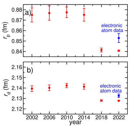
Figure 1: Comparison of the recommended value of the rms charge radii of the proton $r_{\rm p}$ and of the deuteron $r_{\rm d}$ from the 2022 and previous five CODATA adjustments (in red). Values from the 2022 adjustment are given in Table LABEL:tab:radcomp.

Table 17: Observational equations for input data on H, D, ⁴He spectroscopy of muonic-H, -D, and ⁴He Lamb shifts given in Tables 11, 12, and LABEL:tab:muhdata as functions of adjusted constants. Labels in the first column correspond to those defined in the tables with input data. Subscript $X$ is H, D, or ⁴He. Energy levels of hydrogenic atoms are discussed in Sec. III.1. Here, the symbol $\Gamma_{X}$ represents the six adjusted constants $R_{\infty},\alpha,A_{\rm r}({\rm e}),m_{\rm e}/m_{\mbox{\scriptsize{{{m}}}}},A_{\rm r}({N})$, and $r_{N}$ such that when $X={\rm H}$ the nucleus $N={\rm p}$ is the proton, when $X={\rm D}$ the nucleus $N={\rm d}$ is the deuteron, and when $X=^{4}$He the nucleus $N={\mbox{{a}}}$ is the $\alpha$ particle. The Lamb shift for muonic atoms, $\Delta{\cal E}_{\rm LS}(\mbox{{m}}X)$, is discussed in Sec. IV.

Input data	Observational equation
A1–A4, A20, A21,	$\nu_{X}({n_{1}{\ell_{1}}_{j_{1}}\!-\!n_{2}{\rm\ell_{2}}_{j_{2}}})-{\textstyle{1\over 4}}\nu_{X}({n_{3}{\ell_{3}}_{j_{3}}\!-\!n_{4}{\ell_{4}}_{j_{4}}})$	$\doteq$	$\Big{\{}E_{X}\big{(}n_{2}{\ell_{2}}_{j_{2}};\Gamma_{X}\big{)}+\delta_{X}(n_{2}{\ell_{2}}_{j_{2}})$
A24, A25			$\quad-E_{X}\big{(}n_{1}{\ell_{1}}_{j_{1}};\Gamma_{X}\big{)}-\delta_{X}(n_{1}{\ell_{1}}_{j_{1}})$
			$\quad\quad-{\textstyle{1\over 4}}\big{[}E_{X}\big{(}n_{4}{\ell_{4}}_{j_{4}};\Gamma_{X}\big{)}+\delta_{X}(n_{4}{\ell_{4}}_{j_{4}})$
			$\quad\quad\quad\quad-E_{X}\big{(}n_{3}{\ell_{3}}_{j_{3}};\Gamma_{X}\big{)}-\delta_{X}(n_{3}{\ell_{3}}_{j_{3}})\big{]}\Big{\}}/h$
A5	$\nu_{\rm D}(1{\rm S}_{1/2}\!-\!2{\rm S}_{1/2})-\nu_{\rm H}(1{\rm S}_{1/2}\!-\!2{\rm S}_{1/2})$	$\doteq$	$\Big{\{}E_{\rm D}\big{(}2{\rm S}_{1/2};\Gamma_{\rm D}\big{)}+\delta_{\rm D}(2{\rm S}_{1/2})$
			$\quad-E_{\rm D}\big{(}1{\rm S}_{1/2};\Gamma_{\rm D}\big{)}-\delta_{\rm D}(1{\rm S}_{1/2})$
			$\quad\quad-\big{[}E_{\rm H}\big{(}2{\rm S}_{1/2};\Gamma_{\rm H}\big{)}+\delta_{\rm H}(2{\rm S}_{1/2})$
			$\quad\quad\quad-E_{\rm H}\big{(}1{\rm S}_{1/2};\Gamma_{\rm H}\big{)}-\delta_{\rm H}(1{\rm S}_{1/2})\big{]}\Big{\}}/h$
A6, A7, A9–A19,	$\nu_{X}(n_{1}{\ell_{1}}_{j_{1}}\!-\!n_{2}{\ell_{2}}_{j_{2}})$	$\doteq$	$\big{[}E_{X}\big{(}n_{2}{\ell_{2}}_{j_{2}};\Gamma_{X}\big{)}+\delta_{X}(n_{2}{\ell_{2}}_{j_{2}})$
A22, A23, A26–A29			$\quad-E_{X}\big{(}n_{1}{\ell_{1}}_{j_{1}};\Gamma_{X}\big{)}-\delta_{X}(n_{1}{\ell_{1}}_{j_{1}})\big{]}/h$
A8	$\nu_{\rm H}({\rm 2S_{1/2}}\!-\!{\rm 4P,\,centroid})$	$\doteq$	$\Big{\{}\big{(}E_{\rm H}\big{(}4{\rm P}_{1/2};\Gamma_{\rm H}\big{)}+\delta_{\rm H}(4{\rm P}_{1/2})\big{)}/3$
			$\quad+2\,\big{(}E_{\rm H}\big{(}4{\rm P}_{3/2};\Gamma_{\rm H}\big{)}+\delta_{\rm H}(4{\rm P}_{3/2})\big{)}/3$
			$\quad\quad-E_{\rm H}\big{(}2{\rm S}_{1/2};\Gamma_{\rm H}\big{)}-\delta_{\rm H}(2{\rm S}_{1/2})\Big{\}}/h$
B1–B25	$\delta_{X}(n\ell_{j})$	$\doteq$	$\delta_{X}(n\ell_{j})$
C1, C3, C5	$\Delta{\cal E}_{\rm LS}(\mbox{{m}}X)$	$\doteq$	${\cal E}_{0X}+{\cal E}_{2X}\,r_{N}^{2}+\delta_{\rm th}(\mbox{{m}}X)$
C2, C4, C6	$\delta E_{\rm LS}(\mbox{{m}}X)$	$\doteq$	$\delta_{\rm th}(\mbox{{m}}X)$

V Electron magnetic-moment anomaly

The interaction of the magnetic moment of a charged lepton $\ell$ in a magnetic flux density (or magnetic field) $\bm{B}$ is described by the Hamiltonian ${\cal H}=-\bm{\mu}_{\ell}\cdot\bm{B}$, with

$$\bm{\mu}_{\ell}=g_{\ell}\,\frac{e}{2m_{\ell}}\,\bm{s},$$ (70)

where $\ell={\rm e}^{\pm}$, $\mbox{{m}}^{\pm}$, or $\mbox{{t}}^{\pm}$, $g_{\ell}$ is the $g$-factor, with the convention that it has the same sign as the charge of the particle, $e$ is the positive elementary charge, $m_{\ell}$ is the lepton mass, and $\bm{s}$ is its spin. Since the spin has projection eigenvalues of $s_{z}=\pm\hbar/2$, the magnitude of a magnetic moment is

$$\mu_{\rm\ell}=\frac{g_{\ell}}{2}\,\frac{e\hbar}{2m_{\ell}}\,.$$ (71)

The lepton magnetic-moment anomaly $a_{\ell}$ is defined by the relationship

$$|g_{\ell}| \equiv 2(1+a_{\ell})\,,$$ (72)

based on the Dirac $g$-value of $-2$ and $+2$ for the negatively and positively charged lepton $\ell$, respectively.

The Bohr magneton is defined as

$$\mu_{\rm B}=\frac{e\hbar}{2m_{\rm e}}\,,$$ (73)

and the theoretical expression for the anomaly of the electron $a_{\rm e}({\rm th})$ is

$$a_{\rm e}({\rm th})=a_{\rm e}({\rm QED})+a_{\rm e}({\rm weak})+a_{\rm e}({\rm had})\ ,$$ (74)

where terms denoted by “QED”, “weak”, and “had” account for the purely quantum electrodynamic, predominantly electroweak, and predominantly hadronic (that is, strong interaction) contributions, respectively.

The QED contribution may be written as

$$a_{\rm e}({\rm QED}) = \sum_{n=1}^{\infty}C_{\rm e}^{(2n)}\left({\alpha\over\pi}\right)^{n}\,,$$ (75)

where the index $n$ corresponds to contributions with $n$ virtual photons and

$$C_{\rm e}^{(2n)}=A^{(2n)}_{1}+A^{(2n)}_{2}(x_{{\rm e}\mbox{\scriptsize{{{m}}}}})+A^{(2n)}_{2}(x_{{\rm e}\mbox{\scriptsize{{t}}}})+\cdots$$ (76)

with mass-independent coefficients $A^{(2n)}_{1}$ and functions $A^{(2n)}_{2}(x)$ evaluated at mass ratio $x={x_{{\rm e}X}\equiv m_{\rm e}/m_{X}}\ll 1$ for lepton ${X=\mbox{{m}}}$ or t. For $n=1$, we have

$$A_{1}^{(2)} = 1/2,$$ (77)

and function ${A^{(2)}_{2}(x)=0}$, while for $n>1$ coefficients $A^{(2n)}_{1}$ include vacuum-polarization corrections with virtual electron/positron pairs. In fact,

$$A_{1}^{(4)} = -0.328\,478\,965\,579\,193\ldots\,,$$ (78)

$$A_{1}^{(6)} = 1.181\,241\,456\,587\ldots\,,$$ (79)

$$A_{1}^{(8)} = -1.912\,245\,764\ldots\,,$$ (80)

The coefficient $A^{(8)}_{1}$ has been evaluated by Laporta (2017).

Aoyama et al. (2019) have published an updated value for coefficient $A_{1}^{(10)}=6.737(159)$, reducing their uncertainty by $\approx 25$ % from that in Aoyama et al. (2018). In the same year, Volkov (2019) published an independent evaluation of the diagrams contributing to $A_{1}^{(10)}$ that have no virtual lepton loops and found $A_{1}^{(10)}[{\rm no\mathchar 45\relax lepton\mathchar 45\relax loops}]=6.793(90)$. The total coefficient $A_{1}^{(10)}=A_{1}^{(10)}[\rm no\mathchar 45\relax lepton\mathchar 45\relax loops]+A_{1}^{(10)}[\rm lepton\mathchar 45\relax loops]=5.863(90)$, where $A_{1}^{(10)}[\rm lepton\mathchar 45\relax loops]=-0.93042(361)$ from Aoyama et al. (2018) contains the contributions from diagrams that have virtual lepton loops, which have a relatively small uncertainty. All uncertainties are statistical from numerically evaluating high-dimensional integrals by Monte-Carlo methods.

The two values for $A_{1}^{(10)}$ by Volkov (2019) and Aoyama et al. (2019) are discrepant by $4.8\,\sigma$ as shown in Fig. 2, implying the need for an expansion factor for this 2022 CODATA adjustment. A least-squares fit gives normalized residuals $-2.4$ and $4.2$ for the values by Volkov (2019) and Aoyama et al. (2019), respectively, and

$$A^{(10)}_{1}\bigl{|}_{\rm CODATA\mathchar 45\relax 2022}=6.08(16)\,,$$ (81)

where we have applied an expansion factor of $2.1$ to the uncertainty used for the two input data to ensure that the values of Volkov (2019) and Aoyama et al. (2019) lie within twice their (expanded) uncertainties of the recommended value.

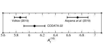
Figure 2: Coefficient $A_{1}^{(10)}$ for the electron anomaly and its uncertainty as evaluated by Aoyama et al. (2019) and Volkov (2019) as well as its value and uncertainty used in the 2022 CODATA adjustment. The values of $A_{1}^{(10)}$ used in the adjustment include an expansion factor of $2.1$ so that both values lie within two expanded standard deviations of the 2022 CODATA value.

The functions $A^{(2n)}_{2}(x)$ for $n>1$ are vacuum-polarization corrections due to heavier leptons. For $x\to 0$, we have $A^{(4)}_{2}(x)=x^{2}/45+{\cal O}(x^{4})$ and $A^{(6)}_{2}(x)=x^{2}(b_{0}+b_{1}\ln x)+{\cal O}(x^{4})$ with $b_{0}=0.593\,274\cdots$ and $b_{1}=23/135$ Laporta and Remiddi (1993); Laporta (1993). The ${\cal O}(x^{4})$ contributions are known and included in the calculations but not reproduced here. The functions $A^{(8)}_{2}(x)$ and $A^{(10)}_{2}(x)$ are also ${\cal O}(x^{2})$ for small $x$, but not reproduced here Kurz et al. (2014); Aoyama et al. (2015). Currently, terms with $n>5$ and vacuum-polarization corrections that depend on two lepton mass ratios can be neglected.

Table 18 summarizes the relevant QED coefficients and summed contributions to $C^{(2n)}_{\rm e}$ with their one-standard-deviation uncertainties where appropriate as used in the 2022 CODATA adjustment. Additional references to the original literature can be found in descriptions of previous CODATA adjustments.

Table 18: Coefficients for the QED contributions to the electron anomaly. The coefficients $A_{1}^{(2n)}$ and functions $A_{2}^{(2n)}(x)$, evaluated at mass ratios $x_{{\rm e}\mbox{\scriptsize{{{m}}}}}=m_{\rm e}/m_{\mbox{\scriptsize{{{m}}}}}$ and $x_{{\rm e}\mbox{\scriptsize{{t}}}}=m_{\rm e}/m_{\mbox{\scriptsize{{t}}}}$ for the muon and tau lepton, respectively; summed values $C^{(2n)}_{\rm e}$, based on values for lepton mass ratios from the 2022 CODATA adjustment, are listed as accurately as needed for the tests described in this article. Missing values indicate that their contributions to the electron anomaly are negligible.

$n$	$A_{1}^{(2n)}$	$A^{(2n)}_{2}(x_{{\rm e}\mbox{\scriptsize{{{m}}}}})$	$A^{(2n)}_{2}(x_{{\rm e}\mbox{\scriptsize{{t}}}})$	$C_{\rm e}^{(2n)}$
1	$1/2$	$0$	$0$	$\phantom{-}0.5$
2	$-0.328\,478\,965\,579\,193\ldots$	$\phantom{-}5.197\,386\,76(23)\times 10^{-7}$	$\phantom{-}1.837\,90(25)\times 10^{-9}$	$-0.328\,478\,444\,00$
3	$\phantom{-}1.181\,241\,456\,587\ldots$	$-7.373\,941\,70(24)\times 10^{-6}$	$-6.582\,73(79)\times 10^{-8}$	$\phantom{-}1.181\,234\,017$
4	$-1.912\,245\,764\ldots$	$\phantom{-}9.161\,970\,83(33)\times 10^{-4}$	$\phantom{-}7.428\,93(88)\times 10^{-6}$	$-1.911\,322\,138\,91(88)$
5	$\phantom{-}6.080(160)$	$-0.003\,82(39)$		$\phantom{-}6.08(16)$

The electroweak contribution is

$$a_{\rm e}({\rm weak}) = 0.030\,53(23)\times 10^{-12}$$ (82)

and is calculated as discussed in the 1998 CODATA adjustment, but with the 2022 values of the Fermi coupling constant $G_{\rm F}/(\hbar c)^{3}$ and the weak mixing angle $\theta_{\rm W}$ Workman et al. (2022).

Jegerlehner (2019) has provided updates to hadronic contributions to the electron anomaly. See also Karshenboim and Shelyuto (2021). Four such contributions have been considered. They are

$$a_{\rm e}({\rm had})= a_{\rm e}^{\rm LO,VP}({\rm had})+a_{\rm e}^{\rm NLO,VP}({\rm had})$$ (83)

$$\quad+\,a_{\rm e}^{\rm NNLO,VP}({\rm had})+a_{\rm e}^{\rm LL}({\rm had})$$

corresponding to leading-order (LO), next-to-leading-order (NLO), and next-to-next-to-leading-order (NNLO) hadronic vacuum-polarization corrections and a hadronic light-by-light (LL) scattering term, respectively. Contributions are determined from analyzing experimental cross sections for electron-positron annihilation into hadrons and tau-lepton-decay data. The values in the 2022 adjustment are

$$\begin{array}[]{r@{\ =\ }D{.}{.}{12}}a_{\rm e}^{\rm LO,VP}({\rm had})&.849(11)\times 10^{-12}\,,$\\ a_{\rm e}^{\rm NLO,VP}({\rm had})&-0.2213(12)\times 10^{-12}\,,$\\ a_{\rm e}^{\rm NNLO,VP}({\rm had})&0.028\,00(20)\times 10^{-12}\,,$\\ a_{\rm e}^{\rm LL}({\rm had})&0.0370(50)\times 10^{-12}$\end{array}$$ (84)

leading to the total hadronic contribution

$$a_{\rm e}({\rm had})=1.693(12)\times 10^{-12}\,.$$ (85)

A first-principle lattice quantum chromodynamics (QCD) evaluation of the leading-order hadronic correction $a_{\rm e}^{\rm LO,VP}({\rm had})$ to the electron anomaly was published in 2018 Borsanyi et al. (2018). The value is

$$a_{\rm e}^{\rm LO,VP}({\rm had})=1.893(26)(56)\times 10^{-12}\,,$$ (86)

where the first and second numbers in parentheses correspond to the statistical and systematic uncertainty, respectively. The systematic uncertainty is dominated by finite-volume artifacts. The combined uncertainty is six times larger than that obtained by analyzing electron-positron scattering data.

The theoretical uncertainty of the electron anomaly (apart from uncertainty in the fine-structure constant) is dominated by two contributions: the mass-independent $n=5$ QED correction and the hadronic contribution; its value is

$$u[a_{\rm e}({\rm th)}]=0.000(16)\times 10^{-12}=1.4\times 10^{-11}\,a_{\rm e}\,.$$ (87)

In 2022, Fan et al. (2023) at Northwestern University measured the electron anomaly $a_{\rm e}$ in an apparatus storing single electrons in a homogeneous magnetic field. Their value is new for our CODATA adjustments and has a 2.2 times smaller uncertainty than that reported in 2008 by a Harvard research group led by the same senior researcher, G. Gabrielse Hanneke et al. (2008). Still the theoretical uncertainty is significantly smaller than the $1.1\times 10^{-10}a_{\rm e}$ uncertainty reported by Fan et al. (2023). Following the recommendation by Fan et al. (2023), the 2022 measurement of $a_{\rm e}$ supersedes the 14-year-old datum.

The success of the 2022 measurements of $a_{\rm e}$ relied on a stable magnetic field even though their frequency ratio measurement is to a large degree independent of the actual field strength. Residual dependencies are a consequence of the fact that the anomalous and cyclotron frequencies of the electron are not measured simultaneously. Relative field drifts of $2\times 10^{-9}$/day, four times below that in Hanneke et al. (2008), allowed round-the-clock measurements and, thus, improved statistical precision. The researchers achieved this field stability by supporting a 50 mK electron trap in a mixing chamber flexibly hanging from the rest of a dilution refrigerator.

A stable magnetic field and electric fields generated by cylindrical Penning trap electrodes with appropriately chosen relative dimensions and potentials produce the trapping potential for the electron. The Penning trap is also a low-loss microwave cavity that is used to inhibit the decay rate of excited cyclotron states, here due to spontaneous emission of synchrotron radiation, by a factor of 50 to 70. Cyclotron excitations can then be detected before they decay. Nevertheless, the limits on the cavity design, leading to cavity shifts in the cyclotron frequency, and residual spontaneous emission were the two largest uncertainties in the experiment.

For the least-squares adjustment, we use the observational equations

$$a_{\rm e}({\rm exp})\doteq a_{\rm e}({\rm th})+\delta_{\rm th}({\rm e})$$ (88)

and

$$\delta_{\rm e}\doteq\delta_{\rm th}({\rm e})$$ (89)

with additive adjusted constant $\delta_{\rm th}({\rm e})$. Input data for $a_{\rm e}({\rm exp})$ is from Fan et al. (2023), while input datum $\delta_{\rm e}=0$ with $u[\delta_{\rm e}]=0.018\times 10^{-12}$ accounts for the uncertainty of the theoretical expression. The input data is entry D$1$ in Table LABEL:tab:pdata. Relevant observational equations are found in Table 31. Atom-recoil experiments, discussed in Sec. VI, form a second competitive means to determine $\alpha$.

VI Atom-recoil measurements

Atom-recoil measurements with rubidium and cesium atoms from the stimulated absorption and emission of photons are relevant for the CODATA adjustment as they determine the electron mass, the atomic mass constant, and the fine-structure constant Young et al. (1997); Peters et al. (1997); Mohr and Taylor (2000). This can be understood as follows.

First and foremost, recoil measurements determine the mass $m(X)$ of a neutral atom $X$ in kg using interferometers with atoms in superpositions of momentum states and taking advantage of the fact that photon energies can be precisely measured. Equally precise photon momenta $p$ follow from their dispersion or energy-momentum relation $E=pc$. In practice, Bloch oscillations are used to transfer a large number of photon momenta to the atoms in order to improve the sensitivity of the measurement Cladé (2015); Estey et al. (2015). Before the adoption of the revised SI on 20 May 2019, these experiments only measured the ratio $h/m(X)$, since the Planck constant $h$ was not an exactly defined constant.

Second, atom-recoil measurements are a means to determine the atomic mass constant, $m_{\rm u}=m(^{12}{\rm C})/12$, and the mass of the electron, $m_{\rm e}$, in kg. This follows, as many relative atomic masses $A_{\rm r}(X)=m(X)/m_{\rm u}$ of atoms $X$ are well known. For ⁸⁷Rb and ¹³³Cs, the relative atomic masses have a relative uncertainty smaller than $1\times 10^{-10}$ from the 2020 recommended values of the AMDC (see Table 1). The relative atomic mass of the electron can be determined even more precisely with spin-precession and cyclotron-frequency-ratio measurements on hydrogenic ${}^{12}{\rm C}^{5+}$ and ${}^{28}{\rm Si}^{13+}$ as discussed in Sec. VIII. We thus have

$$m_{\rm u}=m(X)/A_{\rm r}(X)$$ (90)

and

$$m_{\rm e}=\frac{A_{\rm r}({\rm e})}{A_{\rm r}(X)}m(X)$$ (91)

from a measurement of the mass of atom $X$.

Finally, the fine-structure constant follows from the observation that the Rydberg constant $R_{\infty}=\alpha^{2}m_{\rm e}c/2h$ has a relative standard uncertainty of $1.1\times 10^{-12}$ based on spectroscopy of atomic hydrogen discussed in Sec. III. The expression for $R_{\infty}$ can be rewritten as

$$\alpha=\sqrt{\frac{2\,hcR_{\infty}}{m(X)c^{2}}\,\frac{A_{\rm r}(X)}{A_{\rm r}(\rm e)}}$$ (92)

and a value of $\alpha$ with a competitive uncertainty can be obtained from a measurement of $m(X)$.

Two $m(X)$ or equivalently ${h/m(X)}$ measurements are input data in the current least-squares adjustment: A mass for ${\rm{}^{133}Cs}$ measured at the University of California at Berkeley, USA by Parker et al. (2018) and a mass for ${\rm{}^{87}Rb}$ measured at the Laboratoire Kastler-Brossel (LKB), France by Morel et al. (2020). The results are items D3 and D4 in Table LABEL:tab:pdata and satisfy the relevant observational equations in Table 31.

The values of ${\rm\alpha}$ inferred from the two atom-recoil measurements are shown in Fig. 3, together with those inferred from electron magnetic-moment anomaly $a_{\rm e}$ measurements. Their comparison provides a useful test of the QED-based determination of $a_{\rm e}$ and is further discussed in Sec. XV.1.

Morel et al. (2020) at LKB reduced by one order of magnitude several systematic effects identified in their 2011 measurement Bouchendira et al. (2011). Now they are able to adjust the altitude of atomic trajectories within 100 mm and suppress the effect of the Earth’s rotation. Long-term drifts in the laser beam alignment have been reduced and laser frequencies further stabilized with a Fabry–Pérot cavity and measured with a frequency comb. A lower density atomic sample was used to avoid problems with a changing refractive index and atom–atom interactions. Effects related to the Gouy phase and wave front curvature have been mitigated.

In addition, Morel et al. (2020) identified new systematic effects Bade et al. (2018); Cladé et al. (2019). The most subtle one is related to the question of how to calculate the photon momentum in a spatially distorted optical field. Moreover, in the expanding atomic cloud, a small phase shift due to the variation of the intensity perceived by the atoms is present and had to be mitigated. Finally, a correction for a frequency ramp used to compensate Doppler shifts induced by gravity had to be made. Morel et al. (2020) think that these new systematic effects could explain the $2.4\,\sigma$ discrepancy with the measurement in Bouchendira et al. (2011). Unfortunately, they could not retroactively evaluate these contributions for their 2011 measurement.

The determinations of the fine-structure constant from both the recoil measurements and the electron magnetic-moment anomaly are shown in Fig. 3. The recommended value includes an expansion factor of 2.5 on the uncertinties of both the measurement input data and the QED theory of the electron anomaly.

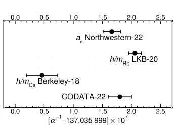
Figure 3: Determinations of the value of the fine-structure constant from atom recoil measurements and the measurement of the electron magnetic-moment anomaly. An expansion factor of 2.5 is applied to the uncertainties of these data in the adjustment, so that all values lie within two (expanded) standard deviations of the CODATA value.

VII Muon magnetic-moment anomaly

The muon magnetic-moment anomaly $a_{\mbox{\scriptsize{{{m}}}}}$ and thus the muon $g$-factor $g_{\mbox{\scriptsize{{{m}}}}}=-2(1+a_{\mbox{\scriptsize{{{m}}}}})$ were first measured in 2006, and a recent measurement was made at the Fermi National Accelerator Laboratory Abi et al. (2021). A review of the theoretical value for $a_{\mbox{\scriptsize{{{m}}}}}$ is available from the PDG Workman et al. (2022).

VII.1 Theory of the muon anomaly

The muon magnetic-moment anomaly theory is reviewed and summarized by A. Höcker (CERN) and W.J. Marciano (BNL) on p. 796 of the PDG report Workman et al. (2022). These authors conclude that there is a $4.2\,\sigma$ discrepancy between theory and experiment. Active searches for explanations for the discrepancy, which may indicate deviations from the standard model of QCD, are underway and possible such effects are discussed by Höcker and Marciano.

In view of the discrepancy and ongoing work seeking an explanation, the TGFC has decided not to include theoretical input for the recommended value of the muon magnetic-moment anomaly, so it is based on the experimental values only.

The muon magnetic-moment anomaly can be expressed as

$$a_{\mbox{\scriptsize{{{m}}}}}({\rm th})=a_{\mbox{\scriptsize{{{m}}}}}({\rm QED})+a_{\mbox{\scriptsize{{{m}}}}}({\rm weak})+a_{\mbox{\scriptsize{{{m}}}}}({\rm had})\,,$$ (93)

where terms denoted by “QED”, “weak”, and “had” account for the purely quantum electrodynamic, predominantly electroweak, and predominantly hadronic (that is, with hadrons in intermediate states) contributions, respectively.

Here, we update the QED contribution based on the CODATA 2022 recommended values of the fine-structure constant and the relevant mass ratios. It may be written as

$$a_{\mbox{\scriptsize{{{m}}}}}({\rm QED}) = \sum_{n=1}^{\infty}C_{\mbox{\scriptsize{{{m}}}}}^{(2n)}\left({\alpha\over\mbox{{p}}}\right)^{n}\,,$$ (94)

where

$$C_{\mbox{\scriptsize{{{m}}}}}^{(2n)} = A^{(2n)}_{1}+A^{(2n)}_{2}(x_{{\mbox{\scriptsize{{{m}}}}}{\rm e}})+A^{(2n)}_{2}(x_{{\mbox{\scriptsize{{{m}}}}}\mbox{\scriptsize{{t}}}})$$ (95)

$$+A^{(2n)}_{3}(x_{{\mbox{\scriptsize{{{m}}}}}\rm e},x_{{\mbox{\scriptsize{{{m}}}}}\mbox{\scriptsize{{t}}}})$$

with mass-independent coefficients $A^{(2n)}_{1}$ given by Eqs. (77)-(81) and functions $A^{(2n)}_{2}(x)$ and $A^{(2n)}_{3}(x,y)$ evaluated at mass ratios $m_{\mbox{\scriptsize{{{m}}}}}/m_{X}$ for lepton ${X=\rm e}$ or t. The expression for the QED contribution has the same functional form as that for the electron anomaly described in Sec. V, except that the mass-dependent terms $A^{(2n)}_{2}(x)$ are evaluated at different mass ratios, while contributions due to $A^{(2n)}_{3}(x,y)$ are negligibly small for the electron anomaly. Contributions from the mass-dependent terms are generally more important for the muon anomaly.

Table 19: Mass-dependent functions $A^{(2n)}_{2}(x)$, $A^{(2n)}_{3}(x,y)$, and summed $C_{\mbox{\scriptsize{{{m}}}}}^{(2n)}$ coefficients for the QED contributions to the muon anomaly based on the 2018 recommended values of lepton mass ratios. The functions are evaluated at mass ratios $x_{\mbox{\scriptsize{{{m}}}}{\rm e}}\equiv m_{\mbox{\scriptsize{{{m}}}}}/m_{\rm e}$ and/or $x_{\mbox{\scriptsize{{{m}}}}\mbox{\scriptsize{{t}}}}\equiv m_{\mbox{\scriptsize{{{m}}}}}/m_{\mbox{\scriptsize{{t}}}}$.

$n$	$A^{(2n)}_{2}(x_{\mbox{\scriptsize{{{m}}}}{\rm e}})$	$A^{(2n)}_{2}(x_{\mbox{\scriptsize{{{m}}}}\mbox{\scriptsize{{t}}}})$	$A^{(2n)}_{3}(x_{\mbox{\scriptsize{{{m}}}}{\rm e}},x_{\mbox{\scriptsize{{{m}}}}\mbox{\scriptsize{{t}}}})$	$C_{\mbox{\scriptsize{{{m}}}}}^{(2n)}$
1	$0$	$0$	$0$	$0.5$
2	$\phantom{74}1.094\,258\,3093(72)$	$\phantom{-}0.000\,078\,076(10)$	$0$	$\phantom{75}0.765\,857\,420(10)$
3	$\phantom{7}22.868\,379\,98(17)$	$\phantom{-}0.000\,360\,599(86)$	$0.000\,527\,738(71)$	$\phantom{7}24.050\,509\,77(16)$
4	$132.6852(60)$	$\phantom{-}0.042\,4928(40)$	$0.062\,72(1)$	$130.8782(60)$
5	$742.32(86)$	$-0.066(5)$	$2.011(10)$	$750.35(87)$

The mass-dependent functions $A^{(2)}_{2}(x)$, $A^{(2)}_{3}(x)$, and $A^{(4)}_{3}(x,y)$ are zero. The remaining nonzero mass-dependent coefficients computed at the relevant mass ratios are given in Table 19. Their fractional contributions to the muon anomaly are given in Table 20. Only four of the mass-dependent QED corrections contribute significantly to the theoretical value for the muon anomaly. Finally, $a_{\mbox{\scriptsize{{{m}}}}}({\rm QED})$ based on the 2022 recommended value of $\alpha$ and lepton mass ratios is

$$a_{\mbox{\scriptsize{{{m}}}}}({\rm QED})=0.001\,165\,847\,188\,14(84)\ [7.2\times 10^{-10}]\,.$$ (96)

Table 20: Fractional contribution of mass-dependent functions $A^{(2n)}_{2}(x)$ and $A^{(2n)}_{3}(x,y)$ for the QED contributions to the muon anomaly based on the 2018 recommended values for $\alpha$ and lepton mass ratios. Fractional contributions are defined as $A_{j}^{(2n)}\!\times\!(\alpha/\mbox{{p}})^{n}/a_{\mbox{\scriptsize{{{m}}}}}({\rm th})$ for $j=2$ or $3$ and the relative standard uncertainty of $a_{\mbox{\scriptsize{{{m}}}}}({\rm th})$ is $3.3\times 10^{-7}$. The functions are evaluated at mass ratios $x_{\mbox{\scriptsize{{{m}}}}{\rm e}}\equiv m_{\mbox{\scriptsize{{{m}}}}}/m_{\rm e}$ and/or $x_{\mbox{\scriptsize{{{m}}}}\mbox{\scriptsize{{t}}}}\equiv m_{\mbox{\scriptsize{{{m}}}}}/m_{\mbox{\scriptsize{{t}}}}$.

$n$	$A^{(2n)}_{2}(x_{\mbox{\scriptsize{{{m}}}}{\rm e}})$	$A^{(2n)}_{2}(x_{\mbox{\scriptsize{{{m}}}}\mbox{\scriptsize{{t}}}})$	$A^{(2n)}_{3}(x_{\mbox{\scriptsize{{{m}}}}{\rm e}},x_{\mbox{\scriptsize{{{m}}}}\mbox{\scriptsize{{t}}}})$
2	$5.06\times 10^{-3}$	$\ 3.61\times 10^{-7}$
3	$2.46\times 10^{-4}$	$\ 3.88\times 10^{-9}$	$5.67\times 10^{-9}$
4	$3.31\times 10^{-6}$	$\ 1.06\times 10^{-9}$	$1.57\times 10^{-9}$
5	$4.31\times 10^{-8}$	$-3.80\times 10^{-12}$	$1.17\times 10^{-10}$

For the electroweak and hadronic corrections to the muon anomaly, we follow the recommendations of the PDG PDG Workman et al. (2022). The primarily electroweak contribution is

$$a_{\mbox{\scriptsize{{{m}}}}}{({\rm weak})} = 153.6(1.0)\times 10^{-11}$$ (97)

and contains both the leading term and also some higher-order corrections. The PDG value of the hadronic corrections is

$$a_{\mbox{\scriptsize{{{m}}}}}({\rm had}) = 6937(44)\,,$$ (98)

which yields a total theoretical value of

$$a_{\mbox{\scriptsize{{{m}}}}}({\rm th}) = 1.165\,918\,09(44)\times 10^{-3}\,.$$ (99)

VII.2 2006 Measurement of the muon anomaly at Brookhaven National Laboratory

The 2006 determination of the muon anomaly Bennett et al. (2006) at Brookhaven National Laboratory (BNL), USA in a 1.45 T superconducting storage ring magnet with an approximate diameter of 7 m has been discussed in past CODATA adjustment reports. The relativistic velocity of the muons in the ring is chosen such that the dependence on the static electric field used for transverse confinement is tuned out. The spread in their velocities leads to a negligible contribution to the uncertainty budget. The quantity measured is the anomaly difference frequency $\omega_{\rm a}=\omega_{\rm s}-\omega_{\rm c}$, where $\omega_{\rm s}=|g_{\mbox{\scriptsize{{{m}}}}}|(e/2m_{\mbox{\scriptsize{{{m}}}}})B$ is the muon spin-flip (or precession) frequency in applied magnetic flux density $B$ and $\omega_{\rm c}=(e/m_{\mbox{\scriptsize{{{m}}}}})B$ is the muon cyclotron frequency.

The magnetic flux density was eliminated from these expressions by determining its value from a measurement of the precession frequency of the shielded proton in a spherical sample of pure H₂O in the same apparatus, which depends on the temperature of the H₂O.

Bennett et al. (2006) in Table XV give as the result of their experiment $R_{\mbox{\scriptsize{{{m}}}}}=\omega_{a}/\omega_{\rm p}=0.003\,707\,2063(20)~{}[5.4\times 10^{-7}]$, where $\omega_{\rm p}$ is the precession frequency of the free proton. This value, to which consistent measurements on both positively and negatively charged muons contributed, was used as the input datum for the BNL experiment in the 2006, 2010, 2014, and 2018 CODATA adjustments. Nevertheless, it was decided for the 2022 adjustment to treat the BNL result in the same way other data involving the shielded proton are treated, including the result reported in 2021 from the similar experiment carried out at the Fermi National Accelerator Laboratory (FNAL) in Batavia, Illinois, USA. It is discussed in the next section.

Bennett et al. (2006) (see section IV.A.1 of their paper) obtained the above free proton value by converting their (unreported) result to the free proton value based on the measurements of the shielding by Phillips et al. (1977) and the temperature dependence measured by Petley and Donaldson (1984).

In previous CODATA adjustments, except for the value of $R_{\mbox{\scriptsize{{{m}}}}}$, all input data involving the precession frequency of protons in a spherical pure H₂O sample obtained at a temperature other than $25\,^{\circ}$C are converted to the reference temperature $25\,^{\circ}$C using the expression obtained experimentally by Petley and Donaldson given in Eq. (104) in the next section. Further, the adjusted constants that depend on the shielded proton are taken to be for protons in a spherical sample of pure H₂O at $25\,^{\circ}$C. For such converted input data and adjusted constants, no temperature is specified but a prime alone is used. For example, $\omega_{\rm p}^{\prime}$ and $\mu_{\rm p}^{\prime}$ are the shielded proton precession frequency and the shielded proton magnetic moment for protons in a spherical sample of pure H₂O at $25\,^{\circ}$C, respectively.

Converting the Bennett et al. (2006) reported value to $25\,^{\circ}$C yields

$$R_{\mbox{\scriptsize{{{m}}}}}^{\prime}({\rm BNL})=\omega_{a}/\omega^{\prime}_{\rm p}$$

$$\qquad\qquad=0.003\,707\,3015(20)~{}[5.4\times 10^{-7}]\,.$$ (100)

The relevant observational equation is

$$R^{\prime}_{\mbox{\scriptsize{{{m}}}}}=\frac{e\hbar/(2m_{\mbox{\scriptsize{{{m}}}}})}{\mu^{\prime}_{\rm p}}a_{\mbox{\scriptsize{{{m}}}}} \doteq -\frac{a_{\mbox{\scriptsize{{{m}}}}}}{1+a_{\rm e}({\rm th})+\delta_{\rm th}({\rm e})}\frac{m_{\rm e}}{m_{\mbox{\scriptsize{{{m}}}}}}\frac{\mu_{\rm e}}{\mu^{\prime}_{\rm p}}\,,\qquad$$ (101)

where the adjusted constants are $a_{\mbox{\scriptsize{{{m}}}}}$, $m_{\rm e}/m_{\mbox{\scriptsize{{{m}}}}}$, and $\mu_{\rm e}/\mu^{\prime}_{\rm p}$, as well as the additive correction $\delta_{\rm th}({\rm e})$ for the theoretical anomaly of the electron.

VII.3 2021 Measurement of the muon anomaly at the Fermi National Accelerator Laboratory (FNAL)

New for the 2022 CODATA adjustment is a measurement of the anomaly of the positively charged muon $a_{\mbox{\scriptsize{{{m}}}}}$ from FNAL Abi et al. (2021). It uses the same 1.45 T superconducting storage ring magnet but has a 2.5 times improved uniformity of the magnetic flux density. Moreover, metrology for beam properties and the characterization of positrons, a decay product of the muon, have been improved. The apparatus operates in a pulsed mode, where every 1.4 s a compact bunch of about 5000 muons are prepared and stored in the ring. The velocity of the muons is again tuned such that the dependence on electric fields, used for transverse confinement, cancels in the expression for the spin precession frequency. The result of the FNAL experiment run 1 as reported by Abi et al. (2021) is

$$R_{\mbox{\scriptsize{{{m}}}}}^{\prime}(34.7\,^{\circ}{\rm C})_{\rm FNAL}=\omega_{a}/\omega^{\prime}_{\rm p}(34.7\,^{\circ}{\rm C})$$

$$\qquad\qquad=0.003\,707\,3003(17)~{}[4.6\times 10^{-7}]\,,$$ (102)

where the reference temperature of $34.7\,^{\circ}{\rm C}$ reported for the magnetic field calibration is the same as that used by Phillips et al. (1977). Conversion of this value to the reference value of $25\,^{\circ}{\rm C}$ yields

$$R^{\prime}_{\mbox{\scriptsize{{{m}}}}}({\rm FNAL})=\omega_{a}/\omega^{\prime}_{\rm p}$$

$$\qquad\qquad=0.003\,707\,2999(17)\quad[4.6\times 10^{-7}]\,.$$ (103)

Its observational equation is Eq. (101), the same as for $R^{\prime}_{\mbox{\scriptsize{{{m}}}}}({\rm BNL})$.

The input data and observational equation for both muon-anomaly experiments can also be found in Table LABEL:tab:pdata and Table 31, respectively.

The quantity $R_{\mbox{\scriptsize{{{m}}}}}^{\prime}({\rm FNAL})$, which is input datum D34 in Table LABEL:tab:pdata, is one of five input data whose determination involved measuring the precession frequency of shielded protons in a sample of pure H₂O. The other four are D33, $R_{\mbox{\scriptsize{{{m}}}}}^{\prime}({\rm BNL})$; D43, $\mu_{\rm e}(\mbox{H})/\mu_{\rm p}^{\prime}$; D44, $\mu_{\rm h}(^{3}\mbox{He})/\mu_{\rm p}^{\prime}$ (former symbol $\mu_{\rm h}^{\prime}/\mu_{\rm p}^{\prime}$); and D46, $\mu_{\rm n}/\mu_{\rm p}^{\prime}$. For D33, D34, and D43 the temperature reported for the sample was $34.7\,^{\circ}{\rm C}$, for D44 it was $25\,^{\circ}$C and hence no conversion is necessary, and for D46 the temperature was $22\,^{\circ}$C. The conversion factor is obtained from the experimentally derived expression of Petley and Donaldson (1984) valid over the temperature range $5\,^{\circ}{\rm C}$ to $45\,^{\circ}{\rm C}$:

$$\frac{\mu_{\rm p}^{\prime}(t)}{\mu_{\rm p}^{\prime}} = 1-10.36(30)\times 10^{-9}\,\frac{(t-25\,^{\circ}\mbox{C})}{{}^{\circ}\mbox{C}}\,,$$ (104)

with $t=34.7\,^{\circ}{\rm C}$ or $t=22\,^{\circ}{\rm C}$. Thus

$$\frac{\mu_{\rm p}^{\prime}(34.7\,^{\circ}{\rm C})}{\mu_{\rm p}^{\prime}} = 0.999\,999\,8995(29)\,[2.9\times 10^{-9}]\,,$$

$$\frac{\mu_{\rm p}^{\prime}(22\,^{\circ}{\rm C})}{\mu_{\rm p}^{\prime}} = 1.000\,000\,031\,08(90)\,[9.0\times 10^{-10}]\,.\qquad$$ (105)

The relative uncertainties of D33, D34, D43, and D46 before conversion are $5.4\times 10^{-7}$, $4.6\times 10^{-7}$, $1.0\times 10^{-8}$, and $2.4\times 10^{-7}$, respectively. For D33 and D34, the $2.9\times 10^{-9}$ uncertainty of its conversion factor is more than two orders of magnitude smaller than their relative uncertainties and is entirely negligible. This is also the case for the uncertainty of D46 and the $9.0\times 10^{-10}$ uncertainty of its conversion factor. However, the $2.9\times 10^{-9}$ uncertainty of the conversion factor for D43 is not negligible compared to its $1.0\times 10^{-8}$ uncertainty and increases its relative uncertainty from $1.0\times 10^{-8}$ to $1.1\times 10^{-8}$.

We conclude this section by noting that on 11 August 2023, some seven months after the 31 December 2022 closing date for new data for the 2022 adjustment, the FNAL Muon $g-2$ Collaboration posted the preprint arXiv:2308.06230v1 on the archive server at https://arxiv.org. It not only reports new values of $R_{\mbox{\scriptsize{{{m}}}}}^{\prime}(34.7\,^{\circ}$C) obtained from runs 2 and 3, but in reference 23 updates the run-1 value in Eq. (102) by the fractional amount $+0.28\times 10^{-7}$. However, this correction is small compared with the $4.6\times 10^{-7}$ relative uncertainty of the run-1 value and only increases the last digit of that value from 3 to 4. The preprint, subsequently published Aguillard et al. (2023), also gives as the combined result from all three runs as $0.003\,707\,300\,82(75)\ [2.0\times 10^{-7}]$. The value in Eq. (102), which is the basis of the input datum in Eq. (103), is in excellent agreement with this result but its uncertainty is 2.3 times larger. Nevertheless, it means that the numerical value of the 2022 recommended experimental value of $a_{\mbox{\scriptsize{{{m}}}}}$ should not be significantly different from that which would result if the new three-run result had been available by the closing date.

VII.4 Comparison of experiment and theory

The combined experimental value for $a_{\mbox{\scriptsize{{{m}}}}}$(exp) is

$$a_{\mbox{\scriptsize{{{m}}}}}{\rm(exp)} = 0.001\,165\,920\,62(41)\times 10^{-3}\,,$$ (106)

which is the recommended value. Comparison to Eq. (99) yields

$$a_{\mbox{\scriptsize{{{m}}}}}{\rm(exp)}-a_{\mbox{\scriptsize{{{m}}}}}{\rm(th)}=253(60)\times 10^{-11}\,,$$ (107)

corresponding to the $4.2\,\sigma$ disagreement mentioned at the beginning of Sec. VII.1 above.

VIII Atomic $g$-factors in hydrogenic ¹²C and ²⁸Si ions

The most accurate value for the relative atomic mass of the electron is obtained from measurements of the ratio of spin-precession and cyclotron frequencies in hydrogenic carbon and silicon and theoretical expressions for the $g$-factors of their bound electron. See, for example, the recent analysis by Zatorski et al. (2017). These measurements also play an important role in determining the fine-structure constant using atom-recoil experiments discussed in Sec. VI.

For a hydrogenic ion $X$ in its electronic ground state 1S_1/2 and with a spinless nucleus, the Hamiltonian in an applied magnetic flux density $\bm{B}$ is

$${\cal H} = -g_{\rm e}(X)\,\frac{e}{2m_{\rm e}}\,{\bm{J}}\cdot{\bm{B}}\,,$$ (108)

where ${\bm{J}}$ is the electron angular momentum and $g_{\rm e}(X)$ is the bound-state $g$-factor for the electron. The electron angular momentum projection is $J_{z}=\pm\hbar/2$ along the direction of $\bm{B}$, so the energy splitting between the two levels is

$$\Delta E=|g_{\rm e}(X)|\,\frac{e\hbar}{2m_{\rm e}}\,B,$$ (109)

and the spin-flip precession frequency is

$$\omega_{\rm s}=\frac{\Delta E}{\hbar}=|g(X)|\,\frac{eB}{2m_{\rm e}}.$$ (110)

The ion’s cyclotron frequency is

$$\omega_{\rm c} = \frac{q_{X}B}{m_{X}}\,,$$ (111)

where $q_{X}=(Z-1)e$, $Z$, and $m_{X}$ are its net charge, atomic number, and mass, respectively. The frequency ratio $\omega_{\rm s}/\omega_{\rm c}$ is then independent of $\bm{B}$ and satisfies

$$\frac{\omega_{\rm s}}{\omega_{\rm c}}=\frac{|g_{\rm e}(X)|}{2(Z-1)}\,\frac{m_{X}}{m_{\rm e}}=\frac{|g_{\rm e}(X)|}{2(Z-1)}\,\frac{A_{\rm r}(X)}{A_{\rm r}({\rm e})}\,,$$ (112)

where $A_{\rm r}(X)$ is the relative atomic mass of the ion.

We summarize the theoretical computations of the $g$-factor in Sec. VIII.1 and describe the experimental input data and observational equations in Secs. VIII.2 and VIII.3.

VIII.1 Theory of the bound-electron $g$-factor

The bound-electron $g$-factor is given by

$$g_{\rm e}(X)=g_{\rm D}+\Delta g_{\rm rad}+\Delta g_{\rm rec}+\Delta g_{\rm ns}+\cdots\ ,$$ (113)

where the individual terms on the right-hand side are the Dirac value, radiative corrections, recoil corrections, and nuclear-size corrections, and the dots represent possible additional corrections not already included.

The Dirac value is Breit (1928)

$$g_{\rm D} = -\frac{2}{3}\left[1+2\sqrt{1-(Z\alpha)^{2}}\right]$$

$$= -2\left[1-\frac{1}{3}(Z\alpha)^{2}-\frac{1}{12}(Z\alpha)^{4}-\frac{1}{24}(Z\alpha)^{6}+\cdots\right]\,,$$

where the only uncertainty is due to that in $\alpha$.

The radiative correction is given by the series

$$\Delta g_{\rm rad}=\sum_{n=1}^{\infty}\Delta g^{(2n)}\,,$$ (115)

where

$$\Delta g^{(2n)} = -2\,C_{\rm e}^{(2n)}(Z\alpha)\left({\alpha\over\mbox{{p}}}\right)^{n}\,.$$ (116)

The first or one-photon coefficient in the series has self-energy (SE) and vacuum-polarization (VP) contributions, i.e., $C_{\rm e}^{(2)}(Z\alpha)=C_{\rm e,SE}^{(2)}(Z\alpha)+C_{\rm e,VP}^{(2)}(Z\alpha)$. The self-energy coefficient is Grotch (1970); Faustov (1970); Close and Osborn (1971); Pachucki et al. (2004, 2005)

$$C_{\rm e,SE}^{(2)}(Z\alpha) = \frac{1}{2}\,\bigg{\{}1+\frac{(Z\alpha)^{2}}{6}+(Z\alpha)^{4}\left[\frac{32}{9}\,\ln(Z\alpha)^{-2}\right.$$ (117)

$$\left.+\frac{247}{216}-\frac{8}{9}\,\ln{k_{0}}-\frac{8}{3}\,\ln{k_{3}}\right]$$

$$+(Z\alpha)^{5}\,R_{\rm SE}(Z\alpha)\bigg{\}}\ ,$$

where

$$\ln{k_{0}} = 2.984\,128\,556\,,$$ (118)

$$\ln{k_{3}} = 3.272\,806\,545\,,$$ (119)

$$R_{\rm SE}(6\alpha) = 22.1660(10)\,,$$ (120)

$$R_{\rm SE}(14\alpha) = 21.000\,5(1)\,.$$ (121)

Values for the remainder function $R_{\rm SE}(Z\alpha)$ for carbon and silicon have been taken from Yerokhin and Harman (2017). Pachucki and Puchalski (2017) have shown that

$$R_{\rm SE}(0)=\pi\left\{\frac{89}{16}+\frac{8}{3}\ln 2\right\}\,.$$ (122)

Finally, we have

$$\begin{array}[]{rcl}C_{\rm e,SE}^{(2)}(6\alpha)&=&0.500\,183\,607\,131(80)\,,\\ C_{\rm e,SE}^{(2)}(14\alpha)&=&0.501\,312\,638\,14(56)\,.\end{array}$$ (123)

The lowest-order vacuum-polarization coefficient $C_{\rm e,VP}^{(2)}(Z\alpha)$ has a wave-function and a potential contribution, each of which can be separated into a lowest-order Uehling-potential contribution and a higher-order Wichmann-Kroll contribution. The wave-function correction is Beier (2000); Beier et al. (2000); Karshenboim (2000); Karshenboim et al. (2001a, b)

$$\begin{array}[]{rcl}C_{\rm e,VPwf}^{(2)}(6\alpha)&=&-0.000\,001\,840\,3431(43)\,,\\ C_{\rm e,VPwf}^{(2)}(14\alpha)&=&-0.000\,051\,091\,98(22)\,.\end{array}$$ (124)

For the potential correction, the Uehling contribution vanishes Beier et al. (2000), and for the Wichmann-Kroll part we take the value of Lee et al. (2005), which has a negligible uncertainty from omitted binding corrections for the present level of uncertainty. This leads to

$$\begin{array}[]{rcl}C_{\rm e,VPp}^{(2)}(6\alpha)&=&0.000\,000\,008\,201(11)\,,\\ C_{\rm e,VPp}^{(2)}(14\alpha)&=&0.000\,000\,5467(11)\,,\end{array}$$ (125)

and for the total lowest-order vacuum-polarization coefficient

$$\begin{array}[]{rcl}C_{\rm e,VP}^{(2)}(6\alpha)&=&-0.000\,001\,832\,142(12)\,,\\ C_{\rm e,VP}^{(2)}(14\alpha)&=&-0.000\,050\,5452(11)\,.\end{array}$$ (126)

Moreover, we have

$$C_{\rm e}^{(2)}(6\alpha) = C_{\rm e,SE}^{(2)}(6\alpha)+C_{\rm e,VP}^{(2)}(6\alpha)$$

$$= 0.500\,181\,774\,989(81)\,,$$

$$C_{\rm e}^{(2)}(14\alpha) = C_{\rm e,SE}^{(2)}(14\alpha)+C_{\rm e,VP}^{(2)}(14\alpha)$$ (127)

$$= 0.501\,262\,0929(12)\,.$$

The two-photon $n=2$ correction factor for the ground S state is Pachucki et al. (2005); Jentschura et al. (2006)

$$C_{\rm e}^{(4)}(Z\alpha) = \left(1+{(Z\alpha)^{2}\over 6}\right)C_{\rm e}^{(4)}+(Z\alpha)^{4}$$ (128)

$$\times\bigg{[}\frac{14}{9}\,\ln(Z\alpha)^{-2}+\frac{991\,343}{155\,520}-\frac{2}{9}\,\ln{k_{0}}$$

$$-\frac{4}{3}\,\ln{k_{3}}+\frac{679\,\mbox{{p}}^{2}}{12\,960}-\frac{1441\,\mbox{{p}}^{2}}{720}\,\ln{2}$$

$$+\frac{1441}{480}\,\zeta({3})+\frac{16-19\mbox{{p}}^{2}}{216}\bigg{]}+(Z\alpha)^{5}$$

$$\times\bigg{[}{\frac{14\mbox{{p}}}{135}\,\ln(Z\alpha)^{-2}}+\frac{1}{2}\,R^{(4)}(Z\alpha)\bigg{]}\,,$$

where $C_{\rm e}^{(4)}=-0.328\,478\,444\,00\ldots$. The last term in square brackets for the contribution of order $(Z\alpha)^{4}$ is a light-by-light scattering contribution Czarnecki and Szafron (2016). The first term in square brackets for the contribution of order $(Z\alpha)^{5}$, absent in the previous adjustment, is also a light-by-light scattering contribution Czarnecki et al. (2020).

The term $(Z\alpha)^{5}R^{(4)}(Z\alpha)$ in Eq. (128) is the contribution of order $(Z\alpha)^{5}$ and higher from diagrams with zero, one, or two vacuum-polarization loops. Yerokhin and Harman (2013) have performed nonperturbative calculations for many of the vacuum-polarization contributions to this function, denoted here by $R^{(4)}_{\rm VP}(Z\alpha)$, with the results

$$R^{(4)}_{\rm VP}(6\alpha)=14.28(39)\,,\quad R^{(4)}_{\rm VP}(14\alpha)=12.72(4)$$ (129)

for the two ions. These vacuum-polarization values are the sum of three contributions. The first, denoted with subscript SVPE, is from self-energy vertex diagrams with a free-electron vacuum-polarization loop included in the photon line and magnetic interactions on the bound-electron line. This calculation involves severe numerical cancellations when lower-order terms are subtracted for small $Z$. The results

$$R^{(4)}_{\rm SVPE}(6\alpha)=0.00(15)\,,\quad R^{(4)}_{\rm SVPE}(14\alpha)=-0.152(43)$$ (130)

were extrapolated from results for $Z\geq 20$. The second contribution, denoted with subscript SEVP, is from screening-like diagrams with separate self-energy and vacuum-polarization loops. The vacuum-polarization loop includes the higher-order Wichmann-Kroll terms and magnetic interactions are only included in the bound-electron line. This set gives

$$R^{(4)}_{\rm SEVP}(6\alpha)=7.97(36)\,,\quad R^{(4)}_{\rm SEVP}(14\alpha)=7.62(1)\,.$$ (131)

The third contribution, denoted with subscript VPVP, comes from twice-iterated vacuum-polarization diagrams and from the Källén-Sabry corrections with free-electron vacuum-polarization loops, all with magnetic interactions on the bound-electron line. This set gives

$$R^{(4)}_{\rm VPVP}(6\alpha)=6.31\,,\quad R^{(4)}_{\rm VPVP}(14\alpha)=5.25\,.$$ (132)

The results for this latter contribution are consistent with a perturbative result at $Z\alpha=0$ given by Jentschura (2009)

$$R^{(4)}_{\rm VPVP}(0) = \left(\frac{1\,420\,807}{238\,140}+\frac{832}{189}\,\ln{2}-\frac{400}{189}\,\mbox{{p}}\right)\mbox{{p}}$$ (133)

$$= 7.4415\dots\,.$$

Czarnecki et al. (2018) performed perturbative calculations at $Z\alpha=0$ for a complementary set of diagrams contributing to $R^{(4)}(Z\alpha)$. These calculations include self-energy diagrams without vacuum-polarization loops, with the combined result

$$\Delta R^{(4)}(0)=4.7304(9)\,.$$ (134)

This value has three contributions. One is from self-energy diagrams without vacuum-polarization loops given by

$$R^{(4)}_{\rm SE}(0)=0.587\,35(9)\,\mbox{{p}}^{2}\,.$$ (135)

The second set has light-by-light diagrams with nuclear interactions in a vacuum-polarization loop inserted into the photon line in a self-energy diagram, which gives

$$R^{(4)}_{\rm LBL}(0)=-0.172\,452\,6(1)\,\mbox{{p}}^{2}\,.$$ (136)

The remaining contribution with external magnetic-field coupling to a virtual-electron loop is given by

$$R^{(4)}_{\rm ML}(0) = \left(-\frac{101\,698\,907}{3\,402\,000}+\frac{92\,368}{2\,025}\,\ln{2}-\frac{7\,843}{16\,200}\,\mbox{{p}}\right)\mbox{{p}}$$ (137)

$$= 0.064\,387\dots\mbox{{p}}^{2}\,.$$

The results by Yerokhin and Harman (2013) and Czarnecki et al. (2018) can be combined to give

$$R^{(4)}(Z\alpha) = R^{(4)}_{\rm VP}(Z\alpha)+\Delta R^{(4)}(0)\,,$$ (138)

which has uncertainty computed in quadrature from that of $R^{(4)}_{\rm VP}(Z\alpha)$ and, following Czarnecki et al. (2018),

$$u\left[\Delta R^{(4)}(0)\right]=\left|Z\alpha\,\ln^{3}{(Z\alpha)^{2}}\right|$$ (139)

taken to be on the order of the contribution of the next-order term. For $Z=6$ and $14$, this uncertainty is approximately twice $\Delta R^{(4)}(0)$. Finally, we have for the two-photon coefficients

$$\begin{array}[]{rcl}C_{\rm e}^{(4)}(6\alpha)&=&-0.328\,579\,27(86)\\ C_{\rm e}^{(4)}(14\alpha)&=&-0.329\,171(54).\end{array}$$ (140)

For $n>2$ contributions $\Delta g^{(2n)}$ to the radiative correction, it is sufficient to use the observations of Eides and Grotch (1997) and Czarnecki et al. (2000), who showed that

$$C_{\rm e}^{(2n)}(Z\alpha)=\left(1+{(Z\alpha)^{2}\over 6}+\cdots\right)C_{\rm e}^{(2n)}$$ (141)

for all $n$. The values for constants $C_{\rm e}^{(2n)}$ for $n=1$ through 5 are given in Table 18. This dependence for $n=1$ and 2 can be recognized in Eqs. (117) and (140), respectively. For $n=3$ we use

$$\begin{array}[]{rcl}C_{\rm e}^{(6)}(Z\alpha)&=&1.181\,611\ldots\quad{\rm for}~{}Z=6,\\ &=&1.183\,289\ldots\quad{\rm for}~{}Z=14\,,\end{array}$$ (142)

while for $n=4$ we have

$$\begin{array}[]{rcl}C_{\rm e}^{(8)}(Z\alpha)&=&-1.911\,933\dots\ {\rm for}~{}Z=6,\\ &=&-1.914\,647\dots\ {\rm for}~{}Z=14\,,\end{array}$$ (143)

and, finally, for $n=5$

$$\begin{array}[]{rcl}C_{\rm e}^{(10)}(Z\alpha)&=&6.08(16)\quad{\rm for}~{}Z=6\\ &=&6.09(16)\quad{\rm for}~{}Z=14\,.\end{array}$$ (144)

Recoil of the nucleus gives a correction $\Delta g_{\rm rec}$ proportional to the electron-nucleus mass ratio and can be written as $\Delta g_{\rm rec}=\Delta g_{\rm rec}^{(0)}+\Delta g_{\rm rec}^{(2)}+\dots$ , where the two terms are zero and first order in $\alpha/\mbox{{p}}$, respectively. The first term is Shabaev and Yerokhin (2002); Eides and Grotch (1997)

$$\Delta g_{\rm rec}^{(0)} = \bigg{\{}-(Z\alpha)^{2}+{(Z\alpha)^{4}\over 3[1+\sqrt{1-(Z\alpha)^{2}}]^{2}}$$

$$-(Z\alpha)^{5}\,P(Z\alpha)\bigg{\}}{m_{\rm e}\over m_{N}}+(1+Z)(Z\alpha)^{2}\left({m_{\rm e}\over m_{N}}\right)^{\!2}\,,$$

where $m_{N}$ is the mass of the nucleus. Mass ratios, based on the current adjustment values of the constants, are ${m_{\rm e}/m(^{12}{\rm C}^{6+})}=0.000\,045\,727\,5\ldots$ and ${m_{\rm e}/m(^{28}{\rm Si}^{14+})}=0.000\,019\,613\,6\ldots$. For carbon $P(6\alpha)=10.493\,96(1)$, and for silicon $P(14\alpha)=7.162\,26(1)$ Malyshev et al. (2020).

For $\Delta g_{\rm rec}^{(2)}$ we have

$$\Delta g_{\rm rec}^{(2)} = {\alpha\over\mbox{{p}}}{(Z\alpha)^{2}\over 3}{m_{\rm e}\over m_{N}}+\cdots\,.$$ (146)

The uncertainty in $\Delta g_{\rm rec}^{(2)}$ is negligible compared to that of $\Delta g_{\rm rad}^{(2)}$.

Glazov and Shabaev (2002) have calculated the nuclear-size correction $\Delta g_{\rm ns,LO}$ within lowest-order perturbation theory based on a homogeneous-sphere nuclear-charge distribution and Dirac wave functions for the electron bound to a point charge. To good approximation, the correction is Karshenboim (2000)

$$-{8\over 3}(Z\alpha)^{4}\left({R_{N}\over\lambda\hskip-4.5pt\vrule height=4.6pt,depth=-4.3pt,width=4.0pt_{\rm C}}\right)^{2},$$ (147)

where $R_{N}$ is the rms nuclear charge radius and $\lambda\hskip-4.5pt\vrule height=4.6pt,depth=-4.3pt,width=4.0pt_{\rm C}$ is the reduced Compton wavelength of the electron. In the CODATA adjustment, we scale the values of Glazov and Shabaev (2002) with the squares of updated values for the nuclear radii $R_{N}=2.4702(22)$ fm and $R_{N}=3.1224(24)$ fm from the compilation of Angeli and Marinova (2013) for ¹²C and ²⁸Si, respectively.

Recently, higher-order contributions of the nuclear-size correction have been computed by Karshenboim and Ivanov (2018a). They are

$$\Delta g_{\rm ns,NLO}=-\left(\frac{2}{3}Z\alpha{R_{N}\over\lambda\hskip-4.5pt\vrule height=4.6pt,depth=-4.3pt,width=4.0pt_{\rm C}}C_{\rm ZF}+\frac{\alpha}{4\mbox{{p}}}\right)\Delta g_{\rm ns,LO}\,,$$ (148)

where $C_{\rm ZF}=3.3$ is the ratio of the Zemach or Friar moment Friar and Payne (1997) to $R_{N}^{3}$ for a homogeneous-sphere nuclear-charge distribution. We assume that $\Delta g_{\rm ns,NLO}$ has a 10 % uncertainty.

The sum of the scaled nuclear-size correction of Glazov and Shabaev (2002) and Eq. (148) yields

$$\begin{array}[]{rcl}\Delta g_{\rm ns}&=&-0.000\,000\,000\,407(1)\quad{\rm for}~{}^{12}{\rm C}^{5+}\,,\\ \Delta g_{\rm ns}&=&-0.000\,000\,020\,48(3)\quad\,\ {\rm for}~{}^{28}{\rm Si}^{13+}\end{array}$$ (149)

for the total nuclear-size correction.

Table 21: Theoretical contributions and total value for the $g$-factor of hydrogenic ¹²C⁵⁺ based on the 2022 recommended values of the constants.

Contribution	Value	Source
Dirac $g_{\rm D}$	$-1.998\,721\,354\,392\,8(4)$	Eq. (VIII.1)
$\Delta g^{(2)}_{\rm SE}$	$-0.002\,323\,672\,436\,6(5)$	Eq. (123)
$\Delta g^{(2)}_{\rm VP}$	$\phantom{-}0.000\,000\,008\,511$	Eq. (126)
$\Delta g^{(4)}$	$\phantom{-}0.000\,003\,545\,6925(93)$	Eq. (140)
$\Delta g^{(6)}$	$-0.000\,000\,029\,618$	Eq. (142)
$\Delta g^{(8)}$	$\phantom{-}0.000\,000\,000\,111$	Eq. (143)
$\Delta g^{(10)}$	$-0.000\,000\,000\,001$	Eq. (144)
$\Delta g_{\rm rec}$	$-0.000\,000\,087\,629$	Eqs. (VIII.1) and (146)
$\Delta g_{\rm ns}$	$-0.000\,000\,000\,407(1)$	Eq. (149)
$g(^{12}{\rm C}^{5+})$	$-2.001\,041\,590\,1691(94)\vbox to12.0pt{}$	Eq. (150)

Table 22: Theoretical contributions and total value for the $g$-factor of hydrogenic ²⁸Si¹³⁺ based on the 2022 recommended values of the constants.

Contribution	Value	Source
Dirac $g_{\rm D}$	$-1.993\,023\,571\,561(2)$	Eq. (VIII.1)
$\Delta g^{(2)}_{\rm SE}$	$-0.002\,328\,917\,507(3)$	Eq. (123)
$\Delta g^{(2)}_{\rm VP}$	$\phantom{-}0.000\,000\,234\,81(1)$	Eq. (126)
$\Delta g^{(4)}$	$\phantom{-}0.000\,003\,552\,08(58)$	Eq. (140)
$\Delta g^{(6)}$	$-0.000\,000\,029\,66$	Eq. (142)
$\Delta g^{(8)}$	$\phantom{-}0.000\,000\,000\,11$	Eq. (143)
$\Delta g^{(10)}$	$-0.000\,000\,000\,00$	Eq. (144)
$\Delta g_{\rm rec}$	$-0.000\,000\,205\,88$	Eqs. (VIII.1)-(146)
$\Delta g_{\rm ns}$	$-0.000\,000\,020\,48(3)$	Eq. (149)
$g(^{28}{\rm Si}^{13+})$	$-1.995\,348\,958\,08(58)\vbox to12.0pt{}$	Eq. (150)

Tables 21 and 22 list the contributions discussed above to $g_{\rm e}(X)$ for $X=^{12}$C⁵⁺ and ²⁸Si¹³⁺, respectively. The final values are

$$\begin{array}[]{rcl}g_{\rm e}(^{12}{\rm C}^{5+})&=&-2.001\,041\,590\,1691(94)\,,\\ g_{\rm e}(^{28}{\rm Si}^{13+})&=&-1.995\,348\,958\,08(58)\end{array}$$ (150)

with uncertainties that are dominated by that of the two-photon radiative correction $\Delta g^{(4)}$. This uncertainty is dominated by terms proportional to $(Z\alpha)^{6}$ multiplying various powers of $\ln[(Z\alpha)^{-2}]$. We shall assume that the uncertainties for this contribution have a correlation coefficient of

$$r = 0.80$$ (151)

for the two hydrogenic ions. The derived value for the electron mass depends only weakly on this assumption; the value for the mass changes by only 2 in the last digit and the uncertainty varies by 1 in its last digit.

VIII.2 Measurements of precession and cyclotron frequencies of ¹²C⁵⁺ and ²⁸Si¹³⁺

The experimentally determined quantities are ratios of the electron spin-precession (or spin-flip) frequency in hydrogenic carbon and silicon ions to the cyclotron frequency of the ions, both in the same magnetic flux density. The input data used in the 2022 adjustment for hydrogenic carbon and silicon are

$$\frac{\omega_{\rm s}\left({}^{12}{\rm C}^{5+}\right)}{\omega_{\rm c}\left({}^{12}{\rm C}^{5+}\right)}=4376.210\,500\,87(12)\quad[2.8\times 10^{-11}]$$ (152)

and

$$\frac{\omega_{\rm s}\left({}^{28}{\rm Si}^{13+}\right)}{\omega_{\rm c}\left({}^{28}{\rm Si}^{13+}\right)}=3912.866\,064\,84(19)\quad[4.8\times 10^{-11}]$$ (153)

with correlation coefficient

$$r\left[\frac{\omega_{\rm s}\left({}^{12}{\rm C}^{5+}\right)}{\omega_{\rm c}\left({}^{12}{\rm C}^{5+}\right)}\,,\,\frac{\omega_{\rm s}\left({}^{28}{\rm Si}^{13+}\right)}{\omega_{\rm c}\left({}^{28}{\rm Si}^{13+}\right)}\right] = 0.347,$$ (154)

both obtained at the Max-Planck-Institut für Kernphysik, Heidelberg, Germany (MPIK) using a multi-zone cylindrical Penning trap operating at $B = 3.8$ T and in thermal contact with a liquid helium bath Sturm et al. (2013); Sturm (2015); Sturm et al. (2014); Köhler et al. (2015). The development of this trap and associated measurement techniques has occurred over a number of years, leading to the current relative uncertainties below 5 parts in $10^{11}$. A detailed discussion of the uncertainty budget and covariance and additional references can be found in the 2014 CODATA adjustment. We identify the results in Eqs. (152) and (153) by MPIK-15.

VIII.3 Observational equations for ¹²C⁵⁺ and ²⁸Si¹³⁺ experiments

The observational equations that apply to the frequency-ratio experiments on hydrogenic carbon and silicon and theoretical computations of their $g$-factors follow from Eq. (112) when it is expressed in terms of the adjusted constants. That is,

$$\frac{\omega_{\rm s}\left({}^{12}{\rm C}^{5+}\right)}{\omega_{\rm c}\left({}^{12}{\rm C}^{5+}\right)} \doteq -\frac{g_{\rm e}\left({}^{12}{\rm C}^{5+}\right)+\delta_{\rm th}({\rm C})}{10A_{\rm r}({\rm e})}$$ (155)

$$\hbox to-56.9055pt{}\times\left[12-5A_{\rm r}({\rm e})+\frac{\alpha^{2}A_{\rm r}({\rm e})}{2R_{\infty}}\frac{\Delta E_{\rm B}\left({}^{12}{\rm C^{5+}}\right)}{hc}\right]$$

for ¹²C⁵⁺ using $A_{\rm r}(^{12}{\rm C})\equiv 12$, Eq. (1), and Eq. (5). Similarly,

$${\omega_{\rm s}\left({}^{28}{\rm Si}^{13+}\right)\over\omega_{\rm c}\left({}^{28}{\rm Si}^{13+}\right)}\doteq-\frac{g_{\rm e}\left({}^{28}{\rm Si}^{13+}\right)+\delta_{\rm th}({\rm Si})}{26A_{\rm r}({\rm e})}\,A_{\rm r}\!\left({}^{28}{\rm Si}^{13+}\right)$$ (156)

for ²⁸Si¹³⁺. In these two equations, $\alpha$, $R_{\infty}$, the relative atomic masses $A_{\rm r}({\rm e})$ and $A_{\rm r}(^{28}{\rm Si}^{13+}$), binding energy $\Delta E_{\rm B}\left({}^{12}{\rm C^{5+}}\right)$, and additive corrections $\delta_{\rm th}({\rm C})$ and $\delta_{\rm th}({\rm Si})$ to the theoretical $g$-factors of ${}^{12}{\rm C^{5+}}$ and ${}^{28}{\rm Si}^{13+}$ are adjusted constants. Of course, the observational equation

$$A_{\rm r}\left({}^{28}{\rm Si}\right) \doteq A_{\rm r}\left({}^{28}{\rm Si}^{13+}\right)+13A_{\rm r}({\rm e})$$ (157)

$$\quad-\frac{\alpha^{2}A_{\rm r}({\rm e})}{2R_{\infty}}\frac{\Delta E_{\rm B}\left({}^{28}{\rm Si^{13+}}\right)}{hc}$$

relates the relative atomic mass of the silicon ion to that of the input datum of the neutral atom and $\Delta E_{\rm B}\left({}^{28}{\rm Si^{13+}}\right)$ is an adjusted constant.

The theoretical expressions for $g$-factors $g_{\rm e}\left({}^{12}{\rm C}^{5+}\right)$ and $g_{\rm e}\left({}^{28}{\rm Si}^{13+}\right)$ are functions of adjusted constant $\alpha$. The observational equations for the additive corrections $\delta_{\rm th}({\rm C})$ and $\delta_{\rm th}({\rm Si})$ for these $g$-factors are

$$\delta_{X}\doteq\delta_{\rm th}(X)$$

for $X={\rm C}$ and Si with input data

$$\begin{array}[]{rcl}\delta_{\rm C}&=&0.00(94)\times 10^{-11}\,,\\ \delta_{\rm Si}&=&0.00(58)\times 10^{-9}\,,\end{array}$$ (158)

and $u(\delta_{\rm C},\delta_{\rm Si})=0.4\times 10^{-20}$ from Eqs. (150) and (151).

The input data are summarized as entries D7 through D13 in Table LABEL:tab:pdata and observational equations can be found in Table 31.

IX Electron-to-muon mass ratio and muon-to-proton magnetic-moment ratio

Muonium (Mu) is an atom consisting of a (positively charged) antimuon and a (negatively charged) electron. Measurements of two muonium ground-state hyperfine transition energies in a strong magnetic flux density combined with theoretical expressions for these energies provide information on the electron-to-muon mass ratio, $m_{\rm e}/m_{\mbox{\scriptsize{{{m}}}}}$, as well as the antimuon-to-proton magnetic-moment ratio, $\mu_{\mbox{\scriptsize{{{m}}}}^{+}}/\mu_{\rm p}$. Here, the proton magnetic moment only appears because the applied magnetic field or flux density is found by “replacing” the muonium with a proton in the experimental apparatus and measuring the transition frequency $\omega_{\rm p}$ of its precessing spin. (More precisely, replacing muonium with a liquid-water sample, measuring the proton spin-precession frequency in water, and accounting for a shielding correction.)

In the remainder of this section, we summarize the theoretical determination of the zero-flux-density muonium hyperfine splitting (HFS) and the experimental measurements at field fluxes between one to two tesla. Results of relevant calculations and measurements are given along with references to new work; references to the original literature used in earlier CODATA adjustments are not repeated. We finish with an analysis of the data.

IX.1 Theory of the muonium ground-state hyperfine splitting

The theoretical expression for the muonium hyperfine energy splitting absent a magnetic field may be factored into

$$\Delta E_{\rm Mu}({\rm th}) = \Delta E_{\rm F}\,\cdot\,{\cal F}$$ (159)

with the Fermi energy formula

$$\Delta E_{\rm F} = {16\over 3}hcR_{\infty}Z^{3}\alpha^{2}{m_{\rm e}\over m_{\mbox{\scriptsize{{{m}}}}}}\left(1+{m_{\rm e}\over m_{\mbox{\scriptsize{{{m}}}}}}\right)^{-3}\,,$$ (160)

which contains the main dependence on fundamental constants, and a function ${\cal F}=1+\alpha/\mbox{{p}}+\cdots$ that only depends weakly on them. (Recall $E_{\rm h}=2R_{\infty}hc=\alpha^{2}m_{\rm e}c^{2}$.) The charge of the antimuon is specified by $Ze$ rather than $e$ in order to identify the source of terms contributing to $\Delta E_{\rm Mu}({\rm th})$.

The Fermi formula in Eq. (160) is expressed in terms of our adjusted constants $R_{\infty}$, $\alpha$, and $m_{\rm e}/m_{\mbox{\scriptsize{{{m}}}}}$. The relative uncertainties of $R_{\infty}$ and $\alpha$ are much smaller than those for the measured $\Delta E_{\rm Mu}$. Hence, a measurement of $\Delta E_{\rm Mu}$ determines the electron-to-muon mass ratio.

The general expression for the hyperfine splitting and thus also $\cal F$ is

$$\Delta E_{\rm Mu}(\hbox{th}) = \Delta E_{\rm D}+\Delta E_{\rm rad}+\Delta E_{\rm rec}$$

$$\quad+\,\Delta E_{\rm r\hbox{-}r}+\Delta E_{\rm weak}+\Delta E_{\rm had}\,,$$

where subscripts D, rad, rec, r-r, weak, and had denote the Dirac, radiative, recoil, radiative-recoil, electroweak, and hadronic contributions to the hyperfine splitting, respectively.

The Dirac equation yields

$$\Delta E_{\rm D} = \Delta E_{\rm F}(1+a_{\mbox{\scriptsize{{{m}}}}})\left[1+\frac{3}{2}(Z\alpha)^{2}+\frac{17}{8}(Z\alpha)^{4}+\cdots\ \right],$$

where $a_{\mbox{\scriptsize{{{m}}}}}$ is the muon magnetic-moment anomaly. Radiative corrections are

$$\Delta E_{\rm rad} = \Delta E_{\rm F}(1+a_{\mbox{\scriptsize{{{m}}}}})\sum_{n=1}^{\infty}D^{(2n)}(Z\alpha)\left({\alpha\over\mbox{{p}}}\right)^{n}\,,$$ (163)

where functions $D^{(2n)}(Z\alpha)$ are contributions from $n$ virtual photons. The leading term is

$$D^{(2)}(Z\alpha)=A_{1}^{(2)}+\left(\ln 2-\frac{5}{2}\right)\mbox{{p}}\,Z\alpha+\bigg{[}-\frac{2}{3}\ln^{2}(Z\alpha)^{-2}$$

$$\qquad+\left(\frac{281}{360}-\frac{8}{3}\ln 2\right)\ln(Z\alpha)^{-2}+16.9037\ldots\bigg{]}(Z\alpha)^{2}$$

$$\qquad+\bigg{[}\left(\frac{5}{2}\ln 2-\frac{547}{96}\right)\ln(Z\alpha)^{-2}\bigg{]}\mbox{{p}}\,(Z\alpha)^{3}$$

$$\qquad+G(Z\alpha)\,(Z\alpha)^{3}\,,$$ (164)

where $A_{1}^{(2)}=1/2$, as in Eq. (77). The function $G(Z\alpha)$ accounts for all higher-order contributions in powers of $Z\alpha$; it can be divided into self-energy (SE) and vacuum-polarization (VP) contributions, $G(Z\alpha)=G_{\rm SE}(Z\alpha)+G_{\rm VP}(Z\alpha)$. Yerokhin and Jentschura (2008, 2010) and Karshenboim et al. (1999, 2000) have calculated the one-loop self-energy and vacuum-polarization contributions for the muonium HFS with $Z=1$. Their results are

$$G_{\rm SE}(\alpha)=-13.8308(43)$$ (165)

and

$$G_{\rm VP}(\alpha)=7.227(9)\,,$$ (166)

where the latter uncertainty is meant to account for neglected higher-order Uehling-potential terms; it corresponds to energy uncertainties less than $h\times 0.1$ Hz, and is thus negligible.

For $D^{(4)}(Z\alpha)$, we have

$$D^{(4)}(Z\alpha)=A_{1}^{(4)}+0.770\,99(2)\mbox{{p}}\,Z\alpha+\Big{[}-\frac{1}{3}\ln^{2}(Z\alpha)^{-2}$$

$$\quad-0.6390\ldots\ln(Z\alpha)^{-2}+10(2.5)\Big{]}\,(Z\alpha)^{2}+\cdots\,,$$ (167)

where $A_{1}^{(4)}$ is given in Eq. (78). The next term is

$$D^{(6)}\!(Z\alpha)=A_{1}^{(6)}+\cdots\ ,$$ (168)

where the leading contribution $A_{1}^{(6)}$ is given in Eq. (79), but only partial results of relative order $Z\alpha$ have been calculated Eides and Shelyuto (2007). Higher-order functions $D^{(2n)}\!(Z\alpha)$ with $n>3$ are expected to be negligible.

The recoil contribution is

$$\Delta E_{\rm rec} = \Delta E_{\rm F}\,\frac{m_{\rm e}}{m_{\mbox{\scriptsize{{{m}}}}}}\Bigg{(}-{3\over 1-\left(m_{\rm e}/m_{\mbox{\scriptsize{{{m}}}}}\right)^{2}}\ln\Big{(}{m_{\mbox{\scriptsize{{{m}}}}}\over m_{\rm e}}\Big{)}{Z\alpha\over\mbox{{p}}}$$ (169)

$$+\,{1\over\left(1+m_{\rm e}/m_{\mbox{\scriptsize{{{m}}}}}\right)^{2}}\bigg{\{}\ln{(Z\alpha)^{-2}}-8\ln 2+{65\over 18}$$

$$+\bigg{[}{9\over 2\mbox{{p}}^{2}}\ln^{2}\left({m_{\mbox{\scriptsize{{{m}}}}}\over m_{\rm e}}\right)+\left({27\over 2\mbox{{p}}^{2}}-1\right)\ln\left({m_{\mbox{\scriptsize{{{m}}}}}\over m_{\rm e}}\right)$$

$$+{93\over 4\mbox{{p}}^{2}}+{33\zeta(3)\over\mbox{{p}}^{2}}-{13\over 12}-12\ln 2\bigg{]}{m_{\rm e}\over m_{\mbox{\scriptsize{{{m}}}}}}\bigg{\}}(Z\alpha)^{2}$$

$$+\,\bigg{\{}-{3\over 2}\ln{\Big{(}{m_{\mbox{\scriptsize{{{m}}}}}\over m_{\rm e}}\Big{)}}\ln(Z\alpha)^{-2}-{1\over 6}\ln^{2}{(Z\alpha)^{-2}}$$

$$+\left({101\over 18}-10\ln 2\right)\ln(Z\alpha)^{-2}$$

$$\qquad\qquad+40(10)\bigg{\}}{(Z\alpha)^{3}\over\mbox{{p}}}\Bigg{)}+\cdots\,.$$

The leading-order ${\cal O}(\Delta E_{\rm F}\alpha^{2})$ radiative-recoil contribution is

$$\Delta E_{\rm r\hbox{-}r} = \Delta E_{\rm F}\left({\alpha\over\mbox{{p}}}\right)^{2}{m_{\rm e}\over m_{\mbox{\scriptsize{{{m}}}}}}\bigg{\{}\bigg{[}-2\ln^{2}\Big{(}{m_{\mbox{\scriptsize{{{m}}}}}\over m_{\rm e}}\Big{)}+{13\over 12}\ln{\Big{(}{m_{\mbox{\scriptsize{{{m}}}}}\over m_{\rm e}}\Big{)}}$$ (170)

$$+\,{21\over 2}\zeta(3)+{\mbox{{p}}^{2}\over 6}+{35\over 9}\bigg{]}+\bigg{[}\,{4\over 3}\ln^{2}\alpha^{-2}$$

$$+\left({16\over 3}\ln 2-{341\over 180}\right)\ln\alpha^{-2}-40(10)\bigg{]}\mbox{{p}}\alpha$$

$$+\bigg{[}-{4\over 3}\ln^{3}\Big{(}{m_{\mbox{\scriptsize{{{m}}}}}\over m_{\rm e}}\Big{)}+{4\over 3}\ln^{2}\Big{(}{m_{\mbox{\scriptsize{{{m}}}}}\over m_{\rm e}}\Big{)}\bigg{]}{\alpha\over\mbox{{p}}}\bigg{\}}$$

$$-\Delta E_{\rm F}\alpha^{2}\!\left(m_{\rm e}\over m_{\mbox{\scriptsize{{{m}}}}}\right)^{\!2}\left(6\ln{2}+{13\over 6}\right)+\cdots\,,$$

where, for simplicity, the explicit dependence on $Z$ is not shown. Single-logarithmic and nonlogarithmic three-loop radiative-recoil corrections of ${\cal O}(\Delta E_{\rm F}\alpha^{3})$ are Eides and Shelyuto (2014)

$$\Delta E_{\rm F}\left(\frac{\alpha}{\mbox{{p}}}\right)^{3}\frac{m_{\rm e}}{m_{\mbox{\scriptsize{{{m}}}}}}\bigg{\{}\left[-6\mbox{{p}}^{2}\ln{2}+\frac{\pi^{2}}{3}+\frac{27}{8}\right]\ln{\frac{m_{\mbox{\scriptsize{{{m}}}}}}{m_{\rm e}}}\quad$$ (171)

$$+\,68.507(2)\bigg{\}}=-h\times 30.99\ {\rm Hz}\,.$$

Uncalculated remaining terms of the same order as those included in Eq. (171) have been estimated by Eides and Shelyuto (2014) to be about $h\times 10$ Hz to $h\times 15$ Hz. Additional radiative-recoil corrections have been calculated, but are negligibly small, less than $h\times 0.5$ Hz.

The electroweak contribution due to the exchange of a Z⁰ boson is Eides (1996)

$$\Delta E_{\rm weak}/h = -65\ {\rm Hz}\ ,$$ (172)

while for the hadronic vacuum-polarization contribution we have

$$\Delta E_{\rm had}/h = 237.7(1.5)\ {\rm Hz}\,.$$ (173)

This hadronic contribution combines the result of Nomura and Teubner (2013) with a newly computed $h\times 4.97(19)$ Hz contribution from Shelyuto et al. (2018). A negligible contribution ($\approx h\times 0.0065$ Hz) from the hadronic light-by-light correction has been given by Karshenboim et al. (2008).

The uncertainty of $\Delta E_{\rm Mu}(\rm th)$ in Eq. (IX.1) is determined, from the largest to smallest component, by those in $\Delta E_{\rm rec}$, $\Delta E_{\rm r\hbox{-}r}$, $\Delta E_{\rm rad}$, and $\Delta E_{\rm had}$. The $h\times 1.5$ Hz uncertainty in the latter is only of marginal interest.

For $\Delta E_{\rm rec}$, the total uncertainty is $h\times 64$ Hz and has three components. They are $h\times 53$ Hz from twice the uncertainty 10 of the number 40 in Eq. (169) as discussed in the 2002 CODATA adjustment, $h\times 34$ Hz due to a possible recoil correction of order $\Delta E_{\rm F}({m_{\rm e}/m_{\mbox{\scriptsize{{{m}}}}}})\times(Z\alpha)^{3}\,\ln({m_{\rm e}/m_{\mbox{\scriptsize{{{m}}}}}})$, and, finally, $h\times 6$ Hz to reflect a possible recoil term of order $\Delta E_{\rm F}({m_{\rm e}/m_{\mbox{\scriptsize{{{m}}}}}})\times(Z\alpha)^{4}\,\ln^{2}(Z\alpha)^{-2}$.

The uncertainty in $\Delta E_{\rm r\hbox{-}r}$ is $h\times 55$ Hz, with $h\times 53$ Hz due to twice the uncertainty 10 of the number $-40$ in Eq. (170) as above, and $h\times 15$ Hz as discussed in connection with Eq. (171). The uncertainty in $\Delta E_{\rm rad}$ is $h\times 5$ Hz and consists of two components: $h\times 4$ Hz from an uncertainty of $1$ in $G_{\rm VP}(\alpha)$ due to the uncalculated contribution of order $\alpha(Z\alpha)^{3}$, and $h\times 3$ Hz from the uncertainty 2.5 of the number 10 in the function $D^{(4)}(Z\alpha)$.

The final uncertainty in $\Delta E_{\rm Mu}{\rm(th)}$ is then

$$u[\Delta E_{\rm Mu}{\rm(th)}]/h=85\ {\rm Hz}.$$ (174)

For the least-squares adjustment, we use the observational equations

$$\Delta E_{\rm Mu} \doteq \Delta E_{\rm Mu}({\rm th})+\delta_{\rm th}({\rm Mu})$$ (175)

and

$$\delta_{\rm Mu}\doteq\delta_{\rm th}({\rm Mu})\,,$$ (176)

where $\delta_{\rm th}({\rm Mu})$ accounts for the uncertainty of the theoretical expression and is taken to be an adjusted constant. Based on Eq. (174), its corresponding input datum in the 2018 adjustment is $\delta_{\rm Mu}=0(85)$ Hz. The input data $\Delta E_{\rm Mu}$ are discussed later. The theoretical hyperfine splitting $\Delta E_{\rm Mu}({\rm th})$ is mainly a function of the adjusted constants $R_{\infty}$, $\alpha$, and $m_{\rm e}/m_{\mbox{\scriptsize{{{m}}}}}$. Finally, the covariance between $\Delta E_{\rm Mu}$ and $\delta_{\rm Mu}$ is zero.

IX.2 Measurements of muonium transition energies

The two most precise determinations of muonium hyperfine transition energies were carried out by researchers at the Meson Physics Facility at Los Alamos (LAMPF), New Mexico, USA and published in 1982 and 1999, respectively. These transition energies are compared to differences between eigenvalues of the Breit-Rabi Hamiltonian Breit and Rabi (1931); Millman et al. (1938) modified for muonium using a magnetic flux density determined from the free-proton nuclear magnetic resonance (NMR) frequency measured in the apparatus. The experiments were reviewed in the 1998 CODATA adjustment.

Data reported in 1982 by Mariam et al. (1982); Mariam (1981) are

$$\Delta E_{\rm Mu}/h = 4\,463\,302.88(16)\ {\rm kHz}\quad[3.6\times 10^{-8}]$$ (177)

for the hyperfine splitting and

$$E(\omega_{\rm p})/h = 627\,994.77(14)\ {\rm kHz}\quad[2.2\times 10^{-7}]$$ (178)

for the difference of two transition energies with correlation coefficient

$$r[\Delta E_{\rm Mu},E(\omega_{\rm p})] = 0.227\,.$$ (179)

In fact, $\Delta E_{\rm Mu}$ and $E(\omega_{\rm p})$ are the sum and difference of two measured transition energies, $\hbar\omega_{\rm p}=2\mu_{\rm p}B$ is the free-proton NMR transition energy, and only $E(\omega_{\rm p})$ depends on $\omega_{\rm p}$. In this experiment, $\hbar\omega_{\rm p}=h\times 57.972\,993$ MHz at its 1.3616 T magnetic flux density.

The data reported in 1999 by Liu et al. (1999) are

$$\Delta E_{\rm Mu}/h = 4\,463\,302\,765(53)\ {\rm Hz}\quad[1.2\times 10^{-8}]\,,$$ (180)

$$E(\omega_{\rm p})/h = 668\,223\,166(57)\ {\rm Hz}\quad[8.6\times 10^{-8}]$$ (181)

with correlation coefficient

$$r[\Delta E_{\rm Mu},E(\omega_{\rm p})]=0.195$$ (182)

and $\hbar\omega_{\rm p}=h\times 72.320\,000$ MHz for the proton transition energy in a flux density of approximately $1.7$ T.

The observational equations are Eq. (175) and

$$E(\omega_{\rm p})\doteq-(W_{\rm e^{-}}+W_{\mbox{\scriptsize{{{m}}}}^{+}})$$

$$+\sqrt{\bigl{(}\Delta E_{\rm Mu}({\rm th})+\delta_{\rm th}({\rm Mu})\bigr{)}^{2}+\left(W_{\rm e^{-}}-W_{\mbox{\scriptsize{{{m}}}}^{+}}\right)^{2}}\,,$$

where $W_{\ell}=-[\mu_{\ell}({\rm Mu})/\mu_{\rm p}]\hbar\omega_{\rm p}$. Explicitly expressing $W_{\rm e^{-}}$ and $W_{\mbox{\scriptsize{{{m}}}}^{+}}$ in terms of adjusted constants then yields

$$W_{\rm e^{-}}=-\frac{g_{\rm e}({\rm Mu})}{g_{\rm e}}\frac{\mu_{\rm e^{-}}}{\mu_{\rm p}}\hbar\omega_{\rm p}$$ (184)

and

$$W_{\mbox{\scriptsize{{{m}}}}^{+}}=\frac{g_{\mbox{\scriptsize{{{m}}}}}({\rm Mu})}{g_{\mbox{\scriptsize{{{m}}}}}}\frac{1+a_{\mbox{\scriptsize{{{m}}}}}}{1+a_{\rm e}({\rm th})+\delta_{\rm th}({\rm e})}\frac{m_{\rm e}}{m_{\mbox{\scriptsize{{{m}}}}}}\frac{\mu_{\rm e^{-}}}{\mu_{\rm p}}\hbar\omega_{\rm p}\,.$$ (185)

Here, we have used the fact that $\mu_{\ell}({\rm Mu})=g_{\ell}({\rm Mu})e\hbar/4m_{\ell}$ for the magnitude of the magnetic moment of lepton $\ell$ in muonium (see Secs. V and X.2), $|g_{\ell}|=2(1+a_{\ell})$, and crucially $g_{\mbox{\scriptsize{{{m}}}}^{+}}=-g_{\mbox{\scriptsize{{{m}}}}^{-}}$. The $g$-factor ratios $g_{{\rm e}}({\rm Mu})/g_{{\rm e}}$ and $g_{{\mbox{\scriptsize{{{m}}}}}}({\rm Mu})/g_{{\mbox{\scriptsize{{{m}}}}}}$ are given in Table 24.

The adjusted constants in Eq. (175) and Eqs. (IX.2)-(185) are the magnetic-moment anomaly $a_{\mbox{\scriptsize{{{m}}}}}$, mass ratio $m_{\rm e}/m_{\mbox{\scriptsize{{{m}}}}}$, magnetic-moment ratio $\mu_{\rm e^{-}}/\mu_{\rm p}$, and additive constants $\delta_{\rm th}({\rm Mu})$ and $\delta_{\rm th}({\rm e})$. The latter two constants account for uncomputed theoretical contributions to $\Delta E_{\rm Mu}({\rm th})$ and $a_{\rm e}({\rm th})$, respectively. Finally, $\Delta E_{\rm Mu}({\rm th})$ is mainly a function of adjusted constants $m_{\rm e}/m_{\mbox{\scriptsize{{{m}}}}}$, $R_{\infty}$, and $\alpha$; $a_{\rm e}({\rm th})$ is mainly a function of $R_{\infty}$ and $\alpha$. The accurately measured or computed $\hbar\omega_{\rm p}$ and ratios $g_{\ell}({\rm Mu})/g_{\ell}$ are treated as exact in our least-squares adjustment.

In Eq. (IX.2) the energy $W_{\rm e^{-}}>0$, and at the flux densities used in the experiments $|W_{\rm e^{-}}|\approx\Delta E_{\rm Mu}({\rm th})$ and $|W_{\mbox{\scriptsize{{{m}}}}^{+}}|\ll|W_{\rm e^{-}}|$. Consequently, the right-hand side of Eq. (IX.2) only has a weak dependence on $\Delta E_{\rm Mu}({\rm th})$ and the corresponding input datum does not significantly constrain $\Delta E_{\rm Mu}({\rm th})$ and thus $m_{\rm e}/m_{\mbox{\scriptsize{{{m}}}}}$ in the adjustment.

For ease of reference, the experimental and theoretical input data for muonium hyperfine splittings are summarized in Table LABEL:tab:pdata and given labels D35 through D39. Observational equations are summarized in Table 31.

IX.3 Analysis of the muonium hyperfine splitting and mass ratio $m_{\mbox{\scriptsize{{{m}}}}}/m_{\rm e}$

The 2022 recommended value for the muonium hyperfine splitting is

$$\Delta E_{\rm Mu}({\rm th})+\delta_{\rm th}({\rm Mu})=$$ (186)

$$h\times 4\,463\,302\,776(51)\ {\rm Hz}\quad[1.1\times 10^{-8}]\,,$$

which is consistent both in value and uncertainty with the most accurately measured value of Eq. (180). More importantly, the prediction $\delta_{\rm th}({\rm Mu})/h=-4(83)$ Hz for the additive constant falls well inside the 85 Hz theoretical uncertainty. As $\delta_{\rm th}({\rm Mu})$ is a measure of uncomputed terms in the theory, the value implies that the theory is sufficiently accurate given the current constraints. Eides (2019) gave an alternative prediction for the uncertainty of the recommended muonium hyperfine splitting.

The 2022 recommended value for the muon-to-electron mass ratio is

$$m_{\mbox{\scriptsize{{{m}}}}}/m_{\rm e}=206.768\,2827(46)$$ (187)

and has a relative standard uncertainty of $2.2\times 10^{-8}$ that is nearly twice that of the 1999 measurement of $\Delta E_{\rm Mu}$ in Eq. (180). This increase simply reflects the fact that the square of the relative standard uncertainty for $m_{\mbox{\scriptsize{{{m}}}}}/m_{\rm e}$ to good approximation satisfies

$$u^{2}_{\rm r}(m_{\mbox{\scriptsize{{{m}}}}}/m_{\rm e})=u^{2}_{\rm r}\left(\Delta E_{\rm Mu}({\rm th})\right)+u^{2}_{\rm r}(\Delta E_{\rm Mu})\,,$$ (188)

which follows from error propagation with Eqs. (159) and (175). The relative standard uncertainties in the theory for and measurement of the hyperfine splitting are almost the same.

New data on the muonic hyperfine splitting by the MuSEUM collaboration at the J-PARC Muon Science Facility are expected in the near future Strasser et al. (2019).

Table 23: Fifty-five of the eighty adjusted constants in the 2022 CODATA least-squares adjustment. The other 25 adjusted constants are given in Table 12.

Adjusted constant	Symbol
fine-structure constant	$\alpha$
Rydberg constant	$R_{\infty}$
proton rms charge radius	$r_{\rm p}$
deuteron rms charge radius	$r_{\rm d}$
alpha particle rms charge radius	$r_{\mbox{\scriptsize{{a}}}}$
Newtonian constant of gravitation	$G$
electron relative atomic mass	$A_{\rm r}({\rm e})$
proton relative atomic mass	$A_{\rm r}({\rm p})$
neutron relative atomic mass	$A_{\rm r}({\rm n})$
deuteron relative atomic mass	$A_{\rm r}({\rm d})$
triton relative atomic mass	$A_{\rm r}({\rm t})$
helion relative atomic mass	$A_{\rm r}({\rm h})$
alpha particle relative atomic mass	$A_{\rm r}(\mbox{{a}})$
28Si13+ relative atomic mass	$A_{\rm r}(^{28}{\rm Si}^{13+})$
87Rb relative atomic mass	$A_{\rm r}(^{87}{\rm Rb})$
133Cs relative atomic mass	$A_{\rm r}(^{133}{\rm Cs})$
H${}_{2}^{+}$ electron ionization energy	$\Delta E_{\rm I}({\rm H}_{2}^{+})$
HD+ electron ionization energy	$\Delta E_{\rm I}({\rm HD}^{+})$
3He+ electron ionization energy	$\Delta E_{\rm I}(^{3}{\rm He}^{+})$
12C4+ electron removal energy	$\Delta E_{\rm B}(^{12}{\rm C}^{4+})$
12C5+ electron removal energy	$\Delta E_{\rm B}(^{12}{\rm C}^{5+})$
12C6+ electron removal energy	$\Delta E_{\rm B}(^{12}{\rm C}^{6+})$
28Si13+ electron removal energy	$\Delta E_{\rm B}(^{28}{\rm Si}^{13+})$
additive correction to $f_{\rm SA}^{\rm th}(0,\!0\!\rightarrow 0,\!1)$	$\delta_{\rm HD^{+}}^{\rm th}(0,\!0\!\rightarrow 0,\!1)$
additive correction to $f_{\rm SA}^{\rm th}(0,\!0\!\rightarrow 1,\!1)$	$\delta_{\rm HD^{+}}^{\rm th}(0,\!0\!\rightarrow 1,\!1)$
additive correction to $f_{\rm SA}^{\rm th}(0,\!3\!\rightarrow 9,\!3)$	$\delta_{\rm HD^{+}}^{\rm th}(0,\!3\!\rightarrow 9,\!3)$
additive correction to $a_{\rm e}({\rm th})$	$\delta_{\rm th}({\rm e})$
additive correction to $g_{\rm C}(\rm th)$	$\delta_{\rm th}({\rm C})$
additive correction to $g_{\rm Si}(\rm th)$	$\delta_{\rm th}({\rm Si})$
additive correction to $\Delta\nu_{\rm Mu}({\rm th})$	$\delta_{\rm th}({\rm Mu})$
additive correction to m-H Lamb shift	$\delta_{\rm th}(\mbox{{m}}{\rm H})$
additive correction to m-D Lamb shift	$\delta_{\rm th}(\mbox{{m}}{\rm D})$
additive correction to m-4He+ Lamb shift	$\delta_{\rm th}(\mbox{{m}}^{4}\mbox{He}^{+})$
electron-muon mass ratio	$m_{\rm e}/m_{\mbox{\scriptsize{{{m}}}}}$
muon magnetic moment	$a_{\mbox{\scriptsize{{{m}}}}}$
deuteron-electron magnetic-moment ratio	$\mu_{\rm d}/\mu_{\rm e^{-}}$
electron-proton magnetic-moment ratio	$\mu_{\rm e^{-}}/\mu_{\rm p}$
electron to shielded proton	$\mu_{\rm e^{-}}/\mu^{\prime}_{\rm p}$
magnetic-moment ratio
bound helion to shielded proton	$\mu_{\rm h}(^{3}{\rm He})/\mu^{\prime}_{\rm p}$
magnetic-moment ratio
neutron to shielded proton	$\mu_{\rm n}/\mu_{\rm p}^{\prime}$
magnetic-moment ratio
triton to proton magnetic-moment ratio	$\mu_{\rm t}/\mu_{\rm p}$
shielding difference of d and p in HD	$\sigma_{\rm dp}$
shielding difference of t and p in HT	$\sigma_{\rm tp}$
$d_{220}$ of an ideal natural Si crystal	$d_{220}$
$d_{220}$ of Si crystal ILL	$d_{220}({\rm{\scriptstyle ILL}})$
$d_{220}$ of Si crystal MO∗	$d_{220}({\rm{\scriptstyle MO^{*}}})$
$d_{220}$ of Si crystal N	$d_{220}({\rm{\scriptstyle N}})$
$d_{220}$ of Si crystal NR3	$d_{220}({\rm{\scriptstyle NR3}})$
$d_{220}$ of Si crystal NR4	$d_{220}({\rm{\scriptstyle NR4}})$
$d_{220}$ of Si crystal WASO 04	$d_{220}({\rm{\scriptstyle W04}})$
$d_{220}$ of Si crystal WASO 17	$d_{220}({\rm{\scriptstyle W17}})$
$d_{220}$ of Si crystal WASO 4.2a	$d_{220}({\rm{\scriptstyle W4.2a}})$
Copper K$\alpha_{1}$ x unit	${\rm xu}({\rm CuK}\alpha_{\rm 1})$
Ångstrom star	Å∗
Molybdenum K$\alpha_{1}$ x unit	${\rm xu}({\rm MoK}\alpha_{\rm 1})$

X Magnetic-moment ratios of light atoms and molecules

The CODATA Task Group recommends values for the free-particle magnetic moments of leptons, the neutron, and light nuclei. The most precise means to determine the free magnetic moments of the electron, muon, and proton are discussed in Secs. V, VII, and XI.1, respectively. In this section, we describe the determination of the neutron, deuteron, triton, and helion magnetic moments. The magnetic moment of the ⁴He nucleus or a particle is zero.

The determination of the ratio of the neutron magnetic moment to the moment of the proton in water is discussed in Sec. III.C.8 of Mohr and Taylor (2000).

Nuclear magnetic moments may be determined from hydrogen and deuterium maser experiments and NMR experiments on atoms and molecules. Both types of experiments measure ratios of magnetic moments to remove the need to know the strength of the applied magnetic field. We rely on NMR measurements for ratios of nuclear magnetic moments in the HD and HT molecules as well as the ratio of the magnetic moment of the neutron and the helion in ³He with respect to that of the proton in H₂O. For these molecules, the electronic ground state is an electron spin singlet.

The magnetic moment of a nucleus or electron in an atom or molecule, however, differs from that of a free nucleus or electron and theoretical binding corrections are used to relate bound moments to free moments. In the remainder of this section, we give the relevant theoretical binding corrections to magnetic-moment ratios and describe experimental input data. We also describe the binding corrections for magnetic-moment ratios of an antimuon and electron bound in muonium (Mu). These are relevant in the determination of the electron-to-muon mass ratio in Sec. IX.

X.1 Definitions of bound-state and free $\bm{g}$-factors

The Hamiltonian for a magnetic moment $\bm{\mu}$ in a magnetic flux density $\bm{B}$ is ${\cal H}=-\bm{\mu}\cdot\bm{B}$. For a charged lepton $\ell$, the magnetic moment is

$$\bm{\mu}_{\ell}=g_{\ell}\,\frac{e}{2m_{\ell}}\,\bm{s}\,,$$ (189)

where $g_{\ell}$, $m_{\ell}$, and $\bm{s}$ are its $g$-factor, mass, and spin, respectively. The magnitude of the moment is

$$\mu_{\ell}=g_{\ell}\,\frac{e}{2m_{\ell}}\,\frac{\hbar}{2}\,.$$ (190)

By convention, the magnetic moment of a neutron or nucleus with spin $\bm{I}$ is denoted by

$$\bm{\mu}=g\,\frac{e}{2m_{\rm p}}\,\bm{I}\,,$$ (191)

where $g$ is the $g$-factor of the neutron or nucleus. The charge and mass of the proton $m_{\rm p}$ appear in the definition, regardless whether or not the particle in question is a proton. The magnitude of the moment is

$$\mu=g\,\mu_{\rm N}\,i\,,$$ (192)

where $\mu_{\rm N}=e\hbar/2m_{\rm p}$ is the nuclear magneton and integer or half-integer $i$ gives the maximum positive spin projection of $\bm{I}$ as $i\,\hbar$.

When electrons bind with nuclei to form ground-state atoms or molecules, the effective $g$-factors change. For atomic H and D in their electronic ground state, the non-relativistic Hamiltonian is

$${\cal H}=\frac{\Delta\omega_{X}}{\hbar}\,\bm{s}\cdot\bm{I}-g_{\rm e}(X)\,\frac{e}{2m_{\rm e}}\,\bm{s}\cdot\bm{B}-g_{N}(X)\,\frac{e}{2m_{\rm p}}\,\bm{I}\cdot\bm{B}\,,$$ (193)

where $(X,N)$=(H,p) or (D,d) and the coefficients $g_{\rm e}(X)$ and $g_{N}(X)$ are bound-state $g$-factors. For muonium, an atom where an electron is bound to an antimuon, the corresponding Hamiltonian is

$${\cal H}_{\rm Mu} = \frac{\Delta\omega_{\rm Mu}}{\hbar}\,\bm{s}_{\rm e}\cdot\bm{s}_{\mbox{\scriptsize{{{m}}}}}-g_{\rm e}({\rm Mu})\,\frac{e}{2m_{\rm e}}\,\bm{s}_{\rm e}\cdot\bm{B}$$ (195)

$$-g_{\mbox{\scriptsize{{{m}}}}}({\rm Mu})\,\frac{e}{2m_{\mbox{\scriptsize{{{m}}}}}}\,\bm{s}_{\mbox{\scriptsize{{{m}}}}}\cdot\bm{B}\,.$$

X.2 Theoretical ratios of $\bm{g}$-factors in H, D, ³He, and muonium

Theoretical binding corrections to $g$-factors in the relevant atoms and muonium have already been discussed in previous CODATA reports. Relevant references can be found there as well. Here, we only give the final results. For atomic hydrogen, we have

$$\frac{g_{\rm e}({\rm H})}{g_{\rm e}} = 1-\frac{1}{3}(Z\alpha)^{2}-\frac{1}{12}(Z\alpha)^{4}+\frac{1}{4}(Z\alpha)^{2}\frac{\alpha}{\mbox{{p}}}$$ (196)

$$+\,\frac{1}{2}(Z\alpha)^{2}\frac{m_{\rm e}}{m_{\rm p}}+\frac{1}{2}\left(A_{1}^{(4)}-\frac{1}{4}\right)(Z\alpha)^{2}\left(\frac{\alpha}{\mbox{{p}}}\right)^{2}$$

$$-\,\frac{5}{12}(Z\alpha)^{2}\frac{\alpha}{\mbox{{p}}}\frac{m_{\rm e}}{m_{\rm p}}+\cdots$$

and

$$\frac{g_{\rm p}({\rm H})}{g_{\rm p}} = 1-\frac{1}{3}\alpha(Z\alpha)-\frac{97}{108}\alpha(Z\alpha)^{3}$$ (197)

$$+\frac{1}{6}\alpha(Z\alpha)\,\frac{m_{\rm e}}{m_{\rm p}}\,\frac{3+4a_{\rm p}}{1+a_{\rm p}}+\cdots,$$

where $A_{1}^{(4)}$ is given in Eq. (78) and the proton magnetic-moment anomaly is $a_{\rm p}=\mu_{\rm p}/\left(e\hbar/2m_{\rm p}\right)-1\approx 1.793$. For deuterium, we have

$$\frac{g_{\rm e}({\rm D})}{g_{\rm e}} = 1-\frac{1}{3}(Z\alpha)^{2}-\frac{1}{12}(Z\alpha)^{4}+\frac{1}{4}(Z\alpha)^{2}\frac{\alpha}{\mbox{{p}}}$$ (198)

$$+\frac{1}{2}(Z\alpha)^{2}\frac{m_{\rm e}}{m_{\rm d}}+\frac{1}{2}\left(A_{1}^{(4)}-\frac{1}{4}\right)(Z\alpha)^{2}\left(\frac{\alpha}{\mbox{{p}}}\right)^{2}$$

$$-\frac{5}{12}(Z\alpha)^{2}\frac{\alpha}{\mbox{{p}}}\frac{m_{\rm e}}{m_{\rm d}}+\cdots$$

and

$$\frac{g_{\rm d}({\rm D})}{g_{\rm d}} = 1-\frac{1}{3}\,\alpha(Z\alpha)-\frac{97}{108}\,\alpha(Z\alpha)^{3}$$ (199)

$$+\frac{1}{6}\,\alpha(Z\alpha)\,\frac{m_{\rm e}}{m_{\rm d}}\,\frac{3+4a_{\rm d}}{1+a_{\rm d}}+\cdots,$$

where the deuteron magnetic-moment anomaly is $a_{\rm d}=\mu_{\rm d}/\left(e\hbar/m_{\rm d}\right)-1\approx-0.143$.

For helium-3, there are new results for the screening correction $\sigma(X)$, defined by

$$\mu_{\rm h}(X)=\mu_{\rm h}\left[1-\sigma(X)\right]$$ (200)

from Wehrli et al. (2021), both for the neutral atom and the singly charged ion. For the atom, we have

$$\frac{\mu_{\rm h}(^{3}{\rm He})}{\mu_{\rm h}} = 1-59.967\,029(23)\times 10^{-6}$$ (201)

and for the singly charged ion

$$\frac{\mu_{\rm h}(^{3}{\rm He}^{+})}{\mu_{\rm h}} = 1-35.507\,434(9)\times 10^{-6}\,.$$ (202)

There is also an independent value by Schneider et al. (2022) given as

$$\frac{\mu_{\rm h}(^{3}{\rm He}^{+})}{\mu_{\rm h}} = 1-35.507\,38(3)\times 10^{-6}\,.$$ (203)

These screening factors may be used to deduce the bare nuclear moment from measurements made on the atoms.

Finally, for muonium we have

$$\frac{g_{\rm e}({\rm Mu})}{g_{\rm e}}=1-\frac{1}{3}(Z\alpha)^{2}-\frac{1}{12}(Z\alpha)^{4}+\frac{1}{4}(Z\alpha)^{2}\frac{\alpha}{\mbox{{p}}}$$

$$\quad+\frac{1}{2}(Z\alpha)^{2}\frac{m_{\rm e}}{m_{\mbox{\scriptsize{{{m}}}}}}+\frac{1}{2}\left(A_{1}^{(4)}-\frac{1}{4}\right)(Z\alpha)^{2}\left(\frac{\alpha}{\mbox{{p}}}\right)^{2}$$ (204)

$$\quad-\frac{5}{12}(Z\alpha)^{2}\frac{\alpha}{\mbox{{p}}}\frac{m_{\rm e}}{m_{\mbox{\scriptsize{{{m}}}}}}-\frac{1}{2}(1+Z)(Z\alpha)^{2}\left(\frac{m_{\rm e}}{m_{\mbox{\scriptsize{{{m}}}}}}\right)^{\!2}+\cdots\qquad$$

and

$$\frac{g_{{\mbox{\scriptsize{{{m}}}}}}({\rm Mu})}{g_{{\mbox{\scriptsize{{{m}}}}}}}=1-\frac{1}{3}\alpha(Z\alpha)-\frac{97}{108}\,\alpha(Z\alpha)^{3}+\frac{1}{2}\alpha(Z\alpha)\,\frac{m_{\rm e}}{m_{\mbox{\scriptsize{{{m}}}}}}$$

$$+\frac{1}{12}\,\alpha(Z\alpha)\frac{\alpha}{\mbox{{p}}}\,\frac{m_{\rm e}}{m_{\mbox{\scriptsize{{{m}}}}}}-\frac{1}{2}(1+Z)\alpha(Z\alpha)\left(\frac{m_{\rm e}}{m_{\mbox{\scriptsize{{{m}}}}}}\right)^{2}+\cdots\,.\qquad$$ (205)

Numerical values for the corrections in Eqs. (196) to (205) based on 2022 recommended values for $\alpha$, mass ratios, etc. are listed in Table 24; uncertainties are negligible. See Ivanov et al. (2009) for a negligible additional term.

Table 24: Theoretical values for various bound-particle to free-particle $g$-factor ratios based on the 2022 recommended values of the constants.

Ratio	Value
$g_{\rm e}({\rm H})/g_{\rm e}$	$1-17.7054\times 10^{-6}$
$g_{\rm p}({\rm H})/g_{\rm p}$	$1-17.7354\times 10^{-6}$
$g_{\rm e}({\rm D})/g_{\rm e}$	$1-17.7126\times 10^{-6}$
$g_{\rm d}({\rm D})/g_{\rm d}$	$1-17.7461\times 10^{-6}$
$g_{\rm e}({\rm Mu})/g_{\rm e}$	$1-17.5926\times 10^{-6}$
$g_{\mbox{\scriptsize{{{m}}}}}({\rm Mu})/g_{\mbox{\scriptsize{{{m}}}}}$	$1-17.6254\times 10^{-6}$

X.3 Theoretical ratios of nuclear $\bm{g}$-factors in HD and HT

Bound-state corrections to the magnitudes of nuclear magnetic moments in the diatomic molecules HD and HT are expressed as

$$\mu_{N}(X)=\left[1-\sigma_{N}(X)\right]\mu_{N}\,,$$ (206)

for nucleus $N$ in molecule $X$. Here, $\mu_{N}$ is the magnitude of the magnetic moment of the free nucleus and $\sigma_{N}(X)$ is the nuclear magnetic shielding correction. In fact, $|\sigma_{N}(X)|\ll 1$.

NMR experiments for these molecules measure the ratio

$$\frac{\mu_{N}(X)}{\mu_{N^{\prime}}(X)}=\left[1+\sigma_{N^{\prime}N}+{\cal O}(\sigma^{2})\right]\frac{\mu_{N}}{\mu_{N^{\prime}}}$$ (207)

for nuclei $N$ and $N^{\prime}$ in molecule $X={\rm HD}$ or HT and $\sigma_{N^{\prime}N} = \sigma_{N^{\prime}}(X)-\sigma_{N}(X)$ is the shielding difference of molecule $X$. In the adjustment, corrections of ${\cal O}(\sigma^{2})$, quadratic in $\sigma_{N}(X)$, are much smaller than the uncertainties in the experiments and are omitted.

The theoretical values for shielding differences in HD and HT are $\sigma_{\rm dp} = 19.877(1)\times 10^{-9}$ and $\sigma_{\rm tp} = 23.945(2)\times 10^{-9}$, respectively, as reported by Puchalski et al. (2022). The values are more accurate than those used in the 2018 CODATA adjustment and are also listed as items D51 and D52 in Table LABEL:tab:pdata. The two shielding differences are taken as adjusted constants with observational equations $\sigma_{\rm dp}\doteq\sigma_{\rm dp}$ and $\sigma_{\rm tp}\doteq\sigma_{\rm tp}$, respectively.

X.4 Ratio measurements in atoms and molecules

Ten atomic and molecular magnetic-moment ratios obtained with H and D masers and NMR experiments are used as input data in the 2022 adjustment, and determine the magnetic moments of the neutron, deuteron, triton, and helion. For ease of reference, these experimental frequency ratios are summarized in Table LABEL:tab:pdata and given labels D41 through D50. There are no correlation coefficients among these data greater than 0.0001. Observational equations are summarized in Table 31.

We note that the primed magnetic moment $\mu_{\rm p}^{\prime}$ appearing in three input data in Table LABEL:tab:pdata indicates that the proton is bound in a H₂O molecule in a spherical sample of liquid water at 25 ${}^{\circ}{\rm C}$ surrounded by vacuum. The shielding factor for the proton in water is not known theoretically and, thus, these measurements cannot be used to determine the free-proton magnetic moment. The relationships among these three input data, however, help determine other magnetic moments as well as the shielding factor of the proton in water.

The adjusted constants for the determination of the relevant magnetic moments are $\mu_{\rm d}/\mu_{\rm e}$, $\mu_{\rm e}/\mu_{\rm p}$, $\mu_{\rm e}/\mu^{\prime}_{\rm p}$, $\mu_{\rm h}(^{3}{\rm He})/\mu^{\prime}_{\rm p}$, $\mu_{\rm n}/\mu^{\prime}_{\rm p}$, $\mu_{\rm t}/\mu_{\rm p}$, $\sigma_{\rm dp}$, and $\sigma_{\rm tp}$.

The ratio $\mu_{\rm p}({\rm HD})/\mu_{\rm d}({\rm HD})$ obtained by Neronov and Seregin (2012), item D49 in Table LABEL:tab:pdata, is a relatively old result that was not included in the 2014 adjustment, but is included in the current adjustment. We rely on three determinations of ${\mu}_{\rm p}({\rm HD})/{\mu}_{\rm d}({\rm HD})$ in the 2022 CODATA adjustment. The values are from Garbacz et al. (2012), researchers at the University of Warsaw, Poland; and from Neronov and Karshenboim (2003) and Neronov and Seregin (2012), researchers in Saint Petersburg, Russia, who have a long history of NMR measurements in atoms and molecules. (The remaining experimental input data have been reviewed in previous CODATA reports and are not discussed further.)

Neronov and Seregin (2012) describe a complex set of experiments to determine the free-helion to free-proton magnetic-moment ratio. We had previously overlooked their frequency ratio measurements on HD, which satisfy

$$\frac{{\omega}_{\rm p}({\rm HD})}{{\omega}_{\rm d}({\rm HD})}=2\,\frac{{\mu}_{\rm p}({\rm HD})}{{\mu}_{\rm d}({\rm HD})}\,,$$ (208)

where the factor two appears because the spins of the proton and deuteron are 1/2 and 1, respectively. The statistical relative uncertainty of the frequency ratio is given as 7.7 parts in $10^{10}$. The lineshape fits by Neronov and Seregin (2012), however, visibly disagree with the experimental data and, thus, systematic effects are present. We account for these effects by increasing the uncertainty by a factor of 4.0 consistent with determining the NMR frequency of d in HD to approximately one-tenth of the full-width-half-maximum of the Lorentzian line.

XI Magnetic moments

XI.1 Proton magnetic moment in nuclear magnetons

The 2017 measurement of the proton magnetic moment in nuclear magnetons, ${\mu}_{\rm p}/{\mu}_{\rm N}$ was obtained using a single proton in a double Penning trap at the University of Mainz, Germany Schneider et al. (2017). The ratio was determined by measuring its spin-flip transition frequency $\omega_{\rm s}=2\mu_{\rm p}B/{\hbar}$ and its cyclotron frequency $\omega_{\rm c}=eB/m_{\rm p}$ in a magnetic flux density $\bm{B}$. As $\bm{B}$ is the same in both measurements,

$$\frac{\omega_{\rm s}}{\omega_{\rm c}}=\frac{{\mu}_{\rm p}}{{\mu}_{\rm N}}$$ (209)

independent of $\bm{B}$ and where $\mu_{\rm N}=e\hbar/2m_{\rm p}$ is the nuclear magneton.

The Mainz value

$$\frac{\omega_{\rm s}}{\omega_{\rm c}}=2.792\,847\,344\,62(82)\quad[2.9\times 10^{-10}]$$ (210)

is consistent with but supersedes the 2014 result by the same research group Mooser et al. (2014). Improvements in the apparatus led to a relative uncertainty that is more than an order of magnitude smaller than in 2014. The linewidth of the resonant Lorentzian signal was narrowed by reducing magnetic-field inhomogeneity, and an improved detector for the cyclotron frequency doubled the data acquisition rate. The relative uncertainty of the new result comprises 2.7 and 1.2 parts in $10^{10}$ from statistical and systematic effects, respectively. The two largest components contributing to the systematic uncertainty are due to limits on line-shape fitting and on the characterization of a relativistic shift and have been added linearly to account for correlations. The total correction from systematic effects is $-1.3$ parts in $10^{10}$.

The observational equation for $\omega_{\rm s}/\omega_{\rm c}$ is

$$\frac{\omega_{\rm s}}{\omega_{\rm c}} \doteq -\left[1+a_{\rm e}({\rm th})+\delta_{\rm th}({\rm e})\right]\frac{A_{\rm r}({\rm p})}{A_{\rm r}({\rm e})}\,\frac{\mu_{\rm p}}{\mu_{\rm e}}$$ (211)

using the definition of $\mu_{\rm e}$ in Eq. (71). The quantities $\delta_{\rm th}({\rm e})$, $A_{\rm r}({\rm e})$, $A_{\rm r}({\rm p})$, and $\mu_{\rm e}/\mu_{\rm p}$ are adjusted constants. The theoretical expression for the electron anomaly $a_{\rm e}({\rm th})$ is mainly a function of adjusted constant $\alpha$.

The input datum has identifier UMZ-17 and is item D40 in Table LABEL:tab:pdata. Its observational equation can be found in Table 31.

XI.2 Direct measurement of the ³He⁺ magnetic moment

Schneider et al. (2022) have measured the magnetic moment of the ³He⁺ ion in a Penning trap. The combined hyperfine and Zeeman effect leads to a splitting of the 1S electronic ground state into four magnetic sublevels, as described by the Breit–Rabi formula up to first-order perturbation theory in the magnetic field strength $B$. At the level of experimental precision, second-order corrections in $B$ have to be taken into account. These include the quadratic Zeeman shift, which is identical for all four levels involved and has no influence on the transition frequencies. There is a shielding correction which means that the measurement determines the shielded moment, and the relation to the unshielded moment can be calculated by theory. The magnetic field strength is determined by measurement of the free cyclotron frequency of the ion. This eliminates the need for an absolute field calibration. The result is given for the bound $g$-factor as

$$g^{\prime}_{I}(^{3}{\rm He}^{+})=-4.255\,099\,6069(30)_{\rm stat}(17)_{\rm sys}\,.$$ (212)

Because the field calibration is based on the ion cyclotron frequency, the quoted value for the $g$-factor is proportional to the proton-helion mass ratio times the measured frequency ratio. However, the uncertainty of the mass ratio is approximately 20 times smaller than the quoted uncertainty, and has changed by less since the 2018 adjustment, hence no correction is needed at this time. For the 2022 adjustment, we use the ratio

$$\frac{\mu_{\rm h}(^{3}{\rm He}^{+})}{\mu_{\rm N}}=\frac{g^{\prime}_{I}(^{3}{\rm He}^{+})}{2}$$ (213)

as the input datum, with the observational equation

$$\frac{\mu_{\rm h}(^{3}{\rm He}^{+})}{\mu_{\rm N}} \doteq \frac{1-\sigma_{\rm h}(^{3}{\rm He^{+}})}{1-\sigma_{\rm h}(^{3}{\rm He})}\,\frac{\mu_{\rm h}(^{3}{\rm He})}{\mu_{\rm p}^{\prime}}\,\frac{\mu_{\rm p}^{\prime}}{\mu_{\rm N}}$$ (214)

$$= -\frac{1-\sigma_{\rm h}(^{3}{\rm He^{+}})}{1-\sigma_{\rm h}(^{3}{\rm He})}\,\frac{\mu_{\rm h}(^{3}{\rm He})}{\mu_{\rm p}^{\prime}}$$

$$\times\left(1+a_{\rm e}(\rm{th})+\delta_{\rm th}({\rm e})\right)\,\frac{A_{\rm r}({\rm p})}{A_{\rm r}(\rm e)}\,\frac{\mu_{\rm p}^{\prime}}{\mu_{\rm e}}\,,\qquad$$

where the screening corrections $\sigma_{\rm h}(^{3}{\rm He^{+}})$ and $\sigma_{\rm h}(^{3}{\rm He})$ are given in Eqs. (201)-(203). In the 2022 adjustment, we use the weighted average of the latter two values, given by

$$\sigma_{{}^{3}{\rm He}^{+}}=35.507\,430(9)\times 10^{-6}\,.$$ (215)

The magnetic moment of the helion itself follows from the shielding correction according to

$$\frac{\mu_{\rm h}}{\mu_{\rm N}}=\frac{g^{\prime}_{I}(^{3}{\rm He}^{+})}{2}\,\frac{1}{1-\sigma_{{}^{3}{\rm He}^{+}}}\,.$$ (216)

XII Electroweak quantities

There are a few cases in the 2022 adjustment, as in previous adjustments, where an inexact constant is used in the analysis of input data but not treated as an adjusted quantity, because the adjustment has a negligible effect on its value. Three such constants, used in the calculation of the theoretical expression for the electron and muon magnetic-moment anomaly $a_{\rm e}$ and $a_{\mbox{\scriptsize{{{m}}}}}$, are the mass of the tau lepton $m_{\mbox{\scriptsize{{t}}}}$, the Fermi coupling constant $G_{\rm F}$, and sine squared of the weak mixing angle $\sin^{2}{\theta}_{\rm W}$. These are electroweak quantities with values obtained from the most recent report of the PDG Workman et al. (2022):

$$m_{\mbox{\scriptsize{{t}}}}c^{2}=1776.86(12)\ {\rm MeV}\quad[6.8\times 10^{-5}]\,,$$ (217)

$$\frac{G_{\rm F}}{(\hbar c)^{3}}=1.166\,3787(6)\times 10^{-5}\ {\rm GeV}^{-2}\quad[5.1\times 10^{-7}]\,,\qquad$$

(218)

$$\sin^{2}{\theta}_{\rm W}=0.223\,05(23)\quad[1.0\times 10^{-3}]\,.$$ (219)

We use $\sin^{2}{\theta}_{\rm W}=1-(m_{\rm W}/m_{\rm Z})^{2}$, where $m_{\rm W}$ and $m_{\rm Z}$ are the masses of the ${\rm W}^{\pm}$ and ${\rm Z}^{0}$ bosons, respectively. The PDG value $m_{\rm W}/m_{\rm Z}=0.881\,45(13)$ leads to the given value of $\sin^{2}{\theta}_{\rm W}$.

Table 25: Input data for the 2022 CODATA adjustment to determine the fine-structure constant, the relative atomic masses of the electron, muon, and nuclei with $Z\leq 2$, and magnetic-moment ratios among these nuclei as well as those of leptons. Relative standard uncertainties in square brackets are relative to the value of the theoretical quantity to which the additive correction corresponds. The label in the first column is used to specify correlation coefficients among these data and in Table 31 for observational equations. Columns five and six give the reference, an abbreviation of the name of the laboratory in which the experiment has been performed, and the year of publication. An extensive list of abbreviations can be found at the end of this report. Correlations among these data are given in Table 26.

	Input datum	Value	Rel. stand.	Lab.	Reference(s)	Sec.
			unc. $u_{\rm r}$
	Input data relevant for the fine-structure constant and the electron mass
D1	$a_{\rm e}({\rm exp})$	$1.159\,652\,180\,59(13)\times 10^{-3}$	$1.1\times 10^{-10}$	NW-23	Fan et al. (2023)	V
D2	$\delta_{\rm e}$	$0.000(16)\times 10^{-12}$	[$1.4\times 10^{-11}$]	theory		V
D3	$h/m({\rm{}^{87}Rb})$	$4.591\,359\,258\,90(65)\times 10^{-9}$	$1.4\times 10^{-10}$	LKB-20	Morel et al. (2020)	VI
D4	$h/m({\rm{}^{133}Cs})$	$3.002\,369\,4721(12)\times 10^{-9}$	$4.0\times 10^{-10}$	UCB-18	Parker et al. (2018)	VI
		m2 s${}^{-2}\,{\rm Hz}^{-1}$
D5	$A_{\rm r}(^{87}{\rm Rb})$	86.909 180 5291(65)	$7.5\times 10^{-11}$	AMDC-20	Huang et al. (2021); Wang et al. (2021)	II
D6	$A_{\rm r}(^{133}{\rm Cs})$	132.905 451 9585(86)	$6.5\times 10^{-11}$	AMDC-20	Huang et al. (2021); Wang et al. (2021)	II
D7	$\omega_{\rm s}/\omega_{\rm c}$ for ${}^{12}{\rm C}^{5+}$	$4376.210\,500\,87(12)$	$2.8\times 10^{-11}$	MPIK-15	Köhler et al. (2015)	VIII.2
D8	$\Delta E_{\rm B}(^{12}{\rm C}^{5+})/hc$	$43.563\,233(25)\times 10^{7}$ m-1	$5.8\times 10^{-7}$	ASD-22		II
D9	$\delta_{\rm C}$	$0.00(94)\times 10^{-11}$	[$0.5\times 10^{-11}$]	theory		VIII.3
D10	$\omega_{\rm s}/\omega_{\rm c}$ for ${}^{28}{\rm Si}^{13+}$	$3912.866\,064\,84(19)$	$4.8\times 10^{-11}$	MPIK-15	Sturm et al. (2013); Sturm (2015)	VIII.2
D11	$A_{\rm r}(^{28}{\rm Si})$	27.976 926 534 42(55)	$2.0\times 10^{-11}$	AMDC-20	Huang et al. (2021); Wang et al. (2021)	II
D12	$\Delta E_{\rm B}(^{28}{\rm Si}^{13+})/hc$	$420.6467(85)\times 10^{7}$ m-1	$2.0\times 10^{-5}$	ASD-22		II
D13	$\delta_{\rm Si}$	$0.00(58)\times 10^{-9}$	[$2.9\times 10^{-10}$]	theory		VIII.3
	Input data relevant for masses of light nuclei
D14	$\eta_{\rm d}$	$2.904\,302\,45(49)\times 10^{-3}$ m	$1.7\times 10^{-7}$	NIST-98	Kessler et al. (1999)	II
D15	$\omega_{\rm c}(^{12}{\rm C}^{6+})/\omega_{\rm c}(\rm p)$	$0.503\,776\,367\,670(17)$	$3.3\times 10^{-11}$	MPIK-19	Heiße et al. (2019)	II
D16	$\omega_{\rm c}(^{12}{\rm C}^{6+})/\omega_{\rm c}(\rm d)$	$1.007\,052\,737\,9117(85)$	$8.4\times 10^{-12}$	MPIK-20	Rau et al. (2020)	II
D17	$\omega_{\rm c}({\rm H}_{2}^{+})/\omega_{\rm c}(\rm d)$	$0.999\,231\,660\,0030(43)$	$4.3\times 10^{-12}$	FSU-21	Fink and Myers (2021)	II
D18	$\omega_{\rm c}(^{12}{\rm C}^{4+})/\omega_{\rm c}({\rm HD}^{+})$	$1.007\,310\,263\,905(20)$	$2.0\times 10^{-11}$	MPIK-20	Rau et al. (2020)	II
D19	$\omega_{\rm c}(\rm HD^{+})/\omega_{\rm c}(^{3}{\rm He}^{+})$	$0.998\,048\,085\,122(23)$	$2.3\times 10^{-11}$	FSU-17	Hamzeloui et al. (2017)	II
D20	$\omega_{\rm c}(\rm t)/\omega_{\rm c}(^{3}{\rm He}^{+})$	$0.999\,993\,384\,997(24)$	$2.4\times 10^{-11}$	FSU-15	Myers et al. (2015)	II
D21	$\omega_{\rm c}(^{4}{\rm He}^{2+})/\omega_{\rm c}(^{12}{\rm C}^{6+})$	0.999 349 502 360(16)	$1.6\times 10^{-11}$	UWash-06	Van Dyck et al. (2006)	II
D22	$E_{\rm I}(^{3}{\rm He}^{+})/hc$	$4.388\,891\,939(2)\times 10^{7}$ m-1	$4.6\times 10^{-10}$	ASD-22		II
D23	$\Delta E_{\rm B}(^{12}{\rm C}^{4+})/hc$	$11.939\,000(25)\times 10^{7}$ m-1	$2.1\times 10^{-6}$	ASD-22		II
D24	$\Delta E_{\rm B}(^{12}{\rm C}^{6+})/hc$	$83.083\,850(25)\times 10^{7}$ m-1	$3.0\times 10^{-7}$	ASD-22		II
D25	$E_{\rm I}({\rm H}_{2}^{+})/hc$	$1.310\,581\,219\,937(6)\times 10^{7}$ m-1	$4.6\times 10^{-12}$	theory	Korobov et al. (2017)	II
D26	$E_{\rm I}({\rm HD}^{+})/hc$	$1.312\,246\,841\,650(6)\times 10^{7}$ m-1	$4.6\times 10^{-12}$	theory	Korobov et al. (2017)	II
D27	$f_{\rm SA}^{\rm exp}(0,\!0\!\to\!0,\!1)$	1 314 925 752.978(48) kHz	$3.7\times 10^{-11}$	HHU-20	Alighanbari et al. (2020);	II.4
					Karr and Koelemeij (2023)
D28	$f_{\rm SA}^{\rm exp}(0,\!0\!\to\!1,\!1)$	58 605 052 164.14(56) kHz	$9.6\times 10^{-12}$	HHU-21	Kortunov et al. (2021);	II.4
					Karr and Koelemeij (2023)
D29	$f_{\rm SA}^{\rm exp}(0,\!3\!\to\!9,\!3)$	415 264 925 501.3(1.6) kHz	$3.9\times 10^{-12}$	VUA-20	Patra et al. (2020);	II.4
					Karr and Koelemeij (2023)
D30	$\delta^{\rm th}_{\rm HD^{+}}(0,\!0\!\to\!0,\!1)$	0.000(0.019) kHz			Karr and Koelemeij (2023)	II.4
D31	$\delta^{\rm th}_{\rm HD^{+}}(0,\!0\!\to\!1,\!1)$	0.00(0.49) kHz			Karr and Koelemeij (2023)	II.4
D32	$\delta^{\rm th}_{\rm HD^{+}}(0,\!3\!\to\!9,\!3)$	0.0(3.2) kHz			Karr and Koelemeij (2023)	II.4
	Input data relevant for the muon anomaly
D33	$R^{\prime}_{\mbox{\scriptsize{{{m}}}}}$	$0.003\,707\,3015(20)$	$5.4\times 10^{-7}$	BNL-06	Bennett et al. (2006)	VII.2
D34	$R^{\prime}_{\mbox{\scriptsize{{{m}}}}}$	$0.003\,707\,2999(17)$	$4.6\times 10^{-7}$	FNAL-21	Abi et al. (2021)	VII.3
	Input data relevant for the muon mass and muon magnetic moment
D35	$E(58~{}{\rm MHz})/h$	$627\,994.77(14)$ kHz	$2.2\times 10^{-7}$	LAMPF-82	Mariam (1981); Mariam et al. (1982)	IX.2
D36	$E(72~{}{\rm MHz})/h$	$668\,223.166(57)$ kHz	$8.6\times 10^{-8}$	LAMPF-99	Liu et al. (1999)	IX.2
D37	$\Delta E_{\rm Mu}/h$	$4\,463\,302.88(16)$ kHz	$3.6\times 10^{-8}$	LAMPF-82	Mariam (1981); Mariam et al. (1982)	IX.2
D38	$\Delta E_{\rm Mu}/h$	$4\,463\,302.765(53)$ kHz	$1.2\times 10^{-8}$	LAMPF-99	Liu et al. (1999)	IX.2
D39	$\delta_{\rm Mu}/h$	$0(85)$ Hz	[$1.9\times 10^{-8}$]	theory		IX.1
	Input data relevant for the magnetic moments of light nuclei
D40	$\mu_{\rm p}/\mu_{\rm N}$	$2.792\,847\,344\,62(82)$	$2.9\times 10^{-10}$	UMZ-17	Schneider et al. (2017)	XI.1
D41	$\mu_{\rm e}({\rm H})/\mu_{\rm p}({\rm H})$	$-658.210\,7058(66)$	$1.0\times 10^{-8}$	MIT-72	Sec. III.C.3 of Mohr and Taylor (2000)	X.4
D42	$\mu_{\rm d}({\rm D})/\mu_{\rm e}({\rm D})$	$-4.664\,345\,392(50)\times 10^{-4}$	$1.1\times 10^{-8}$	MIT-84	Sec. III.C.4 of Mohr and Taylor (2000)	X.4
D43	$\mu_{\rm e}({\rm H})/\mu_{\rm p}^{\prime}$	$-658.215\,9430(72)$	$1.1\times 10^{-8}$	MIT-77	Sec. III.C.6 of Mohr and Taylor (2000)	X.4
D44	$\mu_{\rm h}(^{3}{\rm He})/\mu_{\rm p}^{\prime}$	$-0.761\,786\,1313(33)$	$4.3\times 10^{-9}$	NPL-93	Flowers et al. (1993)	X.4
D45	$\mu_{\rm h}(^{3}{\rm He^{+}})/\mu_{\rm N}$	$-2.127\,549\,8035(17)$	$8.1\times 10^{-10}$	MPIK-22	Schneider et al. (2022)	XI.2
D46	$\mu_{\rm n}/\mu_{\rm p}^{\prime}$	$-0.684\,996\,94(16)$	$2.4\times 10^{-7}$	ILL-79	Sec. III.C.8 of Mohr and Taylor (2000)	X.4
D47	$\mu_{\rm p}({\rm HD})/\mu_{\rm d}({\rm HD})$	$3.257\,199\,531(29)$	$8.9\times 10^{-9}$	StPtrsb-03	Neronov and Karshenboim (2003)	X.4
D48	$\mu_{\rm p}({\rm HD})/\mu_{\rm d}({\rm HD})$	$3.257\,199\,514(21)$	$6.6\times 10^{-9}$	WarsU-12	Garbacz et al. (2012)	X.4
D49	$\mu_{\rm p}({\rm HD})/\mu_{\rm d}({\rm HD})$	$3.257\,199\,516(10)$	$3.1\times 10^{-9}$	StPtrsb-12	Neronov and Seregin (2012)	X.4
D50	$\mu_{\rm t}({\rm HT})/\mu_{\rm p}({\rm HT})$	$1.066\,639\,8933(21)$	$2.0\times 10^{-9}$	StPtrsb-11	Neronov and Aleksandrov (2011)	X.4
D51	$\sigma_{\rm dp}$	$19.877(1)\times 10^{-9}$			Puchalski et al. (2022)	X.3
D52	$\sigma_{\rm tp}$	$23.945(2)\times 10^{-9}$			Puchalski et al. (2022)	X.3

Table 25: continued

Table 26: Correlation coefficients $r(x_{i},x_{j})>0.0001$ among the input data in Table LABEL:tab:pdata.

$r$(D5,D6)$=$ 0.1032	$r$(D5,D11)$=$ 0.0678
$r$(D6,D11)$=$ 0.0630	$r$(D7,D10)$=$ 0.3473
$r$(D8,D23)$=$ 0.9968	$r$(D8,D24)$=$ 1.0000
$r$(D9,D13)$=$ 0.7957	$r$(D23,D24)$=$ 0.9968
$r$(D27,D28)$=$ 0.0004	$r$(D27,D29)$=$ 0.0064
$r$(D28,D29)$=$ 0.0074	$r$(D30,D31)$=$ 0.9957
$r$(D30,D32)$=$ 0.9573	$r$(D31,D32)$=$ 0.9800
$r$(D35,D37)$=$ 0.2267	$r$(D36,D38)$=$ 0.1946

XIII Lattice spacings of silicon crystals

Table 27: Input data for the determination of the 2022 recommended values of the lattice spacings of an ideal natural Si crystal and x-ray units. The label in the first column is used in Table 28 to list correlation coefficients among the data and in Table 31 for observational equations. The uncertainties are not those as originally published, but corrected according the considerations in Sec. III.I of Mohr and Taylor (2000). For additional information about the uncertainties of data published after the closing date of the 1998 CODATA adjustment, see also the corresponding text in this and other CODATA publications. Columns four and five give the reference and an abbreviation of the name of the laboratory in which the experiment has been performed, and year of publication. See Sec. XVII for an extensive list of abbreviations.

	Input datum	Value	Relat. stand.	Laboratory	Reference(s)
			uncert. $u_{\rm r}$
E1	$1-d_{220}({\rm{\scriptstyle{W17}}})/d_{220}({\rm{\scriptstyle ILL}})$	$-8(22)\times 10^{-9}$		NIST-99	Kessler et al. (2000)
E2	$1-d_{220}({\rm{\scriptstyle{MO^{*}}}})/d_{220}({\rm{\scriptstyle ILL}})$	$86(27)\times 10^{-9}$		NIST-99	Kessler et al. (2000)
E3	$1-d_{220}({\rm{\scriptstyle{NR3}}})/d_{220}({\rm{\scriptstyle ILL}})$	$33(22)\times 10^{-9}$		NIST-99	Kessler et al. (2000)
E4	$1-d_{220}({\rm{\scriptstyle{N}}})/d_{220}({\rm{\scriptstyle W17}})$	$7(22)\times 10^{-9}$		NIST-97	Kessler et al. (1997)
E5	$d_{220}({\rm{\scriptstyle{W4.2a}}})/d_{220}({\rm{\scriptstyle W04}})-1$	$-1(21)\times 10^{-9}$		PTB-98	Martin et al. (1998)
E6	$d_{220}({\rm{\scriptstyle{W17}}})/d_{220}({\rm{\scriptstyle W04}})-1$	$22(22)\times 10^{-9}$		PTB-98	Martin et al. (1998)
E7	$d_{220}({\rm{\scriptstyle{W17}}})/d_{220}({\rm{\scriptstyle W04}})-1$	$11(21)\times 10^{-9}$		NIST-06	Hanke and Kessler (2005)
E8	$d_{220}({\rm{\scriptstyle{MO^{*}}}})/d_{220}({\rm{\scriptstyle W04}})-1$	$-103(28)\times 10^{-9}$		PTB-98	Martin et al. (1998)
E9	$d_{220}({\rm{\scriptstyle{NR3}}})/d_{220}({\rm{\scriptstyle W04}})-1$	$-23(21)\times 10^{-9}$		PTB-98	Martin et al. (1998)
E10	$d_{220}({\rm{\scriptstyle{NR3}}})/d_{220}({\rm{\scriptstyle W04}})-1$	$-11(21)\times 10^{-9}$		NIST-06	Hanke and Kessler (2005)
E11	$d_{220}/d_{220}({\rm{\scriptstyle W04}})-1$	$10(11)\times 10^{-9}$		PTB-03	Becker et al. (2003)
E12	$d_{220}({\rm{\scriptstyle{NR4}}})/d_{220}({\rm{\scriptstyle W04}})-1$	$25(21)\times 10^{-9}$		NIST-06	Hanke and Kessler (2005)
E13	$d_{220}({\rm{\scriptstyle{ILL}}})/d_{220}({\rm{\scriptstyle W04}})-1$	$-20(22)\times 10^{-9}$		NIST-17	Kessler et al. (2017)
E14	$d_{220}({\rm{\scriptstyle{MO^{*}}}})$	$192\,015.5508(42)$ fm	$2.2\times 10^{-8}$	INRIM-08	Ferroglio et al. (2008)
E15	$d_{220}({\rm{\scriptstyle{W04}}})$	$192\,015.5702(29)$ fm	$1.5\times 10^{-8}$	INRIM-09	Massa et al. (2009b)
E16	$d_{220}({\rm{\scriptstyle{W4.2a}}})$	$192\,015.5691(29)$ fm	$1.5\times 10^{-8}$	INRIM-09	Massa et al. (2009a)
E17	$d_{220}({\rm{\scriptstyle{W4.2a}}})$	$192\,015.563(12)$ fm	$6.2\times 10^{-8}$	PTB-81	Becker et al. (1981);
E18	$\lambda({\rm Cu\,K\alpha_{1}})/d_{220}({\rm{\scriptstyle{W4.2a}}})$	$0.802\,327\,11(24)$	$3.0\times 10^{-7}$	FSUJ/PTB-91	Windisch and Becker (1990);
					Härtwig et al. (1991)
E19	$\lambda({\rm Cu\,K\alpha_{1}})/d_{220}({\rm{\scriptstyle{N}}})$	$0.802\,328\,04(77)$	$9.6\times 10^{-7}$	NIST-73	Deslattes and Henins (1973)
E20	$\lambda({\rm W\,K\alpha_{1}})/d_{220}({\rm{\scriptstyle{N}}})$	$0.108\,852\,175(98)$	$9.0\times 10^{-7}$	NIST-79	Kessler et al. (1979)
E21	$\lambda({\rm Mo\,K\alpha_{1}})/d_{220}({\rm{\scriptstyle{N}}})$	$0.369\,406\,04(19)$	$5.3\times 10^{-7}$	NIST-73	Deslattes and Henins (1973)

Table 28: Correlation coefficients $r(x_{i},x_{j})>0.0001$ among the input data for the lattice spacing of an ideal natural Si crystal and x-ray units given in Table 27.

$r($E1,E2$)=0.4214$	$r($E1,E3$)=0.5158$	$r($E1,E4$)=-0.2877$	$r($E1,E7$)=-0.3674$	$r($E1,E10$)=0.0648$
$r($E1,E12$)=0.0648$	$r($E2,E3$)=0.4213$	$r($E2,E4$)=0.0960$	$r($E2,E7$)=0.0530$	$r($E2,E10$)=0.0530$
$r($E2,E12$)=0.0530$	$r($E3,E4$)=0.1175$	$r($E3,E7$)=0.0648$	$r($E3,E10$)=-0.3674$	$r($E3,E12$)=0.0648$
$r($E4,E7$)=0.5037$	$r($E4,E10$)=0.0657$	$r($E4,E12$)=0.0657$	$r($E5,E6$)=0.4685$	$r($E5,E8$)=0.3718$
$r($E5,E9$)=0.5017$	$r($E6,E8$)=0.3472$	$r($E6,E9$)=0.4685$	$r($E7,E10$)=0.5093$	$r($E7,E12$)=0.5093$
$r($E8,E9$)=0.3718$	$r($E10,E12$)=0.5093$	$r($E14,E15$)=0.0230$	$r($E14,E16$)=0.0230$	$r($E15,E16$)=0.0269$

In this section, we summarize efforts to determine the lattice spacing of an ideal (or nearly perfect) natural-silicon single crystal. We also give values for several historical x-ray units in terms of the SI unit meter. Three stable isotopes of silicon exist in nature. They are ${}^{28}{\rm Si}$, ${}^{29}{\rm Si}$, and ${}^{30}{\rm Si}$ with amount-of-substance fractions $x(^{A}{\rm Si})$ of approximately 0.92, 0.05, and 0.03, respectively. Highly enriched silicon single crystals have $x(^{28}{\rm Si})\approx 0.999\,96$.

The quantities of interest are the {220} crystal lattice spacing $d_{220}(X)$ in meters of a number of different crystals $X$ using a combined x-ray and optical interferometer (XROI) as well as the fractional differences

$$\frac{d_{220}(X)-d_{220}(Y)}{d_{220}(Y)}$$ (220)

for single crystals $X$ and $Y$, determined using a lattice comparator based on x-ray double-crystal nondispersive diffractometry.

Data on eight natural Si crystals, in the literature denoted by WASO 4.2a, WASO 04, WASO 17, NRLM3, NRLM4, MO*, ILL, and N, are relevant for the 2022 CODATA adjustment. Their lattice spacings $d_{220}(X)$ are adjusted constants in the least-squares adjustment. The simplified notations W4.2a, W04, W17, NR3, and NR4 are used in quantity symbols and tables for the first five crystals. The lattice spacing for the ideal natural-silicon single crystal $d_{220}$ is an adjusted constant.

Lattice-spacing data included in this adjustment are items E1-E17 in Table 27 and quoted at a temperature of 22.5 ^∘C and in vacuum. All data were already included in the 2018 adjustment.

The copper K${\mbox{{a}}}_{1}$ x unit with symbol xu(CuK${\mbox{{a}}}_{1}$), the molybdenum K${\mbox{{a}}}_{1}$ x unit with symbol xu(MoK${\mbox{{a}}}_{1}$), and the ångström star with symbol ${\rm\AA}^{*}$ are historic x-ray units that are still of current interest. They are defined by assigning an exact, conventional value to the wavelength of the CuK${\mbox{{a}}}_{1}$, MoK${\mbox{{a}}}_{1}$, and WK${\mbox{{a}}}_{1}$ x-ray lines. These assigned wavelengths for $\lambda$(CuK${\mbox{{a}}}_{1}$), $\lambda$(MoK${\mbox{{a}}}_{1}$), and $\lambda$(WK${\mbox{{a}}}_{1}$) are 1537.400 xu(CuK${\mbox{{a}}}_{1}$), 707.400 xu(MoK${\mbox{{a}}}_{1}$), and 0.209 010 0 ${\rm\AA}^{*}$, respectively. The four relevant experimental input data are the measured ratios of CuK${\mbox{{a}}}_{1}$, MoK${\mbox{{a}}}_{1}$, and WK${\mbox{{a}}}_{1}$ wavelengths to the {220} lattice spacings of crystals WASO 4.2a and N and are items E18-E21 in Table 27. In the least-squares calculations, the units xu(CuK${\mbox{{a}}}_{1}$), xu(MoK${\mbox{{a}}}_{1}$), and ${\rm\AA}^{*}$ are adjusted constants.

The correlation coefficients among the data on lattice spacings and x-ray units are given in Table 28. Discussions of these correlations can be found in previous adjustments. Observational equations may be found in Table 29.

Table 29: Observational equations for input data in Table 27 as functions of the adjusted constants. Sec. XIII.

Input data	Observational equation			Input data	Observational equation
E1-E4	$1-\displaystyle\frac{d_{220}({{\scriptstyle Y}})}{d_{220}({{\scriptstyle X}})}$	$\doteq$	$1-\displaystyle\frac{d_{220}({{\scriptstyle Y}})}{d_{220}({{\scriptstyle X}})}$	E18,E19	$\displaystyle\frac{\lambda({\rm Cu\,K\mbox{{a}}_{1}})}{d_{220}({{\scriptstyle X}})}$	$\doteq$	$\displaystyle\frac{\rm 1\,537.400~{}xu(Cu\,K\mbox{{a}}_{1})}{d_{220}({{\scriptstyle X}})}$
E5-E13	$\displaystyle\frac{d_{220}({{\scriptstyle X}})}{d_{220}({{\scriptstyle Y}})}-1$	$\doteq$	$\displaystyle\frac{d_{220}({{\scriptstyle X}})}{d_{220}({{\scriptstyle Y}})}-1$	E20	$\displaystyle\frac{\lambda({\rm W\,K\mbox{{a}}_{1}})}{d_{220}({\rm{\scriptstyle N}})}$	$\doteq$	$\displaystyle\frac{\rm 0.209\,010\,0~{}\AA^{*}}{d_{220}({\rm{\scriptstyle N}})}$
E14-E17	$d_{220}({{\scriptstyle X}})$	$\doteq$	$d_{220}({{\scriptstyle X}})$	E21	$\displaystyle\frac{\lambda({\rm Mo\,K\mbox{{a}}_{1}})}{d_{220}({\rm{\scriptstyle N}})}$	$\doteq$	$\displaystyle\frac{\rm 707.831~{}xu(Mo\,K\mbox{{a}}_{1})}{d_{220}({\rm{\scriptstyle N}})}$

XIV Newtonian constant of gravitation

While various efforts continue towards the determination of the Newtonian constant of gravitation, $G$, there is no new relevant input datum for the 2022 adjustment. Of note is a novel dynamic method using the gravitational coupling between resonating beams by Brack et al. (2022); however, their combined relative standard uncertainty of $1.7\times 10^{-2}$ is not competitive. As with the 2018 adjustment, Table 30 summarizes the 16 measured values of $G$ as input data for the 2022 adjustment. See section XV for the treatment of the input data.

Table 30: Input data for the Newtonian constant of gravitation $G$ relevant to the 2022 adjustment. The first two columns give the reference and an abbreviation of the name of the laboratory in which the experiment has been performed, and year of publication. The data are uncorrelated except for three cases with correlation coefficients $r({\rm NIST}\mathchar 45\relax 82,{\rm LANL}\mathchar 45\relax 97)=0.351$, $r({\rm HUST}\mathchar 45\relax 05,{\rm HUST}\mathchar 45\relax 09)=0.134$, and $r({\rm HUST\mathchar 45\relax 09},{\rm HUST}_{\rm T}\mathchar 45\relax 18)=0.068$.

Source	Identification	Method	$G\,\,(10^{-11}\,{\rm kg}^{-1}$	Rel. stand.
			$~{}\times\,{\rm m}^{3}\,{\rm s}^{-2})$	uncert. $u_{\rm r}$
Luther and Towler (1982)	NIST-82	Fiber torsion balance,	$6.672\,48(43)$	$6.4\times 10^{-5}$
		dynamic mode
Karagioz and Izmailov (1996)	TR&D-96	Fiber torsion balance,	$6.672\,9(5)$	$7.5\times 10^{-5}$
		dynamic mode
Bagley and Luther (1997)	LANL-97	Fiber torsion balance,	$6.673\,98(70)$	$1.0\times 10^{-4}$
		dynamic mode
Gundlach and Merkowitz (2000);	UWash-00	Fiber torsion balance,	$6.674\,255(92)$	$1.4\times 10^{-5}$
Gundlach and Merkowitz (2002)		dynamic compensation
Quinn et al. (2001)	BIPM-01	Strip torsion balance,	$6.675\,59(27)$	$4.0\times 10^{-5}$
		compensation mode,
		static deflection
Kleinevoß (2002); Kleinevoß et al. (2002)	UWup-02	Suspended body,	$6.674\,22(98)$	$1.5\times 10^{-4}$
		displacement
Armstrong and Fitzgerald (2003)	MSL-03	Strip torsion balance,	$6.673\,87(27)$	$4.0\times 10^{-5}$
		compensation mode
Hu et al. (2005)	HUST-05	Fiber torsion balance,	$6.672\,22(87)$	$1.3\times 10^{-4}$
		dynamic mode
Schlamminger et al. (2006)	UZur-06	Stationary body,	$6.674\,25(12)$	$1.9\times 10^{-5}$
		weight change
Luo et al. (2009); Tu et al. (2010)	HUST-09	Fiber torsion balance,	$6.673\,49(18)$	$2.7\times 10^{-5}$
		dynamic mode
Quinn et al. (2013, 2014)	BIPM-14	Strip torsion balance,	$6.675\,54(16)$	$2.4\times 10^{-5}$
		compensation mode,
		static deflection
Rosi et al. (2014); Prevedelli et al. (2014)	LENS-14	Double atom interferometer,	$6.671\,91(99)$	$1.5\times 10^{-4}$
		gravity gradiometer
Newman et al. (2014)	UCI-14	Cryogenic torsion balance,	$6.674\,35(13)$	$1.9\times 10^{-5}$
		dynamic mode
Li et al. (2018)	HUSTT-18	Fiber torsion balance,	$6.674\,184(78)$	$1.2\times 10^{-5}$
		dynamic mode
Li et al. (2018)	HUSTA-18	Fiber torsion balance,	$6.674\,484(77)$	$1.2\times 10^{-5}$
		dynamic compensation
Parks and Faller (2019)	JILA-18	Suspended body,	$6.672\,60(25)$	$3.7\times 10^{-5}$
		displacement

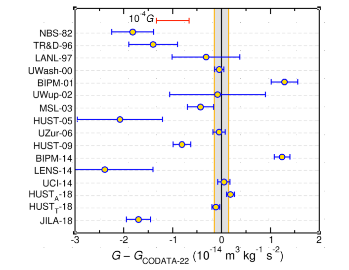
Figure 4: The 16 input data determining the Newtonian constant of gravitation $G$ ordered by publication year. The 2022 recommended value for $G$ has been subtracted. Error bars correspond to one-standard-deviation uncertainties as reported in Table 30. The uncertainties after applying the 3.9 multiplicative expansion factor to determine the 2022 recommended value are not shown. Labels on the left side of the figure denote the laboratories and the last two digits of the year in which the data were reported. See Table 30 for details. The gray band corresponds to the one-standard-deviation uncertainty of the recommended value.

Table 31: Observational equations for input data in Tables LABEL:tab:pdata and 27 as functions of the adjusted constants.

Input data		Observational equation		Sec.
D1	$a_{\rm e}({\rm exp})$	$\doteq$	$a_{\rm e}({\rm th})+\delta_{\rm th}({\rm e})$	V
D2	$\delta_{\rm e}$	$\doteq$	$\delta_{\rm th}({\rm e})$	V
D3, D4	$\displaystyle\frac{h}{m(X)}$	$\doteq$	$\displaystyle\frac{A_{\rm r}({\rm e})}{A_{\rm r}(X)}$ $\displaystyle\frac{c\alpha^{2}}{2R_{\infty}}$	VI
D5, D6	$A_{\rm r}(X)$	$\doteq$	$A_{\rm r}(X)$	II
D7	$\displaystyle\frac{\omega_{\rm s}(^{12}{\rm C}^{5+})}{\omega_{\rm c}(^{12}{\rm C}^{5+})}$	$\doteq$	$-\displaystyle\frac{g_{\rm e}(^{12}{\rm C}^{5+})+\delta_{\rm th}({\rm C})}{10A_{\rm r}({\rm e})}\left[12-5A_{\rm r}({\rm e})+\Delta E_{\rm B}(^{12}{\rm C}^{5+})\alpha^{2}A_{\rm r}({\rm e})/2R_{\infty}hc\right]$	VIII.3
D8, D12, D23, D24	$\Delta E_{\rm B}(X^{n+})$	$\doteq$	$\Delta E_{\rm B}(X^{n+})$	II
D9	$\delta_{\rm C}$	$\doteq$	$\delta_{\rm th}({\rm C})$	VIII.3
D10	$\displaystyle\frac{\omega_{\rm s}(^{28}{\rm Si}^{13+})}{\omega_{\rm c}(^{28}{\rm Si}^{13+})}$	$\doteq$	$-\displaystyle\frac{g_{\rm e}(^{28}{\rm Si}^{13+})+\delta_{\rm th}({\rm Si})}{26A_{\rm r}({\rm e})}A_{\rm r}(^{28}{\rm Si}^{13+})$	VIII.3
D11	$A_{\rm r}(^{28}{\rm Si})$	$\doteq$	$A_{\rm r}(^{28}{\rm Si}^{13+})+13A_{\rm r}({\rm e})-\Delta E_{\rm B}(^{28}{\rm Si^{13+}})\,\alpha^{2}A_{\rm r}({\rm e})/2R_{\infty}hc$	II
D13	$\delta_{\rm Si}$	$\doteq$	$\delta_{\rm th}({\rm Si})$	VIII.3
D14	$\eta_{\rm d}$	$\doteq$	$\displaystyle\frac{\alpha^{2}}{R_{\infty}}\,\displaystyle\frac{1}{d_{220}({\rm{\scriptstyle ILL}})}\,\displaystyle\frac{A_{\rm r}({\rm e})\,(A_{\rm r}({\rm n})+A_{\rm r}({\rm p}))}{(A_{\rm r}({\rm n})+A_{\rm r}({\rm p}))^{2}-A_{\rm r}({\rm d})^{2}}$	II
D15	$\displaystyle\frac{\omega_{\rm c}(^{12}{\rm C}^{6+})}{\omega_{\rm c}({\rm p})}$	$\doteq$	$\displaystyle\frac{6A_{\rm r}({\rm p})}{12-6A_{\rm r}({\rm e})+\Delta E_{\rm B}(^{12}{\rm C}^{6+})\,\alpha^{2}A_{\rm r}({\rm e})/2R_{\infty}hc}$	II
D16	$\displaystyle\frac{\omega_{\rm c}(^{12}{\rm C}^{6+})}{\omega_{\rm c}({\rm d})}$	$\doteq$	$\displaystyle\frac{6A_{\rm r}({\rm d})}{12-6A_{\rm r}({\rm e})+\Delta E_{\rm B}(^{12}{\rm C}^{6+})\,\alpha^{2}A_{\rm r}({\rm e})/2R_{\infty}hc}$	II
D17	$\displaystyle\frac{\omega_{\rm c}({\rm H}^{+}_{2})}{\omega_{\rm c}({\rm d})}$	$\doteq$	$\displaystyle\frac{A_{\rm r}({\rm d})}{2A_{\rm r}({\rm p})+A_{\rm r}({\rm e})-E_{\rm I}({\rm H}_{2}^{+})\,\alpha^{2}A_{\rm r}({\rm e})/2R_{\infty}hc}$	II
D18	$\displaystyle\frac{\omega_{\rm c}(^{12}{\rm C}^{4+})}{\omega_{\rm c}({\rm HD}^{+})}$	$\doteq$	$\displaystyle\frac{4[A_{\rm r}({\rm p})+A_{\rm r}({\rm d})+A_{\rm r}({\rm e})-\Delta E_{\rm I}({\rm HD^{+}})\,\alpha^{2}A_{\rm r}({\rm e})/2R_{\infty}hc]}{12-4A_{\rm r}({\rm e})+\Delta E_{\rm B}(^{12}{\rm C}^{4+})\,\alpha^{2}A_{\rm r}({\rm e})/2R_{\infty}hc}$	II
D19	$\displaystyle\frac{\omega_{\rm c}({\rm HD^{+}})}{\omega_{\rm c}(^{3}{\rm He}^{+})}$	$\doteq$	$\displaystyle\frac{A_{\rm r}({\rm h})+A_{\rm r}({\rm e})-E_{\rm I}(^{3}{\rm He^{+}})\,\alpha^{2}A_{\rm r}({\rm e})/2R_{\infty}hc}{A_{\rm r}({\rm p})+A_{\rm r}({\rm d})+A_{\rm r}({\rm e})-E_{\rm I}({\rm HD^{+}})\,\alpha^{2}A_{\rm r}({\rm e})/2R_{\infty}hc}$	II
D20	$\displaystyle\frac{\omega_{\rm c}({\rm t})}{\omega_{\rm c}(^{3}{\rm He}^{+})}$	$\doteq$	$\displaystyle\frac{A_{\rm r}({\rm h})+A_{\rm r}({\rm e})-E_{\rm I}(^{3}{\rm He^{+}})\,\alpha^{2}A_{\rm r}({\rm e})/2R_{\infty}hc}{A_{\rm r}({\rm t})}$	II
D21	$\displaystyle\frac{\omega_{\rm c}(^{4}{\rm He}^{2+})}{\omega_{\rm c}(^{12}{\rm C}^{6+})}$	$\doteq$	$\displaystyle\frac{12-6A_{\rm r}({\rm e})+\Delta E_{\rm B}(^{12}{\rm C}^{6+})\,\alpha^{2}A_{\rm r}({\rm e})/2R_{\infty}hc}{3A_{\rm r}(\mbox{{a}})}$	II
D22, D25, D26	$E_{\rm I}(X^{+})$	$\doteq$	$E_{\rm I}(X^{+})$	II
D27-D29	$f^{\rm exp}_{\rm SA}(vL\to v^{\prime}L^{\prime})$	$\doteq$	$f^{\rm th}_{\rm SA}(vL\to v^{\prime}L^{\prime})+\delta_{\rm HD^{+}}^{\rm th}(vL\to v^{\prime}L^{\prime})$	II.4
D30-D32	$\delta_{\rm HD^{+}}(vL\to v^{\prime}L^{\prime})$	$\doteq$	$\delta_{\rm HD^{+}}^{\rm th}(vL\to v^{\prime}L^{\prime})$	II.4
D33, D34	$R^{\prime}_{\mbox{\scriptsize{{{m}}}}}$	$\doteq$	$-\displaystyle\frac{a_{\mbox{\scriptsize{{{m}}}}}}{1+a_{\rm e}({\rm th})+\delta_{\rm th}({\rm e})}\displaystyle\frac{m_{\rm e}}{m_{\mbox{\scriptsize{{{m}}}}}}\displaystyle\frac{\mu_{\rm e}}{\mu^{\prime}_{\rm p}}$	VII.3
D35, D36	$E(\omega_{\rm p})$	$\doteq$	$E\!\left(\omega_{\rm p};R_{\infty},\alpha,\displaystyle\frac{m_{\rm e}}{m_{\mbox{\scriptsize{{{m}}}}}},a_{\mbox{\scriptsize{{{m}}}}},\displaystyle\frac{\mu_{\rm e}}{\mu_{\rm p}},\delta_{\rm th}({\rm e}),\delta_{\rm th}({\rm Mu})\right)$	IX.2
D37, D38	$\Delta E_{\rm Mu}$	$\doteq$	$\Delta E_{\rm Mu}\!\!\left({\rm th};R_{\infty},\alpha,\displaystyle\frac{m_{\rm e}}{m_{\mbox{\scriptsize{{{m}}}}}},a_{\mbox{\scriptsize{{{m}}}}}\right)+\delta_{\rm th}({\rm Mu})$	IX.1
D39	$\delta_{\rm Mu}$	$\doteq$	$\delta_{\rm th}({\rm Mu})$	IX.1
D40	$\displaystyle\frac{\mu_{\rm p}}{\mu_{\rm N}}$	$\doteq$	$-\left(1+a_{\rm e}({\rm th})+\delta_{\rm th}({\rm e})\right)\,\displaystyle\frac{A_{\rm r}({\rm p})}{A_{\rm r}({\rm e})}\,\displaystyle\frac{\mu_{\rm p}}{\mu_{\rm e}}$	XI.1
D41	$\displaystyle\frac{\mu_{\rm e}({\rm H})}{\mu_{\rm p}({\rm H})}$	$\doteq$	$\displaystyle\frac{g_{\rm e}({\rm H})}{g_{\rm e}}\left(\displaystyle\frac{g_{\rm p}({\rm H})}{g_{\rm p}}\right)^{-1}\displaystyle\frac{\mu_{\rm e}}{\mu_{\rm p}}$	X.4
D42	$\displaystyle\frac{\mu_{\rm d}({\rm D})}{\mu_{\rm e}({\rm D})}$	$\doteq$	$\displaystyle\frac{g_{\rm d}({\rm D})}{{g_{\rm d}}}\left(\displaystyle\frac{g_{\rm e}({\rm D})}{g_{\rm e}}\right)^{-1}\displaystyle\frac{\mu_{\rm d}}{\mu_{\rm e}}$	X.4
D43	$\displaystyle\frac{\mu_{\rm e}({\rm H})}{\mu_{\rm p}^{\prime}}$	$\doteq$	$\displaystyle\frac{g_{\rm e}({\rm H})}{g_{\rm e}}\displaystyle\frac{\mu_{\rm e}}{\mu_{\rm p}^{\prime}}$	X.4
D44	$\displaystyle\frac{\mu_{\rm h}(^{3}{\rm He})}{\mu_{\rm p}^{\prime}}$	$\doteq$	$\displaystyle\frac{\mu_{\rm h}(^{3}{\rm He})}{\mu_{\rm p}^{\prime}}$	X.4
D45	$\displaystyle\frac{\mu_{\rm h}(^{3}{\rm He^{+}})}{\mu_{\rm N}}$	$\doteq$	$-\displaystyle\frac{1-\sigma_{\rm h}(^{3}{\rm He^{+}})}{1-\sigma_{\rm h}(^{3}{\rm He})}\,\displaystyle\frac{\mu_{\rm h}(^{3}{\rm He})}{\mu_{\rm p}^{\prime}}\left(1+a_{\rm e}(\rm{th})+\delta_{\rm th}({\rm e})\right)\,\displaystyle\frac{A_{\rm r}({\rm p})}{A_{\rm r}(\rm e)}\,\displaystyle\frac{\mu_{\rm p}^{\prime}}{\mu_{\rm e}}$	XI.2
D46	$\displaystyle\frac{\mu_{\rm n}}{\mu_{\rm p}^{\prime}}$	$\doteq$	$\displaystyle\frac{\mu_{\rm n}}{\mu_{\rm p}^{\prime}}$	X.4
D47-D49	$\displaystyle\frac{\mu_{\rm p}({\rm HD})}{\mu_{\rm d}({\rm HD})}$	$\doteq$	$\left[1+\sigma_{\rm dp}\right]\displaystyle\frac{\mu_{\rm p}}{\mu_{\rm e}}\displaystyle\frac{\mu_{\rm e}}{\mu_{\rm d}}$	X.4
D50	$\displaystyle\frac{\mu_{\rm t}({\rm HT})}{\mu_{\rm p}({\rm HT})}$	$\doteq$	$\displaystyle\frac{1}{1+\sigma_{\rm tp}}\displaystyle\frac{\mu_{\rm t}}{\mu_{\rm p}}$	X.4
D51, D52	$\sigma_{NN^{\prime}}$	$\doteq$	$\sigma_{NN^{\prime}}$	X.3

XV The 2022 CODATA recommended values

XV.1 Calculational details

The focus of this section is the treatment of the data discussed in the previous sections to obtain the 2022 CODATA recommended values. In this regard, we recall that when the same expansion factor is applied to the a priori assigned uncertainties of both members of a correlated pair of input data to reduce data inconsistencies to an acceptable level, its square is also applied to their covariance so that their correlation coefficient is unchanged. For the same reason, when an expansion factor is only applied to the uncertainty of one member of a correlated pair, the expansion factor is applied to their covariance.

We begin with the 16 measurements of the Newtonian constant of gravitation $G$ in Table 30 and the three correlation coefficients in the table caption. As indicated in Sec. XIV, there have been no changes in or additions to these data since the 31 December 2018 closing date of the 2018 CODATA adjustment. Because $G$ is independent of all other constants, it can be determined in a separate least-squares adjustment, which is simply a calculation of their weighted mean. Since the data are unchanged, the same 3.9 expansion factor is used in this adjustment and the 2022 recommended value of $G$ is the same as the 2018 value.

The factor 3.9 reduces all normalized residuals to 2 or less, a long-established requirement of CODATA adjustments. For this adjustment, $\chi^{2}=12.9$, $p(12.9|15)=0.61$, and $R_{\rm B}=0.93$. (Here $p$ is the probability of $\chi^{2}=12.9$ for $\nu=N-M=16-1=15$ degrees of freedom occurring by chance and $R_{\rm B}=\sqrt{\chi^{2}/\nu}$ is the Birge ratio.) The two values of $G$ that had the largest residuals prior to expansion were BIPM-14 and JILA-18 in Table 30, which were $7.75$ and $-6.80$, respectively. In some past adjustments, input data with a self-sensitivity coefficient $S_{\rm c}$ less than $0.01$ were eliminated because they contributed less than 1 % to the determination of their own adjusted value. Although six of the sixteen values of $G$ have such small values of $S_{\rm c}$, they are retained because of the significant disagreements among the data and the desirability of having the recommended value reflect all of the data.

We next consider the silicon lattice spacing data in Table 27 with correlation coefficients in Table 28 and observational equations in Table 29. Because no new data of this type have become available in the past four years, like the $G$ data, they are the same as used in the 2018 adjustment. Also like the $G$ data, the silicon lattice spacing data were treated separately in the 2018 adjustment since they too were independent of all other input data. However, because there were no inconsistencies among them, no expansion factors were required.

The situation for silicon lattice spacings is somewhat different in the 2022 adjustment. As discussed in Sec. II.2, rather than using the 2020 AME value for $A_{\rm r}$(n), the TGFC decided to determine $A_{\rm r}$(n) from the original experimental data using Eq. (6) as the observational equation with the experimentally determined quantity $\eta_{\rm d}$ as the input datum. That equation not only contains the adjusted constant $A_{\rm r}$(n) but also the silicon lattice spacing adjusted constant $d_{220}$(ILL), which couples $\eta_{\rm d}$ to the lattice spacing data in Tables 27 and 28. Thus, in the 2022 adjustment, these data are not treated separately but are included as part of the calculation that uses all the input data except the $G$ data. However, because the adjusted constant $A_{\rm r}$(n) is not used in any other observational equation, the input datum $\eta_{\rm d}$ does not contribute to the determination of $d_{220}$(ILL) and hence the 2022 recommended values of the six silicon lattice spacing and x-ray related data given in Table XV.2 are identical to those in the corresponding Table XXXIII of the 2018 CODATA report Tiesinga et al. (2021a).

The following is a concise summary of the data that determine the 2022 CODATA recommended values other than $G$. For input data with correlation coefficients, their covariances are included in all calculations.

• Table 11, A1 to A29, H and D experimentally determined transition energies in kHz.

• Table 12, B1 to B25, additive energy corrections in kHz to the theoretical expressions for these transitions. The correlation coefficients for the data in these two tables are given in Table 13.

• Table LABEL:tab:muhdata, C1 to C6, muonic H, D, and ⁴He⁺ experimentally determined Lamb-shift transition energies in meV and additive energy corrections in meV to the theoretical expressions for these transitions. (The data in Table 15 are used in the theoretical expressions.)

• Table LABEL:tab:pdata, D1 to D52, a wide variety of input data ranging from the experimental value of the electron magnetic-moment anomaly $a_{\rm e}$(exp) to the theoretically calculated magnetic-shielding difference of the triton t and proton p in the HT molecule $\sigma_{\rm tp}$. The correlation coefficients among these 52 data are given in Table 26.

• Table 27, E1 to E21, experimentally determined lattice spacings, lattice spacing differences, and ratios of reference x-ray wave lengths to lattice spacings of a number of silicon crystals. The correlation coefficients among these 21 data are given in Table 28.

• Values of quantities the uncertainties of which are so small in the context in which they are used that they can be assumed to be exact. These include the reference constants in Table 2 and coefficients in Table 3 for the theoretical expressions for HD⁺ transition frequencies; Bethe logarithms in Table 5; theoretical values for various bound-particle to free-particle $g$-factor ratios in Table 24; and the magnetic shielding corrections $\sigma_{\rm h}(^{3}{\rm He})$ and $\sigma_{\rm h}(^{3}{\rm He}^{+})$ in Eqs. (201)-(203) and (215).

The 79 adjusted constants used in the observational equations for the 133 input data may be found in Tables 12 and 23 and the observational equations in Tables 29, 17, and 31. The degrees of freedom for adjustments with this dataset is $\nu=N-M=133-79=54$. For the initial least-squares adjustment without expansion factors, $\chi^{2}=109.6$, $p(109.6|54)=0.001\,\%$, and $R_{\rm B}=1.42$. This large value of $\chi^{2}$ is mainly due to the following eight input data, each with a normalized residual greater than 2: In Table 11, data A12 through A15 and A22 and A23, which are measured energy-level transitions in H and D; and in Table LABEL:tab:pdata, data D3 and D4, which are measurements of $h/m(^{87}{\rm Rb})$ and $h/m(^{133}{\rm Cs})$. The residuals of these eight data are 3.1, 2.5, 2.5, 3.1, 2.7, 3.4, $-$2.3, and 4.7, respectively.

The expansion factors of the uncertainties of the data to reduce these residuals to 2 or less are: (i) 1.7 for the 29 measured transition energies in Table 11 (A1 through A29) and the 25 additive corrections to the theoretical expressions for the transitions in Table 12 (B1 through B25); (ii) 1.7 for the six muonic H, D, and ⁴He⁺ Lamb-shift data in Table LABEL:tab:muhdata (C1 through C6); and (iii) 2.5 for the six data related to the determination of $\alpha$ at the beginning of Table LABEL:tab:pdata (D1 through D6). The expansion factor 1.7 is applied to the uncertainties of all the data in Tables 11 and 12 to maintain their original relative weights and correlations and is also applied to the six muonic atom Lamb-shift data for the same reason. Doing so ensures that all of the data that determine the Rydberg constant $R_{\infty}$ and the proton, deuteron, and alpha particle radii $r_{\rm p}$, $r_{\rm d}$, and $r_{\mbox{\scriptsize{{a}}}}$ contribute in the same proportion that they would have if no expansion factor was needed.

As expected, the final least-squares adjustment that determines the 2022 CODATA recommended values of the constants using the input data modified in this way yields the quite satisfactory results $\chi^{2}=44.2$, $p(44.2|54)=0.83$, and $R_{\rm B}=0.90$. As was the case for the 16 values of $G$ discussed above, a number of the 133 input data have self-sensitivity coefficients $S_{\rm c}$ less than 0.01. Nevertheless, they are retained for the same reason, namely because of the significant disagreements among some of the data and the desirability of having the recommended values reflect all of the relevant data.

XV.2 Tables of recommended values

The six tables 32 through 37, which have the same form as those in previous CODATA reports, give the 2022 recommended values of the basic constants and conversion factors of physics and chemistry and related quantities.

They range from Table 32, which gives an abbreviated list of constants, to Tables 36 and 37 which give energy equivalents. Although some of the 79 adjusted constants are recommended values, most are obtained from combinations of them taking into account their covariances. However, a few are based on the Particle Data Group values of the Fermi coupling constant $G_{\rm F}$, the weak mixing angle $\sin^{2}{\theta_{\rm w}}$, and the mass of the tau lepton Workman et al. (2022). The value of the free helion magnetic moment $\mu_{\rm h}$ is obtained from the adjusted constant $\mu_{\rm h}(^{3}{\rm He})/\mu^{\prime}_{\rm p}$ with the aid of the theoretically calculated value of the magnetic shielding constant $\mu_{\rm h}(^{3}{\rm He})/\mu_{\rm h}$ in Eq. (201) based on the expression $\mu_{\rm h}(^{3}{\rm He})=\mu_{\rm h}\left[1-\sigma_{\rm h}(^{3}{\rm He})\right]$.

All of the values given in these tables are available on the website of the Fundamental Constants Data Center of the NIST Physical Measurement Laboratory at physics.nist.gov/constants. In fact, like its predecessors, this electronic version of the 2022 CODATA recommended values of the constants enables users to obtain the correlation coefficient of any two constants listed in the tables. It also allows users to automatically convert the value of an energy-related quantity expressed in one unit to the corresponding value expressed in another unit (in essence, an automated version of Tables 36 and 37).

Table 32: An abbreviated list of the CODATA recommended values of the fundamental constants of physics and chemistry based on the 2022 adjustment.

				Relative std.
Quantity	Symbol	Value	Unit	uncert. $u_{\rm r}$
speed of light in vacuum	$c$	299 792 458	m s-1	exact
Newtonian constant of gravitation	$G$	$6.674\,30(15)\times 10^{-11}$	m3 kg-1 s-2	$2.2\times 10^{-5}$
Planck constant	$h$	$6.626\,070\,15\times 10^{-34}$	J Hz-1	exact
	$\hbar$	$1.054\,571\,817\ldots\times 10^{-34}$	J s	exact
elementary charge	$e$	$1.602\,176\,634\times 10^{-19}$	C	exact
vacuum magnetic permeability $4\mbox{{p}}\alpha\hbar/e^{2}c$	$\mu_{0}$	$1.256\,637\,061\,27(20)\times 10^{-6}$	N A-2	$1.6\times 10^{-10}$
vacuum electric permittivity 1/$\mu_{0}c^{2}$	$\epsilon_{0}$	$8.854\,187\,8188(14)\times 10^{-12}$	F m-1	$1.6\times 10^{-10}$
Josephson constant  2$e/h$	$K_{\rm J}$	$483\,597.848\,4\ldots\times 10^{9}$	Hz V-1	exact
von Klitzing constant $\mu_{0}c/2\alpha=2\mbox{{p}}\hbar/e^{2}$	$R_{\rm K}$	$25\,812.807\,45\ldots$	${\rm\Omega}$	exact
magnetic flux quantum $2\mbox{{p}}\hbar/(2e)$	${\it\Phi}_{0}$	$2.067\,833\,848\ldots\times 10^{-15}$	Wb	exact
conductance quantum $2e^{2}/2\mbox{{p}}\hbar$	$G_{0}$	$7.748\,091\,729\ldots\times 10^{-5}$	S	exact
electron mass	$m_{\rm e}$	$9.109\,383\,7139(28)\times 10^{-31}$	kg	$3.1\times 10^{-10}$
proton mass	$m_{\rm p}$	$1.672\,621\,925\,95(52)\times 10^{-27}$	kg	$3.1\times 10^{-10}$
proton-electron mass ratio	$m_{\rm p}$/$m_{\rm e}$	$1836.152\,673\,426(32)$		$1.7\times 10^{-11}$
fine-structure constant $e^{2}\!/4\mbox{{p}}\epsilon_{0}\hbar c$	$\alpha$	$7.297\,352\,5643(11)\times 10^{-3}$		$1.6\times 10^{-10}$
inverse fine-structure constant	$\alpha^{-1}$	$137.035\,999\,177(21)$		$1.6\times 10^{-10}$
Rydberg frequency $\alpha^{2}m_{\rm e}c^{2}/2h$	$cR_{\infty}$	$3.289\,841\,960\,2500(36)\times 10^{15}$	Hz	$1.1\times 10^{-12}$
Boltzmann constant	$k$	$1.380\,649\times 10^{-23}$	J K-1	exact
Avogadro constant	$N_{\rm A}$	$6.022\,140\,76\times 10^{23}$	mol-1	exact
molar gas constant $N_{\rm A}k$	$R$	$8.314\,462\,618\ldots$	J mol-1 K-1	exact
Faraday constant $N_{\rm A}e$	$F$	$96\,485.332\,12\ldots$	C mol-1	exact
Stefan-Boltzmann constant
($\mbox{{p}}^{2}$/60)$k^{4}\!/\hbar^{3}c^{2}$	$\sigma$	$5.670\,374\,419\ldots\times 10^{-8}$	W m-2 K-4	exact
Non-SI units accepted for use with the SI
electron volt ($e$/C) J	eV	$1.602\,176\,634\times 10^{-19}$	J	exact
(unified) atomic mass unit ${1\over 12}m(^{12}$C)	u	$1.660\,539\,068\,92(52)\times 10^{-27}$	kg	$3.1\times 10^{-10}$ —

Table 33: The CODATA recommended values of the fundamental constants of physics and chemistry based on the 2022 adjustment.

				Relative std.
Quantity	Symbol	Numerical value	Unit	uncert. $u_{\rm r}$
UNIVERSAL
speed of light in vacuum	$c$	$299\,792\,458$	m s-1	exact
vacuum magnetic permeability $4\mbox{{p}}\alpha\hbar/e^{2}c$	$\mu_{0}$	$1.256\,637\,061\,27(20)\times 10^{-6}$	N A-2	$1.6\times 10^{-10}$
$\mu_{0}/(4\mbox{{p}}\times 10^{-7})$		$0.999\,999\,999\,87(16)$	N A-2	$1.6\times 10^{-10}$
vacuum electric permittivity $1/\mu_{0}c^{2}$	$\epsilon_{0}$	$8.854\,187\,8188(14)\times 10^{-12}$	F m-1	$1.6\times 10^{-10}$
characteristic impedance of vacuum $\mu_{0}c$	$Z_{0}$	$376.730\,313\,412(59)$	${\rm\Omega}$	$1.6\times 10^{-10}$
Newtonian constant of gravitation	$G$	$6.674\,30(15)\times 10^{-11}$	m3 kg-1 s-2	$2.2\times 10^{-5}$
	$G/\hbar c$	$6.708\,83(15)\times 10^{-39}$	$({\rm GeV}/c^{2})^{-2}$	$2.2\times 10^{-5}$
Planck constant	$h$	$6.626\,070\,15\times 10^{-34}$	J Hz-1	exact
		$4.135\,667\,696\ldots\times 10^{-15}$	eV Hz-1	exact
	$\hbar$	$1.054\,571\,817\ldots\times 10^{-34}$	J s	exact
		$6.582\,119\,569\ldots\times 10^{-16}$	eV s	exact
	$\hbar c$	$197.326\,980\,4\ldots$	MeV fm	exact
Planck mass $(\hbar c/G)^{1/2}$	$m_{\rm P}$	$2.176\,434(24)\times 10^{-8}$	kg	$1.1\times 10^{-5}$
energy equivalent	$m_{\rm P}c^{2}$	$1.220\,890(14)\times 10^{19}$	GeV	$1.1\times 10^{-5}$
Planck temperature $(\hbar c^{5}/G)^{1/2}/k$	$T_{\rm P}$	$1.416\,784(16)\times 10^{32}$	K	$1.1\times 10^{-5}$
Planck length $\hbar/m_{\rm P}c=(\hbar G/c^{3})^{1/2}$	$l_{\rm P}$	$1.616\,255(18)\times 10^{-35}$	m	$1.1\times 10^{-5}$
Planck time $l_{\rm P}/c=(\hbar G/c^{5})^{1/2}$	$t_{\rm P}$	$5.391\,247(60)\times 10^{-44}$	s	$1.1\times 10^{-5}$
ELECTROMAGNETIC
elementary charge	$e$	$1.602\,176\,634\times 10^{-19}$	C	exact
	$e/\hbar$	$1.519\,267\,447\ldots\times 10^{15}$	A J-1	exact
magnetic flux quantum $2\mbox{{p}}\hbar/(2e)$	${\it\Phi}_{0}$	$2.067\,833\,848\ldots\times 10^{-15}$	Wb	exact
conductance quantum $2e^{2}\!/2\mbox{{p}}\hbar$	$G_{0}$	$7.748\,091\,729\ldots\times 10^{-5}$	S	exact
inverse of conductance quantum	$G_{0}^{-1}$	$12\,906.403\,72\ldots$	${\rm\Omega}$	exact
Josephson constant  2$e/h$	$K_{\rm J}$	$483\,597.848\,4\ldots\times 10^{9}$	Hz V-1	exact
von Klitzing constant $\mu_{0}c/2\alpha=2\mbox{{p}}\hbar/e^{2}$	$R_{\rm K}$	$25\,812.807\,45\ldots$	${\rm\Omega}$	exact
Bohr magneton $e\hbar/2m_{\rm e}$	$\mu_{\rm B}$	$9.274\,010\,0657(29)\times 10^{-24}$	J T-1	$3.1\times 10^{-10}$
		$5.788\,381\,7982(18)\times 10^{-5}$	eV T-1	$3.1\times 10^{-10}$
	$\mu_{\rm B}/h$	$1.399\,624\,491\,71(44)\times 10^{10}$	Hz T-1	$3.1\times 10^{-10}$
	$\mu_{\rm B}/hc$	$46.686\,447\,719(15)$	[m${}^{-1}~{}$T-1]a	$3.1\times 10^{-10}$
	$\mu_{\rm B}/k$	$0.671\,713\,814\,72(21)$	K T-1	$3.1\times 10^{-10}$
nuclear magneton $e\hbar/2m_{\rm p}$	$\mu_{\rm N}$	$5.050\,783\,7393(16)\times 10^{-27}$	J T-1	$3.1\times 10^{-10}$
		$3.152\,451\,254\,17(98)\times 10^{-8}$	eV T-1	$3.1\times 10^{-10}$
	$\mu_{\rm N}/h$	$7.622\,593\,2188(24)$	MHz T-1	$3.1\times 10^{-10}$
	$\mu_{\rm N}/hc$	$2.542\,623\,410\,09(79)\times 10^{-2}$	[m${}^{-1}~{}$T-1]a	$3.1\times 10^{-10}$
	$\mu_{\rm N}/k$	$3.658\,267\,7706(11)\times 10^{-4}$	K T-1	$3.1\times 10^{-10}$
ATOMIC AND NUCLEAR
General
fine-structure constant $e^{2}\!/4\mbox{{p}}\epsilon_{0}\hbar c$	$\alpha$	$7.297\,352\,5643(11)\times 10^{-3}$		$1.6\times 10^{-10}$
inverse fine-structure constant	$\alpha^{-1}$	$137.035\,999\,177(21)$		$1.6\times 10^{-10}$
Rydberg frequency $\alpha^{2}m_{\rm e}c^{2}/2h=E_{\rm h}/2h$	$cR_{\infty}$	$3.289\,841\,960\,2500(36)\times 10^{15}$	Hz	$1.1\times 10^{-12}$
energy equivalent	$hc\,R_{\infty}$	$2.179\,872\,361\,1030(24)\times 10^{-18}$	J	$1.1\times 10^{-12}$
		$13.605\,693\,122\,990(15)$	eV	$1.1\times 10^{-12}$
Rydberg constant	$R_{\infty}$	$10\,973\,731.568\,157(12)$	[m-1]a	$1.1\times 10^{-12}$
Bohr radius ${\hbar/\alpha m_{\rm e}c}=4\mbox{{p}}\epsilon_{0}\hbar^{2}\!/m_{\rm e}e^{2}$	$a_{\rm 0}$	$5.291\,772\,105\,44(82)\times 10^{-11}$	m	$1.6\times 10^{-10}$
Hartree energy $\alpha^{2}m_{\rm e}c^{2}=e^{2}\!/4\mbox{{p}}\epsilon_{\rm 0}a_{\rm 0}=2hcR_{\infty}$	$E_{\rm h}$	$4.359\,744\,722\,2060(48)\times 10^{-18}$	J	$1.1\times 10^{-12}$
		$27.211\,386\,245\,981(30)$	eV	$1.1\times 10^{-12}$
quantum of circulation	$\mbox{{p}}\hbar/m_{\rm e}$	$3.636\,947\,5467(11)\times 10^{-4}$	m${}^{2}~{}$s-1	$3.1\times 10^{-10}$
	$2\mbox{{p}}\hbar/m_{\rm e}$	$7.273\,895\,0934(23)\times 10^{-4}$	m${}^{2}~{}$s-1	$3.1\times 10^{-10}$
Electroweak
Fermi coupling constantb	$G_{\rm F}/(\hbar c)^{3}$	$1.166\,3787(6)\times 10^{-5}$	GeV-2	$5.1\times 10^{-7}$
weak mixing anglec $\theta_{\rm W}$ (on-shell scheme)
$\sin^{2}\theta_{\rm W}=s^{2}_{\rm W}\equiv 1-(m_{\rm W}/m_{\rm Z})^{2}$	$\sin^{2}\theta_{\rm W}$	$0.223\,05(23)$		$1.0\times 10^{-3}$
Electron, e-
electron mass	$m_{\rm e}$	$9.109\,383\,7139(28)\times 10^{-31}$	kg	$3.1\times 10^{-10}$
		$5.485\,799\,090\,441(97)\times 10^{-4}$	u	$1.8\times 10^{-11}$
energy equivalent	$m_{\rm e}c^{2}$	$8.187\,105\,7880(26)\times 10^{-14}$	J	$3.1\times 10^{-10}$
		$0.510\,998\,950\,69(16)$	MeV	$3.1\times 10^{-10}$
electron-muon mass ratio	$m_{\rm e}/m_{\mbox{\scriptsize{{{m}}}}}$	$4.836\,331\,70(11)\times 10^{-3}$		$2.2\times 10^{-8}$
electron-tau mass ratio	$m_{\rm e}/m_{\mbox{\scriptsize{{t}}}}$	$2.875\,85(19)\times 10^{-4}$		$6.8\times 10^{-5}$
electron-proton mass ratio	$m_{\rm e}/m_{\rm p}$	$5.446\,170\,214\,889(94)\times 10^{-4}$		$1.7\times 10^{-11}$
electron-neutron mass ratio	$m_{\rm e}/m_{\rm n}$	$5.438\,673\,4416(22)\times 10^{-4}$		$4.0\times 10^{-10}$
electron-deuteron mass ratio	$m_{\rm e}/m_{\rm d}$	$2.724\,437\,107\,629(47)\times 10^{-4}$		$1.7\times 10^{-11}$
electron-triton mass ratio	$m_{\rm e}/m_{\rm t}$	$1.819\,200\,062\,327(68)\times 10^{-4}$		$3.8\times 10^{-11}$
electron-helion mass ratio	$m_{\rm e}/m_{\rm h}$	$1.819\,543\,074\,649(53)\times 10^{-4}$		$2.9\times 10^{-11}$
electron to alpha particle mass ratio	$m_{\rm e}/m_{\mbox{\scriptsize{{a}}}}$	$1.370\,933\,554\,733(32)\times 10^{-4}$		$2.4\times 10^{-11}$
electron charge to mass quotient	$-e/m_{\rm e}$	$-1.758\,820\,008\,38(55)\times 10^{11}$	C kg-1	$3.1\times 10^{-10}$
electron molar mass $N_{\rm A}m_{\rm e}$	$M({\rm e}),M_{\rm e}$	$5.485\,799\,0962(17)\times 10^{-7}$	kg mol-1	$3.1\times 10^{-10}$
reduced Compton wavelength $\hbar/m_{\rm e}c=\alpha a_{0}$	$\lambda\hskip-4.5pt\vrule height=4.6pt,depth=-4.3pt,width=4.0pt_{\rm C}$	$3.861\,592\,6744(12)\times 10^{-13}$	m	$3.1\times 10^{-10}$
Compton wavelength	$\lambda_{\rm C}$	$2.426\,310\,235\,38(76)\times 10^{-12}$	[m]a	$3.1\times 10^{-10}$
classical electron radius $\alpha^{2}a_{\rm 0}$	$r_{\rm e}$	$2.817\,940\,3205(13)\times 10^{-15}$	m	$4.7\times 10^{-10}$
Thomson cross section (8$\mbox{{p}}/3)r^{2}_{\rm e}$	$\sigma_{\rm e}$	$6.652\,458\,7051(62)\times 10^{-29}$	m2	$9.3\times 10^{-10}$
electron magnetic moment	$\mu_{\rm e}$	$-9.284\,764\,6917(29)\times 10^{-24}$	J T-1	$3.1\times 10^{-10}$
to Bohr magneton ratio	$\mu_{\rm e}/\mu_{\rm B}$	$-1.001\,159\,652\,180\,46(18)$		$1.8\times 10^{-13}$
to nuclear magneton ratio	$\mu_{\rm e}/\mu_{\rm N}$	$-1838.281\,971\,877(32)$		$1.7\times 10^{-11}$
electron magnetic-moment
anomaly $|\mu_{\rm e}|/\mu_{\rm B}-1$	$a_{\rm e}$	$1.159\,652\,180\,46(18)\times 10^{-3}$		$1.6\times 10^{-10}$
electron $g$-factor $-2(1+a_{\rm e})$	$g_{\rm e}$	$-2.002\,319\,304\,360\,92(36)$		$1.8\times 10^{-13}$
electron-muon magnetic-moment ratio	$\mu_{\rm e}/\mu_{\mbox{\scriptsize{{{m}}}}}$	$206.766\,9881(46)$		$2.2\times 10^{-8}$
electron-proton magnetic-moment ratio	$\mu_{\rm e}/\mu_{\rm p}$	$-658.210\,687\,89(19)$		$3.0\times 10^{-10}$
electron to shielded proton magnetic-
moment ratio (H2O, sphere, 25 ∘C)	$\mu_{\rm e}/\mu^{\prime}_{\rm p}$	$-658.227\,5856(27)$		$4.1\times 10^{-9}$
electron-neutron magnetic-moment ratio	$\mu_{\rm e}/\mu_{\rm n}$	$960.920\,48(23)$		$2.4\times 10^{-7}$
electron-deuteron magnetic-moment ratio	$\mu_{\rm e}/\mu_{\rm d}$	$-2143.923\,4921(56)$		$2.6\times 10^{-9}$
electron to bound helion magnetic-
moment ratio	$\mu_{\rm e}/\mu_{\rm h}(^{3}{\rm He})$	$864.058\,239\,86(70)$		$8.1\times 10^{-10}$
electron gyromagnetic ratio $2|\mu_{\rm e}|/\hbar$	$\gamma_{\rm e}$	$1.760\,859\,627\,84(55)\times 10^{11}$	s${}^{-1}~{}$T-1	$3.1\times 10^{-10}$
		$28\,024.951\,3861(87)$	MHz T-1	$3.1\times 10^{-10}$
Muon, ${\mbox{{m}}}^{-}$
muon mass	$m_{\mbox{\scriptsize{{{m}}}}}$	$1.883\,531\,627(42)\times 10^{-28}$	kg	$2.2\times 10^{-8}$
		$0.113\,428\,9257(25)$	u	$2.2\times 10^{-8}$
energy equivalent	$m_{\mbox{\scriptsize{{{m}}}}}c^{2}$	$1.692\,833\,804(38)\times 10^{-11}$	J	$2.2\times 10^{-8}$
		$105.658\,3755(23)$	MeV	$2.2\times 10^{-8}$
muon-electron mass ratio	$m_{\mbox{\scriptsize{{{m}}}}}/m_{\rm e}$	$206.768\,2827(46)$		$2.2\times 10^{-8}$
muon-tau mass ratio	$m_{\mbox{\scriptsize{{{m}}}}}/m_{\mbox{\scriptsize{{t}}}}$	$5.946\,35(40)\times 10^{-2}$		$6.8\times 10^{-5}$
muon-proton mass ratio	$m_{\mbox{\scriptsize{{{m}}}}}/m_{\rm p}$	$0.112\,609\,5262(25)$		$2.2\times 10^{-8}$
muon-neutron mass ratio	$m_{\mbox{\scriptsize{{{m}}}}}/m_{\rm n}$	$0.112\,454\,5168(25)$		$2.2\times 10^{-8}$
muon molar mass $N_{\rm A}m_{\mbox{\scriptsize{{{m}}}}}$	$M({\mbox{{m}}}),M_{\mbox{\scriptsize{{{m}}}}}$	$1.134\,289\,258(25)\times 10^{-4}$	kg mol-1	$2.2\times 10^{-8}$
reduced muon Compton wavelength $\hbar/m_{\mbox{\scriptsize{{{m}}}}}c$	$\lambda\hskip-4.5pt\vrule height=4.6pt,depth=-4.3pt,width=4.0pt_{{\rm C},{\mbox{\scriptsize{{{m}}}}}}$	$1.867\,594\,306(42)\times 10^{-15}$	m	$2.2\times 10^{-8}$
muon Compton wavelength	$\lambda_{{\rm C},{\mbox{\scriptsize{{{m}}}}}}$	$1.173\,444\,110(26)\times 10^{-14}$	[m]a	$2.2\times 10^{-8}$
muon magnetic moment	$\mu_{\mbox{\scriptsize{{{m}}}}}$	$-4.490\,448\,30(10)\times 10^{-26}$	J T-1	$2.2\times 10^{-8}$
to Bohr magneton ratio	$\mu_{\mbox{\scriptsize{{{m}}}}}/\mu_{\rm B}$	$-4.841\,970\,48(11)\times 10^{-3}$		$2.2\times 10^{-8}$
to nuclear magneton ratio	$\mu_{\mbox{\scriptsize{{{m}}}}}/\mu_{\rm N}$	$-8.890\,597\,04(20)$		$2.2\times 10^{-8}$
muon magnetic-moment anomaly
$|\mu_{\mbox{\scriptsize{{{m}}}}}|/(e\hbar/2m_{\mbox{\scriptsize{{{m}}}}})-1$	$a_{\mbox{\scriptsize{{{m}}}}}$	$1.165\,920\,62(41)\times 10^{-3}$		$3.5\times 10^{-7}$
muon $g$-factor $-2(1+a_{\mbox{\scriptsize{{{m}}}}}$)	$g_{\mbox{\scriptsize{{{m}}}}}$	$-2.002\,331\,841\,23(82)$		$4.1\times 10^{-10}$
muon-proton magnetic-moment ratio	$\mu_{\mbox{\scriptsize{{{m}}}}}/\mu_{\rm p}$	$-3.183\,345\,146(71)$		$2.2\times 10^{-8}$
Tau, ${\mbox{{t}}}^{-}$
tau massd	$m_{\mbox{\scriptsize{{t}}}}$	$3.167\,54(21)\times 10^{-27}$	kg	$6.8\times 10^{-5}$
		$1.907\,54(13)$	u	$6.8\times 10^{-5}$
energy equivalent	$m_{\mbox{\scriptsize{{t}}}}c^{2}$	$2.846\,84(19)\times 10^{-10}$	J	$6.8\times 10^{-5}$
		$1776.86(12)$	MeV	$6.8\times 10^{-5}$
tau-electron mass ratio	$m_{\mbox{\scriptsize{{t}}}}/m_{\rm e}$	$3477.23(23)$		$6.8\times 10^{-5}$
tau-muon mass ratio	$m_{\mbox{\scriptsize{{t}}}}/m_{\mbox{\scriptsize{{{m}}}}}$	$16.8170(11)$		$6.8\times 10^{-5}$
tau-proton mass ratio	$m_{\mbox{\scriptsize{{t}}}}/m_{\rm p}$	$1.893\,76(13)$		$6.8\times 10^{-5}$
tau-neutron mass ratio	$m_{\mbox{\scriptsize{{t}}}}/m_{\rm n}$	$1.891\,15(13)$		$6.8\times 10^{-5}$
tau molar mass $N_{\rm A}m_{\mbox{\scriptsize{{t}}}}$	$M({\mbox{{t}}}),M_{\mbox{\scriptsize{{t}}}}$	$1.907\,54(13)\times 10^{-3}$	kg mol-1	$6.8\times 10^{-5}$
reduced tau Compton wavelength $\hbar/m_{\mbox{\scriptsize{{t}}}}c$	$\lambda\hskip-4.5pt\vrule height=4.6pt,depth=-4.3pt,width=4.0pt_{{\rm C},{\mbox{\scriptsize{{t}}}}}$	$1.110\,538(75)\times 10^{-16}$	m	$6.8\times 10^{-5}$
tau Compton wavelength	$\lambda_{{\rm C},{\mbox{\scriptsize{{t}}}}}$	$6.977\,71(47)\times 10^{-16}$	[m]a	$6.8\times 10^{-5}$
Proton, p
proton mass	$m_{\rm p}$	$1.672\,621\,925\,95(52)\times 10^{-27}$	kg	$3.1\times 10^{-10}$
		$1.007\,276\,466\,5789(83)$	u	$8.3\times 10^{-12}$
energy equivalent	$m_{\rm p}c^{2}$	$1.503\,277\,618\,02(47)\times 10^{-10}$	J	$3.1\times 10^{-10}$
		$938.272\,089\,43(29)$	MeV	$3.1\times 10^{-10}$
proton-electron mass ratio	$m_{\rm p}/m_{\rm e}$	$1836.152\,673\,426(32)$		$1.7\times 10^{-11}$
proton-muon mass ratio	$m_{\rm p}/m_{\mbox{\scriptsize{{{m}}}}}$	$8.880\,243\,38(20)$		$2.2\times 10^{-8}$
proton-tau mass ratio	$m_{\rm p}/m_{\mbox{\scriptsize{{t}}}}$	$0.528\,051(36)$		$6.8\times 10^{-5}$
proton-neutron mass ratio	$m_{\rm p}/m_{\rm n}$	$0.998\,623\,477\,97(40)$		$4.0\times 10^{-10}$
proton charge to mass quotient	$e/m_{\rm p}$	$9.578\,833\,1430(30)\times 10^{7}$	C kg-1	$3.1\times 10^{-10}$
proton molar mass $N_{\rm A}m_{\rm p}$	$M$(p), $M_{\rm p}$	$1.007\,276\,467\,64(31)\times 10^{-3}$	kg mol-1	$3.1\times 10^{-10}$
reduced proton Compton wavelength $\hbar/m_{\rm p}c$	$\lambda\hskip-4.5pt\vrule height=4.6pt,depth=-4.3pt,width=4.0pt_{\rm C,p}$	$2.103\,089\,100\,51(66)\times 10^{-16}$	m	$3.1\times 10^{-10}$
proton Compton wavelength	$\lambda_{\rm C,p}$	$1.321\,409\,853\,60(41)\times 10^{-15}$	[m]a	$3.1\times 10^{-10}$
proton rms charge radius	$r_{\rm p}$	$8.4075(64)\times 10^{-16}$	m	$7.6\times 10^{-4}$
proton magnetic moment	$\mu_{\rm p}$	$1.410\,606\,795\,45(60)\times 10^{-26}$	J T-1	$4.3\times 10^{-10}$
to Bohr magneton ratio	$\mu_{\rm p}/\mu_{\rm B}$	$1.521\,032\,202\,30(45)\times 10^{-3}$		$3.0\times 10^{-10}$
to nuclear magneton ratio	$\mu_{\rm p}/\mu_{\rm N}$	$2.792\,847\,344\,63(82)$		$2.9\times 10^{-10}$
proton $g$-factor $2\mu_{\rm p}/\mu_{\rm N}$	$g_{\rm p}$	$5.585\,694\,6893(16)$		$2.9\times 10^{-10}$
proton-neutron magnetic-moment ratio	$\mu_{\rm p}/\mu_{\rm n}$	$-1.459\,898\,02(34)$		$2.4\times 10^{-7}$
shielded proton magnetic moment
(H2O, sphere, 25 ∘C)	$\mu^{\prime}_{\rm p}$	$1.410\,570\,5830(58)\times 10^{-26}$	J T-1	$4.1\times 10^{-9}$
to Bohr magneton ratio	$\mu^{\prime}_{\rm p}/\mu_{\rm B}$	$1.520\,993\,1551(62)\times 10^{-3}$		$4.1\times 10^{-9}$
to nuclear magneton ratio	$\mu^{\prime}_{\rm p}/\mu_{\rm N}$	$2.792\,775\,648(11)$		$4.1\times 10^{-9}$
proton magnetic shielding correction
$1-\mu^{\prime}_{\rm p}/\mu_{\rm p}$  (H2O, sphere, 25 ∘C)	$\sigma^{\prime}_{\rm p}$	$2.567\,15(41)\times 10^{-5}$		$1.6\times 10^{-4}$
proton gyromagnetic ratio $2\mu_{\rm p}/\hbar$	$\gamma_{\rm p}$	$2.675\,221\,8708(11)\times 10^{8}$	s${}^{-1}~{}$T-1	$4.3\times 10^{-10}$
		$42.577\,478\,461(18)$	MHz T-1	$4.3\times 10^{-10}$
shielded proton gyromagnetic ratio
$2\mu^{\prime}_{\rm p}/\hbar$  (H2O, sphere, 25 ∘C)	$\gamma^{\prime}_{\rm p}$	$2.675\,153\,194(11)\times 10^{8}$	s${}^{-1}~{}$T-1	$4.1\times 10^{-9}$
		$42.576\,385\,43(17)$	MHz T-1	$4.1\times 10^{-9}$
Neutron, n
neutron mass	$m_{\rm n}$	$1.674\,927\,500\,56(85)\times 10^{-27}$	kg	$5.1\times 10^{-10}$
		$1.008\,664\,916\,06(40)$	u	$4.0\times 10^{-10}$
energy equivalent	$m_{\rm n}c^{2}$	$1.505\,349\,765\,14(76)\times 10^{-10}$	J	$5.1\times 10^{-10}$
		$939.565\,421\,94(48)$	MeV	$5.1\times 10^{-10}$
neutron-electron mass ratio	$m_{\rm n}/m_{\rm e}$	$1838.683\,662\,00(74)$		$4.0\times 10^{-10}$
neutron-muon mass ratio	$m_{\rm n}/m_{\mbox{\scriptsize{{{m}}}}}$	$8.892\,484\,08(20)$		$2.2\times 10^{-8}$
neutron-tau mass ratio	$m_{\rm n}/m_{\mbox{\scriptsize{{t}}}}$	$0.528\,779(36)$		$6.8\times 10^{-5}$
neutron-proton mass ratio	$m_{\rm n}/m_{\rm p}$	$1.001\,378\,419\,46(40)$		$4.0\times 10^{-10}$
neutron-proton mass difference	$m_{\rm n}-m_{\rm p}$	$2.305\,574\,61(67)\times 10^{-30}$	kg	$2.9\times 10^{-7}$
		$1.388\,449\,48(40)\times 10^{-3}$	u	$2.9\times 10^{-7}$
energy equivalent	($m_{\rm n}-m_{\rm p})c^{2}$	$2.072\,147\,12(60)\times 10^{-13}$	J	$2.9\times 10^{-7}$
		$1.293\,332\,51(38)$	MeV	$2.9\times 10^{-7}$
neutron molar mass $N_{\rm A}m_{\rm n}$	$M({\rm n}),M_{\rm n}$	$1.008\,664\,917\,12(51)\times 10^{-3}$	kg mol-1	$5.1\times 10^{-10}$
reduced neutron Compton wavelength $\hbar/m_{\rm n}c$	$\lambda\hskip-4.5pt\vrule height=4.6pt,depth=-4.3pt,width=4.0pt_{\rm C,n}$	$2.100\,194\,1520(11)\times 10^{-16}$	m	$5.1\times 10^{-10}$
neutron Compton wavelength	$\lambda_{\rm C,n}$	$1.319\,590\,903\,82(67)\times 10^{-15}$	[m]a	$5.1\times 10^{-10}$
neutron magnetic moment	$\mu_{\rm n}$	$-9.662\,3653(23)\times 10^{-27}$	J T-1	$2.4\times 10^{-7}$
to Bohr magneton ratio	$\mu_{\rm n}/\mu_{\rm B}$	$-1.041\,875\,65(25)\times 10^{-3}$		$2.4\times 10^{-7}$
to nuclear magneton ratio	$\mu_{\rm n}/\mu_{\rm N}$	$-1.913\,042\,76(45)$		$2.4\times 10^{-7}$
neutron $g$-factor $2\mu_{\rm n}/\mu_{\rm N}$	$g_{\rm n}$	$-3.826\,085\,52(90)$		$2.4\times 10^{-7}$
neutron-electron magnetic-moment ratio	$\mu_{\rm n}/\mu_{\rm e}$	$1.040\,668\,84(24)\times 10^{-3}$		$2.4\times 10^{-7}$
neutron-proton magnetic-moment ratio	$\mu_{\rm n}/\mu_{\rm p}$	$-0.684\,979\,35(16)$		$2.4\times 10^{-7}$
neutron to shielded proton magnetic-
moment ratio  (H2O, sphere, 25 ∘C)	$\mu_{\rm n}/\mu_{\rm p}^{\prime}$	$-0.684\,996\,94(16)$		$2.4\times 10^{-7}$
neutron gyromagnetic ratio $2|\mu_{\rm n}|/\hbar$	$\gamma_{\rm n}$	$1.832\,471\,74(43)\times 10^{8}$	s${}^{-1}~{}$T-1	$2.4\times 10^{-7}$
		$29.164\,6935(69)$	MHz T-1	$2.4\times 10^{-7}$
Deuteron, d
deuteron mass	$m_{\rm d}$	$3.343\,583\,7768(10)\times 10^{-27}$	kg	$3.1\times 10^{-10}$
		$2.013\,553\,212\,544(15)$	u	$7.4\times 10^{-12}$
energy equivalent	$m_{\rm d}c^{2}$	$3.005\,063\,234\,91(94)\times 10^{-10}$	J	$3.1\times 10^{-10}$
		$1875.612\,945\,00(58)$	MeV	$3.1\times 10^{-10}$
deuteron-electron mass ratio	$m_{\rm d}/m_{\rm e}$	$3670.482\,967\,655(63)$		$1.7\times 10^{-11}$
deuteron-proton mass ratio	$m_{\rm d}/m_{\rm p}$	$1.999\,007\,501\,2699(84)$		$4.2\times 10^{-12}$
deuteron molar mass $N_{\rm A}m_{\rm d}$	$M({\rm d}),M_{\rm d}$	$2.013\,553\,214\,66(63)\times 10^{-3}$	kg mol-1	$3.1\times 10^{-10}$
deuteron rms charge radius	$r_{\rm d}$	$2.127\,78(27)\times 10^{-15}$	m	$1.3\times 10^{-4}$
deuteron magnetic moment	$\mu_{\rm d}$	$4.330\,735\,087(11)\times 10^{-27}$	J T-1	$2.6\times 10^{-9}$
to Bohr magneton ratio	$\mu_{\rm d}/\mu_{\rm B}$	$4.669\,754\,568(12)\times 10^{-4}$		$2.6\times 10^{-9}$
to nuclear magneton ratio	$\mu_{\rm d}/\mu_{\rm N}$	$0.857\,438\,2335(22)$		$2.6\times 10^{-9}$
deuteron $g$-factor $\mu_{\rm d}/\mu_{\rm N}$	$g_{\rm d}$	$0.857\,438\,2335(22)$		$2.6\times 10^{-9}$
deuteron-electron magnetic-moment ratio	$\mu_{\rm d}/\mu_{\rm e}$	$-4.664\,345\,550(12)\times 10^{-4}$		$2.6\times 10^{-9}$
deuteron-proton magnetic-moment ratio	$\mu_{\rm d}/\mu_{\rm p}$	$0.307\,012\,209\,30(79)$		$2.6\times 10^{-9}$
deuteron-neutron magnetic-moment ratio	$\mu_{\rm d}/\mu_{\rm n}$	$-0.448\,206\,52(11)$		$2.4\times 10^{-7}$
Triton, t
triton mass	$m_{\rm t}$	$5.007\,356\,7512(16)\times 10^{-27}$	kg	$3.1\times 10^{-10}$
		$3.015\,500\,715\,97(10)$	u	$3.4\times 10^{-11}$
energy equivalent	$m_{\rm t}c^{2}$	$4.500\,387\,8119(14)\times 10^{-10}$	J	$3.1\times 10^{-10}$
		$2808.921\,136\,68(88)$	MeV	$3.1\times 10^{-10}$
triton-electron mass ratio	$m_{\rm t}/m_{\rm e}$	$5496.921\,535\,51(21)$		$3.8\times 10^{-11}$
triton-proton mass ratio	$m_{\rm t}/m_{\rm p}$	$2.993\,717\,034\,03(10)$		$3.4\times 10^{-11}$
triton molar mass $N_{\rm A}m_{\rm t}$	$M({\rm t}),M_{\rm t}$	$3.015\,500\,719\,13(94)\times 10^{-3}$	kg mol-1	$3.1\times 10^{-10}$
triton magnetic moment	$\mu_{\rm t}$	$1.504\,609\,5178(30)\times 10^{-26}$	J T-1	$2.0\times 10^{-9}$
to Bohr magneton ratio	$\mu_{\rm t}/\mu_{\rm B}$	$1.622\,393\,6648(32)\times 10^{-3}$		$2.0\times 10^{-9}$
to nuclear magneton ratio	$\mu_{\rm t}/\mu_{\rm N}$	$2.978\,962\,4650(59)$		$2.0\times 10^{-9}$
triton $g$-factor $2\mu_{\rm t}/\mu_{\rm N}$	$g_{\rm t}$	$5.957\,924\,930(12)$		$2.0\times 10^{-9}$
Helion, h
helion mass	$m_{\rm h}$	$5.006\,412\,7862(16)\times 10^{-27}$	kg	$3.1\times 10^{-10}$
		$3.014\,932\,246\,932(74)$	u	$2.5\times 10^{-11}$
energy equivalent	$m_{\rm h}c^{2}$	$4.499\,539\,4185(14)\times 10^{-10}$	J	$3.1\times 10^{-10}$
		$2808.391\,611\,12(88)$	MeV	$3.1\times 10^{-10}$
helion-electron mass ratio	$m_{\rm h}/m_{\rm e}$	$5495.885\,279\,84(16)$		$2.9\times 10^{-11}$
helion-proton mass ratio	$m_{\rm h}/m_{\rm p}$	$2.993\,152\,671\,552(70)$		$2.4\times 10^{-11}$
helion molar mass $N_{\rm A}m_{\rm h}$	$M({\rm h}),M_{\rm h}$	$3.014\,932\,250\,10(94)\times 10^{-3}$	kg mol-1	$3.1\times 10^{-10}$
helion magnetic moment	$\mu_{\rm h}$	$-1.074\,617\,551\,98(93)\times 10^{-26}$	J T-1	$8.7\times 10^{-10}$
to Bohr magneton ratio	$\mu_{\rm h}/\mu_{\rm B}$	$-1.158\,740\,980\,83(94)\times 10^{-3}$		$8.1\times 10^{-10}$
to nuclear magneton ratio	$\mu_{\rm h}/\mu_{\rm N}$	$-2.127\,625\,3498(17)$		$8.1\times 10^{-10}$
helion $g$-factor $2\mu_{\rm h}/\mu_{\rm N}$	$g_{\rm h}$	$-4.255\,250\,6995(34)$		$8.1\times 10^{-10}$
bound helion magnetic moment	$\mu_{\rm h}(^{3}{\rm He})$	$-1.074\,553\,110\,35(93)\times 10^{-26}$	J T-1	$8.7\times 10^{-10}$
to Bohr magneton ratio	$\mu_{\rm h}(^{3}{\rm He})/\mu_{\rm B}$	$-1.158\,671\,494\,57(94)\times 10^{-3}$		$8.1\times 10^{-10}$
to nuclear magneton ratio	$\mu_{\rm h}(^{3}{\rm He})/\mu_{\rm N}$	$-2.127\,497\,7624(17)$		$8.1\times 10^{-10}$
bound helion to proton magnetic-
moment ratio	$\mu_{\rm h}(^{3}{\rm He})/\mu_{\rm p}$	$-0.761\,766\,577\,21(66)$		$8.6\times 10^{-10}$
bound helion to shielded proton magnetic-
moment ratio  (H2O, sphere, 25 ∘C)	$\mu_{\rm h}(^{3}{\rm He})/\mu^{\prime}_{\rm p}$	$-0.761\,786\,1334(31)$		$4.0\times 10^{-9}$
bound helion gyromagnetic ratio $2|\mu_{\rm h}(^{3}{\rm He})|/\hbar$	$\gamma_{\rm h}(^{3}{\rm He})$	$2.037\,894\,6078(18)\times 10^{8}$	s-1 T-1	$8.7\times 10^{-10}$
		$32.434\,100\,033(28)$	MHz T-1	$8.7\times 10^{-10}$
Alpha particle, a
alpha particle mass	$m_{\mbox{\scriptsize{{a}}}}$	$6.644\,657\,3450(21)\times 10^{-27}$	kg	$3.1\times 10^{-10}$
		$4.001\,506\,179\,129(62)$	u	$1.6\times 10^{-11}$
energy equivalent	$m_{\mbox{\scriptsize{{a}}}}c^{2}$	$5.971\,920\,1997(19)\times 10^{-10}$	J	$3.1\times 10^{-10}$
		$3727.379\,4118(12)$	MeV	$3.1\times 10^{-10}$
alpha particle to electron mass ratio	$m_{\mbox{\scriptsize{{a}}}}/m_{\rm e}$	$7294.299\,541\,71(17)$		$2.4\times 10^{-11}$
alpha particle to proton mass ratio	$m_{\mbox{\scriptsize{{a}}}}/m_{\rm p}$	$3.972\,599\,690\,252(70)$		$1.8\times 10^{-11}$
alpha particle molar mass $N_{\rm A}m_{\mbox{\scriptsize{{a}}}}$	$M({\mbox{{a}}}),M_{\mbox{\scriptsize{{a}}}}$	$4.001\,506\,1833(12)\times 10^{-3}$	kg mol-1	$3.1\times 10^{-10}$
alpha particle rms charge radius	$r_{\mbox{\scriptsize{{a}}}}$	$1.6785(21)\times 10^{-15}$	m	$1.2\times 10^{-3}$
PHYSICOCHEMICAL
Avogadro constant	$N_{\rm A}$	$6.022\,140\,76\times 10^{23}$	mol-1	exact
Boltzmann constant	$k$	$1.380\,649\times 10^{-23}$	J K-1	exact
		$8.617\,333\,262\ldots\times 10^{-5}$	eV K-1	exact
	$k/h$	$2.083\,661\,912\ldots\times 10^{10}$	Hz K-1	exact
	$k/hc$	$69.503\,480\,04\ldots$	[m${}^{-1}~{}$K-1]a	exact
atomic mass constantc
$m_{\rm u}=\frac{1}{12}m(^{12}{\rm C})=2hc\,R_{\infty}/\alpha^{2}c^{2}A_{\rm r}({\rm e})$	$m_{\rm u}$	$1.660\,539\,068\,92(52)\times 10^{-27}$	kg	$3.1\times 10^{-10}$
energy equivalent	$m_{\rm u}c^{2}$	$1.492\,418\,087\,68(46)\times 10^{-10}$	J	$3.1\times 10^{-10}$
		$931.494\,103\,72(29)$	MeV	$3.1\times 10^{-10}$
molar mass constante	$M_{\rm u}$	$1.000\,000\,001\,05(31)\times 10^{-3}$	kg mol-1	$3.1\times 10^{-10}$
molar masse of carbon-12 $A_{\rm r}(^{12}{\rm C})M_{\rm u}$	$M(^{12}{\rm C})$	$12.000\,000\,0126(37)\times 10^{-3}$	kg mol-1	$3.1\times 10^{-10}$
molar Planck constant	$N_{\rm A}h$	$3.990\,312\,712\ldots\times 10^{-10}$	J Hz-1 mol-1	exact
molar gas constant $N_{\rm A}k$	$R$	$8.314\,462\,618\ldots$	J mol${}^{-1}~{}$K-1	exact
Faraday constant $N_{\rm A}e$	$F$	$96\,485.332\,12\ldots$	C mol-1	exact
standard-state pressure		100 000	Pa	exact
standard atmosphere		101 325	Pa	exact
molar volume of ideal gas $RT/p$
$T=273.15\ {\rm K},\,p=100\ {\rm kPa}$	$V_{\rm m}$	$22.710\,954\,64\ldots\times 10^{-3}$	m${}^{3}~{}$mol-1	exact
or standard-state pressure
Loschmidt constant $N_{\rm A}/V_{\rm m}$	$n_{0}$	$2.651\,645\,804\ldots\times 10^{25}$	m-3	exact
molar volume of ideal gas $RT/p$
$T=273.15\ {\rm K},\,p=101.325\ {\rm kPa}$	$V_{\rm m}$	$22.413\,969\,54\ldots\times 10^{-3}$	m${}^{3}~{}$mol-1	exact
or standard atmosphere
Loschmidt constant $N_{\rm A}/V_{\rm m}$	$n_{0}$	$2.686\,780\,111\ldots\times 10^{25}$	m-3	exact
Sackur-Tetrode (absolute entropy) constantf
$\frac{5}{2}+\ln[(m_{\rm u}kT_{1}/2\mbox{{p}}\hbar^{2})^{3/2}kT_{1}/p_{0}]$
$T_{1}=1\ {\rm K},\,p_{0}=100\ {\rm kPa}$	$S_{0}/R$	$-1.151\,707\,534\,96(47)$		$4.1\times 10^{-10}$
or standard-state pressure
$T_{1}=1\ {\rm K},\,p_{0}=101.325\ {\rm kPa}$		$-1.164\,870\,521\,49(47)$		$4.0\times 10^{-10}$
or standard atmosphere
Stefan-Boltzmann constant
($\mbox{{p}}^{2}/60)k^{4}\!/\hbar^{3}c^{2}$	$\sigma$	$5.670\,374\,419\ldots\times 10^{-8}$	W m${}^{-2}~{}$K-4	exact
first radiation constant for spectral
radiance $2hc^{2}\,{\rm sr}^{-1}$	$c_{\rm 1L}$	$1.191\,042\,972\ldots\times 10^{-16}$	[W m2 sr-1]g	exact
first radiation constant $2\mbox{{p}}hc^{2}=\mbox{{p}}\,{\rm sr}\,c_{1\rm L}$	$c_{1}$	$3.741\,771\,852\ldots\times 10^{-16}$	[W m2]g	exact
second radiation constant $hc/k$	$c_{2}$	$1.438\,776\,877\ldots\times 10^{-2}$	[m K]a	exact
Wien displacement law constants
$b=\lambda_{\rm max}T=c_{2}/4.965\,114\,231...$	$b$	$2.897\,771\,955\ldots\times 10^{-3}$	[m K]a	exact
$b^{\prime}=\nu_{\rm max}/T=2.821\,439\,372...\,c/c_{2}$	$b^{\prime}$	$5.878\,925\,757\ldots\times 10^{10}$	Hz K-1	exact

Table 33: (Continued).

^aThe full description of [m]^-1 is cycles or periods per meter and that of [m] is meter per cycle (m/cycle). The scientific community is aware of the implied use of these units. It traces back to the conventions for phase and angle and the use of unit Hz versus cycles/s. No solution has been agreed upon.

^bValue recommended by the PDG Workman et al. (2022).

^cBased on the ratio of the masses of the W and Z bosons $m_{\rm W}/m_{\rm Z}$ recommended by the PDG Workman et al. (2022). The value for ${\rm sin}^{2}{\theta}_{\rm W}$ they recommend, which is based on a variant of the modified minimal subtraction $({\scriptstyle{\rm\overline{MS}}})$ scheme, is ${\rm sin}^{2}\hat{\theta}_{\rm W}(M_{\rm Z})=0.223\,05(25)$.

^dThis and other constants involving $m_{\mbox{\scriptsize{{t}}}}$ are based on $m_{\mbox{\scriptsize{{t}}}}c^{2}$ in MeV recommended by the PDG Workman et al. (2022).

^eThe relative atomic mass $A_{\rm r}(X)$ of particle $X$ with mass $m(X)$ is defined by $A_{\rm r}(X)=m(X)/m_{\rm u}$, where $m_{\rm u}=m(^{12}{\rm C})/12=1~{}{\rm u}$ is the atomic mass constant and u is the unified atomic mass unit. Moreover, the mass of particle $X$ is $m(X)=A_{\rm r}(X)$ u and the molar mass of $X$ is $M(X)=A_{\rm r}(X)M_{\rm u}$, where $M_{\rm u}=N_{\rm A}\ {\rm u}$ is the molar mass constant and $N_{\rm A}$ is the Avogadro constant.

^fThe entropy of an ideal monoatomic gas of relative atomic mass $A_{\rm r}$ is given by $S=S_{0}+\frac{3}{2}R\,\ln A_{\rm r}-R\,\ln(p/p_{0})+\frac{5}{2}R\,\ln(T/{\rm K}).$

^gThe full description of [m]² is ${\rm m}^{-2}\times({\rm m/cycle})^{4}$. See also the first footnote.

Table 34: Values of some x-ray-related quantities based on the 2022 CODATA adjustment of the constants.

				Relative std.
Quantity	Symbol	Value	Unit	uncert. $u_{\rm r}$
Cu x unit: $\lambda({\rm CuK}{\rm\alpha}_{\rm 1})/1\,537.400$	${\rm xu}({\rm CuK}{\rm\alpha}_{\rm 1})$	$1.002\,076\,97(28)\times 10^{-13}$	m	$2.8\times 10^{-7}$
Mo x unit: $\lambda({\rm MoK}{\rm\alpha}_{\rm 1})/707.831$	${\rm xu}({\rm MoK}{\rm\alpha}_{\rm 1})$	$1.002\,099\,52(53)\times 10^{-13}$	m	$5.3\times 10^{-7}$
Ångström star$:\lambda({\rm WK}{\rm\alpha}_{\rm 1})/0.209\,010\,0$	Å∗	$1.000\,014\,95(90)\times 10^{-10}$	m	$9.0\times 10^{-7}$
lattice parameter of Si  (in vacuum, 22.5 ∘C)	$a$	$5.431\,020\,511(89)\times 10^{-10}$	m	$1.6\times 10^{-8}$
{220} lattice spacing of Si $a/\sqrt{8}$	$d_{\rm 220}$	$1.920\,155\,716(32)\times 10^{-10}$	m	$1.6\times 10^{-8}$
(in vacuum, 22.5 ∘C)
molar volume of Si  $M({\rm Si})/\rho({\rm Si})=N_{\rm A}a^{3}\!/8$	$V_{\rm m}$(Si)	$1.205\,883\,199(60)\times 10^{-5}$	m3 mol-1	$4.9\times 10^{-8}$
(in vacuum, 22.5 ∘C)

This is the lattice parameter (unit cell edge length) of an ideal single crystal of naturally occurring Si with natural isotopic Si abundances, free of impurities and imperfections.

Table 35: Non-SI units based on the 2022 CODATA adjustment of the constants, although eV and u are accepted for use with the SI.

				Relative std.
Quantity	Symbol	Value	Unit	uncert. $u_{\rm r}$
electron volt: ($e/{\rm C}$) J	eV	$1.602\,176\,634\times 10^{-19}$	J	exact
(unified) atomic mass unit: ${1\over 12}m(^{12}$C)	u	$1.660\,539\,068\,92(52)\times 10^{-27}$	kg	$3.1\times 10^{-10}$
Natural units (n.u.)
n.u. of velocity	$c$	$299\,792\,458$	m s-1	exact
n.u. of action	$\hbar$	$1.054\,571\,817\ldots\times 10^{-34}$	J s	exact
		$6.582\,119\,569\ldots\times 10^{-16}$	eV s	exact
	$\hbar c$	$197.326\,980\,4\ldots$	MeV fm	exact
n.u. of mass	$m_{\rm e}$	$9.109\,383\,7139(28)\times 10^{-31}$	kg	$3.1\times 10^{-10}$
n.u. of energy	$m_{\rm e}c^{2}$	$8.187\,105\,7880(26)\times 10^{-14}$	J	$3.1\times 10^{-10}$
		$0.510\,998\,950\,69(16)$	MeV	$3.1\times 10^{-10}$
n.u. of momentum	$m_{\rm e}c$	$2.730\,924\,534\,46(85)\times 10^{-22}$	kg m s-1	$3.1\times 10^{-10}$
		$0.510\,998\,950\,69(16)$	MeV/$c$	$3.1\times 10^{-10}$
n.u. of length: $\hbar/m_{\rm e}c$	$\lambda\hskip-4.5pt\vrule height=4.6pt,depth=-4.3pt,width=4.0pt_{\rm C}$	$3.861\,592\,6744(12)\times 10^{-13}$	m	$3.1\times 10^{-10}$
n.u. of time	$\hbar/m_{\rm e}c^{2}$	$1.288\,088\,666\,44(40)\times 10^{-21}$	s	$3.1\times 10^{-10}$
Atomic units (a.u.)
a.u. of charge	$e$	$1.602\,176\,634\times 10^{-19}$	C	exact
a.u. of mass	$m_{\rm e}$	$9.109\,383\,7139(28)\times 10^{-31}$	kg	$3.1\times 10^{-10}$
a.u. of action	$\hbar$	$1.054\,571\,817\ldots\times 10^{-34}$	J s	exact
a.u. of length: Bohr radius (bohr)
$\hbar/\alpha m_{\rm e}c$	$a_{0}$	$5.291\,772\,105\,44(82)\times 10^{-11}$	m	$1.6\times 10^{-10}$
a.u. of energy: Hartree energy (hartree)
$\alpha^{2}m_{\rm e}c^{2}=e^{2}\!/4\mbox{{p}}\epsilon_{0}a_{0}=2hc\,R_{\infty}$	$E_{\rm h}$	$4.359\,744\,722\,2060(48)\times 10^{-18}$	J	$1.1\times 10^{-12}$
a.u. of time	$\hbar/E_{\rm h}$	$2.418\,884\,326\,5864(26)\times 10^{-17}$	s	$1.1\times 10^{-12}$
a.u. of force	$E_{\rm h}/a_{0}$	$8.238\,723\,5038(13)\times 10^{-8}$	N	$1.6\times 10^{-10}$
a.u. of velocity: $\alpha c$	$a_{0}E_{\rm h}/\hbar$	$2.187\,691\,262\,16(34)\times 10^{6}$	m s-1	$1.6\times 10^{-10}$
a.u. of momentum	$\hbar/a_{0}$	$1.992\,851\,915\,45(31)\times 10^{-24}$	kg m s-1	$1.6\times 10^{-10}$
a.u. of current	$eE_{\rm h}/\hbar$	$6.623\,618\,237\,5082(72)\times 10^{-3}$	A	$1.1\times 10^{-12}$
a.u. of charge density	$e/a_{0}^{3}$	$1.081\,202\,386\,77(51)\times 10^{12}$	C m-3	$4.7\times 10^{-10}$
a.u. of electric potential	$E_{\rm h}/e$	$27.211\,386\,245\,981(30)$	V	$1.1\times 10^{-12}$
a.u. of electric field	$E_{\rm h}/ea_{0}$	$5.142\,206\,751\,12(80)\times 10^{11}$	V m-1	$1.6\times 10^{-10}$
a.u. of electric field gradient	$E_{\rm h}/ea_{0}^{2}$	$9.717\,362\,4424(30)\times 10^{21}$	V m-2	$3.1\times 10^{-10}$
a.u. of electric dipole moment	$ea_{0}$	$8.478\,353\,6198(13)\times 10^{-30}$	C m	$1.6\times 10^{-10}$
a.u. of electric quadrupole moment	$ea_{0}^{2}$	$4.486\,551\,5185(14)\times 10^{-40}$	C m2	$3.1\times 10^{-10}$
a.u. of electric polarizability	$e^{2}a_{0}^{2}/E_{\rm h}$	$1.648\,777\,272\,12(51)\times 10^{-41}$	C2 m2 J-1	$3.1\times 10^{-10}$
a.u. of 1st hyperpolarizability	$e^{3}a_{0}^{3}/E_{\rm h}^{2}$	$3.206\,361\,2996(15)\times 10^{-53}$	C3 m3 J-2	$4.7\times 10^{-10}$
a.u. of 2nd hyperpolarizability	$e^{4}a_{0}^{4}/E_{\rm h}^{3}$	$6.235\,379\,9735(39)\times 10^{-65}$	C4 m4 J-3	$6.2\times 10^{-10}$
a.u. of magnetic flux density	$\hbar/ea_{0}^{2}$	$2.350\,517\,570\,77(73)\times 10^{5}$	T	$3.1\times 10^{-10}$
a.u. of magnetic dipole moment: $2\mu_{\rm B}$	$\hbar e/m_{\rm e}$	$1.854\,802\,013\,15(58)\times 10^{-23}$	J T-1	$3.1\times 10^{-10}$
a.u. of magnetizability	$e^{2}a_{0}^{2}/m_{\rm e}$	$7.891\,036\,5794(49)\times 10^{-29}$	J T-2	$6.2\times 10^{-10}$
a.u. of permittivity	$e^{2}/a_{0}E_{\rm h}$	$1.112\,650\,056\,20(17)\times 10^{-10}$	F m-1	$1.6\times 10^{-10}$

Table 36: The values of some energy equivalents derived from the relations $E=mc^{2}=hc/\lambda=h\nu=kT$ and based on the 2022 CODATA adjustment of the values of the constants; 1 eV $=(e/{\rm C})$ J, 1 u $=m_{\rm u}=\textstyle{1\over 12}m(^{12}{\rm C})$, and $E_{\rm h}=2hc\,R_{\rm\infty}=\alpha^{2}m_{\rm e}c^{2}$ is the Hartree energy (hartree).

Relevant unit
	J	kg	[m]-1	Hz
1 J	$(1\ {\rm J})=$	(1 J)/$c^{2}=$	(1 J)/$hc=$	(1 J)/$h=$
	1 J	$1.112\,650\,056\ldots\times 10^{-17}\,$kg	$5.034\,116\,567\ldots\times 10^{24}\,$m-1	$1.509\,190\,179\ldots\times 10^{33}\,$Hz
1 kg	(1 kg)$c^{2}=$	$(1\ {\rm kg})=$	(1 kg)$c/h=$	(1 kg)$c^{2}/h=$
	$8.987\,551\,787\ldots\times 10^{16}\,$J	1 kg	$4.524\,438\,335\ldots\times 10^{41}\,$m-1	$1.356\,392\,489\ldots\times 10^{50}\,$Hz
1 [m-1]	(1 m${}^{-1})hc=$	(1 m${}^{-1})h/c=$	$(1$ m${}^{-1})=$	(1 m${}^{-1})c=$
	$1.986\,445\,857\ldots\times 10^{-25}\,$J	$2.210\,219\,094\ldots\times 10^{-42}\,$kg	1 m-1	$299\,792\,458\,$Hz
1 Hz	(1 Hz)$h=$	(1 Hz)$h/c^{2}=$	(1 Hz)$/c=$	$(1$ Hz$)=$
	$6.626\,070\,15\times 10^{-34}\,$J	$7.372\,497\,323\ldots\times 10^{-51}\,$kg	$3.335\,640\,951\ldots\times 10^{-9}\,$m-1	1 Hz
1 K	(1 K)$k=$	(1 K)$k/c^{2}=$	(1 K)$k/hc=$	(1 K)$k/h=$
	$1.380\,649\times 10^{-23}\,$J	$1.536\,179\,187\ldots\times 10^{-40}\,$kg	$69.503\,480\,04\ldots\,$m-1	$2.083\,661\,912\ldots\times 10^{10}\,$Hz
1 eV	(1 eV) =	$(1~{}{\rm eV})/c^{2}=$	$(1~{}{\rm eV})/hc=$	$(1~{}{\rm eV})/h=$
	$1.602\,176\,634\times 10^{-19}\,$J	$1.782\,661\,921\ldots\times 10^{-36}\,$kg	$8.065\,543\,937\ldots\times 10^{5}\,$m-1	$2.417\,989\,242\ldots\times 10^{14}\,$Hz
1 u	$(1~{}{\rm u})c^{2}=$	(1 u) =	$(1~{}{\rm u})c/h=$	$(1~{}{\rm u})c^{2}/h=$
	$1.492\,418\,087\,68(46)\times 10^{-10}\,$J	$1.660\,539\,068\,92(52)\times 10^{-27}\,$kg	$7.513\,006\,6209(23)\times 10^{14}\,$m-1	$2.252\,342\,721\,85(70)\times 10^{23}\,$Hz
1 $E_{\rm h}$	$(1~{}E_{\rm h})=$	$(1~{}E_{\rm h})/c^{2}=$	$(1~{}E_{\rm h})/hc=$	$(1~{}E_{\rm h})/h=$
	$4.359\,744\,722\,2060(48)\times 10^{-18}\,$J	$4.850\,870\,209\,5419(53)\times 10^{-35}\,$kg	$2.194\,746\,313\,6314(24)\times 10^{7}\,$m-1	$6.579\,683\,920\,4999(72)\times 10^{15}\,$Hz

Table 37: The values of some energy equivalents derived from the relations $E=mc^{2}=\hbar c/\lambda=h\nu=kT$ and based on the 2022 CODATA adjustment of the values of the constants; 1 eV $=(e/{\rm C})$ J, 1 u $=m_{\rm u}=\textstyle{1\over 12}m(^{12}{\rm C})$, and $E_{\rm h}=2hc\,R_{\rm\infty}=\alpha^{2}m_{\rm e}c^{2}$ is the Hartree energy (hartree).

Relevant unit
	K	eV	u	$E_{\rm h}$
1 J	(1 J)/$k=$	(1 J) =	(1 J)/$c^{2}$ =	(1 J) =
	$7.242\,970\,516\ldots\times 10^{22}$ K	$6.241\,509\,074\ldots\times 10^{18}$ eV	$6.700\,535\,2471(21)\times 10^{9}$ u	$2.293\,712\,278\,3969(25)\times 10^{17}\,E_{\rm h}$
1 kg	(1 kg)$c^{2}/k=$	(1 kg)$c^{2}$ =	(1 kg) =	(1 kg)$c^{2}=$
	$6.509\,657\,260\ldots\times 10^{39}$ K	$5.609\,588\,603\ldots\times 10^{35}$ eV	$6.022\,140\,7537(19)\times 10^{26}$ u	$2.061\,485\,788\,7415(22)\times 10^{34}\,E_{\rm h}$
1 [m]-1	(1 [m]${}^{-1})hc/k=$	(1 [m]${}^{-1})hc=$	(1 [m]${}^{-1})h/c$ =	(1 [m]${}^{-1})hc=$
	$1.438\,776\,877\ldots\times 10^{-2}$ K	$1.239\,841\,984\ldots\times 10^{-6}$ eV	$1.331\,025\,048\,24(41)\times 10^{-15}$ u	$4.556\,335\,252\,9132(50)\times 10^{-8}\,E_{\rm h}$
1 Hz	(1 Hz)$h/k=$	(1 Hz)$h=$	(1 Hz)$h/c^{2}$ =	(1 Hz)$h=$
	$4.799\,243\,073\ldots\times 10^{-11}$ K	$4.135\,667\,696\ldots\times 10^{-15}$ eV	$4.439\,821\,6590(14)\times 10^{-24}$ u	$1.519\,829\,846\,0574(17)\times 10^{-16}\,E_{\rm h}$
1 K	$(1$ K$)=$	(1 K)$k=$	(1 K)$k/c^{2}=$	(1 K)$k=$
	1 K	$8.617\,333\,262\ldots\times 10^{-5}$ eV	$9.251\,087\,2884(29)\times 10^{-14}$ u	$3.166\,811\,563\,4564(35)\times 10^{-6}\,E_{\rm h}$
1 eV	(1 eV)/$k=$	$(1$ eV$)=$	$(1~{}{\rm eV})/c^{2}=$	$(1~{}{\rm eV})=$
	$1.160\,451\,812\ldots\times 10^{4}$ K	1 eV	$1.073\,544\,100\,83(33)\times 10^{-9}$ u	$3.674\,932\,217\,5665(40)\times 10^{-2}\,E_{\rm h}$
1 u	$(1~{}{\rm u})c^{2}/k=$	$(1~{}{\rm u})c^{2}=$	$(1$ u$)=$	$(1~{}{\rm u})c^{2}=$
	$1.080\,954\,020\,67(34)\times 10^{13}$ K	$9.314\,941\,0372(29)\times 10^{8}$ eV	1 u	$3.423\,177\,6922(11)\times 10^{7}\,E_{\rm h}$
1 $E_{\rm h}$	$(1~{}E_{\rm h})/k=$	$(1~{}E_{\rm h})=$	$(1~{}E_{\rm h})/c^{2}=$	$(1~{}E_{\rm h})=$
	$3.157\,750\,248\,0398(34)\times 10^{5}$ K	$27.211\,386\,245\,981(30)$ eV	$2.921\,262\,317\,97(91)\times 10^{-8}$ u	$1~{}E_{\rm h}$

XVI Summary and Conclusion

Here we (i) compare the 2022 to the 2018 recommended values of a representative group of constants with a focus on the changes in their values since the 2018 adjustment; (ii) discuss some notable features of the 2022 adjustment; and (iii) identify work that might possibly eliminate the need for applying expansion factors to the uncertainties of those constants for which it was necessary in the 2022 adjustment.

Table 38: Comparison of the 2022 and 2018 CODATA recommended values of a representative group of constants $C_{i}$. The column labeled $D_{\rm r}$ is the 2022 absolute value $|C_{i}(2022)|$ minus the 2018 absolute value $|C_{i}(2018)|$ divided by the uncertainty $u_{i}$ of $C_{i}(2018)$. Calculations were performed with extra digits to eliminate rounding inconsistencies. A minus sign for a $D_{\rm r}$ value indicates $|C_{i}(2018)|>|C_{i}(2022)|$; and an uncertainty ratio less than 1.0 means the 2018 uncertainty is smaller than the 2022 uncertainty.

Item	Constant	$D_{\rm r}$	$\displaystyle\frac{u(2018)}{u(2022)}$	$u_{\rm r}(2022)$
1	$\alpha$	$-4.5$	$0.97$	$1.6\times 10^{-10}$
2	$\mu_{0}$	$-4.5$	$0.97$	$1.6\times 10^{-10}$
3	$\epsilon_{0}$	$4.5$	$0.97$	$1.6\times 10^{-10}$
4	$Z_{0}$	$-4.5$	$0.97$	$1.6\times 10^{-10}$
5	$a_{0}$	$-4.5$	$0.97$	$1.6\times 10^{-10}$
6	$\lambda_{\rm C}$	$-4.5$	$0.97$	$3.1\times 10^{-10}$
7	$r_{\rm e}$	$-4.5$	$0.97$	$4.7\times 10^{-10}$
8	$\sigma_{\rm e}$	$-4.5$	$0.97$	$9.3\times 10^{-10}$
9	$m_{\rm u}$	$4.6$	$0.97$	$3.1\times 10^{-10}$
10	$M_{\rm u}$	$4.6$	$0.97$	$3.1\times 10^{-10}$
11	$R_{\infty}$	$-0.3$	$1.74$	$1.1\times 10^{-12}$
12	$E_{\rm h}$	$-0.3$	$1.74$	$1.1\times 10^{-12}$
13	$r_{\rm p}$	$-0.4$	$2.91$	$7.7\times 10^{-4}$
14	$r_{\rm d}$	$-0.4$	$2.73$	$1.3\times 10^{-4}$
15	$A_{\rm r}({\rm e})$	$-1.3$	$1.65$	$1.8\times 10^{-11}$
16	$A_{\rm r}(\mbox{{m}})$	$0.1$	$1.00$	$2.2\times 10^{-8}$
17	$A_{\rm r}(\mbox{{t}})$	$0.0$	$1.00$	$6.8\times 10^{-5}$
18	$A_{\rm r}({\rm p})$	$-0.8$	$6.36$	$8.3\times 10^{-12}$
19	$A_{\rm r}({\rm n})$	$0.2$	$1.21$	$4.0\times 10^{-10}$
20	$A_{\rm r}({\rm d})$	$-5.0$	$2.70$	$7.4\times 10^{-12}$
21	$A_{\rm r}({\rm t})$	$-2.0$	$1.17$	$3.4\times 10^{-11}$
22	$A_{\rm r}({\rm h})$	$-2.5$	$1.31$	$2.5\times 10^{-11}$
23	$A_{\rm r}(\mbox{{a}})$	$0.0$	$1.02$	$1.6\times 10^{-11}$
24	$m_{\rm e}$	$4.5$	$0.97$	$3.1\times 10^{-10}$
25	$m_{\rm p}/m_{\rm e}$	$0.0$	$3.47$	$1.7\times 10^{-11}$
26	$m_{\mbox{\scriptsize{{{m}}}}}/m_{\rm e}$	$0.1$	$1.00$	$2.2\times 10^{-8}$
27	$a_{\rm e}$	$-4.7$	$0.96$	$1.6\times 10^{-10}$
28	$a_{\mbox{\scriptsize{{{m}}}}}$	$-0.4$	$1.54$	$3.5\times 10^{-7}$
29	$g_{\rm e}$	$-4.7$	$0.96$	$1.8\times 10^{-13}$
30	$g_{\mbox{\scriptsize{{{m}}}}}$	$-0.4$	$1.54$	$4.1\times 10^{-10}$
31	$\mu_{\rm B}$	$-4.5$	$0.97$	$3.1\times 10^{-10}$
32	$\mu_{\rm N}$	$-4.4$	$0.98$	$3.1\times 10^{-10}$
33	$\mu_{\rm e}/\mu_{\rm B}$	$-4.7$	$0.96$	$1.8\times 10^{-13}$
34	$\mu_{\rm e}/\mu_{\mbox{\scriptsize{{{m}}}}}$	$0.1$	$1.00$	$2.2\times 10^{-8}$
35	$\mu_{\rm e}/\mu_{\rm p}$	$0.0$	$1.02$	$3.0\times 10^{-10}$
36	$\mu_{\rm e}/\mu_{\rm n}$	$0.1$	$1.00$	$2.4\times 10^{-7}$
37	$\mu_{\rm e}/\mu_{\rm d}$	$0.1$	$1.00$	$2.6\times 10^{-9}$
38	$\mu_{\rm e}/\mu_{\rm B}$	$0.1$	$1.00$	$2.2\times 10^{-8}$
39	$\mu_{\rm p}/\mu_{\rm N}$	$0.0$	$1.00$	$2.9\times 10^{-10}$
40	$\mu_{\rm n}/\mu_{\rm N}$	$0.1$	$1.00$	$2.4\times 10^{-7}$
41	$\mu_{\rm d}/\mu_{\rm N}$	$-0.1$	$1.00$	$2.6\times 10^{-9}$
42	$\gamma_{\rm p}^{\prime}$	$1.5$	$2.66$	$4.1\times 10^{-9}$
43	$\sigma_{\rm p}^{\prime}$	$-1.6$	$2.66$	$1.6\times 10^{-4}$
44	$\mu_{\rm h}(^{3}\mbox{He})$	$1.6$	$13.52$	$8.7\times 10^{-10}$

XVI.1 Comparison of 2022 and 2018 CODATA recommended values

Table 38 compares the 2022 and 2018 recommended values of a representative group of constants. However, the constants $c$, $h$, $e$, $k$, and $N_{\rm A}$ and those that are combinations of them, for example, the Josephson constant $K_{\rm J}=2e/h$, molar gas constant $R=N_{\rm A}k$, and Stefan-Boltzmann constant $\sigma=(2\mbox{{p}}^{5}/15)k^{4}/h^{3}c^{2}$, are not included in the table. This is because for the CODATA 2018 adjustment, these four constants were already exactly known as a result of the 1983 redefinition of the meter in terms of an exact value of $c$ and the 2019 revision of the SI which redefined the kilogram, ampere, kelvin, and mole by assigning exact values to $h$, $e$, $k$, and $N_{\rm A}$. Another consequence of the exactness of these five constants is that the energy equivalency factors in Tables 36 and 37 for J, kg, m^-1, Hz, K, and eV are exactly known. Also not included in Table 38 are the Newtonian gravitational constant $G$ and any of the x-ray-related quantities in Table XV.2 because their 2022 values are identical to their 2018 values.

As Table 38 shows, the decrease in the recommended value of the fine-structure constant $\alpha$ by 4.5 times its 2018 uncertainty significantly influences the recommended value of many other constants. Indeed, 15 of the other 43 constants listed are so affected. These and their dependence on $\alpha$ are as follows:

2	$\mu_{0}=(2h/e^{2}c)\,\alpha$
3	$\epsilon_{0}=(e^{2}/2hc)\,\alpha^{-1}$
4	$Z_{0}=(2h/e^{2})\,\alpha$
5	$a_{0}=(1/4\mbox{{p}}R_{\infty})\,\alpha$
6	$\lambda_{\rm C}=(1/2R_{\infty})\,\alpha^{2}$
7	$r_{\rm e}=(1/4\mbox{{p}}R_{\infty})\,\alpha^{3}$
8	$\sigma_{\rm e}=(1/6\mbox{{p}}R_{\infty}^{2})\,\alpha^{6}$
9	$m_{\rm u}=[2hR_{\infty}/cA_{\rm r}({\rm e})]\,\alpha^{-2}$
10	$M_{\rm u}=[2N_{\rm A}hR_{\infty}/cA_{\rm r}({\rm e})]\,\alpha^{-2}$
24	$m_{\rm e}=(2hR_{\infty}/c)\,\alpha^{-2}$
27	$a_{\rm e}\approx(1/2\mbox{{p}})\,\alpha$
29	$g_{\rm e}\approx-2(1+\alpha/2\mbox{{p}})$
31	$\mu_{\rm B}=(ec/8\mbox{{p}}R_{\infty})\,\alpha^{2}$
32	$\mu_{\rm N}=[ec/(m_{\rm p}/m_{\rm e})8\mbox{{p}}R_{\infty}]\,\alpha^{2}$
33	$\mu_{\rm e}/\mu_{\rm B}\approx-(1+\alpha/2\mbox{{p}})$

The constants $\mu_{0}$, $\epsilon_{0}$, and $Z_{0}$, 2, 3, and 4, depend only on exactly known constants and $\alpha^{n}$, where $n$ is 1, $-1$, and 1, respectively, hence their relative uncertainties are identical and equal to that of $\alpha$. Constants $a_{0}$, $\lambda_{\rm C}$, $r_{\rm e}$, and $\sigma_{\rm e}$, 5, 6, 7, and 8, depend on $\alpha^{n}$, where n is 1, 2 , 3, and 6, respectively, hence their relative uncertainties are 1, 2, 3, and 6 times that of $\alpha$. (The fact that the relative uncertainty of $\alpha$ is actually $1.558\times 10^{-10}$ explains the uncertainties of $\lambda_{\rm C}$, $r_{\rm e}$, and $\sigma_{\rm e}$ in the table.) Although the expressions for these four constants also contain the Rydberg constant $R_{\infty}$, which is an adjusted constant, it contributes negligibly to the change in their values and uncertainties compared to $\alpha$.

The atomic mass constant $m_{\rm u}$ and molar mass constant $M_{\rm u}$, 9 and 10, are proportional to $\alpha^{-2}$ and thus their relative uncertainties are twice that of $\alpha$. They too depend on $R_{\infty}$, and on the relative atomic mass of the electron $A_{\rm r}({\rm e})$, which like $R_{\infty}$ is an adjusted constant. However, like $R_{\infty}$, $A_{\rm r}({\rm e})$ contributes negligibly to the change in the values and uncertainties of $m_{\rm u}$ and $M_{\rm u}$ compared to $\alpha$. (The Avogadro constant in the expression for $M_{\rm u}$, 10, is of no consequence since it is exactly known.) These constants are important because $m(X)=A_{\rm r}(X)m_{\rm u}$ and $M(X)=A_{\rm r}(X)M_{\rm u}$. That is, $m_{\rm u}$ “converts” the relative atomic mass of an atomic particle $X$ to its mass $m(X)$ in kg, and $M_{\rm u}$ converts $A_{\rm r}(X)$ to its molar mass $M(X)$ in kg/mol, and vice versa.

Only a few comments are necessary for the remaining six constants in the above list. Since the relative uncertainty of $R_{\infty}$ is $1.1\times 10^{-12}$, the equation for the electron mass $m_{\rm e}$, 24, suggests that in the foreseeable future, the relative uncertainty of $m_{\rm e}$ will be twice that of $\alpha$. The “approximately equal” sign, $\approx$, in the expressions for $a_{\rm e}$, $g_{\rm e}$, and $\mu_{\rm e}/\mu_{\rm B}$, 27, 29, and 33, is a reminder that there are higher-order terms involving $\alpha$ and other contributions to the theoretical expression for $a_{\rm e}$, $g_{\rm e}$, and $\mu_{\rm e}/\mu_{\rm B}$. Also, in the equation for $\mu_{\rm N}$, 32, like $R_{\infty}$ and $A_{\rm r}({\rm e})$, $m_{\rm p}/m_{\rm e}$ contributes negligibly to the change in the value and uncertainty of $\mu_{\rm N}$ compared to $\alpha$.

The revised International System of Units based on exact values of $h$, $e$, $k$, and $N_{\rm A}$ went into effect on 20 May 2019 and the values chosen for them are based on the special CODATA adjustment carried out in the summer of 2017 Mohr et al. (2018); Newell et al. (2018). It was recognized that in the revised SI the magnetic constant and molar mass of ¹²C would no longer have their previously exact values, $\mu_{0}=4\mbox{{p}}\times 10^{-7}$ N A^-2 and $M(^{12}{\rm C})=0.012$ kg mol^-1, but would become experimentally determined constants. However, since $M(^{12}{\rm C})=12M_{\rm u}$, the above expression 2 for $\mu_{0}$ and 10 for $M_{\rm u}$ imply that the consistency of the recommended values of $\mu_{0}$ and $M(^{12}{\rm C})$ with their previous exact values will likely change from one adjustment to the next because of their dependence on $\alpha$. The following are the ratios:

	$\displaystyle\frac{\mu_{0}}{4\mbox{{p}}\times 10^{-7}\mbox{ N A}^{-2}}$	$\displaystyle\frac{M(^{12}{\rm C})}{0.012\mbox{ kg mol}^{-1}}$
2017	$1+20(23)\times 10^{-11}$	$1+37(45)\times 10^{-11}$
2018	$1+55(15)\times 10^{-11}$	$1-35(30)\times 10^{-11}$
2022	$1-13(16)\times 10^{-11}$	$1+105(31)\times 10^{-11}$

The 2017 values met the requirement for both $\mu_{0}$ and $M(^{12}{\rm C})$, and $\mu_{0}$ still meets it in 2022 since the deviation is smaller than its uncertainty, but the deviation for $M(^{12}{\rm C})$ in 2022 exceeds its uncertainty by over a factor of 3.

The experimental and theoretical input data discussed in Secs. V and VI determine the 2022 recommended value of $\alpha$. These data, the uncertainties of which were multiplied by the expansion factor 2.5 in the 2022 adjustment to reduce their inconsistencies to an acceptable level, are the six items D1 through D6 in Table LABEL:tab:pdata. Of these, the key results are $h/m(^{133}{\rm Cs})$, $h/m(^{87}{\rm Rb})$, and $a_{\rm e}$(exp) reported respectively by Parker et al. (2018); Morel et al. (2020); Fan et al. (2023). Each of these papers gives a value of $\alpha^{-1}$ derived by their authors based on their data and are respectively 137.035 999 046(27) [Berkeley-18], 137.035 999 206(11) [LKB-20], and 137.035 999 166(15) [NW-23]. The weighted mean of these three values after applying an expansion factor of 2.5 is 137.035 999 178(21), which is essentially the same as the 2022 recommended value 137.035 999 177(21). In the same vein, though an expansion factor of 2.5 is applied to each of the six items D1 through D6, the $1.6\times 10^{-10}$ $u_{\rm r}$ of the 2022 recommended value of $\alpha$ does not differ significantly from the $1.5\times 10^{-10}$ uncertainty of the 2018 value.

Returning to Table 38, we consider those several constants with a $|D_{\rm r}|$ or a 2018-to-2022 uncertainty ratio greater than 2.0 that is not due to the change in $\alpha$. The first of these, $r_{\rm p}$ and $r_{\rm d}$, 13, 14, have uncertainty ratios of 2.9 and 2.7, respectively. This improvement arises from the use of the recently available improved theory of the Lamb shift in muonic hydrogen and deuterium Pachucki et al. (2024) together with the previously available Lamb-shift measurement in mH Antognini et al. (2013) and in mD Pohl et al. (2016) as discussed in Sec. IV.

The relative atomic masses $A_{\rm r}$(p), $A_{\rm r}$(d), and $A_{\rm r}$(h), 18, 20, and 22, also meet our criteria for discussion. In the 2022 adjustment it was decided to use cyclotron frequency ratio measurements to determine the relative atomic masses of the light-mass nuclei, because of the availability of new and highly accurate frequency ratio data with parts in $10^{11}$ uncertainties. The seven such input data used are D15 through D21 in Table LABEL:tab:pdata, and of these only D19 and D20, $\omega_{\rm c}({\rm HD}^{+})/\omega_{\rm c}(^{3}{\rm He}^{+})$ Hamzeloui et al. (2017) and $\omega_{\rm c}({\rm t})/\omega_{\rm c}(^{3}{\rm He}+)$ Myers et al. (2015), are employed in CODATA 2022 with no change in value from that used in CODATA 2018. The important ratio $\omega_{\rm c}(^{12}{\rm C}^{6+})/\omega_{\rm c}({\rm p})$ reported by Heiße et al. (2017) was included in CODATA 2018 but its updated value Heiße et al. (2019) is the value included in CODATA 2022. The other four frequency ratios are $\omega_{\rm c}(^{12}{\rm C}^{6+})/\omega_{\rm c}({\rm d})$ Rau et al. (2020), $\omega_{\rm c}({\rm H}_{2}^{+})/\omega_{\rm c}({\rm d})$ Fink and Myers (2021), $\omega_{\rm c}(^{12}{\rm C}^{4+})/\omega_{\rm c}({\rm HD}^{+})$ Rau et al. (2020), and $\omega_{\rm c}(^{12}{\rm C}^{4+})/\omega_{\rm c}({\rm HD}^{+})$ Van Dyck et al. (2006). The one non-cyclotron frequency input datum that contributes to the determination of $A_{\rm r}$(e), $A_{\rm r}$(p), and $A_{\rm r}$(d) is the newly available experimental and theoretical determination of the rovibrational transition frequencies in HD⁺ discussed in Sec. II.4; based on the work of Karr and Koelemeij (2023), these are items D27 through D32 in Tables LABEL:tab:pdata and 31.

We conclude our discussion of Table 38 with its last three constants, $\gamma_{\rm p}^{\prime}$, $\sigma_{\rm p}^{\prime}$, and $\mu_{\rm h}(^{3}{\rm He})$, 42, 43, 44. The reduction in their uncertainties by the factors 2.7, 2.7, and 13.5, respectively, arise from the new input datum $\mu_{\rm h}(^{3}{\rm He}^{+})/\mu_{\rm N}$ with $u_{\rm r}=8.1\times 10^{-10}$; discussed in Sec. XI.2, it is item D45 in Table LABEL:tab:pdata and is due to Schneider et al. (2022). As can be seen from its observational equation in Table 31, it contributes to the determination of the adjusted constant $\mu_{\rm e}/\mu_{\rm p}^{\prime}$ and thus also to the determination of the recommended value of $\sigma_{\rm p}^{\prime}$ since $(\mu_{\rm e}/\mu_{\rm p})/(\mu_{\rm e}/\mu_{\rm p}^{\prime})=\mu_{\rm p}^{\prime}/\mu_{\rm p}=1-\sigma_{\rm p}^{\prime}$. Further, it contributes to the determination of the recommended value of $\gamma_{\rm p}^{\prime}$ since $\gamma_{\rm p}^{\prime}=4\mbox{{p}}\mu_{\rm p}(1-\sigma_{\rm p}^{\prime})/h$. Finally, it is the dominant contributor to the determination of the adjusted constant $\mu_{\rm h}(^{3}{\rm He})/\mu_{\rm p}^{\prime}$, which yields the recommended value of $\mu_{\rm h}(^{3}{\rm He})$ with $u_{\rm r}=8.7\times 10^{-10}$ when multiplied by the recommended value of $\mu_{\rm p}^{\prime}$ and taking into account the correlation of the two constants.

XVI.2 Notable features of the CODATA 2022 adjustment

XVI.2.1 Impact on metrology and chemistry

The CODATA 2018 adjustment was the first to reflect the revision of the SI based on exact values of $h$, $e$, $k$, and $N_{\rm A}$. This revision significantly impacted electrical metrology and physical chemistry because it eliminated the conventional electrical units $V_{90}$, ${\it\Omega}_{90}$, $A_{90}$, etc. introduced in 1990 and because it made important physicochemical constants such as the molar gas constant $R$, Faraday constant $F$, and Stefan-Boltzmann constant $\sigma$ exactly known. By comparison, the impact of the 2022 adjustment on these fields is much less significant, but it does provide the current values of the ratios $\mu_{0}/(4\mbox{{p}}\times 10^{-7}\mbox{ N A}^{-2})$ and $M(^{12}{\rm C})/(0.012\mbox{ kg mol}^{-1})$. These ratios are given in the previous section and show that currently $\mu_{0}$ is fractionally smaller than its previous exact value by 13(16) parts in $10^{11}$ and $M(^{12}C)$ is fractionally larger than its previous exact value by 105(35) parts in $10^{11}$.

XVI.2.2 Importance of theory

Theory plays a significant role in the 2022 adjustment, perhaps even to a greater extent than in previous adjustments; here is a summary of its current role.

• The improved theoretical values for the ionization energies $E_{\rm I}({\rm H}_{2}^{+})/hc$ and $E_{\rm I}({\rm HD}^{+})/hc$ discussed in Sec. II.3, items D25 and D26 in Tables LABEL:tab:pdata and 31, contribute to the determination of $A_{\rm r}$(e), $A_{\rm r}$(p) $A_{\rm r}$(d), and $A_{\rm r}$(h).

• The theory of rovibrational transition frequencies in the molecular ion HD⁺ together with their experimentally determined values, items D27 through D32 in Tables LABEL:tab:pdata and 31 and discussed in Sec. II.4, has allowed the experimental data to be included as input data in the adjustment and contribute to the determination of $A_{\rm r}$(e), $A_{\rm r}$(p), and $A_{\rm r}$(d).

• The theory of hydrogen and deuterium energy levels as discussed in Secs. III.1 and III.2 combined with the experimentally measured H and D transition frequencies contribute to the determination of $R_{\infty}$.

• The improved theory of the Lamb shift in the muonic atoms mH and mD discussed in Sec. IV provide, in combination with the experimentally measured Lamb shifts, accurate recommended values of the rms charge radius of the proton and deuteron, $r_{\rm p}$ and $r_{\rm d}$. These in turn contribute to the determination of $R_{\infty}$ with a reduced uncertainty. The theory of the Lamb shift in $\mbox{{m}}^{4}{\rm He}^{+}$ discussed in the same section together with its experimentally measured value provide for the first time a recommended value of the rms charge radius of the alpha particle $r_{\mbox{\scriptsize{{a}}}}$; its relative uncertainty is $1.2\times 10^{-3}$.

• The updated theory of the electron magnetic-moment anomaly $a_{\rm e}$ discussed in Sec. V in combination with its experimentally determined value, item D1 in Table LABEL:tab:pdata, also discussed in Sec. V, provides one of the three most accurate values of $\alpha$ available for inclusion in the 2022 adjustment.

• The theory of the muon magnetic-moment anomaly $a_{\mbox{\scriptsize{{{m}}}}}$ is updated and reviewed in Sec. VII.1. However, because of the $4.2\,\sigma$ difference between the theoretical and experimental values and questions about the hadronic contributions to the theory, especially those from lattice QCD, the TGFC decided that it should not be included in the CODATA 2022 adjustment. Consequently, the recommended value of $a_{\mbox{\scriptsize{{{m}}}}}$ is the experimentally determined value. Continued work on $a_{\mbox{\scriptsize{{{m}}}}}$ is of critical importance, because if the difference between theory and experiment were to become unquestionable, it would be a challenge for the Standard Model.

• The theory of the electron $g$-factors $g_{\rm e}(^{12}{\rm C}^{5+})$ and $g_{\rm e}(^{28}{\rm Si}^{13+})$ in the hydrogenic ions ¹²C⁵⁺ and ²⁸Si¹³⁺ is updated in Sec. VIII.1. They are used in the respective observational equations for input data $\omega_{\rm s}(^{12}{\rm C}^{5+})/\omega_{\rm c}(^{12}{\rm C}^{5+})$ and $\omega_{\rm s}(^{28}{\rm C}^{13+})/\omega_{\rm c}(^{28}{\rm C}^{13+})$, D7 and D10 in Tables LABEL:tab:pdata and 31, and contribute to the determination of $A_{\rm r}({\rm e})$.

• The theory of the hyperfine splitting in muonium is reviewed in Sec. IX.1 and found not to require any change from that used in the 2018 adjustment. Similarly, the theory of various bound particle to free-particle $g$-factor ratios is reviewed in Secs. X.2 and X.3 and evaluated with 2022 recommended values. However, the values of these ratios, given in Table 24, are unchanged from their 2018 values. The ratios are taken as exact and are used in observational equations D41, D42, and D43 in Table 31 and contribute to the determination of $\mu_{\rm e}/\mu_{\rm p}$ and $\mu_{\rm d}/\mu_{\rm e}$

XVI.2.3 Lack of data

For the first time in recent CODATA adjustments, there is not a new x-ray related datum to include in the 2022 adjustment nor is there a new value of the Newtonian constant of gravitation, $G$.

XVI.2.4 Decreased and increased uncertainties

Table 38 indicates that the new data that became available for the 2022 adjustment have led to significant reductions in the uncertainties of the 2022 recommended values of many constants. Nevertheless, it also shows that the uncertainties of a number of constants have increased slightly, mainly because of the increase in the uncertainty of $\alpha$.

XVI.2.5 Changes in recommended values of constants

The 2022 recommended values of many constants, of which Table 38 gives only a small sample, have changed from the 2018 values. We recognize that using the one standard deviation uncertainty of the 2018 value as the reference for calculating $D_{\rm r}$ in Table  38, our chosen measure of these changes, indicates larger changes than would be the case if the reference uncertainty was the square root of the sum of the squares of the uncertainties of the 2018 and 2022 values. Nevertheless, we believe that emphasizing the changes in this way is useful, and of course, ideally most changes should be smaller than the one standard deviation uncertainty assigned to the value from the previous adjustment.

XVI.2.6 Post closing date results

Inevitably, useful new data became available after the 31 December adjustment deasline, and the 2022 adjustment with its closing date of 31 December 2022 is no exception. Three such data are $A_{\rm r}(\mbox{{a}})$ Sasidharan et al. (2023), $R^{\prime}_{\mbox{\scriptsize{{{m}}}}}$ Aguillard et al. (2023), and both $\sigma_{\rm h}(^{3}{\rm He}^{+})$ and $\sigma_{\rm h}(^{3}{\rm He})$ Pachucki (2023). The new value of $A_{\rm r}(\mbox{{a}})$ is briefly discussed at the end of Sec. II.3 and that of $R^{\prime}_{\mbox{\scriptsize{{{m}}}}}$ at the end of Sec. VII.3. Volkov (2024) recently posted a preprint giving his result for the total $10^{\rm th}$-order QED contribution to the lepton magnetic-moment anomalies.

XVI.3 Suggestions for future work

We focus here on those constants for which the uncertainties of the data that determined their recommended values in the 2022 adjustment required an expansion factor to reduce their inconsistencies to an acceptable level. Of course, innovative new experiments and theoretical calculations that will lead to reduced fundamental constant uncertainties should always be encouraged because it can never be known in advance what new physics might be uncovered in the next decimal place.

XVI.3.1 Fine-structure constant $\alpha$

Table 38 and its accompanying discussion of the importance of $\alpha$ for the determination of the recommended values of other constants, and the fact that the uncertainties of the six input data that determine its 2022 recommended value have to be increased by a factor 2.5, make clear why work to improve our knowledge of the value of $\alpha$ should be given high priority. Moreover, obtaining a more accurate value of $\alpha$ that depends only weakly on QED theory and comparing it with a more accurate value from $a_{\rm e}$(exp) and $a_{\rm e}$(th) can provide an improved test of the Standard Model.

The large change in the 2018 recommended value of $\alpha$ is primarily due to the change in the value of $h/m(^{87}{\rm Rb})$ resulting from the new LKB atom-recoil experiment reported by Morel et al. (2020); it is input D3 in Table LABEL:tab:pdata. As discussed in Sec. VI, this new experiment with much improved apparatus and methodology uncovered significant systematic effects in the earlier LKB experiment Bouchendira et al. (2011) that could not be corrected retroactively. Presumably, the most significant of these effects would have been reduced in the similar experiment to measure $h/m(^{133}{\rm Cs})$ at Berkeley reported by Parker et al. (2018); the latter is input datum D4 in Table LABEL:tab:pdata. Nevertheless, Fig. 3 of Sec. VI shows that the $a_{\rm e}$ and $h/m(^{87}{\rm Rb})$ recoil values of $\alpha^{-1}$ are in better agreement with each other than the $h/m(^{133}{\rm Cs})$ recoil value is with either of them. This inconsistency is apparent from the 4.7 normalized residual of $h/m(^{133}{\rm Cs})$ in the 2022 adjustment before any expansion factor is applied. Continued work on experiments to determine $a_{\rm e}$ and $h/m$ of atoms including their relative atomic masses, and, as already mentioned, on the theory of $a_{\rm e}$, are encouraged.

XVI.3.2 Newtonian constant of gravitation $G$

The value of $G$ has been the least well known of the major fundamental constants for decades. The uncertainties of the 16 values in Table 30 on which the CODATA 2022 recommended value is based required an expansion factor of 3.9 to reduce their inconsistencies to an acceptable level and no new values have become available for the 2022 adjustment. Recently, Speake et al. (2023) experimentally investigated if the inconsistency of the two values of $G$ identified as BIPM-01 and BIPM-14 in Table 30 with other values arises from stray alternating current (AC) magnetic fields in the vicinity of the BIPM $G$ experiments but concluded this possibility was unlikely. Before the uncertainties of the 16 values of $G$ in Table 30 were multiplied by 3.9, the largest three normalized residuals were 7.7, 6.8, and 4.8 for BIPM-14, JILA-18, and BIPM-01, respectively. Two review articles make clear why $G$ is such a difficult constant to determine accurately Wu et al. (2019); Rothleitner and Schlamminger (2017). The detailed review of the two BIPM determinations of $G$, BIPM-01 and BIPM-14, by Quinn et al. (2014) is also insightful. We note that the balance used in the BIPM-14 experiment was transferred to NIST for use there to measure $G$ Schlamminger et al. (2022). Two new approaches that may eventually provide a reliable value of $G$ and the pursuit of which should be encouraged have also been proposed, one by using atom interferometry Jain et al. (2021); Rosi (2018) and the other using precision displacement sensors Kawasaki (2020).

XVI.3.3 Transition frequencies of H and D

In the initial 2022 adjustment, six of the 29 experimentally determined H and D transition frequencies in Table 11 had a normalized residual $r_{i}$ greater than 2. These are items A12 through A15 and A22 and A23 in that table with initial $r_{i}$ values 3.1, 2.5, 2.5, 3.1. 2.7, and 3.4, respectively. An expansion factor of 1.7 applied to the uncertainties of all 29 transition frequencies in the final adjustment reduced all six of these to 2 or less and at the same time maintained the relative weights of these data in the adjustment. For this reason, but also for the other reasons given in the next-to-last paragraph of Sec XV.1 above, the same expansion factor is applied to the 25 additive corrections in Table 12 and to the six muonic atom Lamb-shift data in Table LABEL:tab:muhdata.

The four 2S$-$8D transition results A12 through A15 are from an LKB and SYRTE collaborative effort in Paris and are reported by de Beauvoir et al. (1997). The A12 measurement used hydrogen and the A13, A14, and A15 measurements used deuterium. The self-sensitivity coefficients $S_{\rm c}$ of these four data are only 0.08 %, 0.04 %, 0.05 %, and 0.07 %, which means that they play an insignificant role in determining the adjusted value of their transition and hence $R_{\infty}$. The 1S${}_{1/2}-$3S_1/2 transition result A22 was obtained using hydrogen in a more recent LKB effort and is reported by Fleurbaey et al. (2018); its $S_{\rm c}$ is 0.28 %. The 2S${}_{1/2}-$8D_5/2 transition result A23, the most recent and the last of the six, was also obtained using hydrogen. It was determined at Colorado State University in the USA (CSU) and reported by Brandt et al. (2022); its 3.4 initial residual is the largest of the six but its $S_{\rm c}$ of 1.8 % is also the largest.

Unfortunately, the current H and D transition frequency situation is problematic. There are six data that lead to an expansion factor of 1.7 for some 60 input data, but $S_{\rm c}$ of four of those six data is less than 0.1 %, for another it is less than 0.3 %, and for the last one it is less than 2 %. Research that could eliminate the need for an expansion factor would have significant benefits; for example, it would reduce the uncertainty of the recommended values of $R_{\infty}$, $r_{\rm p}$, and $r_{\rm d}$. Yet another re-examination of the four LKB/SYRTE results reported some 35 years ago and new measurements of the six transitions in question would be valuable. The fact that the most recently reported transition result, A23 with $u_{\rm r}=2.6\times 10^{-12}$, has an initial residual of 3.4 may indicate the existence of unrecognized systematic effects in such experiments.

As discussed in Sec. IV.2, the values of $r_{\rm p}$ and $r_{\rm d}$ obtained from the measurements and theory of electronic H and D transition frequencies exceed by $2.8\,\sigma$ the values obtained from the measurements and theory of the Lamb shift in muonic hydrogen and deuterium. This disagreement provides further evidence of the need for additional experimental and theoretical research in both of these areas.

We conclude our report on the 2022 CODATA adjustment with a thought expressed at the conclusion of the 2018 CODATA report. The key idea is this: It would be useful if researchers kept in mind the limited robustness of the data set on which CODATA adjustments are based in planning their research. All too often there is only one input datum for a quantity and too many important input data are too many years old, as an inspection of the tables listing the input data show. Unknown systematic errors can often be identified if the same quantity is measured by a different method in a different laboratory, and similarly for theoretical calculations. Repeating a previous experiment or calculation may not be as glamorous as doing it for the first time even if done by a different method, but doing so may be the only way to ensure that a result is correct and that the magnitude of the changes in the recommended values of the constants from one CODATA adjustment to the next will not be unduly large.

XVII List of symbols and abbreviations

ASD	NIST Atomic Spectra Database (online)
AMDC	Atomic Mass Data Center, Institute of Modern Physics, Chinese Academy of Sciences, Lanzhou, People’s Republic of China.
$A_{\rm r}(X)$	Relative atomic mass of $X$: $A_{\rm r}(X)=m(X)/m_{\rm u}$
$a_{0}$	Bohr radius: $a_{0}=\hbar/\alpha m_{\rm e}c$
$a_{\rm e}$	Electron magnetic-moment anomaly: $a_{\rm e}=(|g_{\rm e}|-2)/2$
$a_{\mbox{\scriptsize{{{m}}}}}$	Muon magnetic-moment anomaly: $a_{\mbox{\scriptsize{{{m}}}}}=(|g_{\mbox{\scriptsize{{{m}}}}}|-2$)/2
Berkeley	University of California at Berkeley, Berkeley, California, USA
BIPM	International Bureau of Weights and Measures, Sèvres, France
BNL	Brookhaven National Laboratory, Upton, New York, USA
CGPM	General Conference on Weights and Measures
CIPM	International Committee for Weights and Measures
CODATA	Committee on Data of the International Science Council
CREMA	The international collaboration Charge Radius Experiment with Muonic Atoms at the Paul Scherrer Institute, Villigen, Switzerland
CSU	Colorado State University, Fort Collins, Colorado, USA
$c$	Speed of light in vacuum and one of the seven defining constants of the SI
d	Deuteron (nucleus of deuterium D, or 2H)
$d_{220}$	$\{220\}$ lattice spacing of an ideal silicon crystal with natural isotopic Si abundances
$d_{220}({\scriptstyle X})$	$\{220\}$ lattice spacing of crystal $X$ of silicon with natural isotopic Si abundances
$E_{\rm h}$	Hartree energy: $E_{\rm h}=2R_{\infty}hc=\alpha^{2}m_{\rm e}c^{2}$
e	Symbol for either member of the electron-positron pair; when necessary, e- or e+ is used to indicate the electron or positron
$e$	Elementary charge: absolute value of the charge of the electron and one of the seven defining constants of the SI
FNAL	Fermi National Accelerator Laboratory, Batavia, Illinois, USA
FSU	Florida State University, Tallahassee, Florida, USA
FSUJ	Friedrich-Schiller University, Jena, Germany
$G$	Newtonian constant of gravitation
$G_{\rm F}$	Fermi coupling constant
$g_{\rm d}$	Deuteron $g$-factor: $g_{\rm d}=\mu_{\rm d}/\mu_{\rm N}$
$g_{\rm e}$	Electron $g$-factor: $g_{\rm e}=2\mu_{\rm e}/\mu_{\rm B}$
$g_{\rm p}$	Proton $g$-factor: $g_{\rm p}=2\mu_{\rm p}/\mu_{\rm N}$
$g^{\prime}_{\rm p}$	Shielded proton $g$-factor: $g_{\rm p}^{\prime}=2\mu_{\rm p}^{\prime}/\mu_{\rm N}$
$g_{\rm t}$	Triton $g$-factor: $g_{\rm t}=2\mu_{\rm t}/\mu_{\rm N}$
$g_{X}(Y)$	$g$-factor of particle $X$ in the ground (1S) state of  hydrogenic atom $Y$
$g_{\mbox{\scriptsize{{{m}}}}}$	Muon $g$-factor: $g_{\mbox{\scriptsize{{{m}}}}}=2\mu_{\mbox{\scriptsize{{{m}}}}}/(e\hbar/2m_{\mbox{\scriptsize{{{m}}}}})$
Harvard	HarvU also. Harvard University, Cambridge, Massachusetts, USA
HD	A hydrogen-deuterium molecule
HHU	Heinrich-Heine-Universität, Düsseldorf, Germany
HT	A hydrogen-tritium molecule
HUST	Huazhong University of Science and Technology, Wuhan, People’s Republic of China
h	Helion (nucleus of 3He)
$h$	Planck constant and one of the seven defining constants of the SI
$\hbar$	Reduced Planck constant
ILL	Institut Max von Laue-Paul Langevin, Grenoble, France
INRIM	Istituto Nazionale di Ricerca Metrologica, Torino, Italy
JILA	JILA, University of Colorado and NIST, Boulder, Colorado, USA
J-PARC	Japan Proton Accelerator Research Complex
$k$	Boltzmann constant and one of the seven defining constants of the SI
KEK	High Energy Accelerator Research Organization, Tsukuba, Japan
LAMPF	Clinton P. Anderson Meson Physics Facility at Los Alamos National Laboratory, Los Alamos, New Mexico, USA
LANL	Los Alamos National Laboratory, Los Alamos, New Mexico, USA
LENS	European Laboratory for Non-Linear Spectroscopy, University of Florence, Italy
LKB	Laboratoire Kastler-Brossel, Paris, France
LSA	Least-squares adjustment
MIT	Massachusetts Institute of Technology, Cambridge, Massachusetts, USA
MPIK	Max-Planck-Institut für Kernphysik, Heidelberg, Germany
MPQ	Max-Planck-Institut für Quantenoptik, Garching, Germany
MSL	Measurement Standards Laboratory, Lower Hutt, New Zealand
$M(X)$	Molar mass of $X$: $M(X)=A_{\rm r}(X)M_{\rm u}$
$M(^{12}{\rm C})$	Molar mass of carbon-12. $M(^{12}{\rm C})=12M_{\rm u}=12N_{\rm A}m_{\rm u}\approx 0.012~{}{\rm kg}/{\rm mol}$
$M_{\rm u}$	Molar mass constant: $M_{\rm u}=N_{\rm A}m_{\rm u}$
Mu	Muonium (${\mbox{{m}}}^{+}{\rm e}^{-}$ atom)
$m_{\rm u}$	Unified atomic mass constant: $m_{\rm u}=m(^{12}{\rm C})/12=2hcR_{\infty}/\alpha^{2}c^{2}A_{\rm r}({\rm e})$
$m_{X}$, $m(X)$	Mass of $X$ (for the electron e, proton p, and other elementary particles, the first symbol is used, i.e., $m_{\rm e}$, $m_{\rm p}$, etc.)
$N_{\rm A}$	Avogadro constant and one of the seven defining constants of the SI
NIST	National Institute of Standards and Technology, Gaithersburg, Maryland and Boulder, Colorado, USA
NMR	Nuclear magnetic resonance
NPL	National Physical Laboratory, Teddington, UK
n	Neutron
$p(\chi^{2}|\nu)$	Probability that an observed value of chi square for $\nu$ degrees of freedom would exceed $\chi^{2}$
p	Proton
PDG	Particle Data Group
PTB	Physikalisch-Technische Bundesanstalt, Braunschweig and Berlin, Germany
QCD	Quantum chromodynamics
QED	Quantum electrodynamics
$R$	Molar gas constant; $R=N_{\rm A}k$
$R_{\rm B}$	Birge ratio: $R_{\rm B}=(\chi^{2}/\nu)^{\frac{1}{2}}$
$R_{\infty}$	Rydberg constant: $R_{\infty}=m_{\rm e}c\alpha^{2}/2h$
$r_{i}$	Normalized residual of an input datum $X_{i}$ in a least-squares adjustment:
	$r_{i}=(X_{i}-\langle X_{i}\rangle)/u(X_{i})$
$r_{\rm d}$	Bound-state rms charge radius of the deuteron
$r_{\rm p}$	Bound-state rms charge radius of the proton
$r(X,Y)$	Correlation coefficient of quantity or constant $X$ and $Y$: $r(X,Y)=u(X,Y)/[u(X)u(Y)]$
rms	square root of the mean of the squares
SI	Système international d’unités (International System of Units)
StPtrsb	D. I. Mendeleyev All-Russian Research Institute for Metrology (VNIIM), St. Petersburg, Russian Federation
Sussex	University of Sussex, Brighton, UK
SYRTE	Systèmes de référence Temps Espace, Paris, France
TGFC	Task Group on Fundamental Constants of the Committee on Data of the International Science Council (CODATA)
TR&D	Tribotech Research and Development Company, Moscow, Russian Federation
t	Triton (nucleus of tritium T, or 3H)
UBarc	Universitat Autònoma de Barcelona, Barcelona, Spain
UCB	University of California at Berkeley, Berkeley, California, USA
UCI	University of California at Irvine, Irvine, California, USA
UMZ	Institut für Physik, Johannes Gutenberg-Universität Mainz, Mainz, Germany
UWash	University of Washington, Seattle, Washington, USA
UWup	University of Wuppertal, Wuppertal, Germany
UZur	University of Zurich, Zurich, Switzerland
u	Unified atomic mass unit (also called the dalton, Da): 1 u = $m_{\rm u}$ = $m(^{12}$C)/12
$u(X)$	Standard uncertainty (i.e., estimated standard deviation) of quantity or constant $X$
$u_{\rm r}(X)$	Relative standard uncertainty of a quantity or constant $X$: $u_{\rm r}(X)=u(X)/|X|,\ X\neq 0$ (also simply $u_{\rm r}$)
$u(X,Y)$	Covariance of quantities or constants $X$ and $Y$
$u_{\rm r}(X,Y)$	Relative covariance of quantities or constants $X$ and $Y$: $u_{\rm r}(X,Y)=u(X,Y)/(XY)$
$u_{0}$	Type of uncertainty in the theory of the energy levels of hydrogen and deuterium: The contribution to the energy has correlated uncertainties for states with the same $\ell$ and $j$. See also entry $u_{\rm n}$.
$u_{\rm n}$	Type of uncertainty in the theory of the energy levels of hydrogen and deuterium: The contribution has uncorrelated uncertainties. See also entry $u_{0}$.
VUA	Vrije Universiteit Amsterdam, Amsterdam, The Netherlands
WarsU	University of Warsaw, Warszawa, Poland
Yale	Yale University, New Haven, Connecticut, USA
York	York University, Toronto, Canada
$\alpha$	Fine-structure constant:
	$\alpha=e^{2}/4\mbox{{p}}\epsilon_{0}\hbar c\approx 1/137$
a	Alpha particle (nucleus of 4He)
$\Delta{E}_{\rm B}(^{A}X^{n+})$	Energy required to remove $n$ electrons from a neutral atom
$\Delta{E}_{\rm I}(^{A}X^{i+})$	Electron ionization energies, $i=0$ to $n-1$
$\Delta{E}_{\rm Mu}$	Ground-state muonium hyperfine splitting energy
$\Delta{\cal E}_{\rm LS}({\mbox{{m}}}{\rm H},{\mbox{{m}}}{\rm D})$	Transition energy of Lamb shift in muonic hydrogen or muonic deuterium
$\delta_{\rm H,\rm D}{(X)}$	Additive correction to the theoretical expression for the energy of a specified level in hydrogen or deuterium
$\delta_{\rm th}{(X)}$	Additive correction to a specified theoretical expression
$\doteq$	Symbol used to relate an input datum to its observational equation
$\theta_{\rm W}$	Weak mixing angle
$\lambda\hskip-4.5pt\vrule height=4.6pt,depth=-4.3pt,width=4.0pt_{\rm C}$	Reduced Compton wavelength: $\lambda\hskip-4.5pt\vrule height=4.6pt,depth=-4.3pt,width=4.0pt_{\rm C}=\hbar/m_{\rm e}c$
m	Symbol for either member of the muon-antimuon pair; when necessary, ${\mbox{{m}}}^{-}$ or ${\mbox{{m}}}^{+}$ is used to indicate the negative muon or positive antimuon
${\mbox{{m}}}{\rm D}$	Muonic deuterium (an atom comprising a deuteron and a muon)
${\mbox{{m}}}{\rm H}$	Muonic hydrogen (an atom comprising a proton and a muon)
$\mu_{\rm B}$	Bohr magneton: $\mu_{\rm B}=e\hbar/2m_{\rm e}$
$\mu_{\rm N}$	Nuclear magneton: $\mu_{\rm N}=e\hbar/2m_{\rm p}$
$\mu_{X}(Y)$	Magnetic moment of particle $X$ in atom or molecule $Y$.
$\mu_{X}$, $\mu^{\prime}_{X}$	Magnetic moment, or shielded magnetic moment, of particle $X$
$\nu$	Degrees of freedom of a particular least-squares adjustment: $\nu=N-M$, $N$ number of input data, $M$ number of variables or adjusted constants
$\sigma$	Stefan-Boltzmann constant:
	$\sigma=({\mbox{{p}}}^{2}/60)k^{4}/\hbar^{3}c^{2}$
t	Symbol for either member of the tau-antitau pair; when necessary, ${\mbox{{t}}}^{-}$ or ${\mbox{{t}}}^{+}$ is used to indicate the negative or positive tau lepton
${\rm\chi}^{2}$	The statistic “chi square”

References

- Abi et al. (2021) Abi, B., T. Albahri, S. Al-Kilani, D. Allspach, L. P. Alonzi, A. Anastasi, A. Anisenkov, F. Azfar, K. Badgley, S. Baeßer, et al. (2021), Phys. Rev. Lett. 126, 141801.
- Aguillard et al. (2023) Aguillard, D. P., T. Albahri, D. Allspach, A. Anisenkov, et al. (2023), Phys. Rev. Lett. 131, 161802.
- Alighanbari et al. (2020) Alighanbari, S., G. S. Giri, F. L. Constantin, V. I. Korobov, and S. Schiller (2020), Nature 581, 152.
- Angeli and Marinova (2013) Angeli, I., and K. Marinova (2013), At. Data. Nucl. Data Tables 99, 69.
- Antognini et al. (2013) Antognini, A., F. Nez, K. Schuhmann, F. D. Amaro, F. Biraben, et al. (2013), Science 339 (6118), 417.
- Aoyama et al. (2015) Aoyama, T., M. Hayakawa, T. Kinoshita, and M. Nio (2015), Phys. Rev. D 91, 033006.
- Aoyama et al. (2018) Aoyama, T., T. Kinoshita, and M. Nio (2018), Phys. Rev. D 97, 036001.
- Aoyama et al. (2019) Aoyama, T., T. Kinoshita, and M. Nio (2019), Atoms 7, 00028.