Efficient Scene Appearance Aggregation for Level-of-Detail Rendering (Supplemental Document)

1. Details and Validation in ABSDF Factorization

We provide additional derivation details and numerical validation for different steps involved in our ABSDF factorization.

1.1. SGGX-based Precomputed Convolution

In the main article, we propose to represent the convolution of an SGGX distribution and an isotropic spherical distribution $g$ as another SGGX with the same eigenvectors. We first describe our parameterization of SGGX for this purpose. Given an SGGX matrix $S$ with eigenbasis $(\omega_{1},\omega_{2},\omega_{3})$ and projected area $\sigma(\omega_{1})\leq\sigma(\omega_{2})\leq\sigma(\omega_{3})$, we can always scale the entire matrix by $1/\sigma^{2}(\omega_{3})$. The result is still a valid SGGX matrix:

(1) $$S^{\prime}=\frac{S}{\sigma^{2}(\omega_{3})}=(\omega_{1},\omega_{2},\omega_{3})\begin{pmatrix}\frac{\sigma^{2}(\omega_{1})}{\sigma^{2}(\omega_{3})}&0&0\\ 0&\frac{\sigma^{2}(\omega_{2})}{\sigma^{2}(\omega_{3})}&0\\ 0&0&1\end{pmatrix}(\omega_{1},\omega_{2},\omega_{3})^{T},$$

It is shown by Heitz et al. [2015] (supplemental document) that $S^{\prime}$ is a double-sided GGX with roughness $\alpha_{x}=\sigma(\omega_{1})/\sigma(\omega_{3})$, $\alpha_{y}=\sigma(\omega_{1})/\sigma(\omega_{3})$, and tangent frame $R=(\omega_{1},\omega_{2},\omega_{3})$. Therefore, we can re-parameterize the SGGX as $D_{\mathrm{sggx}}(n;R,\bm{\alpha})$, where $\bm{\alpha}=(\alpha_{x},\alpha_{y})$. Following Eq. LABEL:eq:per_sggx_lobe_conv in the main article, the post-convolution distribution is a roughened SGGX $D_{\mathrm{sggx}}(n;R,\bm{\alpha}_{+})$, where $\bm{\alpha}_{+}$ includes the additional roughness gained from the convolution. We use nonlinear least-square fit to find the best mapping that gives the additional roughness from the original roughness the parameters of $g$. The ground-truth convolution is computed by Monte Carlo integration with a large number of samples. In the following, we validate the accuracy of this technique for the two encountered target distributions.

Original	Kernel	Conv. Ours	Conv. Ref.	Original	Kernel	Conv. Ours	Conv. Ref.
$\alpha_{x}=0.1$, $\alpha_{y}=0.7$, $\kappa=1.0$				$\alpha_{x}=0.1$, $\alpha_{y}=0.7$, $\kappa=2.0$
$\alpha_{x}=0.1$, $\alpha_{y}=0.7$, $\kappa=3.0$				$\alpha_{x}=0.1$, $\alpha_{y}=0.7$, $\kappa=4.0$
$\alpha_{x}=0.3$, $\alpha_{y}=0.5$, $\kappa=1.0$				$\alpha_{x}=0.3$, $\alpha_{y}=0.5$, $\kappa=2.0$
$\alpha_{x}=0.3$, $\alpha_{y}=0.5$, $\kappa=3.0$				$\alpha_{x}=0.3$, $\alpha_{y}=0.5$, $\kappa=4.0$
$\alpha_{x}=0.6$, $\alpha_{y}=0.4$, $\kappa=1.0$				$\alpha_{x}=0.6$, $\alpha_{y}=0.4$, $\kappa=2.0$
$\alpha_{x}=0.6$, $\alpha_{y}=0.4$, $\kappa=3.0$				$\alpha_{x}=0.6$, $\alpha_{y}=0.4$, $\kappa=4.0$
$\alpha_{x}=0.8$, $\alpha_{y}=0.2$, $\kappa=1.0$				$\alpha_{x}=0.8$, $\alpha_{y}=0.2$, $\kappa=2.0$
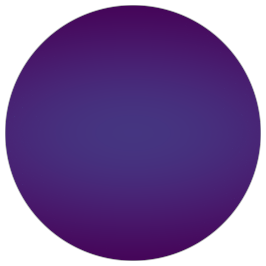
$\alpha_{x}=0.8$, $\alpha_{y}=0.2$, $\kappa=3.0$				$\alpha_{x}=0.8$, $\alpha_{y}=0.2$, $\kappa=4.0$

Figure 2. Convolving an SGGX with an SG kernel. Our fits closely matches the references in different configurations. Note that $\kappa$ is small because we only use SG to represent the clamped dot product term.

In §LABEL:sec:factorize_diffuse, we convolve an SGGX with a Spherical Gaussian (SG): $g(\omega)=\mathrm{SG}(\omega;n,\kappa)$ and compute a 3D mapping $\bm{\alpha}_{+}=M_{1}(\bm{\alpha},\kappa)$ (two channels). As we only consider a small range of $\kappa$, we use $20\times 20\times 20\times 2$ for its resolution in practice. In Fig 2, we visualize our fit using a single SGGX and compare it to the ground-truth convolution in different configurations. In Fig 1, we plot the RMSE error between our fit and the ground truth with varying $\kappa$.

Original	Kernel	Conv. Ours	Conv. Ref.	Original	Kernel	Conv. Ours	Conv. Ref.
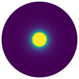
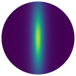
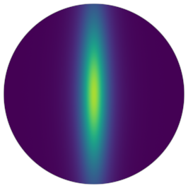
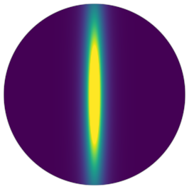
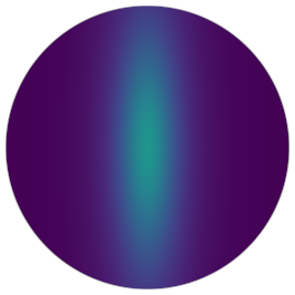
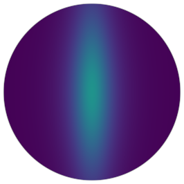
$\alpha_{x}=0.1$, $\alpha_{y}=0.7$, $\alpha=0.1$				$\alpha_{x}=0.1$, $\alpha_{y}=0.7$, $\alpha=0.2$
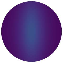
$\alpha_{x}=0.1$, $\alpha_{y}=0.7$, $\alpha=0.4$				$\alpha_{x}=0.1$, $\alpha_{y}=0.7$, $\alpha=0.6$
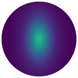
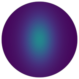
$\alpha_{x}=0.3$, $\alpha_{y}=0.5$, $\alpha=0.1$				$\alpha_{x}=0.3$, $\alpha_{y}=0.5$, $\alpha=0.2$
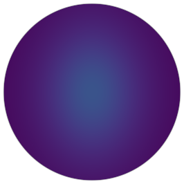
$\alpha_{x}=0.3$, $\alpha_{y}=0.5$, $\alpha=0.4$				$\alpha_{x}=0.3$, $\alpha_{y}=0.5$, $\alpha=0.6$
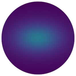
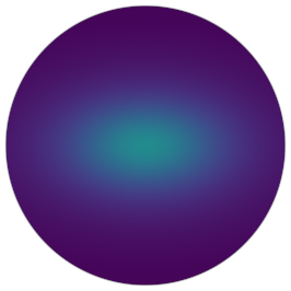
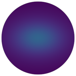
$\alpha_{x}=0.6$, $\alpha_{y}=0.4$, $\alpha=0.1$				$\alpha_{x}=0.6$, $\alpha_{y}=0.4$, $\alpha=0.2$
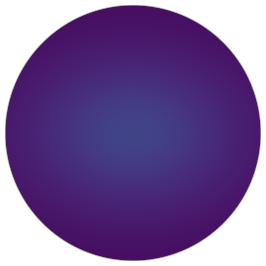
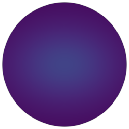
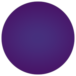
$\alpha_{x}=0.6$, $\alpha_{y}=0.4$, $\alpha=0.4$				$\alpha_{x}=0.6$, $\alpha_{y}=0.4$, $\alpha=0.6$
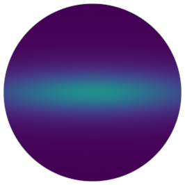
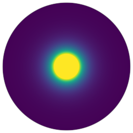
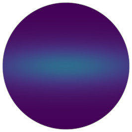
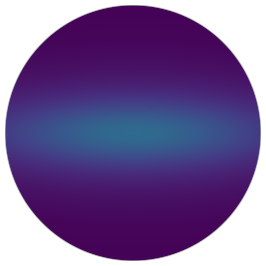
$\alpha_{x}=0.8$, $\alpha_{y}=0.2$, $\alpha=0.1$				$\alpha_{x}=0.8$, $\alpha_{y}=0.2$, $\alpha=0.2$
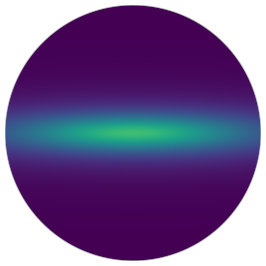
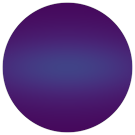
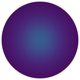
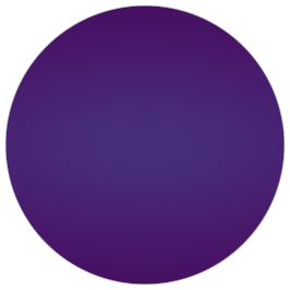
$\alpha_{x}=0.8$, $\alpha_{y}=0.2$, $\alpha=0.4$				$\alpha_{x}=0.8$, $\alpha_{y}=0.2$, $\alpha=0.6$

Figure 3. Convolving an SGGX with a GGX kernel. Our fits closely matches the references in different configurations.

In §LABEL:subsec:conv_with_ndf, we convolve an SGGX with a GGX microfacet distribution: $g(\omega_{h})=D(\omega_{h};n,\alpha)$ and compute a 3D mapping $\bm{\alpha}_{+}=M_{2}(\bm{\alpha},\alpha)$ (two channels). We use $50\times 50\times 50\times 2$ for its resolution in practice. Similarly, we provide visualization and error plots to compare our fit to the ground truth in Fig 1 and Fig 3.

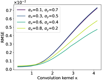
(a)

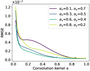
(b)

Figure 1. (a) RMSE of our SGGX-SG convolution fit with varying $\kappa$. Note that we only consider a small range of $\kappa$ because we only use SG to represent the clamped dot product term. (b) RMSE of our SGGX-GGX convolution fit with varying $\alpha$.

1.2. Aggregated Microfacet Distribution

In §LABEL:subsec:conv_with_ndf, we use a beta distribution to represent the roughness distribution $p_{\mathcal{A}}(\alpha)=\mathcal{B}(\alpha;a,b)$. Let $\mu$ and $\sigma^{2}$ be the mean and the variance, the shape parameters of a beta distribution can be estimated as

(2) $$\begin{split}a&=-\mu(\sigma^{2}+\mu^{2}-\mu)/\sigma^{2},\\ b&=(\sigma^{2}+\mu^{2}-\mu)(\mu-1)/\sigma^{2}.\\ \end{split}$$

	Map 1	Map 2	Map 3	Map 4	Map 5
$p(\alpha)$
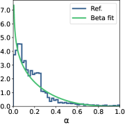
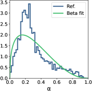
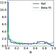
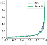
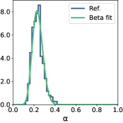
$D(\omega_{m})$

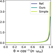
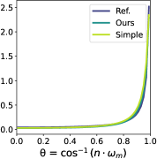
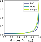
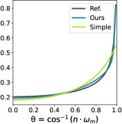
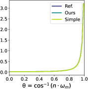
Figure 4. Fitting the distributions of a set of roughness maps as beta distributions and the aggregated microfacet distributions by our 2-lobe weighted sum.

We validate the effectiveness of this approach by estimating $p_{\mathcal{A}}(\alpha)$ from a set of roughness maps used for actual assets for the main article. Fig 4 shows the roughness maps, the ground-truth histograms and our estimated beta distributions. Our fits are reasonably accurate and adapt to the different modes of real data. It is clear that a Gaussian distribution would have exceeded the valid $[0,1]$ range of $\alpha$ (e.g. map 1, 3, and 4). A truncated Gaussian can be restricted within the valid range and may produce similar quality, but the fitting process is more tedious. We then validate the effectiveness of Eq. LABEL:eq:rough_var_two_lobe_fit by comparing our 2-lobe fit to the ground-truth aggregated microfacet distributions as well as a single-lobe fit with simple averaged roughness. Our fits are overall more accurate and guaranteed to be never worse than the simple fits.

1.3. Correction for Conditioned Angular Domain

We validate the approximation made in Eq. LABEL:eq:angular_domain in a set of configurations including different shapes of the SGGX and the angular domain $\mathcal{X}$. Fig 5 to 8 visualizes our approximation and compare it to the ground-truth. Our approximation qualitatively matches the geometric characteristics of the original distribution and the conditioned domain, and in general achieves reasonable accuracy. The source of error comes from the constant contribution assumption in the shape term in Eq. LABEL:eq:angular_domain. This results in under- or overestimates in some cases. For example, our approximation produces slightly darker results in Fig 6, row 2 and 3, but slightly brighter results in row 4. In Fig 8, row 5 and 6, our lobe shapes are slightly stretched compared to references.

2. Truncated Ellipsoid Primitive Projected Area

We provide an efficient Monte Carlo estimator to calculate the projected area of the intersection of a cube and an ellipsoid. We first uniformly sample points on the visible ellipsoid [Heitz et al., 2015]. Then, we cast a line from each point along $\omega$ to test if it intersects the cube. The ratio of intersection times the full ellipsoid projected area provides an estimator to $|B|_{\omega}$. Algorithm 1 provides the pseudocode. In practice, we optimize the implementation by using a fixed sample budget of $N=16$ and by early-exiting if the ellipsoid is fully contained by the cube or vice versa.

Algorithm 1 Computing the projected area along $\omega$ of a truncated ellipsoid primitive $B$.

1:function ProjectedArea($B$, $\omega$)

2:     $M\leftarrow$ the ellipsoid matrix, $c\leftarrow$ the ellipsoid center

3:     $Q\leftarrow$ the cube

4:     Compute an orthonormal basis $\Omega=(\omega_{x},\omega_{y},\omega)$ from $\omega$

5:     $M_{\omega}^{-1}\leftarrow\Omega^{T}M^{-1}\Omega$

6:     $M_{\omega xy}^{-1}$ $\leftarrow$ the upper left 2x2 block of $M_{\omega}^{-1}$

7:     Compute the Cholesky decomposition of $M_{\omega}^{-1}$: $M_{\omega}^{-1}=LL^{T}$

8:     for $i=1$ to $N$ do

9:         Sample a point on unit disk $(x,y)$ and lift it to the unit upper hemisphere: $p\leftarrow(x,y,\sqrt{1-x^{2}-y^{2}})$

10:         Warp $p$ to the visible ellipsoid surface: $p\leftarrow Lp$

11:         Transform $p$ back to world space: $p\leftarrow\Omega p+c$

12:         Cast a line $l$ that passes $p$ in direction $\omega$

13:         if $l$ intersects $Q$ then

14:              $m\leftarrow m+1$

15:         end if

16:     end for

17:     return $\frac{m}{N}\cdot\pi\sqrt{\det(M_{\omega xy}^{-1})}$

18:end function

3. Visibility Compression Details

As described in §LABEL:subsec:compression, we employ Clustered Principal Component Analysis (CPCA) to compress the aggregated visibility (both AIV and ABV). The method is similar to that of Sloan et al. [2003] and Liu et al. [2004], but we describe some of its details for completeness. Given a set of input visibility data, we first partition the angular domain: This is both to reduce the problem size and improve angular locality. Since we parameterize by the equal-area mapping [Clarberg, 2008], we simply partition the entire domain into $4\times 4$ angular tiles. CPCA is applied individually to each group of tiles that cover the same subset of the domain. Note that many tiles are completely visible or occluded and can be culled away early.

Let $C$ be the visibility matrix of a cluster of tiles where each column is one tile flattened to 1D and subtracted by the cluster mean. The standard principal component analysis (PCA) involves computing the (reduced) singular value decomposition (SVD) of $C$:

(3) $$C=U\Sigma V^{\mkern-1.5mu\mathsf{T}}.$$

Next, we take the top $k$ left-singular vectors from the $k$ leftmost columns of $U$ as the representative tiles (instead of the more common right-singular vectors from columns of $V$). For efficiency, we follow Sloan et al. [2003] and compute the eigendecomposition of either $CC^{\mkern-1.5mu\mathsf{T}}$ or $C^{\mkern-1.5mu\mathsf{T}}C$, whichever is smaller. Both produce eigenvalues equal to $\Sigma^{2}$. The eigenvectors of $CC^{\mkern-1.5mu\mathsf{T}}$ is $U$; The eigenvectors of $C^{\mkern-1.5mu\mathsf{T}}C$ is the right-singular vectors $V$ from which $U$ can be computed via $U=CV\Sigma^{-1}$. When possible, we only solve for the top eigenpairs by the Lanczos algorithm [Golub and Van Loan, 2013; Qiu, 2016].

Finally, each representative tile goes through wavelet compression with non-standard 2D Haar wavelet. During rendering, it is unnecessary to decompress the entire tile. The wavelet coefficients can be arranged as an implicit sparse quadtree that supports random access [Lalonde, 1997]. To evaluate visibility of a given direction, we can traverse a path down the tree, following a child if its basis supports the direction being evaluated.

Kernel	Clamped Orig.		Ref.		Ours

Figure 5. Convolving an SGGX with a GGX over an restricted domain $\mathcal{X}$. The kernel has roughness $\alpha=0.2$ and the original SGGX has roughness $\alpha_{x}=0.3,\alpha_{y}=0.3$. The contribution of the original distribution is clamped to black by $\mathcal{X}$.

Kernel	Clamped Orig.		Ref.		Ours

Figure 6. Convolving an SGGX with a GGX over an restricted domain $\mathcal{X}$. The kernel has roughness $\alpha=0.4$ and the original SGGX has roughness $\alpha_{x}=0.3,\alpha_{y}=0.3$. The contribution of the original distribution is clamped to black by $\mathcal{X}$.

Kernel	Clamped Orig.		Ref.		Ours

Figure 7. Convolving an SGGX with a GGX over an restricted domain $\mathcal{X}$. The kernel has roughness $\alpha=0.2$ and the original SGGX has roughness $\alpha_{x}=0.8,\alpha_{y}=0.2$. The contribution of the original distribution is clamped to black by $\mathcal{X}$.

Kernel	Clamped Orig.		Ref.		Ours

Figure 8. Convolving an SGGX with a GGX over an restricted domain $\mathcal{X}$. The kernel has roughness $\alpha=0.4$ and the original SGGX has roughness $\alpha_{x}=0.8,\alpha_{y}=0.2$. The contribution of the original distribution is clamped to black by $\mathcal{X}$.

References

- [1]
- Clarberg [2008] Petrik Clarberg. 2008. Fast Equal-Area Mapping of the (Hemi)Sphere using SIMD. J. Graph. Tools 13, 3 (2008), 53–68. https://doi.org/10.1080/2151237X.2008.10129263
- Golub and Van Loan [2013] Gene H Golub and Charles F Van Loan. 2013. Matrix computations. JHU press.
- Heitz et al. [2015] Eric Heitz, Jonathan Dupuy, Cyril Crassin, and Carsten Dachsbacher. 2015. The SGGX microflake distribution. ACM Trans. Graph. 34, 4 (2015), 48:1–48:11. https://doi.org/10.1145/2766988
- Lalonde [1997] Paul Lalonde. 1997. Representations and uses of light distribution functions. Ph. D. Dissertation. University of British Columbia.
- Liu et al. [2004] Xinguo Liu, Peter-Pike J. Sloan, Heung-Yeung Shum, and John Snyder. 2004. All-Frequency Precomputed Radiance Transfer for Glossy Objects. In Proceedings of the 15th Eurographics Workshop on Rendering Techniques, Norköping, Sweden, June 21-23, 2004, Alexander Keller and Henrik Wann Jensen (Eds.). Eurographics Association, 337–344. https://doi.org/10.2312/EGWR/EGSR04/337-344
- Qiu [2016] Yixuan Qiu. 2016. Spectra: C++ library for large scale eigenvalue problems. https://spectralib.org/ (Date accessed: 07.08.2024).
- Sloan et al. [2003] Peter-Pike Sloan, Jesse Hall, John Hart, and John Snyder. 2003. Clustered Principal Components for Precomputed Radiance Transfer. ACM Trans. Graph. 22, 3 (jul 2003), 382–391. https://doi.org/10.1145/882262.882281