Randomized Lower Bounds for Tarski Fixed Points in High Dimensions

Abstract

The Knaster-Tarski theorem, also known as Tarski’s theorem, guarantees that every monotone function defined on a complete lattice has a fixed point. We analyze the query complexity of finding such a fixed point on the $k$-dimensional grid of side length $n$ under the $\leq$ relation. Specifically, there is an unknown monotone function $f:\{0,1,\ldots,n-1\}^{k}\to\{0,1,\ldots,n-1\}^{k}$ and an algorithm must query a vertex $v$ to learn $f(v)$.

Our main result is a randomized lower bound of $\Omega\left(k+\frac{k\cdot\log{n}}{\log{k}}\right)$ for the $k$-dimensional grid of side length $n$, which is nearly optimal in high dimensions when $k$ is large relative to $n$. As a corollary, we characterize the randomized and deterministic query complexity of the Tarski search problem on the Boolean hypercube $\{0,1\}^{k}$ as $\Theta(k)$.

1 Introduction

The Knaster-Tarski theorem, also known as Tarski’s theorem, guarantees that every monotone function $f:\mathcal{L}\to\mathcal{L}$ defined over a complete lattice $(\mathcal{L},\leq)$ has a fixed point. Tarski proved the most general form of the theorem [Tar55]:

Let $(\mathcal{L},\leq)$ be a complete lattice and let $f:\mathcal{L}\to\mathcal{L}$ be an order-preserving (monotone) function with respect to $\leq$. Then the set of fixed points of $f$ in $\mathcal{L}$ forms a complete lattice under $\leq$.

An earlier version was shown by Knaster and Tarski [KT28], who established the result for the special case where $\mathcal{L}$ is the lattice of subsets of a set (i.e. the power set lattice).

This is a classical theorem with broad applications. For example, in formal semantics of programming languages and abstract interpretation, the existence of fixed points can be exploited to guarantee well-defined semantics for a recursive algorithm [For05]. In game theory, Tarski’s theorem implies the existence of pure Nash equilibria in supermodular games [EPRY19]. Surprisingly, it is not fully understood how efficiently Tarski fixed points can be found.

Formally, for $k,n\in\mathbb{N}$, let $\mathcal{L}_{n}^{k}=\{0,1,\ldots,n-1\}^{k}$ be the $k$-dimensional grid of side length $n$. Let $\leq$ be the binary relation where for vertices ${a}=(a_{1},\ldots,a_{k})\in\mathcal{L}_{n}^{k}$ and ${b}=(b_{1},\ldots,b_{k})\in\mathcal{L}_{n}^{k}$, we have ${a}\leq{b}$ if and only if $a_{i}\leq b_{i}$ for each $i\in[k]$. We consider the lattice $(\mathcal{L}_{n}^{k},\leq)$. A function $f:\mathcal{L}_{n}^{k}\to\mathcal{L}_{n}^{k}$ is monotone if ${a}\leq{b}$ implies that $f({a})\leq f({b})$. Tarski’s theorem states that the set $P$ of fixed points of $f$ is non-empty and that the system $(P,\leq)$ is itself a complete lattice [Tar55].

In this paper, we focus on the query model, where there is an unknown monotone function $f:\mathcal{L}_{n}^{k}\to\mathcal{L}_{n}^{k}$. An algorithm has to probe a vertex $v$ in order to learn the value of the function $f(v)$. The task is to find a fixed point of $f$ by probing as few vertices as possible. The randomized query complexity is the expected number of queries required to find a solution with a probability of at least $9/10$ by the best algorithm , where the expectation is taken over the coin tosses of the algorithm.

There are two main algorithmic approaches for finding a Tarski fixed point. The first approach is a divide-and-conquer method that yields an upper bound of $O\left((\log{n})^{\lceil\frac{k+1}{2}\rceil}\right)$ for any fixed $k$ due to [CL22], which improves an algorithm of [FPS22].

The second is a path-following method that initially queries the vertex $\mathbf{0}=(0,\ldots,0)$ and proceeds by following the directional output of the function. With each function application, at least one coordinate is incremented, which guarantees that a fixed point is reached within $O(nk)$ queries.

[EPRY19] proved a randomized query complexity lower bound of $\Omega\left(\log^{2}(n)\right)$ on the 2D grid of side length $n$, which implies the same lower bound for the $k$-dimensional grid of side length $n$ when $k$ is constant. This lower bound shows that the divide-and-conquer algorithm is optimal for dimensions $k=2$ and $k=3$.

For dimension $k\geq 4$, there is a growing gap between the best-known upper and lower bounds, since the upper bound given by the divide-and-conquer algorithm has an exponential dependence on $k$. Meanwhile, the path-following method provides superior performance in high dimensions, such as the Boolean hypercube $\{0,1\}^{k}$, where it achieves an upper bound of $O(k)$.

1.1 Our Contributions

Let ${TARSKI}(n,k)$ denote the Tarski search problem on the $k$-dimensional grid of side length $n$.

Definition 1 (${TARSKI}(n,k)$).

Let $k,n\in\mathbb{N}$. Given oracle access to an unknown monotone function $f:\mathcal{L}_{n}^{k}\to\mathcal{L}_{n}^{k}$, find a vertex $x\in\mathcal{L}_{n}^{k}$ with $f(x)=x$ using as few queries as possible.

Our main result is the following:

Theorem 1.

There is a constant $c>0$ such that for all $k,n\in\mathbb{N}$, the randomized query complexity of ${TARSKI}(n,k)$ is at least $c\cdot\left(k+\frac{k\cdot\log{n}}{\log{k}}\right)$.

The lower bound in Theorem 1 is sharp for constant $n\geq 2$ and nearly optimal in the general case when $k$ is large relative to $n$.

Theorem 1 gives a characterization of $\Theta(k)$ for the randomized and deterministic query complexity on the Boolean hypercube $\{0,1\}^{k}$, since the deterministic path-following method that iteratively applies the function starting from vertex $\mathbf{0}=(0,\ldots,0)$ finds a solution within $O(k)$ queries. No lower bound better than $\Omega(1)$ was known for the Boolean hypercube.

Corollary 1.

The randomized and deterministic query complexity of ${TARSKI}(2,k)$ is $\Theta(k)$.

We obtain Theorem 1 by designing the following family of monotone functions.

Definition 2 (Set of functions $\mathcal{F}$).

For each $a\in\mathcal{L}_{n}^{k}$, we define a function $f^{a}:\mathcal{L}_{n}^{k}\to\mathcal{L}_{n}^{k}$ coordinate by coordinate. That is, for each $v=(v_{1},\ldots,v_{k})\in\mathcal{L}_{n}^{k}$ and $i\in[k]$, let

$$f^{a}_{i}(v)=\begin{cases}v_{i}-1&\text{ if $(v_{i}>a_{i})$ and $(v_{j}\leq a_{j}$ for all $j<i)$}\\ v_{i}+1&\text{ if $(v_{i}<a_{i})$ and $(v_{j}\geq a_{j}$ for all $j<i)$}\\ v_{i}&\text{ otherwise.}\end{cases}$$ (1)

Let $f^{a}(v)=(f^{a}_{1}(v),\ldots,f^{a}_{k}(v))$. Define $\mathcal{F}=\{f^{a}\mid a\in\mathcal{L}_{n}^{k}\}$.

The intuition is that the first digit that is too low and the first digit that is too high both get pushed towards their correct value. An example of a function from Definition 2 is shown in Figure 1.

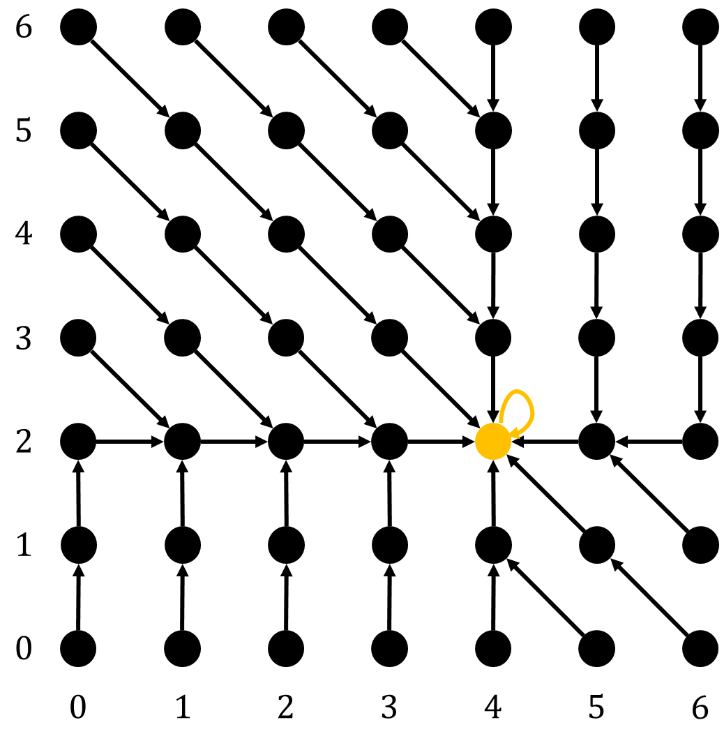
Figure 1: Example of a function $f^{a}$ from Definition 2 where $a=(2,4)$ and the grid dimensions are $n=7$ and $k=2$. The function $f^{a}$ has a unique fixed point at $a=(2,4)$.

For $k=2$, this construction is similar to the herringbone construction of [EPRY19]; however, our construction does not induce a lower bound of $\log^{2}(n)$ on the 2D grid since the shape of the path from $(0,0)$ or $(n-1,n-1)$ to the fixed point is too predictable.

The real strength of our construction emerges for large $k$, where the herringbone is not defined. Critically, a function $f\in\mathcal{F}$ has the property that $f(v)$ differs from $v$ in at most $2$ dimensions for all $v$, no matter how large $k$ is. This makes it difficult to derive information about more than a constant number of dimensions with a single query. The proof of Theorem 1 makes this intuition precise.

1.2 Related Work

Tarski fixed points.

Algorithms for the problem of finding Tarski fixed points on the $k$-dimensional grid of side length $n$ have only recently been considered. [DQY20] gave an $O(\log^{k}(n))$ divide-and-conquer algorithm. [FPS22] gave an $O(\log^{2}(n))$ algorithm for the 3D grid and used it to construct an $O(\log^{2\lceil k/3\rceil}(n))$ algorithm for the $k$-dimensional grid of side length $n$. [CL22] extended their ideas to get an $O(\log^{\lceil(k+1)/2\rceil}(n))$ algorithm.

[EPRY19] showed a lower bound of $\Omega(\log^{2}(n))$ for the 2D grid, implying the same lower bound for the $k$-dimensional grid of side length $n$. This bound is tight for $k=2$ and $k=3$, but there is an exponential gap for larger $k$. They also showed that the problem is in both PLS and PPAD, which by the results of [FGHS22] implies it is in CLS.

[CLY23] give a black-box reduction from the Tarski problem to the same problem with an additional promise that the input function has a unique fixed point. This result implies that the Tarski problem and the unique Tarski problem have the same query complexity.

Next we briefly summarize query and communication complexity results for two problems representative for the classes PLS and PPAD, respectively. These problems are finding a local minimum and a Brouwer fixed point, respectively. In both cases, the existing lower bounds also rely on hidden path constructions.

Brouwer fixed points.

In the Brouwer search problem, we are given a function $f:[0,1]^{d}\to[0,1]^{d}$ that is $L$-Lipschitz, for some constant $L>1$. The task is to find a fixed point of $f$ using as few queries to $f$ as possible. The existence of a fixed point is guaranteed by Brouwer’s fixed point theorem. The query complexity of computing an $\varepsilon$-approximate Brouwer fixed point was studied in a series of papers starting with [HPV89], which introduced a construction where the function is induced by a hidden walk. This was later improved by [CD05] and [CT07].

Local minima.

In the local search problem, we are given a graph $G=(V,E)$ and a function $f:V\to\mathbb{R}$. A vertex $v$ is a local minimum if $f(v)\leq f(u)$ for all $(u,v)\in E$. An algorithm can probe a vertex $v$ to learn its value $f(v)$. The task is to find a vertex that is a local minimum using as few queries as possible. [Ald83] obtains a lower bound of $\Omega(2^{k/2-o(k)})$ on the query complexity for the Boolean hypercube $\{0,1\}^{k}$ by a random walk analysis. Aldous’ lower bound for the hypercube was later improved by [Aar06] to $\Omega(2^{k/2}/k^{2})$ via a relational adversary method inspired from quantum computing. [Zha09] further improved this lower bound to $\Theta(2^{k/2}\cdot\sqrt{k})$ via a “clock”-based random walk construction. Meanwhile, [LTT89] developed a deterministic divide-and-conquer algorithm.

For the $k$-dimensional grid $[n]^{k}$, [Aar06] used the relational adversary method to show a randomized lower bound of $\Omega(n^{k/2-1}/\log n)$ for every constant $k\geq 3$. [Zha09] proved a randomized lower bound of $\Omega(n^{k/2})$ for every constant $k\geq 4$. The work of [SY09] closed further gaps in the quantum setting as well as the randomized $k=2$ case.

For general graphs, [SS04] gave a quantum lower bound of $\Omega\left(\sqrt[8]{\frac{s}{\Delta}}/\log(n)\right)$, where $n$ is the number of vertices of the graph, $s$ is the separation number, and $\Delta$ the maximum degree. [BCR24] improved this lower bound to $\Omega\left(\sqrt[4]{\frac{s}{\Delta}}\right)$ for randomized algorithms and also obtained a randomized lower bound of $\Omega\left(\frac{n^{1.5}}{g}\right)$, where $g$ is the vertex congestion of the graph. [SS04] also gave an upper bound of $O((s+\Delta)\cdot\log n)$, which was obtained by refining a divide-and-conquer algorithm of [LTT89].

[DR10] gave lower bounds for Cayley graphs as a function of the number of vertices and the diameter of the graph. [Ver06] obtained upper bounds as a function of the genus of the graph.

[BDN19] studied the communication complexity of local search; this captures distributed settings, where data is stored on different computers.

2 Properties of the family of functions $\mathcal{F}$

In this section we show that each function in the family $\mathcal{F}$ of Definition 2 is monotone and has a unique fixed point.

Lemma 1.

For each $a\in\mathcal{L}_{n}^{k}$, the function $f^{a}$ from Definition 2 is monotone.

Proof.

Consider two arbitrary vertices $u,v\in\mathcal{L}_{n}^{k}$ with $u\leq v$. Suppose towards a contradiction that $f^{a}(u)\leq f^{a}(v)$ does not hold. Then there exists an index $i\in[k]$ such that $f^{a}_{i}(u)>f^{a}_{i}(v)$. Since $u\leq v$, we have $u_{i}\leq v_{i}$, so at least one of $f^{a}_{i}(u)>u_{i}$ or $f^{a}_{i}(v)<v_{i}$ holds.

Case 1: $f^{a}_{i}(u)>u_{i}$.

By definition of $f^{a}$, we then have $u_{i}<a_{i}$ and $u_{j}\geq a_{j}$ for all $j<i$. Since $u\leq v$, we also have $v_{j}\geq a_{j}$ for all $j<i$. Furthermore, we have $v_{i}=u_{i}$, or $v_{i}=u_{i}+1$, or $v_{i}\geq u_{i}+2$. We consider a few sub-cases:

1. ($v_{i}=u_{i}$). Then $f^{a}_{i}(v)=v_{i}+1=u_{i}+1=f^{a}_{i}(u)$.

2. ($v_{i}=u_{i}+1$). Then $v_{i}\leq a_{i}$, so $f^{a}_{i}(v)\geq v_{i}=u_{i}+1=f^{a}_{i}(u)$.

3. ($v_{i}\geq u_{i}+2$). Then $f^{a}_{i}(v)\geq v_{i}-1\geq u_{i}+1=f^{a}_{i}(u)$.

In each subcase (a-c), we have $f^{a}_{i}(v)\geq f^{a}_{i}(u)$. This is in contradiction with $f^{a}_{i}(u)>f^{a}_{i}(v)$, thus case 1 cannot occur.

Case 2: $f^{a}_{i}(v)<v_{i}$.

By definition of $f^{a}$, we then have $v_{i}>a_{i}$ and $v_{j}\leq a_{j}$ for all $j<i$. Since $u\leq v$, we also have $u_{j}\leq a_{j}$ for all $j<i$. Furthermore, we have $u_{i}=v_{i}$, or $u_{i}=v_{i}-1$, or $u_{i}\leq v_{i}-2$. We consider a few sub-cases:

1. ($u_{i}=v_{i}$). Then $f^{a}_{i}(u)=u_{i}-1=v_{i}-1=f^{a}_{i}(v)$.

2. ($u_{i}=v_{i}-1$). Then $u_{i}\geq a_{i}$, so $f^{a}_{i}(u)\leq u_{i}=v_{i}-1=f^{a}_{i}(v)$.

3. ($u_{i}\leq v_{i}-2$). Then $f^{a}_{i}(u)\leq u_{i}+1\leq v_{i}-1=f^{a}_{i}(v)$.

In each subcase (a-c), we have $f^{a}_{i}(u)\leq f^{a}_{i}(v)$. This in contradiction with $f^{a}_{i}(u)>f^{a}_{i}(v)$, thus case $2$ cannot occur either.

In both cases $1$ and $2$ we reached a contradiction, so the assumption that $f^{a}(u)\leq f^{a}(v)$ does not hold must have been false. Thus $f^{a}$ is monotone. ∎

Lemma 2.

For each $a\in\mathcal{L}_{n}^{k}$, the function $f^{a}\in\mathcal{F}$ has a unique fixed point at $a$.

Proof.

By definition of $f^{a}$ we have $f^{a}(a)=a$, so $a$ is a fixed point of $f^{a}$.

Let $v\neq a$. Then there exists $i\in[k]$ such that $v_{i}\neq a_{i}$. Let $i$ be the minimum such index. We have two cases:

• ($v_{i}<a_{i}$): Then $f^{a}_{i}(v)=v_{i}+1$, so $f^{a}(v)\neq v$.

• ($v_{i}>a_{i}$): Then $f^{a}_{i}(v)=v_{i}-1$, so $f^{a}(v)\neq v$.

In both cases $v$ is not a fixed point, so $a$ is the only fixed point of $f^{a}$. ∎

3 Lower bounds

3.1 Lower bound for the Boolean hypercube

Using the family of functions $\mathcal{F}$ from Definition 2, we can now prove a randomized lower bound of $\Omega(k)$ for the Boolean hypercube $\{0,1\}^{k}$.

Proposition 1.

The randomized query complexity of $TARSKI(2,k)$ is $\Omega(k)$.

Proof.

We proceed by invoking Yao’s lemma. Let $\mathcal{U}$ be the uniform distribution over the set of functions $\mathcal{F}$. Let $\mathcal{A}$ be the deterministic algorithm with the smallest possible expected number of queries that succeeds with probability at least $4/5$, where both the expected query count and the success probability are for input drawn from $\mathcal{U}$. The algorithm $\mathcal{A}$ exists since there is a finite number of deterministic algorithms for this problem, so the minimum is well defined.

Let $D$ be the expected number of queries issued by $\mathcal{A}$ on input drawn from $\mathcal{U}$. Let $R$ be the randomized query complexity of $TARSKI(2,k)$; i.e. the expected number of queries required to succeed with probability at least $9/10$. Then Yao’s lemma ([Yao77], Theorem 3) yields $2R\geq D$. Therefore it suffices to lower bound $D$.

For each $t\in\mathbb{N}$, let

• $\mathcal{H}_{t}$ denote the history of queries and responses received at steps $1,\ldots,t$.

• $\mathcal{I}_{t}=\Bigl{\{}i\in[k]\mid\mathcal{A}\;\mbox{ knows }a_{i}\mbox{ with certainty given the history }\mathcal{H}_{t}\Bigr{\}}$.

• $v^{t}$ denote the $t$-th query submitted by $\mathcal{A}$.

We prove by induction on $t$ that $\mathcal{I}_{t}$ is all the information that the algorithm $\mathcal{A}$ has by the end of round $t$. Clearly $\mathcal{I}_{0}=\emptyset$ since the algorithm has not made any queries so any input function is equally likely. We assume the inductive hypothesis holds for $t-1$ and prove it for $t$. We consider the indices where $v^{t}$ has zeroes and divide in two cases; the analysis for indices where $v^{t}$ has ones is symmetric. Initialize $\mathcal{I}_{t}=\mathcal{I}_{t-1}$. We explain in each case what new indices may enter $\mathcal{I}_{t}$.

1. There exists $i\in[k]$ such that $\bigl{(}v^{t}_{i}=0$ and $f^{a}_{i}(v^{t})=1\bigr{)}$. This implies three things:

   • $a_{i}=1$, so $i$ is added to $\mathcal{I}_{t}$.

   • For all $j<i$ such that $v^{t}_{j}=0$, it must be the case that $a_{j}=0$; otherwise, the bit at index $j$ would have been corrected to a $1$ instead of the bit at index $i$ getting corrected. Therefore, each such $j$ is added to $\mathcal{I}_{t}$.

   • The algorithm does not learn anything about the bits at locations $j>i$ with $v^{t}_{j}=0$, since regardless of the value of $a_{j}$, we have $f^{a}_{j}(v^{t})=0$. No such $j$ is added to $\mathcal{I}_{t}$, though some may have already been in $\mathcal{I}_{t-1}$.

2. There is no $i\in[k]$ such that $\bigl{(}v^{t}_{i}=0$ and $f^{a}_{i}(v^{t})=1\bigr{)}$. Then for all $j\in[k]$ such that $v_{j}^{t}=0$, it must have been the case that $a_{j}=0$. Therefore, all such $j$ are added to $\mathcal{I}_{t}$.

In either case (i) or (ii), the value of $f^{a}_{i}(v^{t})$ for indices $i\in[k]$ with $v^{t}_{i}=0$ gives $\mathcal{A}$ no information about indices $j\in[k]$ with $v^{t}_{j}=1$, as the value of $f^{a}(v^{t})$ at such $j$ depends only on other indices $\ell\in[k]$ where $v^{t}_{\ell}=1$.

Thus for each index $j\in[k]$, either $j\in\mathcal{I}_{t}$ (and so the algorithm $\mathcal{A}$ knows the bit $a_{j}$ with certainty) or the posterior for $a_{j}$ remains the uniform distribution. This completes the inductive step.

Next we argue that the expected number of bits learned with each query is upper bounded by a constant, that is $\operatorname{\mathbb{E}}[|\mathcal{I}_{t}|-|\mathcal{I}_{t-1}|\mid\mathcal{H}_{t-1}]\leq 4$.

$a$	$0$	$0$	$1$	$1$	$1$	$1$	$0$
$v^{1}$	$0$	$1$	$1$	$1$	$0$	$0$	$1$
$f^{a}(v^{1})$	$0$	$0$; $c_{1}(1)$	$1$	$1$	$1$; $c_{1}(0)$	$0$	$1$
$v^{2}$	$0$	$0$	$1$	$0$	$1$	$0$	$1$
$f^{a}(v^{2})$	$0$	$0$	$1$	$0$; $c_{2}(0)$	$1$	$0$	$0$; $c_{2}(1)$
$v^{3}$	$0$	$0$	$1$	$1$	$1$	$0$	$0$
$f^{a}(v^{3})$	$0$	$0$	$1$	$1$	$1$	$1$; $c_{3}(0)$	$0$

Figure 2: An example series of three queries for $n=8$. The red cells indicate the corresponding $\Delta_{t}(0)$, the blue cells indicate the set $\Delta_{t}(1)$, and the gray cells indicate the set $\mathcal{I}_{t}$. The finite values of $c_{t}(b)$ are labelled. For the third query, $c_{3}(1)=\infty$.

For $b\in\{0,1\}$, let $c_{t}(b)$ be the index of the bit where $v_{c_{t}(b)}^{t}=b$ and $f^{a}_{c_{t}(b)}(v^{t})=1-b$, or $c_{t}(b)=\infty$ if no such index exists. Then define $\Delta_{t}(b)$ as:

$$\Delta_{t}(b)=\left\{i\mid i\not\in\mathcal{I}_{t-1},v_{i}^{t}=b,\mbox{ and }i\leq c_{t}(b)\right\}\,.$$ (2)

In other words $\Delta_{t}(b)$ is precisely the set of indices $i\in[k]$ added to $\mathcal{I}_{t}$ (which were not in $\mathcal{I}_{t-1}$) with the property that $v_{i}^{t}=b$. We therefore have

$$\Delta_{t}(0)\cup\Delta_{t}(1)=\mathcal{I}_{t}\setminus\mathcal{I}_{t-1}\,.$$ (3)

The distribution of $|\Delta_{t}(b)|$ can be bounded effectively. For any $C\in\mathbb{N}$, we have $|\Delta_{t}(b)|>C$ only if the first $C$ indices $i\in[k]$ with the property that both $i\not\in\mathcal{I}_{t-1}$ and $v_{i}^{t}=b$ are guessed correctly, i.e. $a_{i}=b$. Therefore:

$$\Pr\bigl{[}|\Delta_{t}(b)|>C\mid\mathcal{H}_{t-1}\bigr{]}\leq 2^{-C}\,.$$ (4)

We can bound the expected value of $|\Delta_{t}(b)|$ as:

$$\mathbb{E}\bigl{[}|\Delta_{t}(b)|\mid\mathcal{H}_{t-1}\bigr{]} =\sum_{C=0}^{\infty}\Pr\bigl{[}|\Delta_{t}(b)|>C\mid\mathcal{H}_{t-1}\bigr{]}$$ (By Lemma 4)

$$\leq\sum_{C=0}^{\infty}2^{-C}$$ (By (4))

$$=2\,.$$ (5)

Using (3) and (5), we get:

$$\mathbb{E}\bigl{[}|\mathcal{I}_{t}|-|\mathcal{I}_{t-1}|\mid\mathcal{H}_{t-1}\bigr{]} =\mathbb{E}\bigl{[}|\Delta_{t}(0)|\mid\mathcal{H}_{t-1}\bigr{]}+\mathbb{E}\bigl{[}|\Delta_{t}(1)|\mid\mathcal{H}_{t-1}\bigr{]}\leq 2+2=4\,.$$ (6)

Since the upper bound of $4$ applies for all histories $\mathcal{H}_{t-1}$, taking expectation over all possible histories gives:

$$\mathbb{E}\bigl{[}|\mathcal{I}_{t}|-|\mathcal{I}_{t-1}|\bigr{]}\leq 4\qquad\forall t\in\mathbb{N}\,.$$ (7)

Since $|\mathcal{I}_{0}|=0$, inequality (7) implies $\mathbb{E}\bigl{[}|\mathcal{I}_{t}|\bigr{]}\leq 4t$. Thus $\mathbb{E}\bigl{[}|\mathcal{I}_{t}|\bigr{]}<5t$ for all $t\in\mathbb{N}^{*}$.

Let $T=k/100$. Then by Markov’s inequality applied to the random variable $\mathcal{I}_{T}$, we have

$$\Pr\bigl{[}|\mathcal{I}_{T}|\geq k\bigr{]}\leq\frac{\mathbb{E}\bigl{[}|\mathcal{I}_{T}|\bigr{]}}{k}<\frac{5T}{k}=1/20\,.$$ (8)

When $|\mathcal{I}_{T}|<k$, algorithm $\mathcal{A}$ makes an error with probability at least $1/2$ since it would have to guess at least one bit of $a$. Since $\mathcal{A}$ succeeds with probability at least $4/5$, we must have $|\mathcal{I}_{T}|=k$ with probability at least $3/5$.

Thus $\mathcal{A}$ issues more than $k/100$ queries with probability at least $1-1/20-2/5=11/20$. Therefore the expected number of queries issued by $\mathcal{A}$ is $D>(11/20)\cdot(k/100)\in\Omega(k)$. ∎

3.2 Lower bound for the $k$-dimensional grid of side length $n$

In this section we show the randomized lower bound of $\Omega(k)$ also holds for $TARSKI(n,k)$. Afterwards, we prove the construction from Definition 2 also yields a lower bound of $\Omega\left(\frac{k\log{n}}{\log(k)}\right)$ for the $k$-dimensional grid of side length $n$.

Lemma 3.

The randomized query complexity of $TARSKI(n,k)$ is at least the randomized query complexity of $TARSKI(2,k)$.

Proof.

We show a reduction from $TARSKI(2,k)$ to $TARSKI(n,k)$. Let $f^{*}:\{0,1\}^{k}\to\{0,1\}^{k}$ be an arbitrary instance of $TARSKI(2,k)$. As such, $f^{*}$ is monotone.

Let $g:\{0,1,\ldots,n-1\}^{k}\to\{0,1\}^{k}$ be the clamp function, given by

$$g(v)=(g_{1}(v),\ldots,g_{k}(v)),\mbox{ where }g_{i}(v)=\min(v_{i},1)\;\forall i\in[k]\,.$$ (9)

Then define $f:\{0,1,\ldots,n-1\}^{k}\to\{0,1,\ldots,n-1\}^{k}$ as $f(v)=f^{*}(g(v))$.

To show that $f$ is monotone, let $u,v\in\{0,1,\ldots,n-1\}^{k}$ be arbitrary vertices with $u\leq v$. Then $g(u)\leq g(v)$, so $f(u)=f^{*}(g(u))\leq f^{*}(g(v))=f(v)$ by monotonicity of $f^{*}$. Thus $f$ is monotone and has a fixed point.

Every vertex $u\in\{0,1,\ldots,n-1\}^{k}\setminus\{0,1\}^{k}$ is not a fixed point of $f$, since $f(u)\in\{0,1\}^{k}$. Every fixed point $u\in\{0,1\}^{k}$ of $f$ is also a fixed point of $f^{*}$ since $g(u)=u$ for all $u\in\{0,1\}^{k}$. Therefore all fixed points of $f$ are also fixed points of $f^{*}$.

A query to $f$ may be simulated using exactly one query to $f^{*}$ since computing $g$ does not require any knowledge of $f^{*}$.

Therefore any algorithm that finds a fixed point of $f$ can also be used to find a fixed point of $f^{*}$ in the same number of queries. Therefore the randomized query complexity of $TARSKI(n,k)$ is greater than or equal to the randomized query complexity of $TARSKI(2,k)$. ∎

Applying Lemma 3 to Proposition 1 directly gives the following corollary.

Corollary 2.

The randomized query complexity of $TARKSI(n,k)$ is $\Omega(k)$.

We also get the following lower bound.

Proposition 2.

The randomized query complexity of $TARSKI(n,k)$ is $\Omega\left(\frac{k\log(n)}{\log(k)}\right)$.

Proof.

We proceed by invoking Yao’s lemma. Let $\mathcal{U}$ be the uniform distribution over the set of functions $\mathcal{F}$. Let $\mathcal{A}$ be the deterministic algorithm with the smallest possible expected number of queries that succeeds with probability at least $4/5$, where both the expected query count and the success probability are for input drawn from $\mathcal{U}$. The algorithm $\mathcal{A}$ exists since there is a finite number of deterministic algorithms for this problem, so the minimum is well defined.

Let $D$ be the expected number of queries issued by $\mathcal{A}$ on input drawn from $\mathcal{U}$. Let $R$ be the randomized query complexity of $TARSKI(n,k)$; i.e. the expected number of queries required to succeed with probability at least $9/10$. Then Yao’s lemma ([Yao77], Theorem 3) yields $2R\geq D$. Therefore it suffices to lower bound $D$.

For each vertex $v\in\{0,\ldots,n-1\}^{k}$, let $Q_{v}$ be the set of possible outputs when plugging in $v$:

$$Q_{v}=\bigl{\{}f^{a}(v)\mid a\in\{0,1,\ldots,n-1\}^{k}\bigr{\}}\,.$$ (10)

We next bound $|Q_{v}|$. By the definition of $f^{a}$, the vertex $f^{a}(v)$ differs from $v$ in at most two coordinates: the first $i\in[k]$ such that $v_{i}>a_{i}$ (if any) and the first $j\in[k]$ such that $v_{j}<a_{j}$ (if any). Each of $i$ and $j$ have $k+1$ options, corresponding to the $k$ dimensions and the possibility that no such dimension exists. Therefore

$$|Q_{v}|\leq(k+1)^{2}\,.$$ (11)

Recall that $\mathcal{A}$ is defined to the best deterministic algorithm that succeeds on $\mathcal{U}$ with probability at least $4/5$. Since $\mathcal{U}$ is uniform over $\mathcal{F}$, there must exist at least $(4/5)\cdot n^{k}$ inputs on which $\mathcal{A}$ outputs a fixed point. Then the decision tree of $\mathcal{A}$ must have at least $(4/5)\cdot n^{k}$ leaves since all supported inputs have different and unique fixed points. Every node of this tree has at most $(k+1)^{2}$ children, since $|Q_{v}|\leq(k+1)^{2}$ for all $v$ by (11). Therefore the average depth of the leaves is at least

$$\log_{(k+1)^{2}}\Bigl{(}(4/5)n^{k}\Bigr{)}-1=\frac{\log_{2}((4/5)n^{k})}{\log_{2}((k+1)^{2})}-1\geq\frac{k\log_{2}(n)-1}{2\log_{2}(k)+2}-1\in\Omega\left(\frac{k\log n}{\log k}\right)\,.$$ (12)

Then on input distribution $\mathcal{U}$, algorithm $\mathcal{A}$ issues an expected number of queries of $D\in\Omega(\frac{k\log n}{\log k})$. Thus the randomized query complexity of $TARSKI(n,k)$ is $\Omega(\frac{k\log n}{\log k})$ as required. ∎

The proof of Theorem 1 follows from Corollary 2 and Proposition 2.

Proof of Theorem 1.

The randomized query complexity of $TARSKI(n,k)$ is $\Omega(k)$ by Corollary 2 and $\Omega\left(\frac{k\log{n}}{\log(k)}\right)$ by Proposition 2. This implies a lower bound of $\Omega\left(k+\frac{k\log{n}}{\log(k)}\right)$ as required. ∎

4 Upper bound for the family of functions $\mathcal{F}$

It may seem that the family of instances $\mathcal{F}$ from Definition 2 should in fact yield a lower bound of $\Omega\left(k\log{n}\right)$. Intuitively, $k\log{n}$ may be achievable since the only feedback an algorithm receives with each query on an input from $\mathcal{F}$ is whether the query is too high or too low on roughly two coordinates. However, this intuition turns out to be incorrect when $n$ is close to $k$. The next proposition shows that the family of functions $\mathcal{F}$ cannot yield a lower bound of $\Omega\left(k\log{n}\right)$ for all $k$ and $n$.

Proposition 3.

There is a deterministic $O(k+n)$-query algorithm for $TARSKI(n,k)$ on the set of functions $\mathcal{F}$.

Proof.

For each coordinate $i\in[k]$ and each query index $t$, let $x^{t}_{i}$ and $y^{t}_{i}$ be the minimum and maximum possible values of $a_{i}$ given the first $t$ queries the algorithm makes. For example, $x^{0}_{i}=0$ and $y^{0}_{i}=n-1$ for all $i\in[k]$, and the algorithm finishes in $T$ queries if $x^{T}_{i}=y^{T}_{i}$ for all $i\in[k]$.

If the algorithm has not finished by its $(t+1)$-th query, it queries the vertex with coordinates:

$$v^{t+1}_{i}=\begin{cases}x^{t}_{i}&\text{if $x^{t}_{i}=y^{t}_{i}$}\\ x^{t}_{i}+1&\text{otherwise}\end{cases}$$

There are two possible outcomes from each such query:

• Some coordinate $j$ satisfies $f^{a}_{j}(v^{t+1})=v^{t+1}_{j}-1$. This immediately identifies $a_{j}=x^{t}_{j}$, as $a_{j}\geq x^{t}_{j}$ and $a_{j}<x^{t}_{j}+1$. Since there are only $k$ coordinates to learn, this case can occur for at most $k$ queries before the algorithm terminates.

• No coordinate $j$ satisfies $f^{a}_{j}(v^{t+1})=v^{t+1}_{j}-1$. Then, for each $i$ such that $x^{t}_{i}<y^{t}_{i}$, the possibility of $a_{i}=x^{t}_{i}$ is ruled out. Since each coordinate only has $n$ possible values, this case can occur for at most $n$ queries before the algorithm terminates.

Therefore, this algorithm terminates within $O(k+n)$ queries. ∎

5 Discussion

It would be interesting to characterize the query complexity of the Tarski search problem as a function of the grid side-length $n$ and dimension $k$.

6 Acknowledgements

We are grateful to Davin Choo and Kristoffer Arnsfelt Hansen for useful discussions.

Appendix A A folk lemma

Lemma 4.

Let $X$ be a random variable that takes values in $\mathbb{N}$. Then $\operatorname{\mathbb{E}}[X]=\sum_{C=0}^{\infty}\Pr[X>C]\,.$

Proof.

By the definition of $\operatorname{\mathbb{E}}[X]$:

$$\operatorname{\mathbb{E}}[X] =\sum_{n=0}^{\infty}n\cdot\Pr[X=n]=\sum_{n=0}^{\infty}\sum_{C=1}^{n}\Pr[X=n]=\sum_{C=1}^{\infty}\sum_{n=C}^{\infty}\Pr[X=n]=\sum_{C=1}^{\infty}\Pr[X\geq C]=\sum_{C=0}^{\infty}\Pr[X>C]\,.$$

∎

References

- [Aar06] Scott Aaronson. Lower bounds for local search by quantum arguments. SIAM J. Comput., 35(4):804–824, 2006.
- [Ald83] David Aldous. Minimization algorithms and random walk on the -cube. The Annals of Probability, 11(2):403–413, 1983.
- [BCR24] Simina Brânzei, Davin Choo, and Nicholas Recker. The sharp power law of local search on expanders. In Proceedings of the ACM-SIAM Symposium on Discrete Algorithms (SODA), 2024.
- [BDN19] Yakov Babichenko, Shahar Dobzinski, and Noam Nisan. The communication complexity of local search. In Proceedings of the 51st Annual ACM SIGACT Symposium on Theory of Computing, pages 650–661, 2019.
- [CD05] Xi Chen and Xiaotie Deng. On algorithms for discrete and approximate brouwer fixed points. In Proceedings of the thirty-seventh annual ACM symposium on Theory of computing, pages 323–330, 2005.
- [CL22] Xi Chen and Yuhao Li. Improved upper bounds for finding tarski fixed points. In Proceedings of the 23rd ACM Conference on Economics and Computation, pages 1108–1118, 2022.
- [CLY23] Xi Chen, Yuhao Li, and Mihalis Yannakakis. Reducing tarski to unique tarski (in the black-box model). In Amnon Ta-Shma, editor, Computational Complexity Conference (CCC), volume 264, pages 21:1–21:23, 2023.
- [CT07] Xi Chen and Shang-Hua Teng. Paths beyond local search: A tight bound for randomized fixed-point computation. In 48th Annual IEEE Symposium on Foundations of Computer Science (FOCS’07), pages 124–134. IEEE, 2007.
- [DQY20] Chuangyin Dang, Qi Qi, and Yinyu Ye. Computations and complexities of tarski’s fixed points and supermodular games, 2020.
- [DR10] Hang Dinh and Alexander Russell. Quantum and randomized lower bounds for local search on vertex-transitive graphs. Quantum Information & Computation, 10(7):636–652, 2010.
- [EPRY19] Kousha Etessami, Christos Papadimitriou, Aviad Rubinstein, and Mihalis Yannakakis. Tarski’s theorem, supermodular games, and the complexity of equilibria. In Innovations in Theoretical Computer Science Conference (ITCS), volume 151, pages 18:1–18:19, 2019.
- [FGHS22] John Fearnley, Paul Goldberg, Alexandros Hollender, and Rahul Savani. The complexity of gradient descent: . Journal of the ACM, 70:1–74, 2022.
- [For05] Stephen Forrest. The knaster-tarski fixed point theorem for complete partial orders, 2005. Lecture notes, McMaster University: http://www.cas.mcmaster.ca/~forressa/academic/701-talk.pdf.
- [FPS22] John Fearnley, Dömötör Pálvölgyi, and Rahul Savani. A faster algorithm for finding tarski fixed points. ACM Transactions on Algorithms (TALG), 18(3):1–23, 2022.
- [HPV89] Michael D Hirsch, Christos H Papadimitriou, and Stephen A Vavasis. Exponential lower bounds for finding brouwer fix points. Journal of Complexity, 5(4):379–416, 1989.
- [KT28] B. Knaster and A. Tarski. Un théorème sur les fonctions d’ensembles. Ann. Soc. Polon. Math., 6:133–134, 1928.
- [LTT89] Donna Crystal Llewellyn, Craig Tovey, and Michael Trick. Local optimization on graphs. Discrete Applied Mathematics, 23(2):157–178, 1989.
- [SS04] Miklos Santha and Mario Szegedy. Quantum and classical query complexities of local search are polynomially related. In Proceedings of the thirty-sixth annual ACM symposium on Theory of computing, pages 494–501, 2004.
- [SY09] Xiaoming Sun and Andrew Chi-Chih Yao. On the quantum query complexity of local search in two and three dimensions. Algorithmica, 55(3):576–600, 2009.
- [Tar55] Alfred Tarski. A lattice-theoretical fixpoint theorem and its applications. Pacific J. Math., 5:285–309, 1955.
- [Ver06] Yves F. Verhoeven. Enhanced algorithms for local search. Information Processing Letters, 97(5):171–176, 2006.
- [Yao77] Andrew Chi-Chin Yao. Probabilistic computations: Toward a unified measure of complexity. In 18th Annual Symposium on Foundations of Computer Science (sfcs 1977), pages 222–227, 1977.
- [Zha09] Shengyu Zhang. Tight bounds for randomized and quantum local search. SIAM Journal on Computing, 39(3):948–977, 2009.