We develop a hybrid oscillator-qubit processor framework for quantum simulation of strongly correlated fermions and bosons that avoids the boson-to-qubit mapping overhead encountered in qubit hardware. This framework gives exact decompositions of particle interactions such as density-density terms and gauge-invariant hopping, as well as approximate methods based on the Baker-Campbell Hausdorff formulas including the magnetic field term for the $U(1)$ quantum link model in $(2+1)$D. We use this framework to show how to simulate dynamics using Trotterisation, perform ancilla-free partial error detection using Gauss’s law, measure non-local observables, estimate ground state energies using a oscillator-qubit variational quantum eigensolver as well as quantum signal processing, and we numerically study the influence of hardware errors in circuit QED experiments. To show the advantages over all-qubit hardware, we perform an end-to-end comparison of the gate complexity for the gauge-invariant hopping term and find an improvement of the asymptotic scaling with the boson number cutoff $S$ from $\mathcal{O}(\log(S)^{2})$ to $\mathcal{O}(1)$ in our framework as well as, for bosonic matter, a constant factor improvement of better than $10^{4}$. We also find an improvement from $\mathcal{O}(\log(S))$ to $\mathcal{O}(1)$ for the $U(1)$ magnetic field term. While our work focusses on an implementation in superconducting hardware, our framework can also be used in trapped ion, and neutral atom hardware. This work establishes digital quantum simulation with hybrid oscillator-qubit hardware as a viable and advantageous method for the study of qubit-boson models in materials science, chemistry, and high-energy physics.

Hybrid Oscillator-Qubit Quantum Processors:
Simulating Fermions, Bosons, and Gauge Fields

I Introduction

Underlying many mechanisms in the natural world is the interaction between fermions and bosons, such as phonons mediating electron attraction, leading to superconductivity or the down-conversion of light during photosynthesis. Examples of fermionic particles include electrons, holes, fermionic atoms, baryons, protons, neutrons, quarks, leptons, and examples of bosonic particles include photons, phonons, excitons, plasmons, Cooper pairs, bosonic atoms, mesons, W-bosons, Z-bosons, Higgs bosons, and gluons. When the interactions among these particles is strong, analytical and numerical methods fail, leading to a large range of open problems in high energy physics, chemistry and condensed matter physics. In particular, quantum Monte-Carlo simulations are effective only for static equilibrium properties (or imaginary-time dynamics) and then only in special cases where there is no fermion sign problem. Tensor network methods work well only for systems with limited entanglement. Some of the hardest examples to simulate can be found in the lattice gauge theory (LGT) formulation of the standard model of particle physics [1]. LGTs constitute an especially hard problem because, further to containing fermionic or bosonic matter, they also contain gauge fields which require the implementation of $N$-body interactions with $N>2$ such as the gauge-invariant kinetic energy ($N=3$) and the plaquette magnetic field term ($N=4)$.

Quantum simulators [2, 3, 4] offer an attractive alternative to study these problems as they can naturally host entangled states which can be strongly correlated [5, 6, 7] and they can be used to study real-time equilibrium [8, 9, 10] and non-equilibrium dynamics [11, 12, 13, 14]. Analog simulations of LGTs have been proposed [15, 16, 17, 18, 19, 20, 21, 22] and carried out using, for example, cold atom [23, 24, 25, 26], ion trap [27, 28, 29, 30] and donors in silicon [31] platforms, but analog quantum simulators are limited in terms of the Hamiltonians that can be implemented and observables that can be measured. In particular, the multi-body interactions appearing in LGTs makes their analog simulation challenging. Separately, while proof-of-principle digital simulations of LGTs have been performed, the overheads encountered in mapping bosons and fermions to qubits make these problems challenging to implement on qubit-based discrete-variable (DV) hardware [32, 33, 34, 35, 36, 37, 38, 39, 40]. While digital qudit-based quantum processors offer a promising approach toward efficiently encoding the large Hilbert space of bosons and gauge fields [41, 42, 30, 43], the qudit dimensions thus far explored offer only a slight increase in Hilbert space dimension over qubits. More importantly, neither qubit nor qudit systems natively implement the bosonic operations necessary for creating bosonic Hamiltonian terms – in particular, synthesis of the occupation dependent square-root factors needed for bosonic raising and lowering operators in qubit-based encodings leads to a large overhead for simulating bosonic models [44, 45]. Simulation of purely bosonic $(1+1)\mathrm{D}$ theories using continuous-variable hardware has been proposed, for example using microwave cavities [46, 47] or photonic devices [48], but such an approach does not easily facilitate the study of models involving interactions between bosons and fermionic matter.

In this work, we investigate the promise of hybrid oscillator-qubit quantum processors [45] for solving the above challenges. In particular, we leverage this hardware to realize a straightforward mapping between model and computational degrees of freedom, as illustrated in Fig. 1. By encoding both the bosonic matter and gauge fields in native oscillator modes, we avoid the costly overheads incurred by boson-to-qubit encodings. More specifically, the primary goal of our approach is to explore the advantage given by the native availability of bosonic gate sets, a crucial component for simulation of Hamiltonians containing bosons, yet costly to implement in qubit-based hardware. While the universal control of oscillator modes is challenging due to the equal level spacing of linear oscillators, here this issue is resolved by leveraging a hybrid oscillator-qubit architecture with non-linearity provided by the qubits. To that end, we build on the universal oscillator-qubit gate sets recently developed in a companion paper [45]. In particular, we focus on a circuit quantum electrodynamics (cQED) architecture with high-Q 3D cavities, although many of the hybrid oscillator-qubit operations and techniques we discuss can be implemented in other platforms such as ion traps [49, 50, 51, 52, 53, 45], where a similar oscillator-qubit approach for gauge theories has been proposed [54], or neutral atoms in tweezer arrays [55, 56, 45].

We focus on the task of simulating dynamics, i.e., evolving an initial state under an in-general time-dependent Hamiltonian $\hat{H}(t)$, using a digital approach in which we compile evolution under that Hamiltonian into elementary, native oscillator-qubit operations. Many quantum algorithms can be formulated with (controlled) time evolution under the Hamiltonian [57] as a fundamental subroutine. The goal of our work is to find these compilations for the most important models in quantum many-body physics involving fermions, bosons and gauge fields and to show that this decomposition leads to advantages compared to compilations using qubit-only hardware.

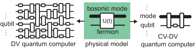
Figure 1: Digital hybrid oscillator-qubit circuits. Mapping a physical fermion-boson problem to an all-qubit (discrete variable, DV) circuit leads to large qubit and gate counts. Instead, we propose here to directly implement hybrid oscillator (continuous variable, CV)-qubit circuits.

This work is structured as follows. We start by reviewing elementary concepts (Sec. I). We then present our main results on compilation strategies. This is divided into fundamental primitives (Sec. II), methods for matter fields (Sec. III), and finally gauge-fields and their interactions with matter (Sec. IV). We then perform an end-to-end resource estimation of our methods and compare to all-qubit hardware (Sec. V). Finally, we introduce methods to measure observables, algorithms to perform dynamics simulation and ground-state preparation, and numerical benchmarks (Sec. VI), and conclude (Sec. VII).

As a guide to the reader, here is some more detail about each of the seven sections of this paper, in sequence. In Sec. I, i.e., the remainder of this introductory section, we give context by broadly introducing LGTs (Sec. I.1) and the challenges associated to their simulation. We choose paradigmatic models [23, 58] as a case study, the $\mathbb{Z}_{2}$-Higgs model and the $U(1)$ quantum link model, which we later use in Sec. VI to benchmark oscillator-qubit algorithms. We then introduce the superconducting hybrid oscillator-qubit hardware comprising transmon qubits coupled to high-Q microwave cavity resonators on which we base our study (Sec. I.2). Finally, we introduce Trotter algorithms (Sec. I.3), which are the basic subroutines used in our oscillator-qubit algorithms.

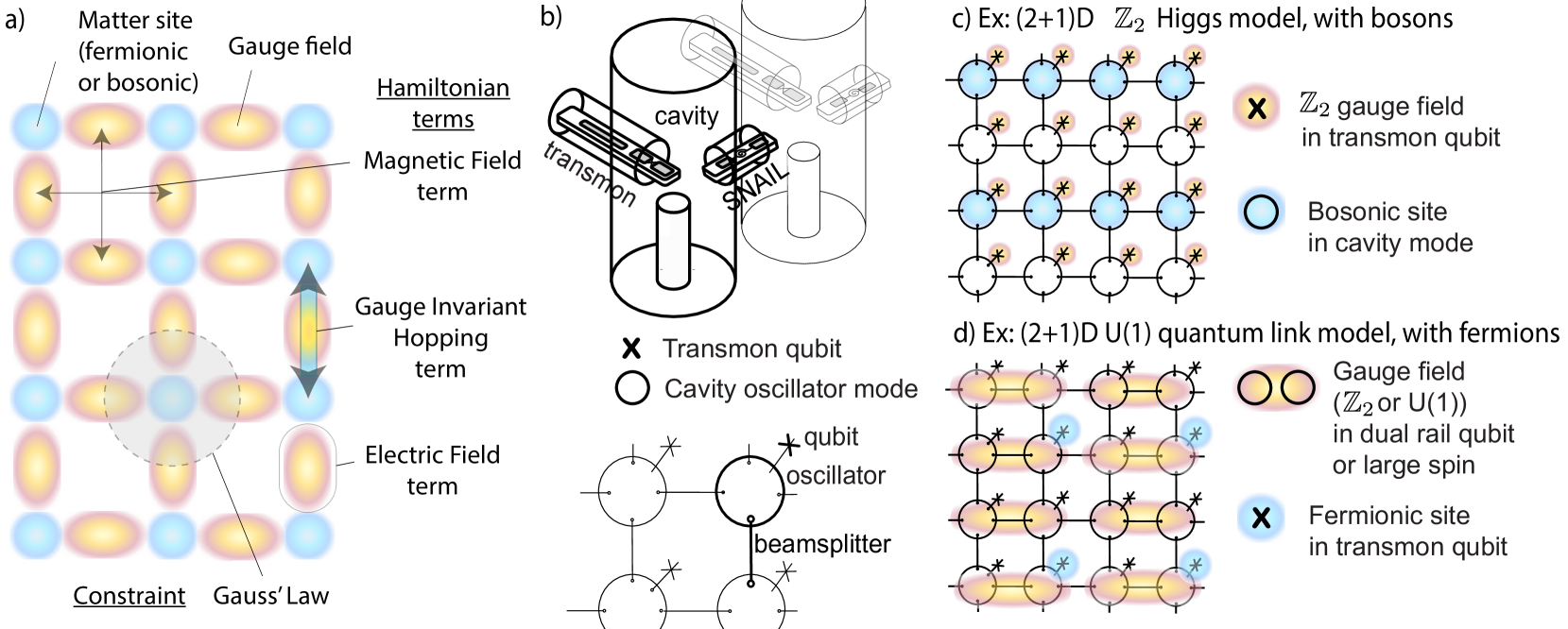
Figure 2: Mapping lattice gauge theory models to qubit and oscillator degrees of freedom in circuit QED. a) Lattice gauge theories. Components (Matter sites, Gauge field), Hamiltonian terms (gauge-invariant Hopping, Electric Field, Magnetic Field) and constraints (Gauss’s law) of lattice gauge theory models. b) Top: $3$D cavity architecture. Transmon qubits couple to the lowest-energy mode of the cavity by overlapping with the mode. SNAILs couple two cavities to each other. The cavities are approximately  $50$ mm long [59], with a diameter of approx. $10$ mm. Bottom: Corresponding schematic of an array of 3D cavities. Concentric circles represent cavities, implementing oscillators; crosses represent transmon qubits, implementing qubits; lines denote SNAILs used to implement beamsplitter operations between cavities. c) and d) Examples of models mapped to this architecture. c) $\mathbb{Z}_{2}$-Higgs model. The gauge fields are mapped to the transmon qubit degrees of freedom and there is one bosonic matter site per cavity, represented by one of the bosonic microwave modes in that cavity. d) $U(1)$ quantum link model. The gauge fields are mapped using the Schwinger-boson encoding to a pair of modes in two adjacent cavities, and the fermionic matter is mapped to transmon qubits. In $(2+1)$D, there are twice as many gauge field links as there are matter sites, which can be seen on the illustration. High fidelity $\operatorname{SWAP}$ operations between cavity modes enable the requested connectivity for this model.

In Sec. II, we introduce a toolset of hybrid oscillator-qubit compilation strategies used throughout this work. We review previously introduced methods, but also develop exact methods for synthesizing bosonic parity-dependent and density-density operations, as well as oscillator-mediated qubit-qubit entangling gates that we extend to multi-qubit gates.

In Sec. III we leverage this toolset to develop compilation strategies for implementing the time evolution operator for common bosonic (Sec. III.1) and fermionic (Sec. III.2) Hamiltonian terms, including single-site potentials, nearest-neighbor and onsite interactions, and hopping terms in hybrid superconducting hardware. We consider both $(1+1)$D and $(2+1)$D. For bosonic matter, we utilize the direct mapping of a bosonic matter site to a single mode of a microwave cavity. For fermionic matter, we leverage a Jordan-Wigner mapping using either transmon qubits or dual-rail qubits in microwave cavities.

In Sec. IV, we present compilation strategies for implementing pure gauge and gauge-matter Hamiltonian terms, specializing to the case of $\mathbb{Z}_{2}$ and $U(1)$ gauge fields in $(2+1)$D.

In Sec. V we introduce explicit Trotter circuits for the $\mathbb{Z}_{2}$-Higgs model and $U(1)$ quantum link model and perform an analysis of the Trotter errors. From this, we derive the end-to-end asymptotic scaling of the number of gates required for a dynamics simulation, including the errors encountered in the compilation. We then perform an explicit gate count comparison between our oscillator-qubit and an all-qubit simulation of the bosonic hopping Hamiltonian. To do so, we develop a qubit algorithm in the Fock-binary encoding to simulate bosonic hopping.

In Sec. VI, we adapt algorithms for ground-state preparation and dynamics to our oscillator-qubit approach, utilising the compilation methods from the previous sections. We use the $(1+1)$D $\mathbb{Z}_{2}$-Higgs model and $U(1)$ quantum link model as example models for numerical benchmarks using Bosonic Qiskit [60]. In particular, we develop an oscillator-qubit Variational Quantum Eigensolver (VQE) (Sec. VI.3, VI.4) ansatz. Within the VQE approach and in the context of the $\mathbb{Z}_{2}$-Higgs model model, we investigate the effects of hardware and shot noise on VQE ground-state preparation (Sec. VI.4) and demonstrate the utility of post-selection upon Gauss’ss law in improving ground state preparation. Following this, we show how to measure observables in these ground states, in particular non-local observables such as string order correlators and the superfluid stiffness (Sec. VI.5). Finally, we discuss ground state preparation with quantum signal processing (QSP) and compare the error in ground state preparation as a function of the time to solution between QSP and VQE (Sec. VI.6).

In Sec. VII we conclude with a summary of our main results, a discussion of the prospects for quantum advantage with our approach, and an outlook on some of the future research directions that are opened up by this work.

Before continuing, we briefly comment on vocabulary and notation used throughout this work. We will use the terms bosonic mode, qumode, oscillator, resonator, and cavity mode interchangeably. In general, we will refer to certain hybrid oscillator-qubit gates as being ‘controlled’ meaning that the generator of the gate contains either a qubit or a mode number-operator, i.e. the phase is proportional to the number of excitations in the state (the gate does nothing to $\ket{0}$). We generally call gates ‘conditioned’ when they obtain a state-dependent phase, i.e. the generator contains a qubit $\hat{Z}$ or mode Fock-state dependent phases, which could for example be implemented using a projector.

I.1 Lattice gauge theories

In the following, we briefly introduce the LGTs we will use as paradigmatic examples, a $\mathbb{Z}_{2}$-Higgs model and a $U(1)$ quantum link model, which we will show how to compile onto oscillator-qubit hardware in the rest of the study. Here, we introduce the Hamiltonian terms of these models in order to prepare our discussion on how to implement them. In Sec. VI.1, we will introduce their physics in the context of our numerical experiments, especially also emphasizing past work. Note that these models only serve as examples; due to the digital nature of our methods, our study enables the simulation of a wide range of models involving bosons, fermions and gauge fields.

In lattice gauge theories, matter fields reside on sites and gauge fields reside between sites, usually (for the case of 2+1-D) in a square lattice geometry.

$\mathbb{Z}_{2}$-Higgs model. In this model, the gauge fields are spin $1/2$ degrees of freedom. The Hamiltonian is written as follows [61, 62]:

$$\hat{H}_{\mathbb{Z}_{2}} =-g\sum_{\langle i,j\rangle}\hat{X}_{i,j}-B\sum_{i,j,k,l\in\square}\hat{Z}_{i,j}\hat{Z}_{j,k}\hat{Z}_{k,l}\hat{Z}_{l,i}$$

$$-J\sum_{\langle i,j\rangle}\left(\hat{m}^{\dagger}_{i}\hat{Z}_{i,j}\hat{m}_{j}+\mathrm{h.c.}\right)+U\sum_{i}\hat{n}_{i}^{2},$$ (1)

where $i,j$ indicates the link between lattice site $i$ and $j$ on a square lattice, $\sum_{\langle i,j\rangle}$ indicates a sum over all combinations of $i,j$ such that $i,j$ are nearest-neighbours and $\Box$ is a plaquette of four sites (see Fig. 2a). The annihilation operator at matter site $i$ is given by $\hat{m}_{i}$ and the density or occupation by $\hat{n}_{i}=\hat{m}^{\dagger}_{i}\hat{m}_{i}$. The matter can be either bosonic ($\hat{m}=\hat{a}$) or fermionic ($\hat{m}=\hat{c}$), with corresponding commutation/anticommutation relations $[\hat{a}_{i},\hat{a}_{j}^{\dagger}]=\delta_{ij}$ and $\{\hat{c}_{i},\hat{c}_{j}^{\dagger}\}=\delta_{ij}$. $\hat{X}_{i,j}$, $\hat{Z}_{i,j}$ are Pauli operators that act on the gauge field at the link between sites $i$ and $j$. The first, second, and third terms in Eq. (1) represent the electric field (coupling $g$), magnetic field (coupling $B$), and gauge-invariant hopping (coupling $J$), respectively. The last term is an on-site interaction of strength $U$ which is the simplest possible interaction term for bosonic matter, but does not contribute as an interaction term for (spinless) fermions since $\hat{n}^{2}=\hat{n}$, due to the Pauli exclusion principle.

The defining feature of gauge theories is invariance under local gauge transformations. This leads to the presence of Gauss’s law dividing up the Hilbert space of the theory into sectors which are not coupled by the Hamiltonian. This constraint is in analogy to the relation between the integral of the electric field flux through a surface and the charge enclosed by the surface in classical electrodynamics, with a product of field operators replacing the integral. $(-1)^{n_{i}}$ takes the role of the charge. In quantum mechanics, Gauss’s law is formulated as a constraint on the eigenstates $\ket{\Psi}$; for all $i$, $\hat{G}_{i}\ket{\psi}=q_{i}\ket{\psi}$, where $q_{i}\in\mathds{Z}$ and

$$\hat{G}_{i}=\prod_{\langle i,j\rangle}\hat{X}_{i,j}(-1)^{\hat{n}_{i}},$$ (2)

in $(2+1)$D, where the product is over the four links $\langle i,j\rangle$ that connect to site $i$, see Fig. 2a and c. We choose $q_{i}=1$ throughout this work. For open boundary conditions, terminated by matter sites, the Gauss’s law constraints on the boundary are fixed by imagining virtual qubit sites around the system and fixing them in a $\hat{X}$ product state. We set $\hat{X}=1$ for these qubits when necessary.

$U(1)$ quantum link model. The $U(1)$ LGT, which is equivalent to quantum electrodynamics in the limit of vanishing lattice spacing, hosts continuous gauge fields. The quantum link formalism [63, 64] replaces the gauge fields with discrete spin-$S$ degrees of freedom with commutation relations $[\hat{S}^{z}_{i},\hat{S}^{+}_{j}]=\delta_{ij}\hat{S}^{+}_{i}$ and $(\hat{S}^{z}_{i})^{2}+\frac{1}{2}\left(\hat{S}^{+}_{i}\hat{S}_{i}^{-}+\hat{S}^{-}_{i}\hat{S}_{i}^{+}\right)=S(S+1)$ [65, 66, 67, 68], where $S$ is the spin length leading to a Hilbert space cutoff of $2S+1$. The physics of continuous $U(1)$ gauge fields are recovered for $S\rightarrow\infty$ [69]. Choosing (large) finite $S$, this encoding approximately preserves the bosonic algebra. The Hamiltonian in this formalism reads [64]

$$\hat{H}_{U(1)} =\frac{g^{2}}{2}\sum_{\braket{i,j}}\left(\hat{S}^{z}_{i,j}+\frac{\tau}{2\pi}\right)^{2}$$

$$-\frac{1}{4g^{2}(S(S+1))^{2}}\sum_{i,j,k,l\in\square}\left(\hat{S}^{+}_{i,j}\hat{S}^{+}_{j,k}\hat{S}^{-}_{k,l}\hat{S}^{-}_{l,i}+\mathrm{h.c.}\right)$$

$$+\frac{J}{2\sqrt{S(S+1)}}\sum_{\braket{i,j}}\left(\hat{m}^{\dagger}_{i}\hat{S}^{+}_{i,j}\hat{m}_{j}+\mathrm{h.c.}\right)$$

$$+M\sum_{i}(-1)^{i}\hat{n}_{i},$$ (3)

where the first term is the electric field term, the second term is the magnetic field term, and the third is the gauge-invariant hopping. $g$ is the gauge-matter coupling strength and $J$ is the hopping strength. In one spatial dimension, the constant background electric field $\tau$ corresponds to a topological term [70, 71, 72, 73]. The last term is the staggered mass term with mass $M$, which comes from the mapping of the continuous Dirac fermion fields onto the lattice and is therefore only necessary for fermions [74]. We set the lattice spacing to unity here. Also note that in order to take the above Hamtiltonian to the continuum limit of QED, the phases in the hopping and staggered mass terms need to be slightly altered, c.f. [69]. This does not introduce any additional challenges in our implementation, so we choose the above convention for simplicity.

In addition, the physical states of the Hamiltonian, i.e. the gauge-invariant ones, have to fulfill Gauss’ss law: for all $\mathbf{i}$, $\hat{G}_{\mathbf{i}}\ket{\psi}=q_{\mathbf{i}}\ket{\psi}$, where $q_{\mathbf{i}}\in\mathds{Z}$ and

$$\hat{G}_{\mathbf{i}}=\hat{S}^{z}_{\mathbf{i}-\mathbf{e}_{x}}+\hat{S}^{z}_{\mathbf{i}-\mathbf{e}_{y}}-\hat{S}^{z}_{\mathbf{i}+\mathbf{e}_{x}}-\hat{S}^{z}_{\mathbf{i}+\mathbf{e}_{y}}-\hat{Q}_{\mathbf{i}}.$$ (4)

To clarify the spatial structure of Gauss’s law, we specify the lattice site as a two-dimensional vector $\mathbf{i}$ in this paragraph only. $\mathbf{e}_{x/y}$ is a unit vector in the $x/y$ direction of the lattice, respectively. In the above expression $\hat{Q}_{\mathbf{i}}=\hat{m}^{\dagger}_{\mathbf{i}}\hat{m}_{\mathbf{i}}-\left(1-(-1)^{r_{\mathbf{i}}}\right)/2$ is the staggered charge operator, where $r_{\mathbf{i}}$ is the Manhattan distance of the site $\mathbf{i}$ from the arbitrarily chosen origin. The fixed values $q_{\mathbf{i}}$ correspond to a choice of static background charge configuration, and for the rest of the paper we restrict ourselves to the sector of vanishing static charges, i.e., $q_{\mathbf{i}}=0$ for all $\mathbf{i}$.

In order to encode the spin $S$ degrees of freedom representing $U(1)$ gauge fields in the $U(1)$ quantum link model into bosonic modes, we use the Schwinger boson mapping. It consists of two bosonic modes, labelled $a$ and $b$, which fulfill the constraint $\hat{n}^{a}_{i,j}+\hat{n}^{b}_{i,j}=2S$. The electric field operator in this encoding is represented by

$$\hat{S}^{z}_{i,j}=\frac{\hat{n}^{a}_{i,j}-\hat{n}^{b}_{i,j}}{2},$$ (5)

and the electric field raising operator $S^{+}_{i,j}$ becomes

$$\hat{S}^{+}_{i,j} =\hat{a}^{\dagger}_{i,j}\hat{b}_{i,j}$$ (6)

$$\hat{S}^{-}_{i,j} =\hat{a}_{i,j}\hat{b}^{\dagger}_{i,j}$$ (7)

Compared to an encoding in just a single oscillator [75], our encoding allows for a smaller occupation of the modes to represent electric field zero, reducing the impact of mode decay.

We show a possible encoding of this model in our architecture in Fig. 2d.

I.2 Circuit QED platform

We now outline the main features of the platform we consider in the rest of the study – a lattice of microwave cavities coupled to superconducting transmon qubits (see Fig. 2b). In particular, we discuss the native Hamiltonian of this platform and the gates that can be implemented via microwave pulses.

Within the circuit QED framework, long-lived bosonic modes can be realized in three-dimensional superconducting microwave cavities with typical lifetimes on the order of one to ten milliseconds (ms) in aluminum [59, 76], Fig. 2a. Recently, niobium cavities have been used to improve coherence times, with observed single photon lifetimes on the order of $30$ ms [77] to over 1 s [78]. Separately, recent work realising planar microwave resonators, which may be more scalable due to their smaller size and fabrication advantages, have reached 1 ms single photon lifetimes [79]. In this platform, it is common to utilize one mode per cavity, although recent work has demonstrated that multi-mode cavities are also feasible [80].

Superconducting transmon qubits are routinely coupled to microwave cavities and used for control and readout via on-chip readout resonators [81]. The relaxation $T_{1}$ and dephasing times $T_{2}$ of transmons when coupled to microwave cavities are typically on the order of $250$ $\mu$s [82, 83, 84], with some recent coherence times in tantalum-based transmons reaching $500$ $\mu$s [85]. When simulating operation in hardware in section VI, we take into account the dominant source of hardware error, qubit decay and dephasing, adopting a conservative value of $T_{1}=T_{2}=200$ $\mu$s if not stated otherwise.

The SNAIL (Superconducting Nonlinear Asymmetric Inductive eLement) [86] is an attractive choice for realizing a programmable coupling between cavities. The SNAIL consists of three large junctions shunted by one small junction. When biased with a non-zero DC magnetic flux, the SNAIL (or SNAIL array) generates a three-wave mixing Hamiltonian that enables a parametrized beamsplitter interaction of strength $g(t)$ between the cavities while minimizing unwanted nonlinear static interactions, such as the cross-Kerr [87, 86, 88].

Our proposed architecture is an array of ‘oscillator-qubit pairs,’ each comprising a high-Q mode of a cavity dispersively coupled to a transmon qubit (see Fig. 2b, top panel). These units are arranged into a $2$D square lattice, where adjacent cavities are connected via a SNAIL, which can be used to implement a beamsplitter (see Fig. 2b, bottom panel). In the remainder of this work, we represent cavities (qubits) by circles (crosses). This symbolic representation will later prove useful for denoting the various possibilities for mapping systems of fermions, bosons and gauge fields onto this 2D hardware layout.

While this architecture is physically large in size (each cavity is about $50$ mm long [59]) and might therefore exhibit scaling limitations, planar resonators, while at present exhibiting shorter coherence times compared to 3D cavities, are smaller and therefore more scalable. Thus, the proposed architecture in Fig. 2b can also be implemented with planar resonators, and all results presented herein extend to this case (with the caveat that Hamiltonian parameters, loss rates and gate speeds are informed by recent experiments in 3D cavities, and would need to be adjusted to appropriately reflect the planar case).

Gate Name	Gate Operation
Mode gates
$\operatorname{R}_{i}(\theta)$	$\exp\left(-i\theta\hat{n}_{i}\right)$
$\operatorname{D}_{i}(\alpha)$	$\exp\left(\alpha\hat{a}_{i}^{\dagger}-\alpha^{*}\hat{a}_{i}\right)$
$\operatorname{BS}_{i,j}(\varphi,\theta)$	$\exp\left(-i\theta\left(e^{i\varphi}\hat{a}_{i}^{\dagger}\hat{a}_{j}+e^{-i\varphi}\hat{a}_{i}\hat{a}_{j}^{\dagger}\right)\right)$
Transmon gates
$\operatorname{R}_{i}^{z}(\theta)$	$\exp\left(-i\frac{\theta}{2}\hat{Z}_{i}\right)$
$\operatorname{R}_{i}^{\varphi}(\theta)$	$\exp\left(-i\frac{\theta}{2}\hat{\sigma}_{i}^{\varphi}\right)$ $\hat{\sigma}^{\varphi}_{i}=\hat{X}_{i}\cos\varphi+\hat{Y}_{i}\sin\varphi$
Transmon-Mode gates
$\operatorname{CR}_{i,j}(\theta)$	$\exp\left(-i\frac{\theta}{2}\hat{Z}_{i}\hat{n}_{j}\right)$
$\operatorname{C\Pi}_{i,j}$	$\exp\left(-i\frac{\pi}{2}\hat{Z}_{i}\hat{n}_{j}\right)$
$\operatorname{CD}_{i,j}(\alpha)$	$\exp\left(\hat{Z}_{i}\left(\alpha\hat{a}_{j}^{\dagger}-\alpha^{*}\hat{a}_{j}\right)\right)$
$\operatorname{SNAP}_{i,j}(\vec{\theta})$	$\exp\left(-i\hat{Z}_{i}\sum_{n}\theta_{n}\ket{n}\bra{n}_{j}\right)$
$\operatorname{SQR}_{i,j}(\vec{\theta},\vec{\varphi})$	$\sum_{n}\operatorname{R}^{\varphi_{n}}_{i}(\theta_{n})\otimes\ket{n}\bra{n}_{j}$

Table 1: Native transmon-mode gates. Note that transmon-mode gates are only native if $i=j$, i.e., both indices correspond to a directly coupled cavity-transmon pair. The case $i\neq j$ can be synthesized by combining native gates in sequence. Similarly, the beamsplitter is native if $i,j$ are nearest neighbors, i.e., the modes are directly coupled by a SNAIL, otherwise additional SWAP operations must be used. Note that $\operatorname{CR}_{i,i}(\chi_{i}t)$ corresponds to the ‘always on’ dispersive interaction between the $i$th cavity and transmon (though it can be effectively ‘turned off’ by echoing away its effects via dynamical decoupling – see discussion below). For the SNAP and SQR gates, $\ket{n}$ denotes the Fock state with occupation number $n$, fulfilling $\hat{n}\ket{n}=n\ket{n}$, while $\theta_{n}$ and $\varphi_{n}$ are the entries of the vectors $\vec{\theta}=\{\theta_{0},\theta_{1},\ldots\}$, $\vec{\varphi}=\{\varphi_{0},\varphi_{1},\ldots\}$. $\operatorname{CD}(\alpha)$ is a conditional displacement gate [89]. The parameter $\alpha$ is complex, while $\theta$ is real for all gates.

In this architecture, each transmon-cavity pair in the array is in the strong-dispersive coupling regime [81]. In the rotating-wave-approximation, the effective Hamiltonian of the 2D array can be written as:

$$\hat{H}=\hat{H}_{0}+\hat{H}_{1}$$ (8)

$$\hat{H}_{0}=\sum_{i=1}^{N}\frac{\chi_{i}}{2}\hat{Z}_{i}\hat{n}_{i}+\sum_{i=1}^{N}\left(\varepsilon_{i}(t)\hat{a}_{i}^{\dagger}+\Omega_{i}(t)\hat{\sigma}_{i}^{+}+\mathrm{h.c.}\right)$$ (9)

$$+\sum_{\braket{i,j}}\left(g_{i,j}(t)\hat{a}_{i}^{\dagger}\hat{a}_{j}+\mathrm{h.c.}\right)$$ (10)

$$\hat{H}_{1}=\sum_{i=1}^{N}K_{i}\hat{n}_{i}^{2}+\sum_{\braket{i,j}}\chi_{i,j}\hat{n}_{i}\hat{n}_{j}$$ (11)

Here, $\hat{a}_{i}$ ($\hat{a}_{i}^{\dagger}$) is the annihilation (creation) operator for the $i$th cavity mode, $\hat{n}_{i}=\hat{a}_{i}^{\dagger}\hat{a}_{i}$ is the corresponding number operator, and $\hat{\sigma}_{i}^{-}$ ($\hat{\sigma}_{i}^{+}$) is the lowering (raising) operator for the transmon coupled to the $i$th mode. $\hat{H}_{0}$ includes the dispersive shift ($\chi_{i}$), cavity drives ($\varepsilon_{i}(t)$), transmon Rabi drives ($\Omega_{i}(t)$), and tunable beamsplitter couplings ($g_{i,j}(t)$) implemented via SNAILs. The time-dependence in all parameters can be used to engineer different couplings. $\hat{H}_{1}$ includes additional unwanted static couplings such as self-Kerr ($K_{i}$) and cross-Kerr ($\chi_{i,j}$). These nonlinear couplings incur contributions from the hybridization of each cavity mode with the transmon and SNAIL couplers. With careful engineering, it is possible to design the components such that the Kerr contributions from transmon and SNAIL cancel or nearly cancel, and $\chi_{i,i+1}\approx 0$, $K_{i}\approx 0$ could be achieved at a single flux point, with small residual couplings not likely to contribute to the principal results of this work [86]. When the beamsplitter interaction is not activated ($g_{i,j}=0$), each oscillator-qubit pair can be independently controlled. For a full discussion of the gates available in the proposed superconducting hybrid oscillator-qubit platform, see Ref. [45]. The native gates arising directly from the Hamiltonian of the system are collected in Tab. 1. Note that in some parameter regimes, certain transmon-conditioned bosonic operations, such as the conditional displacement (sometimes referred to as ‘controlled displacement’) [89], can be implemented natively.

All phase-space rotations $\mathrm{R}_{i}\left(\theta\right)$ can be realized ‘in software’ by absorbing them into the phases of the subsequent microwave pulses. This is because all operations are carried out in the rotating frame of the free evolution of the cavity oscillator mode $\omega\hat{a}^{\dagger}\hat{a}$ (each transmon is only ever connected to a single cavity). Therefore, a phase-space rotation can be applied by changing the phase of the subsequent microwave drive carrying out a gate (such as a beamsplitter or displacement) on the corresponding mode. Arbitrary qubit $Z$ rotation gates can similarly be carried out in software.

Arbitrary initial states for each cavity can be prepared using optimal control [89, 90]: both qubit and cavity are initialised to the ground state, the qubit prepares the cavity in the required Fock state and is then measured to validate this preparation [91]. In particular, Fock states $\ket{n}$ with low photon number can be prepared with typical state-of-the-art Fock preparation infidelities of 10^-2 [91, 92, 93].

As mentioned above, it is possible to effectively turn off the ‘always on’ dispersive interaction using dynamical decoupling. Specifically, the transmons can be driven with Rabi rate $\Omega_{i}\gg\chi_{i}\braket{\hat{a}_{i}^{\dagger}\hat{a}_{i}}$ during a time $T=2\pi k/\Omega_{i}$, where $k$ is an integer, to decouple the cavity mode from the transmon and leave the transmons in their initial state. With this, the beamsplitter gate $\text{BS}_{i,j}(\varphi,\theta)$ is performed by simultaneously driving transmons $i$ and $j$, and driving the SNAIL coupler linking modes $i$ and $j$ such that $g_{i,j}>0$. Alternative schemes based on transmon echoing can also be used to decouple and perform transmon-state-independent beamsplitting [94].

In addition to unitary control, the transmons can be leveraged for measurements of the cavity modes. In particular, it is possible to measure the boson occupation in the mode in a total duration that is logarithmic in the maximum Fock state. This is done by reading out the photon number bit-by-bit in its binary representation. Each bit is mapped onto the transmon qubit dispersively coupled to the cavity, which is measured and then reset  [95, 96].

I.3 Trotter simulations

In this work, we focus on a Trotter decomposition of dynamics as our basic simulation algorithm. In such simulations, the time evolution operator $\exp\left(-i\hat{H}T\right)$ until time $T$ with Hamiltonian $\hat{H}=\sum_{\gamma=1}^{\Gamma}\hat{H}_{\gamma}$ is divided into $r$ time steps of duration $t=T/r$, i.e., $\exp\left(-i\hat{H}T\right)=\left(\exp\left(-i\hat{H}t\right)\right)^{r}$. If $t$ is chosen sufficiently small, a product formula approximation to $\exp\left(-i\hat{H}t\right)$ can then be employed to decompose the Hamiltonian into unitaries which only act on a few qubits and oscillator modes. For example, a $(2p)^{\rm th}$-order Trotter formula in general can be written as a sequence of $N_{\exp}$ exponentials of Hamiltonian terms $\hat{H}_{\gamma_{i}}$ drawn from $\{\hat{H}_{1},\ldots,\hat{H}_{\Gamma}\}$ and a sequence of times $t_{i}$ with $|t_{i}|\leq t$ that satisfies

$$\exp\left(-i\hat{H}t\right)=e^{-i\hat{H}_{\gamma_{1}}t_{1}}\cdots e^{-i\hat{H}_{\gamma_{N_{\exp}}}t_{N_{\exp}}}+\mathcal{O}(t^{2p+1}).$$ (12)

There is great freedom in the choice of this decomposition; however, certain orderings can be cheaper, more accurate or more natural. We choose our decomposition to be given by the local terms inside the sums over lattice sites in many-body Hamiltonians, c.f. Eq. (1) and Eq. (3). For example, the first-order Trotter decomposition of the $\mathbb{Z}_{2}$-Higgs model for $U=0$ in one spatial dimension, where $B=0$, is given by

$$e^{-i\hat{H}_{\mathbb{Z}_{2}}t}=\prod_{\langle i,j\rangle}e^{igt\hat{X}_{i,j}}\prod_{\langle i,j\rangle}e^{iJt\left(\hat{m}^{\dagger}_{i}\hat{Z}_{i,j}\hat{m}_{j}+\mathrm{h.c.}\right)}+\mathcal{O}(t^{2}).$$ (13)

One of the main goals of this paper is to show how to compile unitaries acting on two or more sites, such as the gauge-invariant hopping $\exp{\left[iJt\left(\hat{m}^{\dagger}_{i}\hat{Z}_{i,j}\hat{m}_{j}+\mathrm{h.c.}\right)\right]}$, into the native operations available in circuit QED hardware or other hardware with equivalent instruction set architectures.

In section V, we discuss the errors incurred from the Trotter approximation and their interplay with compilation errors.

II Implementation primitives

In this section, we introduce the key compilation strategies we use to synthesize oscillator-oscillator, qubit-qubit, and oscillator-qubit gates from native operations. Throughout, we use the word “qubit” to refer either to a transmon qubit or a dual-rail qubit encoded in two cavities [97, 98, 99, 100, 91, 101], and only distinguish between the two possibilities when clarification is necessary. A summary of the gates we obtain through these compilation strategies is provided in Tab. 2. These primitives will then be used in Sections III and IV to compile Hamiltonian terms comprising fermions, bosons, and gauge-fields to native operations.

Gate	Definition	Gate Decomposition	Reference
$\operatorname{SWAP}_{i,j}$	$\sum_{n,m}\ket{m}\bra{n}_{i}\otimes\ket{n}\bra{m}_{j}$	$\operatorname{R}_{i}(\frac{\pi}{2})\operatorname{R}_{j}(\frac{\pi}{2})\textrm{BS}_{i,j}\left(0,\frac{\pi}{2}\right)$	Sec. II.1
$\operatorname{CU}^{Z}_{i,j}$	$\exp{\left(\hat{Z}_{i}\left(\hat{\Theta}\hat{a}_{j}^{\dagger}-\hat{\Theta}^{\dagger}\hat{a}_{j}\right)\right)}$	$\operatorname{C\Pi}_{i,j}e^{i\left(\hat{\Theta}\hat{a}_{j}^{\dagger}+\hat{\Theta}^{\dagger}\hat{a}_{j}\right)}\operatorname{C\Pi}_{i,j}^{\dagger}$	Fig. 3, Sec. II.2
$\operatorname{CU}^{P}_{i,j}$	$\exp{\left(-i\hat{Z}_{\textrm{anc}}\hat{P}_{i}\hat{O}_{j}\right)}$	$\operatorname{SQR}_{\textrm{anc},i}(\vec{\theta}_{P},\vec{0})e^{-i\hat{Z}_{\textrm{anc}}\hat{O}_{j}}\operatorname{SQR}_{\textrm{anc},i}(-\vec{\theta}_{P},\vec{0})$	Sec. II.3
$\operatorname{CU}^{\hat{n}}_{i,j}$	$\exp{(-i\hat{Z}_{\textrm{anc}}\hat{n}_{i}\hat{O}_{j})}$	$\prod_{k=0}^{K-1}\operatorname{SQR}_{\textrm{anc},i}(\vec{\pi}_{k},\vec{0})e^{-i2^{k-1}\hat{O}_{j}}e^{i2^{k-1}\hat{Z}_{\textrm{anc}}\hat{O}_{j}}\operatorname{SQR}_{\textrm{anc},i}(-\vec{\pi}_{k},\vec{0})$	Fig. 4, Sec. II.5
$\operatorname{RR}_{i,j}(\theta)$	$\exp{\left(-i\theta\hat{Z}_{\textrm{anc}}\hat{n}_{i}\hat{n}_{j}\right)}$	$\prod_{k=0}^{K-1}\operatorname{SQR}_{\textrm{anc},i}(\vec{\pi}_{k},\vec{0})\operatorname{R}_{j}\left(\frac{2^{k}\theta}{2}\right)\operatorname{CR}^{\dagger}_{i,j}\left(\frac{2^{k}\theta}{2}\right)\operatorname{SQR}_{\textrm{anc},i}(-\vec{\pi}_{k},\vec{0})$	Sec. II.5
$\operatorname{ZZ}_{i,j}(\theta)$	$\exp\left(-i\frac{\theta}{2}\hat{Z}_{i}\hat{Z}_{j}\right)$	$\textrm{CD}_{i,j}(-i\sqrt{\theta}/2)\textrm{CD}_{i,i}(\sqrt{\theta}/2)\textrm{CD}_{i,j}(+i\sqrt{\theta}/2)\textrm{CD}_{i,i}(-\sqrt{\theta}/2)$	Fig. 5, Sec. II.6
BCH	$\exp\left(-2i\hat{Z}\hat{O}_{\vec{I}}\hat{O}_{\vec{J}}\theta^{2}\right)$	$\operatorname{CU}^{X}_{k,\vec{I}}(\theta)\operatorname{CU}^{Y}_{k,\vec{J}}(\theta)\operatorname{CU}^{X}_{k,\vec{I}}(-\theta)\operatorname{CU}^{Y}_{k,\vec{J}}(-\theta)+\mathcal{O}(\theta^{3})$	Fig. 6, Sec. II.7
Trotter	$\exp{\left(-i\hat{Z}\left(\hat{O}_{\vec{I}}+\hat{O}_{\vec{J}}\right)\theta\right)}$	$\operatorname{CU}_{i,\vec{I}}^{Z}(\theta)\operatorname{CU}^{Z}_{j,\vec{J}}(\theta)+\mathcal{O}(\theta^{2})$	Fig. 6, Sec. II.7

Table 2: Non-native primitives used in this study and section references where their synthesis is explained. Row 2) $\operatorname{CU}^{Z}$ is a qubit-conditional variant of the unitary $\hat{U}=\textrm{exp}(\hat{\Theta}\hat{a}_{j}^{\dagger}-\hat{\Theta}^{\dagger}\hat{a}_{j})$, where $\hat{\Theta}$ is any operator that commutes with $\hat{a}_{j}$ and $\hat{Z}_{j}$. For example, $\hat{\Theta}\to\alpha$ corresponds to a conditional displacement (see Eq. (18)), while $\hat{\Theta}\to\theta e^{i\varphi}\hat{a}_{k}$ yields a conditional beamsplitter (see Eq. (19)). Row 3) An ancilla-mediated variant of the unitary $\hat{U}=\textrm{exp}(-i\hat{O}_{j})$ on mode $j$ that is conditioned by an operator $\hat{P}_{i}$ on mode $i$. Here, $\hat{P}_{i}$ can be any operator that is diagonal in Fock-space with eigenvalues $\pm 1$. The angles $\vec{\theta}_{P}$ are chosen according to Eq. (32). Row 4) An ancilla-mediated variant of $\hat{U}=\textrm{exp}(-i\hat{O}_{j})$ conditioned on the photon number $\hat{n}_{i}$ of mode $i$. This leverages an iterative sequence of the primitive $\operatorname{CU}_{i,j}^{P}$ with the $k$th iteration conditioning on the $k$th bit of $\hat{n}_{i}$, requiring $K=\lceil\log_{2}(n_{\mathrm{max}}+1)\rceil$ total iterations where $n_{\mathrm{max}}$ is the maximum photon-number cutoff for mode $i$. Row 5) A useful instance of $\operatorname{CU}_{i,j}^{\hat{n}}$ where $\hat{O}_{j}\to\theta\hat{n}_{j}$. $\vec{\pi}_{k}$ is defined in Eq. (41). Row 6) An example of an oscillator-mediated entangling gate between two transmons. Rows 7 & 8) Approximate methods, see relevant sections for discussion and Ref. [102] for the BCH method. The superscripts $X$ and $Y$ in $\operatorname{CU}$ denote the qubit axis on which the operator $\hat{U}$ is conditioned. This axis can be controlled by conjugating $\operatorname{CU}^{Z}$ by single qubit rotations. $\vec{I}$ and $\vec{J}$ indicate support on a vector of mode indices.

Specifically, in Sec. II.1, we discuss the bosonic SWAP gate, a particularly useful primitive that enables the synthesis of entangling gates between non-neighbouring modes. In Sec. II.2, we demonstrate how one can synthesize qubit-conditioned bosonic operations using conditional parity gates and, in Sections II.3 and II.4, develop strategies to realize bosonic operations conditioned or controlled on the Fock-space occupancy of another mode. Building upon these “Fock-projector-conditioned” and “Fock-projector-controlled” operations, we then discuss how one can apply them in sequence to implement more complex density-controlled gates in Sec. II.5. We then discuss a technique for implementing oscillator-mediated, multi-qubit gates in Sec. II.6, and follow this with a discussion on approximate methods for synthesizing multi-mode gates in Sec. II.7. Finally, we discuss the dual-rail encoding in Sec. II.8 as an alternative scheme for realizing qubits in the proposed hybrid oscillator-qubit architecture.

II.1 Bosonic SWAP

Our architecture in Fig. 2 is not all-to-all connecting, and hence it is useful to be able to implement SWAP operations between the bosonic sites. In particular, bosonic SWAP gates enable quantum communication and entangling operations between remote bosonic modes, and additionally allow for entangling operations between qubits using the bosonic modes as a quantum bus [45].

To that end, a bosonic SWAP gate can be realized using a beamsplitter and a pair of phase-space rotations,

$$\operatorname{SWAP}_{i,j}=\operatorname{R}_{i}\left(-\frac{\pi}{2}\right)\operatorname{R}_{j}\left(-\frac{\pi}{2}\right)\textrm{BS}_{i,j}\left(0,\frac{\pi}{2}\right).$$ (14)

with $\operatorname{BS}_{i,j}(\varphi,\theta)$ and $\operatorname{R}_{j}\left(\theta\right)$ defined in Tab. 1. Here, the role of the phase-space rotations is to cancel the spurious phase obtained from the action of the beamsplitter, $\operatorname{BS}_{i,j}(0,\frac{\pi}{2})\left|\Psi_{i},\Psi_{j}\right\rangle=e^{-i\frac{\pi}{2}\left[\hat{n}_{i}+\hat{n}_{j}\right]}\left|\Psi_{j},\Psi_{i}\right\rangle$. As mentioned previously, all such phase-space rotations $\operatorname{R}_{i}\left(\theta\right)$ can be realized ‘in software’ by absorbing them into the phases of the subsequent microwave drives. In the proposed architecture with SNAILs linking adjacent cavities, SWAP operations have been demonstrated with a duration of around 100 ns and a fidelity of $\sim 0.999$ [103, 86].

As discussed in Sec. I.2, our proposed architecture assumes native entangling gates between each mode-qubit pair and beamsplitters are only available between adjacent sites. However, as discussed in Ref. [45], it is possible to use a beamsplitter network (i.e., a sequence of bosonic SWAPs) to synthesize non-native oscillator-oscillator and oscillator-qubit gates, e.g., $\operatorname{BS}_{i,j}(\varphi,\theta)$ for any modes $i\neq j$, and $\operatorname{CR}_{i,j}(\theta)$ for any transmon $i$ and mode $j$. Thus, we will henceforth assume access to such non-native gates, abstracting away the underlying bosonic SWAPs.

II.2 Qubit-conditioned bosonic operations

Certain bosonic operations, such as beamsplitters or displacements, can be conditioned on qubits by conjugating them with conditional parity gates, $\operatorname{C\Pi}_{i,j}$ [45]. The intuition for this is provided by the relation

$$\operatorname{C\Pi}_{i,j}\hat{a}_{j}\operatorname{C\Pi}^{\dagger}_{i,j}=i\hat{Z}_{i}\hat{a}_{j},$$ (15)

where we used the Baker-Campbell-Hausdorff formula

$$e^{\hat{A}}\hat{B}e^{-\hat{A}}=\hat{B}+[\hat{A},\hat{B}]+\frac{1}{2!}[\hat{A},[\hat{A},\hat{B}]]+\ldots,$$ (16)

and $\operatorname{C\Pi}_{i,j}$ is the conditional parity gate defined in Tab. 1, experimentally realized by evolving under the dispersive interaction for a time $T=\pi/\chi$ (see Eq. (9)).

It is possible to implement the Hermitian adjoint $\operatorname{C\Pi}_{i,j}^{\dagger}$ by simply appending a bosonic phase-space rotation:

$$\operatorname{C\Pi}_{i,j}^{\dagger} =\operatorname{R}_{j}(-\pi)\operatorname{C\Pi}_{i,j}=\operatorname{C\Pi}_{i,j}\operatorname{R}_{j}(-\pi).$$ (17)

This is because $\operatorname{C\Pi}_{i,j}^{\dagger}=e^{i\frac{\pi}{2}\hat{Z}_{i}\hat{n}_{j}}=e^{i\pi\hat{Z}_{i}\hat{n}_{j}}e^{-i\frac{\pi}{2}\hat{Z}_{i}\hat{n}_{j}}$, and $e^{i\pi\hat{Z}_{i}\hat{n}_{j}}=\cos(\pi\hat{n})\mathds{1}+i\sin(\pi\hat{n})\hat{Z}=\cos(\pi\hat{n})=e^{i\pi\hat{n}_{j}}$. In effect, applying a $\operatorname{C\Pi}_{i,j}^{\dagger}$ gate requires the application of $\operatorname{C\Pi}_{i,j}$ and a phase-space rotation $\operatorname{R}_{j}(-\pi)=\operatorname{R}_{j}(\pi)$ which, as explained in Sec. I.2, can be implemented ‘in software’ via modification of the phases of the subsequent microwave drives.

The relation in Eq. (15) allows us to “convert” the generator of certain bosonic operations into one that depends upon the state of a qubit. For example, the conditional displacement gate can be synthesized from an unconditional displacement and a pair of conditional parity gates via

$$\operatorname{CD}_{i,j}(\alpha) =e^{\hat{Z}_{i}\left(\alpha\hat{a}_{j}^{\dagger}-\alpha^{*}\hat{a}_{j}\right)}$$ (18)

$$=e^{-i\frac{\pi}{2}\hat{Z}_{i}\hat{n}_{j}}e^{i\left(\alpha\hat{a}_{j}^{\dagger}+\alpha^{*}\hat{a}_{j}\right)}e^{i\frac{\pi}{2}\hat{Z}_{i}\hat{n}_{j}}$$

$$=\operatorname{C\Pi}_{i,j}\operatorname{D}_{i}(i\alpha)\operatorname{C\Pi}_{i,j}^{\dagger},$$

where $\alpha\in\mathds{C}$. Note the modified phase in the unconditional displacement. This is due to the factor of $i$ inherited from the transformation in Eq. (1). Furthermore, we emphasize that while this sequence produces exactly the conditional displacement gate as defined in Table 1, this gate can more efficiently be realized natively using the techniques developed in Ref. [89].

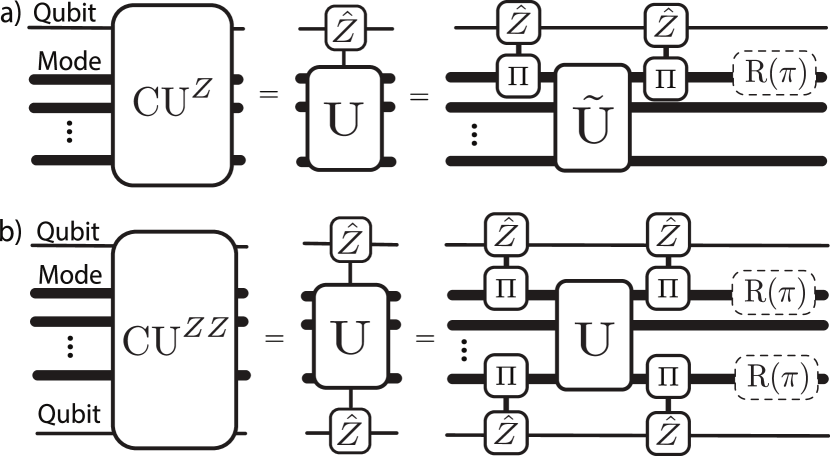
Figure 3: Qubit-conditional bosonic gates. Circuit diagrams containing qubits (thin line) and modes (thick lines), with time going from left to right. All conditional gates represent unitaries conditional on $\hat{Z}$. a) Qubit-conditional gate of the form $\operatorname{CU}^{Z}_{i,j}$ defined in Eq. (20). Here, $\operatorname{\tilde{U}}$ denotes the unconditional variant of $\textrm{CU}^{Z}$. The tilde indicates that the phase is modified by $\pi/2$ – see, e.g., Eq. (18). Gates with dashed box can be implemented ‘in software’ as explained in Sec. I.2. b) Multi-controlled bosonic operations, implemented by repeating the primitive in panel a), see Eq. (21).

As another example, we can exactly compile the conditional beamsplitter gate as follows:

$$\text{CBS}_{i,j,k}(\varphi,\theta) =e^{-i\theta\hat{Z}_{i}\left(e^{i\varphi}\hat{a}^{\dagger}_{j}\hat{a}_{k}+e^{-i\varphi}\hat{a}_{j}\hat{a}^{\dagger}_{k}\right)},$$ (19)

$$=e^{-i\frac{\pi}{2}\hat{Z}_{i}\hat{n}_{j}}e^{\theta\left(e^{i\varphi}\hat{a}^{\dagger}_{j}\hat{a}_{k}-e^{-i\varphi}\hat{a}_{j}\hat{a}^{\dagger}_{k}\right)}e^{i\frac{\pi}{2}\hat{Z}_{i}\hat{n}_{j}}$$

$$=\operatorname{C\Pi}_{i,j}\,\text{BS}_{j,k}(\varphi+\pi/2,\theta)\operatorname{C\Pi}_{i,j}^{\dagger},$$

where $\{\varphi,\theta\}\in\mathds{R}$. This gate will play an instrumental role in Sec. IV for the compilation of interaction terms between matter and gauge fields. Its duration is experimentally limited by the speed of each conditional parity gate, requiring roughly $1$ $\mu$s each. As such, the conditional beamsplitter gate requires $\sim 2.1$ $\mu$s, including the worst-case $\sim 100$ ns required for a full SWAP beamsplitter [103].

More generally, as shown in Fig. 3a, we can employ this strategy to realize a conditional unitary $\operatorname{CU}^{Z}_{i,j}$ from its unconditional counterpart:

$$\begin{split}\operatorname{CU}^{Z}_{i,j}&=e^{\hat{Z}_{i}\left(\hat{\Theta}\hat{a}^{\dagger}_{j}-\hat{\Theta}^{\dagger}\hat{a}_{j}\right)}\\ &=\operatorname{C\Pi}_{i,j}e^{i\left(\hat{\Theta}\hat{a}_{j}^{\dagger}+\hat{\Theta}^{\dagger}\hat{a}_{j}\right)}\operatorname{C\Pi}_{i,j}^{\dagger}.\end{split}$$ (20)

This decomposition holds for any choice of operator $\hat{\Theta}$ that satisfies $[\hat{\Theta},\hat{a}_{j}]=[\hat{\Theta},\hat{Z}_{i}]=0$. For instance, $\hat{\Theta}\to\alpha$, corresponds to the conditional displacement in Eq. (18) while $\hat{\Theta}\to\theta e^{i\varphi}\hat{a}_{k}$ yields the condition beamsplitter in Eq. (19).

This strategy can be iterated to realize bosonic gates conditioned on multiple qubits. For example, one can realize a doubly-conditioned gate of the form

$$\operatorname{CU}^{ZZ}_{i,j,k}=e^{\hat{Z}_{i}\hat{Z}_{j}\left(\hat{\Theta}\hat{a}_{k}^{\dagger}-\hat{\Theta}^{\dagger}\hat{a}_{k}\right)}$$ (21)

for any operator $\hat{\Theta}$ that commutes with $\hat{Z}_{i}$, $\hat{Z}_{j}$, and $\hat{a}_{k}$. In this case, conditional parity gates are implemented on mode $k$ for qubits $j$ and $k$ in sequence with the aid of SWAP gates. Alternatively, one can apply conditional parity gates acting on different qubit-mode pairs in parallel as shown in Fig. 3b.

We note that, in the above, we use ‘qubit-conditional’ and ‘qubit-controlled’ interchangeably to refer to a gate that enacts a bosonic operation that depends upon the $Z$ basis state of a qubit. In particular, distinct non-trivial operations are enacted for both qubit state $\ket{0}$ and $\ket{1}$. However, in certain contexts, it is useful to synthesize a ‘$1$-controlled’ bosonic operation, i.e., one that acts only if the qubit is in $\ket{1}$. In this work, we will refer to this as an $n$-controlled gate, referring to the operator that appears as a multiplicative factor in the generator. For example, for an $n$-controlled mode rotation, we have

$$e^{-i\theta\hat{n}_{\mathrm{qubit}}\hat{n}_{\mathrm{mode}}}=\operatorname{R}_{i}\left(-\frac{\theta}{2}\right)\operatorname{CR}_{i,i}(\theta),$$ (22)

where $\hat{n}_{\mathrm{qubit}}=(\mathds{1}-\hat{Z})/2$. More generally, we have

$$e^{i\theta\hat{n}_{\mathrm{qubit}}\hat{O}_{i}}=e^{i\frac{\theta}{2}\hat{O}_{i}}e^{-i\frac{\theta}{2}\hat{Z}_{i}\hat{O}_{i}},$$ (23)

for any $\hat{O}_{i}$ which commutes with operations on the qubit.

II.3 Fock-projector-conditioned bosonic operations

An important primitive in the hybrid oscillator-qubit architecture of Fig. 2 is the synthesis of nontrivial two-mode entangling gates. In this section, we develop a technique to realize bosonic operators that are conditioned on the Fock-space information of a second mode:

$$\operatorname{CU}_{i,j}^{\bar{P}}=e^{-i\hat{Z}_{\textrm{anc}}\bar{P}_{i}\hat{O}_{j}},$$ (24)

where $\bar{P}_{i}$ is an operator with eigenvalues $\pm 1$ defined below (hence the name ‘conditioned’), ‘anc’ refers to an ancillary transmon qubit and $\hat{O}_{j}$ is an arbitrary (Hermitian) operation acting on mode $j$. For an arbitrary subspace $\mathcal{P}$ of the oscillator, $\bar{P}_{i}$ gives states inside $\mathcal{P}$ a phase of $-1$, and states outside $\mathcal{P}$ a phase of $1$. Mathematically,

$$\bar{P}_{i} =\sum_{n\notin\mathcal{P}}\ket{n}\bra{n}_{i}-\sum_{n\in\mathcal{P}}\ket{n}\bra{n}_{i},$$ (25)

where each projector acts on mode $i$. Note that we define the operator $\bar{P}_{i}$ without a hat for simplicity of notation.

Because $\bar{P}_{i}$ has eigenvalues $\pm 1$, the core idea is to map this information to an ancillary qubit, which is then used to mediate this information to a second mode via a hybrid qubit-mode gate. This effectively realises the Fock-projector-conditioned bosonic gate in Eq. (24). This requires the ancillary qubit to be initialized to an eigenstate of $\hat{Z}_{\textrm{anc}}$. This ancillary qubit can correspond to the transmon qubit dispersively coupled to mode $i$ or $j$, or any other qubit via appropriate use of bosonic SWAP gates.

To explain further, we begin with the particular example of a parity-conditioned gate, defined as

$$\operatorname{CU}^{\bar{\Pi}}_{i,j} =e^{-i\hat{Z}_{\textrm{anc}}\bar{\Pi}_{i}\hat{O}_{j}},$$ (26)

where

$$\bar{\Pi}_{i} =e^{i\pi\hat{n}_{i}}$$ (27)

is the parity operator acting on mode $i$ with eigenvalues $\pm 1$. Therefore, for an ancilla initialized to $\ket{0}_{\textrm{anc}}$, $\operatorname{CU}^{\bar{\Pi}}_{i,j}$ applies the unitary $e^{-i\hat{O}_{j}}$ ($e^{i\hat{O}_{j}}$) to mode $j$ if mode $i$ has even (odd) parity. To realize this gate, it is helpful to first note that

$$\textrm{SQR}_{\textrm{anc},i}(\vec{\pi}_{0},\vec{0})=e^{-i\frac{\pi}{2}\hat{X}_{\textrm{anc}}\sum_{n\textrm{ odd}}\ket{n}\bra{n}_{i}},$$ (28)

where $\vec{\pi}_{0}=\{0,\pi,0,\pi,\ldots\}$ and $\vec{0}=\{0,0,0,\ldots\}$, and $\hat{\Pi}_{i}$ (as opposed to $\bar{\Pi}_{i}$) is the projector over odd Fock states. In other words, an SQR gate is simply a Fock-projector-controlled qubit rotation. By leveraging the Baker-Cambell-Hausdorff formula in Eq. (16), it can be shown that

$$\textrm{SQR}_{\textrm{anc},i}(\vec{\pi}_{0},\vec{0})\hat{Z}_{\textrm{anc}}\textrm{SQR}^{\dagger}_{\textrm{anc},i}(\vec{\pi}_{0},\vec{0})=\hat{Z}_{\textrm{anc}}\bar{\Pi}_{i}.$$ (29)

Thus, in direct analogy to the strategy for synthesizing qubit-conditional bosonic operations in Sec. II.2, we can leverage a pair of SQR gates to condition a bosonic operation on the parity of a second mode:

$$\operatorname{CU}^{\bar{\Pi}}_{i,j}=\textrm{SQR}_{\textrm{anc},i}(\vec{\pi}_{0},\vec{0})e^{-i\hat{Z}_{\textrm{anc}}\hat{O}_{j}}\textrm{SQR}_{\textrm{anc},i}(-\vec{\pi}_{0},\vec{0}),$$ (30)

where we have used the fact that $\textrm{SQR}^{\dagger}_{\textrm{anc},i}(\vec{\theta},\vec{\varphi})$ = $\textrm{SQR}_{\textrm{anc},i}(-\vec{\theta},\vec{\varphi})$. This requires the realization of the intermediary qubit-oscillator gate $\exp(-i\hat{Z}_{\textrm{anc}}\hat{O}_{j})$, either natively or, e.g., using the technique in Sec. II.2.

Returning to the general form in Eq. (24), it is possible to generalize this technique by substituting $\bar{\Pi}_{i}$ with $\bar{P}_{i}$ which allows for any arbitrary set of Fock states $\mathcal{P}$ by choosing appropriate angles for the SQR gate in Eq. (30). In particular, Eq. (29) generalizes as

$$\textrm{SQR}_{\textrm{anc},i}(\vec{\theta}_{P},\vec{0})\hat{Z}_{\textrm{anc}}\textrm{SQR}^{\dagger}_{\textrm{anc},i}(\vec{\theta}_{P},\vec{0})=\hat{Z}_{\textrm{anc}}\bar{P}_{i},$$ (31)

where $\vec{\theta}_{P}=\{\theta_{0},\theta_{1},\ldots,\theta_{n}\,\ldots\}$ and

$$\theta_{n}=\begin{cases}\pi&\text{if $\ket{n}\in\mathcal{P}$}\\ 0&\text{otherwise}.\end{cases}$$ (32)

Akin to Eq. (28), this leverages the fact that $\operatorname{SQR}_{\textrm{anc},i}(\vec{\theta}_{P},\vec{0})$ realizes a projector-controlled qubit rotation:

$$\textrm{SQR}_{\textrm{anc},i}(\vec{\theta}_{P},\vec{0})=e^{-i\frac{\pi}{2}\hat{X}_{\textrm{anc}}\sum_{n\in\mathcal{P}}\ket{n}\bra{n}_{i}}.$$ (33)

Thus, with this, one can realize the generalized Fock-projector-conditional gate,

$$\begin{split}\operatorname{CU}_{i,j}^{\bar{P}}&=e^{-i\hat{Z}_{\textrm{anc}}\bar{P}_{i}\hat{O}_{j}}\\ &=\textrm{SQR}_{\textrm{anc},i}(\vec{\theta}_{P},\vec{0})e^{-i\hat{Z}_{\textrm{anc}}\hat{O}_{j}}\textrm{SQR}_{\textrm{anc},i}(-\vec{\theta}_{P},\vec{0}).\end{split}$$ (34)

This sequence is illustrated in Fig. 4a.

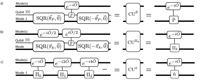
Figure 4: Mode-conditioned and controlled unitaries a) Bosonic Fock-projector-conditioned unitary, see Eq. (34). b) Bosonic parity-controlled unitary. c) Compilation of a bosonic controlled, or occupation-controlled unitary, by binary phase acquisition (cf Eq. (39)). The upper mode denoted by ’mode(s)’ may contain any set of modes or qubits for which $e^{-i\hat{O}}$ commutes with the lower qubit and mode on which $\operatorname{SQR}$ operates.

II.4 Fock-projector-controlled bosonic operations

In this section, we build on the technique developed in the previous section in order to realize bosonic operators that are controlled on the Fock-space information of another mode,

$$\begin{split}\operatorname{CU}_{i,j}^{\hat{P}}&=e^{-i\hat{Z}_{\textrm{anc}}\hat{P}_{i}\hat{O}_{j}},\end{split}$$ (35)

where $\hat{P}_{i}$ is a Fock-space projector onto the subspace $\mathcal{P}$,

$$\hat{P}_{i}=\sum_{n\in\mathcal{P}}\ket{n}\bra{n}_{i}$$ (36)

$$=\left(\mathds{1}-\bar{P}_{i}\right)/2.$$ (37)

The second equality reminds us that the projector and its reflection operator about the orthogonal complement $\bar{P}_{i}$ are reminiscent of $\hat{n}_{\mathrm{qubit}}$ and $\hat{Z}$ for qubits, where $\hat{n}_{\mathrm{qubit}}=(\mathds{1}-\hat{Z})/2$. It follows that while $\textrm{CU}^{\bar{P}}_{i,j}$ applies a distinct, nontrivial operation for each value of the mode $i\in\mathcal{P}$, this gate $\textrm{CU}^{\hat{P}}_{i,j}$ acts with $\hat{O}_{j}$ only if mode $i\in\mathcal{P}$ (hence the ‘controlled’ nomenclature).

In fact, using (37), we can easily construct the target gate (35), similar to the construction in (23):

$$\begin{split}\operatorname{CU}_{i,j}^{\hat{P}}&=e^{-i\hat{Z}_{\textrm{anc}}((\mathds{1}_{i}-{\bar{P}_{i}})/2)\hat{O}_{j}}\\ &=e^{-i\hat{Z}_{\textrm{anc}}\hat{O}_{j}/2}e^{i\hat{Z}_{\textrm{anc}}\bar{P}_{i}\hat{O}_{j}/2}.\end{split}$$ (38)

II.5 Boson density-controlled operations

A powerful use-case of the generalized controlled gate in Eq. (38) is to apply many of them in sequence to synthesize complex entangling gates between two modes, mediated by an ancillary qubit in a known eigenstate of $\hat{Z}_{\textrm{anc}}$. In this section, we leverage this technique to exactly compile a bosonic density-controlled operation:

$$\operatorname{CU}^{\hat{n}}_{i,j}=e^{-i\hat{Z}_{\textrm{anc}}\hat{n}_{i}\hat{O}_{j}}$$ (39)

To obtain this gate, we follow the iterative procedure illustrated in Fig. 4c. The core idea is to sequentially condition the oscillator-qubit gate $U=\textrm{exp}(-i\hat{Z}_{\textrm{anc}}\hat{O}_{j})$ on each bit of the binary representation of $\hat{n}_{i}$. With each iteration, an appropriate rotation angle is chosen such that the sequence altogether produces the desired operation $\operatorname{CU}_{i,j}^{\hat{n}}$. This strategy is reminiscent of binary photon number readout [95, 96], and requires a circuit depth that is logarithmic in the boson number cutoff $n_{\textrm{max}}$.

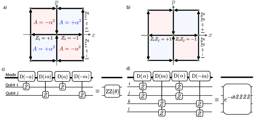
Figure 5: Oscillator-mediated multi-qubit gates. Multi-qubit gates can be implemented in the proposed architecture via a sequence of conditional displacements gates on an oscillator, such that the total enclosed area $A$ corresponds to a geometric phase $e^{2iA}$ imparted on the oscillator. a) Phase-space trajectories arising from the sequence of conditional displacements in Eq. (47), enclosing an area $A=\pm\alpha^{2}Z_{i}Z_{j}$ and enacting the gate $\textrm{ZZ}_{i,j}=\textrm{exp}(-i\frac{\theta}{2}\hat{Z}_{i}\hat{Z}_{j})$ where $\alpha=\sqrt{\theta}/2$. The green circle indicates the starting point. Crucially, the implementation of the gate does not depend upon or alter the initial state of the mode, as all points in phase-space undergo translations of the trajectory shown. b) The circuit diagram corresponding to panel a. Importantly, the implementation of the gate does not depend on or alter the initial state of the modes. c) Phase-space trajectories that implement the four-qubit gate $\textrm{Z}_{\square}$ via the sequence in Eq. (50). In contrast to panel a, all displacements are conditioned on pairs of qubits by leveraging the primitives discussed in Sec. II.2. d) Circuit diagram to realize $e^{-i\frac{\theta}{2}\hat{Z}_{i}\hat{Z}_{j}\hat{Z}_{k}\hat{Z}_{l}}$ requiring four doubly-conditional displacements in sequence.

Specifically, as a particular instance of Eq. (34), we define the operator generated by $\hat{O}_{j}$ and conditioned on the $k$th superparity of mode $i$,

$$\begin{split}\operatorname{CU}_{i,j}^{\bar{\Pi}_{k}}(\theta)&=e^{-i\theta\hat{Z}_{\textrm{anc}}\bar{\Pi}_{ki}\hat{O}_{j}}\\ &=\textrm{SQR}_{\textrm{anc},i}(\vec{\pi}_{k},\vec{0})e^{-i\theta\hat{Z}_{\textrm{anc}}\hat{O}_{j}}\textrm{SQR}_{\textrm{anc},i}(-\vec{\pi}_{k},\vec{0}),\end{split}$$ (40)

where we have made the variable angle $\theta$ explicit for reasons that will become clear shortly. Similarly, we define $\operatorname{CU}_{i,j}^{\hat{\Pi}_{k}}(\theta)$ in analogy to Eq. (38), see Fig. 4b. Here, $\hat{\Pi}_{k}$ is projection operator that returns the $k$th bit of $\hat{n}_{i}$ (and $\bar{\Pi}_{k}$ its corresponding reflection operator, returning $\pm 1$), and $\vec{\pi}_{k}=\{\theta_{0},\theta_{1},\theta_{2},\ldots\}$ with

$$\theta_{n}=\begin{cases}\pi&\text{if $\lfloor n/2^{k}\rfloor$ mod 2 = 1}\\ 0&\text{otherwise}.\end{cases}$$ (41)

For example $\vec{\pi}_{0}=\{0,\pi,0,\pi,\ldots\}$ is equivalent to the parity vector defined below Eq. (28), converting the SQR gate into a qubit rotation controlled on the least-significant (zeroth) bit of $\hat{n}_{i}$. We note that $\bar{\Pi}_{0}\equiv\bar{\Pi}$, where the latter is defined in Eq. (27). Likewise, the choice $\vec{\pi}_{1}=\{0,0,\pi,\pi,\ldots\}$ corresponds to qubit rotation controlled on the first bit of $\hat{n}_{i}$. In general,

$$\textrm{SQR}_{\textrm{anc},i}(\vec{\pi}_{k},\vec{0})=e^{-i\frac{\pi}{2}\hat{X}_{\textrm{anc}}\hat{\Pi}_{ki}},$$ (42)

and the choice $\vec{\pi}_{k}$ enables a qubit rotation controlled on the $k$th bit of $\hat{n}_{i}$.

Applying successive operations controlled on each bit of $\hat{n}_{i}$ in sequence then yields the general form

$$\begin{split}\operatorname{CU}_{i,j}^{f(\hat{\Pi}_{0},\hat{\Pi}_{1},\hat{\Pi}_{2},\ldots)}&=\prod_{k=0}^{K-1}\operatorname{CU}_{i,j}^{\hat{\Pi}_{k}}(\theta_{k})\\ &=\exp\left(-iZ_{\textrm{anc}}\sum_{k=0}^{K-1}\theta_{k}\hat{\Pi}_{ki}\hat{O}_{j}\right),\end{split}$$ (43)

requiring $K=\lceil\log_{2}(n_{\mathrm{max}}+1)\rceil$ iterations of (super)-parity controlled gates, and where $f(\hat{\Pi}_{0},\hat{\Pi}_{1},\hat{\Pi}_{2},\dots)$ is any linear function in the bit operators $\hat{\Pi}_{k}$. Returning to the initial goal of synthesizing $\operatorname{CU}_{i,j}^{\hat{n}}$ in Eq. (39), we note that

$$\hat{n}_{i}=\sum_{k=0}^{K-1}2^{k}\hat{\Pi}_{ki}.$$ (44)

Consequently, choosing $\theta_{k}=2^{k}$ realizes the desired gate. This sequence is shown in Fig. 4c.

As a particular example of this gate that will prove useful in Sec. III.1.4 for implementing density-denstiy interactions, one can choose $\hat{O}_{j}\to\theta\hat{n}_{j}$ to realize the phase-space rotation of one mode controlled on the density of second,

$$\operatorname{RR}_{i,j}(\theta)=e^{-i\theta\hat{Z}_{\textrm{anc}}\hat{n}_{i}\hat{n}_{j}}.$$ (45)

Finally, we emphasize that while our focus has been on synthesizing the density-controlled operator $\operatorname{CU}_{i,j}^{\hat{n}}$, the general form $\operatorname{CU}_{i,j}^{f(\hat{\Pi}_{0},\hat{\Pi}_{1},\hat{\Pi}_{2},\ldots)}$ enables further possibilities beyond this particular choice. Specifically, it allows for operations conditioned on any function $f(\hat{\Pi}_{0},\hat{\Pi}_{1},\hat{\Pi}_{2},\ldots)$ that is linear in the bit operators $\hat{\Pi}_{ki}$. Morevover, we note that an arbitrary function $f(\hat{n}_{i})$ can be realized by iterating the primitive $\operatorname{CU}^{\hat{P}}_{ij}$ a number of times linear in $n_{\textrm{max}}$. This possibility is discussed in our companion work, Ref. [45].

II.6 Oscillator-mediated multi-qubit gates

As the architecture illustrated in Fig. 2 does not include direct couplings between transmons, their utility for encoding fermionic and gauge field degrees of freedom relies on the ability to synthesize transmon-transmon entangling gates using native gates. Here, we adopt an oscillator-mediated approach proposed in our companion work Ref. [45] to realize such entangling gates that bear close similarity to Mølmer-Sørensen gates in trapped-ion platforms [104, 105], and also some parallels to mediated gates in silicon [106, 107, 108]. Crucially, this approach allows for the exact analytical compilation of multi-qubit gates, independent of (and without altering) the initial state of the mediating oscillators in the absence of noise. The core idea is to use a sequence of conditional oscillator displacements that form a closed phase-space path that depends upon the state of the qubits (see, for example, Fig. 5a). Upon completion, this closed path leaves the oscillator unchanged yet imparts a geometric phase on the system that depends upon the state of the qubits, thus enacting the target gate.

To realize these oscillator-mediated multi-qubit gates, we require the ability to enact displacements of the $j$th oscillator conditioned on the $i$th transmon,

$$\mathrm{CD}_{i,j}(\alpha)=e^{\hat{Z}_{i}(\alpha\hat{a}_{j}^{\dagger}-\alpha^{*}\hat{a}_{j})}.$$ (46)

For $i=j$, such conditional displacements can be realized either natively [89] or compiled using conditional-parity gates and unconditional displacements, as shown in Eq. (18); furthermore, as discussed in Ref. [45] and summarized in Sec. II.1, it is possible to synthesize conditional displacements for arbitrary $i$ and $j$ by additionally leveraging a beamsplitter network that links the two sites.

As a particular example, the two-qubit entangling gate $\operatorname{ZZ}_{i,j}(\theta)=\textrm{exp}(-i\frac{\theta}{2}\hat{Z}_{i}\hat{Z}_{j})$ can be realized via a sequence of four conditional displacements,

$$\begin{split}\operatorname{ZZ}_{i,j}(\theta)&=\textrm{CD}_{i,j}(-i\alpha)\textrm{CD}_{i,i}(\alpha)\\ &\times\textrm{CD}_{i,j}(+i\alpha)\textrm{CD}_{i,i}(-\alpha).\end{split}$$ (47)

The corresponding phase-space trajectories and circuit diagram are shown in Fig. 5a and Fig. 5b, respectively. As explained in Ref. [45], this sequence can be further optimized by leveraging conditional displacements on both modes $i$ and $j$ such that each accumulates a geometric phase in parallel, leading to a reduction in gate duration by a factor of $\sqrt{\alpha}$ compared to the above single-mode approach, while also reducing the potential impact of non-idealities such as self-Kerr interactions (anharmonicities). See Ref. [45] for more details.

This strategy can be extended to realize oscillator-mediated $N$-qubit gates that are useful for studying lattice gauge theories. For example, as will be discussed in Sec. IV.1.2, the four qubit gate

$$e^{-i\frac{\theta}{2}\hat{Z}_{i}\hat{Z}_{j}\hat{Z}_{k}\hat{Z}_{l}}$$ (48)

is useful for implementing a magnetic field term in the $\mathds{Z}_{2}$ LGT introduced in Eq. (1). To realize this gate, we modify the sequence in Eq. (47) such that each displacement is conditioned on the joint state of pairs of qubits, e.g., $\hat{Z}_{i}\hat{Z}_{j}$ or $\hat{Z}_{k}\hat{Z}_{l}$, as shown in Fig. 5c. To that end, we define the doubly-conditional displacement as

$$\textrm{CD}^{ZZ}_{i,j,r}(\alpha)=e^{\hat{Z}_{i}\hat{Z}_{j}(\alpha\hat{a}^{\dagger}_{r}-\alpha^{*}\hat{a}_{r})}.$$ (49)

This gate be implemented via the technique described in Sec. II.2. As illustrated in Fig. 5d, the four-qubit term can be exactly realized by sequencing four such doubly-conditional displacements:

$$e^{-i\frac{\theta}{2}\hat{Z}_{i}\hat{Z}_{j}\hat{Z}_{k}\hat{Z}_{l}} =\textrm{CCD}_{i,j,r}(-i\alpha)\textrm{CCD}_{k,l,r}(\alpha)$$

$$\times\textrm{CCD}_{i,j,r}(+i\alpha)\textrm{CCD}_{k,l,r}(-\alpha),$$ (50)

with $\alpha=\sqrt{\theta}/2$.

Similar to the implementation of $\operatorname{ZZ}_{i,j}(\theta)$, it is beneficial to use multiple modes in parallel to accumulate the necessary geometric phase and reduce the displacement parameter $\alpha$. Moreover, this strategy can be extended to realize arbitrary operations of the form $e^{-i\theta\hat{W}}$, where here $\hat{W}$ is an arbitrary-weight Pauli operator. See Ref. [45] for a more complete discussion.

Finally, we note that a similar strategy for oscillator-mediated $N$-body entangling gates has been proposed [109] and demonstrated [110] in trapped-ion platforms. There, spin-dependent squeezing operations are used in place of conditional displacement operators, but the overall framework bears similarity to the strategy described here for the superconducting architecture described in Fig. 2.

II.7 Approximate synthesis of multi-mode gates

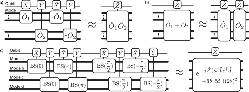
Figure 6: Arbitrary higher-order operator compilation. a) Operator multiplication using the Baker-Campbell-Hausdorff formula. b) Operator addition using the Trotter formula. c) Example: compilation of qubit-conditional quartic term. Note that these methods are only exact if $[\hat{O}_{1},\hat{O}_{2}]=0$. The variable parameter $\theta$ is omitted from the beamsplitters $\operatorname{BS}$ for ease of notation as it is the same parameter which enters all of them. Ancilla-conditional operations can be synthesized using the method described in Sec. II.2.

To approximately implement arbitrary multi-mode operations that fall outside of the form in Sec. II.3 and Sec. II.5, we use the method introduced in Ref. [102]. It relies on a variant of the Baker-Campbell-Hausdorff (BCH) formula,

$$e^{\hat{A}t}e^{\hat{B}t}e^{-\hat{A}t}e^{-\hat{B}t}=e^{[\hat{A},\hat{B}]t^{2}+O\left(t^{3}\right)}.$$ (51)

The key insight is to choose the operators $\hat{A}$, $\hat{B}$ such that they enact commuting bosonic operations $\hat{O}_{1}$, $\hat{O}_{2}$ (possibly acting on distinct sets of different modes), but conditioned on the same qubit with respect to non-commuting Pauli operators, e.g., using the method described in Sec. II.2. For example, we can leverage this idea as follows:

$$\Gamma_{1,2} =e^{i\hat{X}\hat{O}_{1}t}e^{i\hat{Y}\hat{O}_{2}t}e^{-i\hat{X}\hat{O}_{1}t}e^{-i\hat{Y}\hat{O}_{2}t}$$

$$=e^{[\hat{X}\hat{O}_{1},\hat{Y}\hat{O}_{2}](-it)^{2}+O\left(t^{3}\right)},$$

$$=e^{-2i\hat{Z}\hat{O}_{1}\hat{O}_{2}t^{2}+O\left(t^{3}\right)}.$$ (52)

See also Fig. 6a for the circuit diagram. In this way, one can implement operator multiplication between $O_{1}$ and $O_{2}$. Combining this with the Trotter formula to implement addition, following Ref. [102] and Fig. 6b, we can implement exponentials of non-linear functions in the creation and annihilation operators.

When the commutator obtained through the above BCH formula contains both desired and undesired high-order mode terms, we can cancel the latter by applying Eq. (52) a second time with a different choice of operators. Via the Trotter formula we then obtain:

$$\Delta_{1,2} =e^{-2i\hat{Z}\hat{O}_{1}\hat{O}_{2}t^{2}}e^{-2i\hat{Z}\hat{O^{\prime}_{1}}\hat{O}^{\prime}_{2}t^{2}}+O\left(t^{3}\right)$$

$$=e^{-2i\hat{Z}\left(\hat{O}_{1}\hat{O}_{2}+\hat{O}^{\prime}_{1}\hat{O}^{\prime}_{2}\right)t^{2}}+O\left(t^{3}\right),$$ (53)

where the error term will be different between the two lines and we rewrote the error as an additive error by Taylor expanding the exponential. Here, each term is conditioned on the same qubit, either natively or via SWAP operations between the qubits or the modes.

In Fig. 6c, we use this technique to approximately synthesize the four mode operator,

$$e^{-i\hat{Z}\left(\hat{a}^{\dagger}\hat{b}\hat{c}^{\dagger}\hat{d}+\mathrm{h.c.}\right)(2\theta)^{2}}.$$ (54)

which will later be used in Sec. IV.2.2 to realize the plaquette term in the $U(1)$ quantum link model.

II.8 Dual-rail qubits

While so far we have discussed primitives for mapping the model to the hardware with transmons being used as data or ancillary qubits and the modes being used to encode bosonic degrees of freedom, another possibility is to use the modes to encode qubits. In this section, we discuss such an encoding: the dual-rail qubit. The core idea is to encode a single qubit using a pair of cavity modes that share a single photon. The location of the photon then represents the qubit state [98, 91, 101]

$$|0\rangle_{\mathrm{DR}} =|0,1\rangle$$ (55)

$$|1\rangle_{\mathrm{DR}} =|1,0\rangle.$$ (56)

Denoting the cavity photon numbers to be $|n^{a},n^{b}\rangle$, we see that the Pauli $Z$ operator has various equivalent representations,

$$\hat{Z}^{\mathrm{DR}} =\hat{n}^{b}-\hat{n}^{a}$$ (57)

$$=\mathds{1}-2\hat{n}^{a}=2\hat{n}^{b}-\mathds{1}$$ (58)

$$=e^{i\pi\hat{n}^{a}}=-e^{i\pi\hat{n}^{b}},$$ (59)

where we have used the fact that $\hat{n}^{a}+\hat{n}^{b}=\mathds{1}$. The remaining Pauli operators are given by,

$$X =a^{\dagger}b+ab^{\dagger}$$ (60)

$$Y =i[a^{\dagger}b-ab^{\dagger}].$$ (61)

Note that this is simply the Schwinger boson representation of a spin one-half.

The primary advantage of the dual-rail encoding is that photon loss in either the left or right cavity results in an erasure error that is detectable via joint-parity measurements [98, 91, 101]. Furthermore, single-qubit operations are straightforward: rotations about any axis in the azimuthal plane can be carried out with a beamsplitter, and rotations about the $Z$ axis correspond to a phase-space rotation of one of the modes (up to a global phase). Furthermore, it has been shown that one can construct a universal gate set that enables detection of ancillary transmon dephasing and relaxation errors, the latter made possible by leveraging three levels of the transmon qubit [100]. Consequently, for models that require many qubit-qubit gates (such 2D fermionic problems that necessitate fermionic SWAP networks), the dual-rail encoding is potentially advantageous for mitigating errors with post-selection in near-term experiments.

ZZ${}_{i,j}^{\mathrm{DR}}(\theta)$. As an example of an entangling gate between dual-rail qubits, we consider the compilation of $\operatorname{ZZ}^{\mathrm{DR}}_{i,j}(\theta)=e^{-i(\theta/2)\hat{Z}^{\mathrm{DR}}_{i}\hat{Z}^{\mathrm{DR}}_{j}}$. Using the fact that $\hat{Z}^{\mathrm{DR}}_{i}=\mathds{1}-2\hat{n}_{i}^{a}$, this gate can be expressed as

$$\begin{split}\operatorname{ZZ}_{i,j}^{\mathrm{DR}}(\theta)&=e^{-i\frac{\theta}{2}}e^{-i2\theta\hat{n}_{i}^{a}\hat{n}_{j}^{a}}e^{i\theta\hat{n}_{i}^{a}}e^{i\theta\hat{n}_{j}^{a}}\\ =&e^{-i\frac{\theta}{2}}(\bra{0}_{\rm anc}\otimes\openone)\operatorname{RR}_{i,j}(2\theta)(\ket{0}_{\rm anc}\otimes\openone)\\ &\times\operatorname{R}_{i}(-\theta)\operatorname{R}_{j}(-\theta),\end{split}$$ (62)

where, for simplicity of notation, we have dropped the superscript $a$. Therefore, this gate can be realized by combining a pair of phase-space rotations with the technique introduced in Sec. II.5 to realize $\operatorname{RR}(2\theta)$ – see Eq. (45).

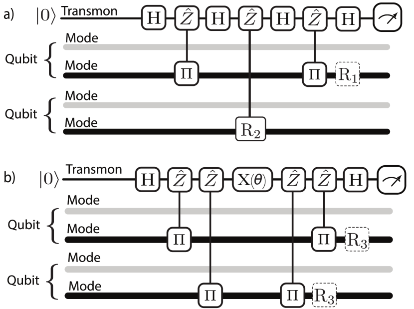
Figure 7: Dual rail entangling gate. Both panels show compilation methods for $\textrm{ZZ}(\theta)=\textrm{exp}(-i\frac{\theta}{2}\hat{Z}_{i}\hat{Z}_{j})$. The gray and black colors of the mode wires correspond to the location of the boson when the dual-rail qubit is in state $\ket{0}$ or $\ket{1}$, respectively. In both methods, the ancilla transmon must start out in $\ket{0}$. a) Circuit as compiled using the methods shown in Sec. II.3. $\operatorname{R}_{1}=R(\pi-\theta),\>\operatorname{R}_{2}=R(-2\theta)$. The measurement is optional - it can help detect amplitude dampling errors. b) Method presented in  [100] for implementing $\operatorname{ZZ}(\theta)$. $\operatorname{R}_{3}=\operatorname{R}(\pi)$. The $\operatorname{Z}$-conditional rotation gates refer to $\operatorname{CR}(\theta)$. The measurement will help detect amplitude dampling errors as well as phase errors [100].

However, note that in the dual rail encoding, the boson number of mode $i$ is restricted to either 0 or 1, which means that the SQR gate used to implement Eq. (45) of Sec. II.5 can be reduced to a conditional phase-space rotation up to single qubit operations. For the choice of $\vec{\theta}=\vec{\pi}_{0}$, this conditional rotation in the $\{\ket{0},\ket{1}\}$ subspace corresponds to a conditional-parity gate:

$$\operatorname{SQR}_{i,j}(\vec{\pi}_{0},\vec{0})\Rightarrow\operatorname{H}_{i}\operatorname{C\Pi}_{i,j}\operatorname{H}_{i}=\operatorname{C\Pi}^{X}_{i,j}$$ (63)

where $\operatorname{H}_{i}$ is a Hadamard gate on qubit $i$, and we have defined the shorthand $\operatorname{C\Pi}^{X}_{i,j}$ to denote the $X$-conditional parity gate. Therefore, we can re-write the decomposition of $\operatorname{ZZ}^{\rm DR}_{i,j}(\theta)$ as:

$$\begin{split}\operatorname{ZZ}_{i,j}^{\mathrm{DR}}(\theta)=&e^{-i\frac{\theta}{2}}(\bra{0}_{\rm anc}\otimes\openone)\operatorname{C\Pi}^{X}_{\textrm{anc},i}\operatorname{CR}_{\textrm{anc},j}(-2\theta)\operatorname{C\Pi}^{X}_{\textrm{anc},i}\\ &\times(\ket{0}_{\rm anc}\otimes\openone)\operatorname{R}_{i}(\pi)\operatorname{R}_{j}(\theta)\operatorname{R}_{i}(-\theta)\operatorname{R}_{j}(-\theta),\end{split}$$ (64)

where the top line, up to the global phase, corresponds to $\operatorname{RR}(2\theta)$ in the truncated dual rail subspace. The complete circuit (with single qubit rotations simplified) is presented in Fig. 7a. We note that sequential ancilla-conditional gates using the same transmon (but distinct modes) requires implicit SWAP operations not shown.

While exact, the circuit in Fig. 7a does not enable the detection of transmon dephasing errors. To that end, a scheme to synthesize error-detectable entangling gates was presented in Ref. [100]. It leverages an “exponentiation circuit” that interleaves ancilla-controlled unitaries (controlled-$\hat{P}$) with ancilla rotations to construct any unitary $\widehat{P}(\theta)=\exp\left(-i\frac{\theta}{2}\hat{P}\right)$, provided $\widehat{P}^{2}=\hat{\mathds{1}}$. Returning to the case of $\operatorname{ZZ}_{i,j}^{\mathrm{DR}}(\theta)$, this gate can be constructed following this prescription in the previous paragraph, choosing $\widehat{P}=\hat{Z}\otimes\hat{Z}$ and implementing controlled-$\hat{P}$ using a pair of conditional-parity gates. We illustrate the full implementation in terms of our discrete gate set in Fig. 7b. Notably, this latter circuit can be understood as a further decomposition of its counterpart in Fig. 7a, where the middle $\operatorname{CR}(-2\theta)$ gate is broken into conditional-parity gates and single qubit operations using the identities in Sec. II.3.

While both circuits are mathematically equivalent, the structure of Fig. 7b enables partial error detection of some of the dominant errors, including transmon dephasing. However, it comes at the cost of requiring four conditional-parity gates, each with a duration $T_{\textrm{C}\Pi}=\pi/\chi$. Thus, ignoring the cost of SWAPs and single-qubit and mode operations, the minimum duration of $\operatorname{ZZ}_{i,j}^{\mathrm{DR}}(\theta)$ using the method in Fig. 7b is $T_{b,\textrm{min}}=4\pi/\chi$, independent of $\theta$. In contrast, the method in Fig. 7a requires $T_{a,\textrm{min}}=2(\pi+\theta)/\chi$, a reduction for even the maximal entangling case $\theta=\pi/2$. Thus, there is a tradeoff in error detectability and gate duration, and the approach in Fig. 7a may therefore be beneficial in certain contexts, particularly for repeated applications of $\operatorname{ZZ}_{i,j}^{\mathrm{DR}}(\theta)$ for small $\theta$ (e.g., for Trotterized circuits).

III Implementation of matter fields

In this section, we leverage the compilation strategies of the previous section to realize the unitary time evolution operator $e^{-i\hat{H}t}$ for a range of common Hamiltonian terms involving bosonic and fermionic matter. For the purely bosonic matter terms, in Sec. III.1, we show that some of the common dynamics terms correspond to native gates, and others to terms that can be realized using the compilation techniques in the previous section. For the purely fermionic matter terms, in Sec. III.2, we demonstrate how to encode fermionic SWAP networks into various qubit encodings possible in hybrid oscillator-qubit hardware. For the fermion-boson interaction terms, in Sec. III.3, we present novel compilation strategies specific to hybrid oscillator-qubit hardware. We summarize these results in Tab. 3 and Tab. 4. All terms involving gauge fields will be treated in Sec. IV.

III.1 Bosonic matter

$\hat{H}$	$e^{-i\hat{H}t}$ Gates	Details
$\sum_{\braket{i,j}}J_{i,j}\left(e^{i\varphi}\hat{a}^{\dagger}_{i}\hat{a}_{j}+\mathrm{h.c.}\right)$	$\textrm{BS}_{i,j}(\varphi,\theta)$	Tab. 1, Sec. III.1.1
$\sum_{i}\mu_{i}\>\hat{n}_{i}$	$\operatorname{R}_{i}(\theta)$	Tab. 1, Sec. III.1.2
$\sum_{i}U_{i}\hat{n}_{i}^{2}$	$\mathrm{SNAP}_{i}(\vec{\theta})$	Tab. 1, Sec. III.1.3
$\sum_{\braket{i,j}}V_{i,j}\hat{n}_{i}\hat{n}_{j}$	$\operatorname{RR}_{i,j}(\theta)$	Fig. 4, Sec. III.1.4

Table 3: Bosonic Hamiltonian terms and the implementation of $e^{-i\hat{H}t}$ in the proposed architecture. Note that for the onsite interaction, an ancillary qubit is required – see App. B for an ancilla-free implemention that leverages the Gauss’ss law constraint in a $\mathbb{Z}_{2}$ lattice gauge theory.

In this section, we discuss the most common Hamiltonian terms for bosonic matter fields (which typically involve small powers of the creation and annihilation operator). The results are summarized in Table 3. We first discuss hopping as this is the most elementary term coupling bosonic modes. We then discuss terms related to powers and products of number operators $\hat{n}$: the onsite potential (linear in $\hat{n}$), the onsite interaction (quadratic in $\hat{n}$), and the intersite interaction (bilinear, $\hat{n}_{i}\hat{n}_{j}$). We map the bosonic matter fields to the native bosonic modes supported in the hybrid oscillator-qubit hardware in Fig. 2.

III.1.1 Hopping

The time evolution operator $e^{-i\hat{H}t}$ for the hopping interaction $\hat{H}=\sum_{\braket{i,j}}J_{i,j}\left(\hat{a}^{\dagger}_{i}\hat{a}_{j}+\mathrm{h.c.}\right)$ between bosonic matter sites can be implemented via Trotterization using a sequence of beamsplitter gates $\operatorname{BS}_{i,j}(\varphi,\theta)$ (defined in Tab. 1) by choosing $\theta=Jt$. Furthermore, a static gauge field (vector potential) appears as a complex phase in the hopping $J\rightarrow Je^{i\varphi}$ [111], and is important to simulate models of the fractional quantum Hall effect [112]. To implement this term, one can simply adjust the phase $\varphi$ of the beamsplitter on each link such that a net phase is accumulated in moving around each plaquette.

III.1.2 Onsite potential

The onsite potential is $\hat{H}=\sum_{i}\mu_{i}\hat{n}_{i}$, with $\hat{n}_{i}=\hat{a}_{i}^{\dagger}\hat{a}_{i}$ $\mu_{i}\in\mathbb{R}$. The time evolution of this term can be implemented on each site separately using a phase space rotation gate (defined in Tab. 1) as is shown in Tab. 3.

As mentioned previously in Sec. I.2, it is possible to absorb phase space rotations into operators that include creation/annihilation operators such as beamsplitters. In particular, a constant site energy shift can be created with a fixed frequency detuning of the microwave tones that activate the beamsplitters.

III.1.3 Onsite interaction

The bosonic onsite interaction is $\sum_{i}U_{i}\hat{n}_{i}^{2}$ with $U_{i}\in\mathbb{R}$. To implement the time evolution operator for this term, one can use the Selective Number-dependent Arbitrary Phase (SNAP) gate [90]. $\mathrm{SNAP}_{i}(\vec{\theta})$, as defined in Tab. 1, operates in the strong-dispersive coupling regime where the qubit frequencies depend on the mode occupation such that the SNAP gate effectively imparts an independently chosen phase to the system comprising qubit and mode, for each vaue of the mode occupation. Choosing $\theta_{k}=U_{i}k^{2}t$, where $k$ is photon number corresponding to a particular Fock state implements the onsite interaction $\hat{n}^{2}_{i}$ on the $i$th mode. This procedure additionally requires an ancillary qubit initialized to the state $\ket{0}$.

III.1.4 Intersite interaction

The time-evolution of a nearest-neighbor density-density interaction $\hat{H}=\sum_{\braket{i,j}}J_{i,j}\hat{n}_{i}\hat{n}_{j}$ between two modes in separate cavities, which is useful for example in simulation of the extended Hubbard model or dipolar interacting systems, can be implemented with the method proposed in Sec. II.5 via the $\operatorname{RR}(\theta)$ gate defined in Eq. (45):

$$e^{-iJ_{i,j}\hat{n}_{i}\hat{n}_{j}t}= (\bra{0}_{\rm anc}\otimes\openone)\operatorname{RR}_{i,j}(J_{i,j}t)(\ket{0}_{\rm anc}\otimes\openone).$$ (65)

Here, we have used an ancillary qubit that begins and (deterministically) ends in the state $\ket{0}_{\rm anc}$. As discussed in Sec. II.5 and shown in Table 2, this gate requires a native gate count that is logarithmic in the bosonic cutoff $n_{\mathrm{max}}$. Long-range interactions between sites $i$ and $j$ can be implemented at the cost of bosonic SWAP gate count that is linear in the Manhattan-metric distance between the sites.

III.2 Fermionic matter

In this section, we show that it is possible to treat purely fermionic terms within our proposed hybrid qubit-oscillator architecture. While this is not an area in which to expect an explicit advantage over qubit-only hardware, we show that no significant cost is added compared to existing qubit platforms.

We treat fermionic matter by mapping the fermions to qubits and rely on FSWAP networks [113] of Jordan-Wigner (JW) strings for a low-depth implementation. For an overview of the set of operations required to implement $e^{-i\hat{H}t}$ for a $2$D fermionic Hamiltonian $\hat{H}$ in qubit-based hardware, see App. A. In summary, the two-dimensional lattice is virtually mapped to a one-dimensional chain. Nearest-neighbour hoppings in the $2$D lattice become either nearest-neighbour hoppings in the $1$D JW chain (which we call “JW-adjacent”) or long-range hoppings (which we call “non-JW-adjacent”). The former hoppings only require iSWAP operations, whereas the latter also require FSWAP operations. Gates that involve the fermionic number density are mapped to gates involving the $\hat{Z}$ operator and do not add any overhead associated with the Jordan-Wigner encoding.

We first summarize the possibilities for encoding fermions (i.e., implementing iSWAP and FSWAP operations) either in transmons (Sec. III.2.1) or in cavity dual-rail qubits (Sec. III.2.2). While the former is more hardware efficient, the latter enables error-detection and, as a result, is a particularly promising avenue for near-term simulations on noisy hardware. The high-level results for both encodings are summarized in Table 4. In Sec. III.2.3, we discuss the fidelity of gates that underly the simulation of fermions in the dual-rail encoding.

$\hat{H}$	Intermediary Step	Implementation	$e^{-i\hat{H}t}$ Gates	Details
$\sum\limits_{\braket{i,j}}J_{i,j}\left(\hat{c}^{\dagger}_{i}\hat{c}_{j}+\mathrm{h.c.}\right)$	$(1)\>\mathrm{FSWAP}$ $(2)\>\mathrm{iSWAP}(\lambda)$	Dual Rail	$(1)\>\operatorname{SWAP}_{i,j}$, $\operatorname{C\Pi}_{i,j}$, $\operatorname{R^{\varphi}}_{i}(\theta)$, $\operatorname{R}_{i}(\theta)$ $(2)\>\operatorname{BS}_{i,j}(\varphi,\theta)$, $\operatorname{C\Pi}_{i,j}$, $\operatorname{R^{\varphi}}_{i}(\theta)$	Fig. 8, Sec. A.1
		Transmon	$(1)\>\operatorname{SWAP}_{i,j},\operatorname{CD}_{i,j}(\theta),\operatorname{R}^{Z}_{i}(\theta)$ $(2)\>\operatorname{CD}_{i,j}(\theta)$, $\operatorname{R^{\varphi}_{i}(\theta)}$	Fig. 5, Sec. II.6
$\sum_{i}\mu_{i}\hat{n}_{i}$	$\exp\left(-i\lambda\hat{Z}_{i}\right)$	Dual Rail	$\operatorname{R}_{i}(\theta)$	Tab. 1, Sec. A.3
		Transmon	$\operatorname{R}^{z}_{i}(\theta)$	Tab. 1
$\sum_{\braket{i,j}}V_{i,j}\hat{n}_{i}\hat{n}_{j}$	$\exp\left(-i\frac{\lambda}{2}\hat{Z}_{i}\hat{Z}_{j}\right)$	Dual Rail	$\operatorname{C\Pi_{i,j}}$, $\operatorname{R^{\varphi}_{i}(\theta)}$	Sec. A.3
		Transmon	$\operatorname{CD}_{i,j}(\theta),\operatorname{C\Pi}_{i,j}$	Fig. 5, Sec. II.6

Table 4: Fermionic Hamiltonian Terms. We list native gates required for the implementation of essential Hamiltonian terms in the proposed architecture. $\lambda$ is proportional to time and the Hamiltonian parameter. The fourth column only lists the necessary gates, but does not provide the complete circuits – these are described in the relevant sections to which there are pointers in the last column of the table. The onsite term $\sum_{i}U_{i}\hat{n}_{i,\gamma}\hat{n}_{i,\delta}$ contains terms which depend on $\gamma$ and $\delta$ which refer to the fermion spin. Mapping these two spin species to two different fermionic sites $i$ and $j$ casts this term into the same form as the nearest neighbor term in the bottom row of the table.

III.2.1 Transmon qubits

In the proposed 3D post-cavity circuit QED setup, encoding the fermion into the transmon enables the use of the cavities for a separate purpose, such as for representing the phonon modes in the Hubbard-Holstein model, or for encoding bosonic gauge fields as will be demonstrated in the context of a $\mathbb{Z}_{2}$ lattice gauge theory later in this work.

As the architecture illustrated in Fig. 2 does not include direct couplings between transmons, we rely on the oscillator-mediated compilation strategy discussed in Sec. II.6 to realize entangling gates, $\operatorname{ZZ}_{i,j}(\theta)$ in particular. We reemphasize that this approach does not require that the mediating oscillators are in a known, particular state. Thus, they can simultaneously be used to encode matter or gauge degrees of freedom.

III.2.2 Dual-rail qubits 

We now discuss the separate possibility to map fermions to dual rail qubits. As discussed in Sec. II.8, dual rail qubits present a number of advantages, including the possibility for detection of photon loss and ancilla relaxation and dephasing errors [100].

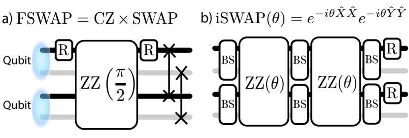
Figure 8: Fermionic SWAP network operations in dual rail qubits. a) FSWAP gate. b) Arbitrary-angle iSWAP gate for implementing the hopping on Jordan-Wigner adjacent sites. The vertical lines connecting the crosses are $\operatorname{SWAP}$ gates between the bosonic modes (with the pair together realizing a $\operatorname{SWAP}$ gate between dual rail qubits), $\operatorname{R}$ is shorthand for a phase space rotation gate $\operatorname{R}(\frac{\pi}{4})$, $\operatorname{BS}$ denotes a beamsplitter $\operatorname{BS}(\varphi,\tilde{\theta})$ defined in Tab. 1 and the $\operatorname{ZZ}(\theta)$ gate acting on the dual rail qubits is defined in section II.8. The gray and black colors of the mode wires correspond to the location of the boson when the dual-rail qubit is in state $\ket{0}$ or $\ket{1}$, respectively.

FSWAP. For the non-JW-adjacent hopping terms, a full $\operatorname{SWAP}_{i,j}$ operation is required between the dual-rail qubits as part of the FSWAP operation. This can be implemented by separately applying a $\operatorname{SWAP}_{i,j}$ operation between the cavities representing the $\ket{1}$ and $\ket{0}$ states, as represented in Fig. 8. As described in App. A.1, the FSWAP also requires a $\operatorname{CZ}_{i,j}(\theta)$ gate which is equivalent to the $\operatorname{ZZ}_{i,j}(\theta)$ gate up to single qubit phase gates. As discussed in Sec. II.8 (c.f. App. A.1), these single qubit phase gates correspond to phase-space rotations on the mode which hosts the boson when the dual rail qubit is in the state $\ket{1}$. The corresponding circuit is shown in Fig. 8a.

iSWAP($\theta$). For the JW-adjacent hopping terms, following Eq. (182), we only need to implement a variable-angle iSWAP gate defined in Fig. 8b. This requires only $\operatorname{ZZ}_{i,j}(\theta)$ gates and $\operatorname{H}$ and $\operatorname{S}$ single-qubit rotations. An error-detectable implementation of $\operatorname{ZZ}_{i,j}(\theta)$ between dual-rail qubits was presented in Ref. [100] and is summarized here in Sec. II.8. We show the circuit for implementing $e^{\-i\theta\left(\hat{X}_{i}\hat{X}_{i+1}+\hat{Y}_{i}\hat{Y}_{i+1}\right)}$ at the level of the modes supporting the dual-rail qubits in Fig. 8b.

III.2.3 Comparing advantages of different platforms for encoding fermions

We note that different platforms have different advantages for implementing non-JW-adjacent hopping.

In a planar transmon qubit array with tunable couplers, FSWAP operations can be implemented using the FSIM gate using FSIM$(\theta=\frac{\pi}{2},\phi=0)$ with high fidelity ($\approx 0.9930$) [114]. $e^{i\theta\left(\hat{X}\hat{X}+\hat{Y}\hat{Y}\right)}$ operations can be implemented using FSIM$(\theta,\phi=0)$, also with high fidelity (currently $\approx 0.9962$) [114].

In the ion trap QCCD architecture [115, 116] FSWAP operations can be implemented using a SWAP operation and a $\operatorname{ZZ}(\pi/2)$. Because the ions can be physically moved around the circuit to achieve all-to-all connectivity, the fidelity of the FSWAP operation reduces to the fidelity of $\operatorname{ZZ}(\pi/2)$ which is currently 0.9980 [116, 115], yielding a fidelity advantage compared to the planar transmon implementation. Furthermore, $e^{i\theta\left(\hat{X}\hat{X}+\hat{Y}\hat{Y}\right)}$ can be implemented with two $\operatorname{ZZ}(\theta)$ which currently has a fidelity of $\approx 0.9960$ [115].

In the circuit QED setup using dual rail qubits, as discussed, we can use the $\operatorname{ZZ}(\theta)$ gates to implement fermionic SWAP networks similar to ion trap QCCD architectures. Beamsplitter operations in the high-Q cavity setup required for a SWAP operation between dual-rail qubits have very high fidelity of $0.9992$ [86, 103] (comparable to single-qubit gates on transmons). Importantly, we can use the error-detection capability to increase the fidelity of the operations with post-selection, as discussed in [100, 98]. This results in $\operatorname{ZZ}(\pi/2)$ gates with a theoretically calculated fidelity in the presence of noise and post-selection of $\approx 0.9999$ [100], for a pure dephasing channel with time $T_{\phi}=200$ $\mu$s. The error detection comes at the price of a post-selection requirement, leading to a shot overhead. For the above value of $T_{\phi}$, it was estimated that an error would be detected in $2\%$ [100] of shots. While this percentage increases exponentially with circuit depth, even for $100$ $\operatorname{ZZ}_{i,i+1}(\theta)$ gates, only $1-(1-0.02)^{100}\approx 87\%$ of shots would have to be discarded due to a detected error. This leads to a shot overhead of a factor of $1/(1-87\%)\approx 7.7$.

III.3 Fermion-boson interactions

Here we compile the unitary time evolution operator for two paradigmatic fermion-boson models: phonon-electron interactions in solids and the coupling of strong light fields with electrons. Employing the techniques of the previous sections, we discuss the use of either transmons or dual rail qubits to encode the fermionic matter, and employ modes to represent the bosonic matter.

III.3.1 Phonon-matter interactions

The Holstein model [117] describes (dispersionless) optical phonons in the solid state coupled to the density of electrons. It consists of a kinetic energy term for the electrons (c.f. first row in Tab. 4), an onsite potential term for for the phonons (c.f. Sec. III.1.2) as well as an electron-phonon interaction term

$$\hat{H}=\sum_{i}g_{i}\hat{c}^{\dagger}_{i}\hat{c}_{i}(\hat{a}_{i}^{\dagger}+\hat{a}_{i}).$$ (66)

To implement the latter, note that in the Jordan-Wigner encoding, independent of the dimension, this Hamiltonian term becomes equivalent to the Spin-Holstein coupling [118],

$$\hat{H}=\sum_{i}\frac{g_{i}}{2}(\hat{Z}_{i}+1)(\hat{a}_{i}^{\dagger}+\hat{a}_{i}).$$ (67)

Time evolution under this Hamiltonian can be easily implemented since all terms in the sum commute and each has a simple implementation; the term proportional to $\hat{Z}_{i}$ generates a conditional displacement gate and the remaining term can be eliminated by a simple coordinate frame shift for each oscillator (resulting in a constant chemical potential shift for the fermions).

Transmon qubits. If the qubits are mapped to transmon qubits, conditional displacements can be compiled using conditional parities $\operatorname{C\Pi}_{i,j}$ (Tab. 1) and a displacement $\operatorname{D}_{i}(g_{i}t/2)$. This control was discussed in Sec. II.2 and is illustrated in Fig. 3a.

Dual-rail qubits. In the case of dual-rail qubits, $\hat{Z}_{i}^{\mathrm{DR}}=e^{i\pi\hat{n}_{i,1}}$, where the subscripts $i,1$ indicates the mode which hosts the boson when the dual rail qubit is in state $\ket{1}$. This means that the required dual rail qubit-conditional displacement will take the form $e^{-i\theta e^{i\pi\hat{n}_{i,1}}(\hat{a}_{j}^{\dagger}+\hat{a}_{j})}$, where $\theta=g_{i}t/2$. This is a displacement conditioned on the parity of another mode $\{i,1\}$ and can be realized by $\operatorname{CU}^{\bar{\Pi}}_{i,j}$, whose compilation is presented in Sec. II.3. The full operation illustrated in Fig. 9 is as follows:

$$e^{-i\theta\hat{Z}_{i}^{\mathrm{DR}}(\hat{a}_{j}^{\dagger}+\hat{a}_{j})}=$$

$$\bra{0}_{\rm anc}\operatorname{C\Pi}^{X}_{\textrm{anc},i}\operatorname{CD}_{\textrm{anc},j}(i\theta)\operatorname{C\Pi}^{X}_{\textrm{anc},i}\operatorname{R}_{i}(\pi)\ket{0}_{\rm anc},$$ (68)

where $\operatorname{CD}(\alpha)$ corresponds to a conditional displacement gate as defined in Table 1, and $\operatorname{C\Pi^{X}}$ denotes the Hadamard-conjugated conditional parity gate introduced in Eq. (63). The subscript ‘anc’ refers to the ancilla transmon qubit which is initialized to $\ket{0}_{\textrm{anc}}$ and guaranteed to end in $\ket{0}_{\textrm{anc}}$ at the end of the sequence unless an error occurred – a fact which could be used for error-detection purposes as previously mentioned.

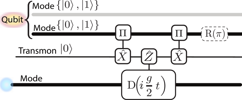
Figure 9: Phonon-matter interactions. A circuit that implements a displacement on a mode conditioned on $\hat{Z}^{\textrm{DR}}$ of a dual rail qubit. This can be used to realize time evolution for a duration $t$ under the Hamiltonian in Eq. (67) (up to an unconditional displacement).

III.3.2 Light-matter interactions

When light interacts with charged matter on a lattice, for instance when a material is placed in an optical cavity, the Hamiltonian is given by [119]

$$\hat{H}=\omega\hat{a}^{\dagger}\hat{a}-J\sum_{\langle i,j\rangle}\hat{c}^{\dagger}_{i}\hat{c}_{j}e^{i\frac{g}{\sqrt{L}}(\hat{a}^{\dagger}+\hat{a})}+\mathrm{h.c.}$$ (69)

for a single light mode $\hat{a}$, where $\omega$ corresponds to the free evolution of the photons, $J$ is the strength of the hopping, $g$ is a coupling constant which depends on the specifics of the system, such as the geometry and material composition of the cavity, and $L$ is the number of lattice sites. Within the Peierls substitution approximation, the exponential term, $\tilde{A}=\frac{g}{\sqrt{L}}(\hat{a}^{\dagger}+\hat{a})$, is given by the particle charge multiplied the line integral of the electromagnetic vector potential along the link from site $j$ to site $i$.

For small $g/\sqrt{L}$ the exponent in the second term can be expanded:

$$\hat{H} =\omega\hat{a}^{\dagger}\hat{a}-\frac{J}{2}\sum_{\langle i,j\rangle}\left(\hat{c}^{\dagger}_{i}\hat{c}_{j}+\mathrm{h.c.}\right)$$

$$+\frac{gJ}{\sqrt{L}}(\hat{a}^{\dagger}+\hat{a})\sum_{\langle i,j\rangle}\hat{c}^{\dagger}_{i}\hat{c}_{j}+O\left(J\frac{g^{2}}{L}\right).$$ (70)

The first term can be implemented using a bosonic phase-space rotation as discussed in Sec. III.1.2. The second term corresponds to fermionic hopping, and can be implemented using the strategy of App. A.1 for fermions encoded in either transmons or dual rail qubits. The second term can be reexpressed as $\exp\left(-it\frac{gJ}{\sqrt{L}}(\hat{a}^{\dagger}+\hat{a})\hat{X}_{i}\hat{X}_{i+1}\right)\exp\left(-it\frac{gJ}{\sqrt{L}}(\hat{a}^{\dagger}+\hat{a})\hat{Y}_{i}\hat{Y}_{i+1}\right)$ for Jordan-Wigner adjacent sites. This corresponds to two doubly-conditional displacements, i.e., conditioned on two qubits, with single qubit rotations.

Transmon qubits. If the qubits are mapped to transmon qubits, doubly-conditional displacements can be compiled using the technique described in Sec. II.2 and illustrated in Fig. 3b. It requires a pair of conditional parity gates $\operatorname{C\Pi}$ (Tab. 1) and a conditional displacement $\operatorname{CD}(\alpha)$ (or alternatively, two pairs of conditional parity gates and an unconditional displacement).

Dual-rail qubits. If the qubits are mapped to dual-rail qubits, doubly-conditional displacements can be synthesized by iterating the compliation strategy for the singly-conditional displacement in Eq. (68), there developed in the context of phonon-matter interactions. The full sequence is as follows:

$$e^{-i\theta\hat{Z}^{\mathrm{DR}}_{i}\hat{Z}^{\mathrm{DR}}_{j}(\hat{a}_{k}^{\dagger}+\hat{a}_{k})}=$$

$$(\bra{0}_{\rm anc}\otimes\openone)\operatorname{C\Pi}^{X}_{{\rm anc},i}\operatorname{C\Pi}^{X}_{{\rm anc},j}\operatorname{CD}_{\textrm{anc},k}(i\theta)$$

$$\times\operatorname{C\Pi}^{X}_{{\rm anc},j}\operatorname{C\Pi}^{X}_{{\rm anc},i}\operatorname{R}_{i}(\pi)\operatorname{R}_{j}(\pi)(\ket{0}_{\rm anc}\otimes\openone),$$ (71)

where, similar to previous gates, we have projected out the ancillary qubit, which is initialized to $\ket{0}_{\textrm{anc}}$ and guaranteed (in the absence of noise) to be disentangled at the end of the sequence. With the above gate realized, single dual rail qubit gates (i.e., beam splitters) can be used to rotate the operator $\hat{Z}^{\rm DR}\hat{Z}^{\rm DR}$ to $\hat{X}^{\rm DR}\hat{X}^{\rm DR}$ or $\hat{Y}^{\rm DR}\hat{Y}^{\rm DR}$, enabling the implementation of all desired gates.

IV Implementation of gauge fields and gauge-matter coupling

In this section, we present implementations of $e^{-i\hat{H}t}$ for pure gauge Hamiltonian terms – i.e., for the electric and magnetic fields – and for the gauge-invariant hopping which couples the gauge fields to matter. In particular, we discuss the implementation of these terms for the two illustrative examples in $(2+1)$D: a $\mathbb{Z}_{2}$ gauge field and a $U(1)$ gauge field, each playing a vital role in the paradigmatic LGTs discussed in Sec. I.1. However, we emphasize that due to the digital nature of our implementations, more complex models can implemented beyond those in Sec. I.1 using techniques in this section, for instance models that contain both $\mathbb{Z}_{2}$ and $U(1)$ fields coupled to the same matter fields.

We present the implementation of pure $\mathbb{Z}_{2}$ and $U(1)$ gauge fields in Sec. IV.1 and Sec. IV.2, respectively. Following this, we briefly discuss the possibility to realize static gauge fields (which do not posses any of their own dynamics) in Sec. IV.3. We then return to our two examples and describe the implementation of gauge-invariant hopping terms in Sec. IV.4 and Sec. IV.5 for $\mathbb{Z}_{2}$ and $U(1)$ fields, respectively. Finally, we present a summary of the implemented terms in Tab. 5 and Tab. 6.

$\hat{H}$	$e^{-i\hat{H}t}$ Intermediary Step	$e^{-i\hat{H}t}$ Gates	Details
Electric Field	$\mathbb{Z}_{2}$: $\exp\left(-i\lambda X_{i,j}\right)$	$\operatorname{R^{\varphi}}_{i}(\theta)$	Tab. 1
	$U(1)$: $\exp\left(-i\lambda\left(\frac{\hat{n}^{a}_{i,j}+\hat{n}^{b}_{i,j}}{2}-\frac{\tau}{2\pi}\right)^{2}\right)$	$\operatorname{SNAP}_{i}(\vec{\theta})$	Sec. IV.2.1
Magnetic Field	$\mathbb{Z}_{2}$: $\exp\left(-i\lambda\hat{Z}_{i,j}\hat{Z}_{j,k}\hat{Z}_{k,l}\hat{Z}_{l,i}\right)$	$\operatorname{CD}_{i,j}(\theta)$, $\operatorname{SWAP}_{i,j}$	Fig. 10 Sec. IV.1.2
	$U(1):$ $\exp\left(-i\lambda\left(\hat{a}^{\dagger}\hat{b}\hat{c}^{\dagger}\hat{d}\hat{f}\hat{e}^{\dagger}\hat{h}\hat{g}^{\dagger}+\mathrm{h.c.}\right)\right)$	$\>\operatorname{BS}_{i,j}(\varphi,\theta)$, $\operatorname{C\Pi}_{i,j}$, $\operatorname{R^{\varphi}_{i}(\theta)}$	Fig. 11 Sec. IV.2.2

Table 5: Pure Gauge Hamiltonian Terms and their implementation using native gates. We use $\lambda$ as the gate angle in the intermediate step to emphasize that it is different to the angle $\theta$.

IV.1 Pure gauge dynamical $\mathbb{Z}_{2}$ fields

In this section, we present two strategies for representing $\mathbb{Z}_{2}$ gauge fields in our architecture – one that uses the transmon qubits, and another the relies on the dual-rail encoding discussed in Sec. II.8. Also see Sec. I.1 for the introduction of the $\mathbb{Z}_{2}$ Hamiltonian and the notation, in particular how we label the links on which the gauge fields reside.

IV.1.1 Electric Field

The time evolution operator of the electric field defined in Tab. 5 is $e^{-ig\hat{X}_{i,j}t}$, where the coupling strength is $g$ as defined in Eq. (1). This corresponds to a single-qubit rotation.

Transmon qubits. This term is directly realized through on-resonant driving of each transmon using the $\operatorname{R}_{i}^{\phi=0}(\theta)$ gate defined in Tab. 1.

Dual-rail qubits. This term is a single-qubit rotation. As discussed in Sec. II.8, single-qubit rotations (defined in Tab. 1) around the $\hat{X}^{\rm DR}$ and $\hat{Y}^{\rm DR}$ axis are carried out using beamsplitters $\text{BS}_{i,j}(\varphi,\theta)$ between the two cavities composing the dual-rail qubit.

IV.1.2 Magnetic field

The time evolution operator associated with the magnetic field term defined in Tab. 5 is $e^{\left(-it(-B)\hat{Z}_{i,j}\hat{Z}_{j,k}\hat{Z}_{k,l}\hat{Z}_{l,i}\right)}$, corresponding to a four-qubit entangling gate.

Transmon qubits. The exact gate sequence that implements this term is discussed in Sec. II.6 and illustrated in Fig. 5. Multi-body gates in the transmon qubits in our proposed circuit QED architecture have a compact form: the required displacements can all be carried out using a single ancilla mode. This removes the requirement for a costly Pauli-gadget [100], which implements this four-qubit gate using 6 two-qubit gates, though instead requires bosonic SWAP gates to mediate the multi-qubit interaction. However, as previously mentioned, the bosonic SWAP operation has a very high fidelity in the proposed architecture (see Sec. II.1).

Dual-rail qubits. In Sec. III.2.2 we discussed how to obtain $\operatorname{ZZ}_{i,j}(\theta)$ gates using the exponentiation gadget presented in Ref. [100] which implements $e^{i\theta\hat{P}}$ for any operator $\hat{P}$ if $\hat{P}^{2}=\mathds{1}$. Therefore, using the same method we can extend this to include higher-weight Pauli strings in $\hat{P}$. This circuit is illustrated in Fig. 10. As mentioned previously, ancilla relaxation and dephasing errrors, in addition to photon loss, can be detected using this general gate scheme [100].

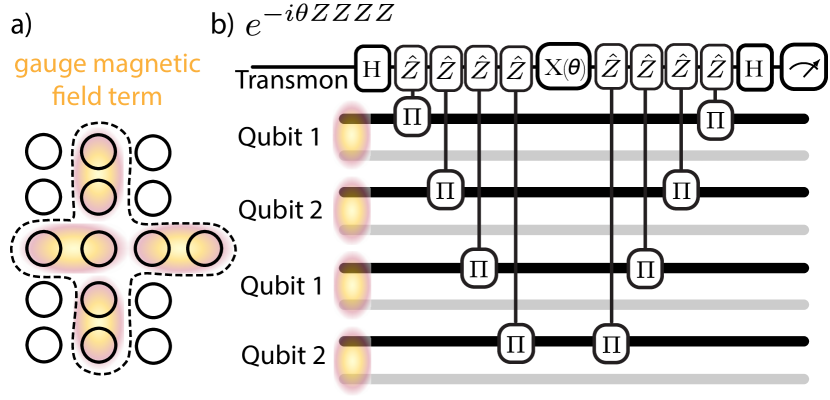
Figure 10: Dual rail magnetic field term $e^{\left(-i\theta\hat{Z}_{i,j}\hat{Z}_{j,k}\hat{Z}_{k,l}\hat{Z}_{l,i}\right)}$. a) Representation of the cavities taking part in the magnetic field term. b) Corresponding circuit. The gray and black colors of the mode wires correspond to the location of the boson when the dual-rail qubit is in state $\ket{0}$ or $\ket{1}$, respectively.

IV.2 Pure gauge dynamical $U(1)$ fields

Next, we turn to the $U(1)$ quantum link model described by the Hamiltonian in Eq. (3). As described in Sec. I.1, we utilize the Schwinger-boson representation to encode the link degrees of freedom, requiring two bosonic modes per link. We note that the Schwinger-boson representation may be understood as an extension of the dual-rail qubit encoding to spin $S>1/2$ [45].

IV.2.1 Electric field

In the Schwinger-Boson representation, the electric field energy can be written as

$$\hat{H}_{\mathrm{E}}=\frac{g^{2}}{2}\sum_{\braket{i,j}}\left(\frac{\hat{n}^{a}_{i,j}-\hat{n}^{b}_{i,j}}{2}-\frac{\tau}{2\pi}\right)^{2},$$ (72)

where $g$ is the strength of the electric field and $\tau$ here is the topological parameter. When multiplying out the square, the cross-Kerr terms $-\frac{g^{2}}{2}\hat{n}^{a}_{i,j}\hat{n}^{b}_{i,j}$ appear. Although we can in principle implement these terms, c.f. Sec. III.1.4, they are harder to implement than self-Kerr terms on the same site. Luckily, we can remove the cross-Kerr terms by using the Schwinger-Boson constraint $\hat{n}^{a}_{i,j}+\hat{n}^{b}_{i,j}=2S$. Due to this identity, we may add a term $\frac{g^{2}}{2}\sum_{i,j}\left(\frac{\hat{n}^{a}_{i,j}+\hat{n}^{b}_{i,j}}{2}\right)^{2}$, which due to the constraint is just a constant, to the Hamiltonian in Eq. (72) to obtain

$$\hat{H}_{\mathrm{E}} =\frac{g^{2}}{2}\sum_{\braket{i,j}}\left(\frac{1}{2}\left((\hat{n}^{a}_{i,j})^{2}+(\hat{n}^{b}_{i,j})^{2}\right)-\frac{\tau}{2\pi}(\hat{n}^{a}_{i,j}-\hat{n}^{b}_{i,j})\right)$$ (73)

$$\equiv\sum_{\braket{i,j}}\hat{h}_{E,i,j}$$ (74)

up to a constant, thereby removing the cross-Kerr term.

The time evolution under $\hat{H}_{E}$ fulfills $\exp(-i\hat{H}_{E}t)=\prod_{\braket{i,j}}\exp(-i\hat{h}_{E,i,j}t)$. Because the $\hat{a}$ and $\hat{b}$ modes commute, $\exp(-i\hat{h}_{E,i,j}t)=e^{-i\frac{g^{2}}{2}\left(\frac{1}{2}\hat{n}_{i,j}^{a^{2}}-\frac{\tau}{2\pi}\hat{n}^{a}_{i,j}\right)t}e^{-i\frac{g^{2}}{2}\left(\frac{1}{2}\hat{n}_{i,j}^{b^{2}}+\frac{\tau}{2\pi}\hat{n}^{b}_{i,j}\right)t}$. This can be implemented exactly using two $\operatorname{SNAP}(\vec{\theta})$ gates defined in Tab. 1 on modes $a$ and $b$:

$$\exp(-i\hat{h}_{E,i,j}t)=\operatorname{SNAP}_{a}(\vec{\theta}^{a})\operatorname{SNAP}_{b}(\vec{\theta}^{b})$$ (75)

where $\theta^{a}_{n}=\frac{g^{2}}{2}\left(\frac{1}{2}n^{2}-\frac{\tau}{2\pi}n\right)t$ and $\theta^{b}_{n}=\frac{g^{2}}{2}\left(\frac{1}{2}n^{2}+\frac{\tau}{2\pi}n\right)t$.

IV.2.2 Magnetic field

In $(2+1)\mathrm{D}$, the magnetic field Hamiltonian, illustrated in Fig. 11a, acts on the four gauge field raising operators linking a square (also called plaquette) of fermionic sites labelled $i,j,k,l$. We discuss the compilation of a single plaquette exponential term $\exp(-i\hat{H}_{\square}t)$ here, where

$$\hat{H}_{\square}= -\frac{1}{4g^{2}(S(S+1))^{2}}\left(\hat{S}^{+}_{i,j}\hat{S}^{+}_{j,k}\hat{S}^{-}_{k,l}\hat{S}^{-}_{l,i}+\mathrm{h.c.}\right).$$ (76)

Using our Schwinger-boson mapping of the gauge fields in Eq. (6), we obtain a product of creation and annihilation operators which we relabel $a,b$ for the modes of link $\langle i,j\rangle$, $c,d$ for link $\langle j,k\rangle$, $e,f$ for link $\langle k,l\rangle$ and $g,h$ for link $\langle l,i\rangle$ for simplicity of notation, such that:

$$\hat{H}_{\square}= -\frac{1}{4g^{2}(S(S+1))^{2}}\left(\hat{a}^{\dagger}\hat{b}\hat{c}^{\dagger}\hat{d}\hat{f}\hat{e}^{\dagger}\hat{h}\hat{g}^{\dagger}+\mathrm{h.c.}\right).$$ (77)

We show here how to realize the plaquette term using the method introduced in Ref. [102] and summarized in Sec. II.7, which makes use of the group commutator relations given by the Baker-Campbell-Hausdorff (BCH) formula, specifically the relation

$$e^{i\hat{A}\theta}e^{i\hat{B}\theta}e^{-i\hat{A}\theta}e^{-i\hat{B}\theta}=e^{-[\hat{A},\hat{B}]\theta^{2}+O\left(\theta^{3}\right)}.$$ (78)

Through appropriate choice of hybrid mode-qubit operators $\hat{A}$ and $\hat{B}$, this gives us the means to implement multiplication between commuting bosonic operators. We also use Trotter formulas to implement addition.

We rely on the above method and present a possible implementation that leverages the conditional beamsplitter gate introduced in Eq. (19) as the fundamental building block. This approach has the advantage of relying on simple hardware primitives, at the cost of Trotter error. Following this, we briefly comment on the possibility to instead leverage a three-wave mixing term realized on the hardware level, c.f. App. C. This latter approach would enable the compilation of the desired term without Trotter error, but uses a gate which is more complicated to engineer on the hardware level.

The key idea for this synthesis is to apply the BCH formula to conditional beamsplitters acting on the four pairs of modes around the plaquette, conditioned on the same ancillary qubit. Intuitively, this leads to multiplication of creation and annihilation operators for these four pairs of modes, yielding the eight-mode term in Eq. (77).

We first show how to synthesise a product of four mode operators. Choosing $e^{-i\hat{A}\theta}=\text{CBS}^{Y}_{a,b}(-\frac{\pi}{2},\theta)=e^{-i\theta(i\hat{a}^{\dagger}\hat{b}-i\hat{a}\hat{b}^{\dagger})\hat{Y}}$ and $e^{-i\hat{C}\theta}=\text{CBS}^{Z}_{c,d}(0,\theta)=e^{-i\theta(\hat{c}^{\dagger}\hat{d}+\hat{c}\hat{d}^{\dagger})\hat{Z}}$, where $\hat{H}$ is a Hadamard gate on the qubit and $\text{CBS}(\varphi,\theta)$ is defined in Eq. (19), we define the primitive

$$V(A\theta,C\theta)=e^{i\hat{A}\theta}e^{i\hat{C}\theta}e^{-i\hat{A}\theta}e^{-i\hat{C}\theta}.$$ (79)

This set of operations is illustrated in Fig. 11b. In order to reduce the error sufficiently, we use this primitive in a higher-order product formula [120]

$$\Gamma_{A,C}(\theta)$$

$$=V(A\gamma\theta,C\gamma\theta)V(-A\gamma\theta,-C\gamma\theta)V(C\gamma^{2}\theta,A\gamma^{2}\theta)$$

$$\times V(-C\gamma^{2}\theta,-A\gamma^{2}\theta)V(A\gamma\theta,C\gamma\theta)V(-A\gamma\theta,-C\gamma\theta)$$ (80)

$$=e^{-2\theta^{2}\left(\hat{a}^{\dagger}\hat{b}\hat{c}^{\dagger}d+\hat{a}^{\dagger}\hat{b}\hat{c}\hat{d}^{\dagger}-\hat{a}\hat{b}^{\dagger}\hat{c}^{\dagger}\hat{d}-\hat{a}\hat{b}^{\dagger}\hat{c}\hat{d}^{\dagger}\right)\otimes\hat{X}+\mathcal{O}\left(\theta^{5}\right)},$$ (81)

where $\gamma=1/\sqrt{4-2\sqrt{2}}$.

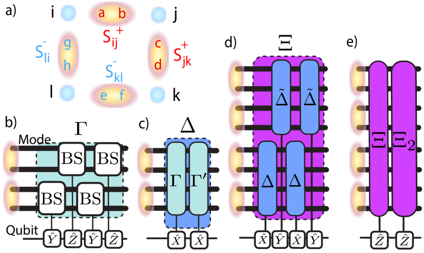
Figure 11: Baker-Campbell-Hausdorff synthesis of the plaquette term for the quantum link model in $(2+1)$D. a) BCH circuit corresponding to the creation of a qubit-conditional quartic term. b) Use of the Trotter formula to remove additional unwanted quartic terms. c) BCH circuit enabling the compilation of a term containing a multiplication of eight terms (octic). d) Final step in the circuit which uses the Trotter formula to remove unwanted octic terms. e) Representation of participating modes. The modes composing the gauge fields are labelled with letters $a$ through $g$, the matter fields are labelled $i$ through $l$. Depending on the geometry, not all $\operatorname{C\Pi}$ will be able to be directly conditioned on the same qubit, leading to the requirement for additional $\operatorname{SWAP}$ gates.

This expression contains two terms which are not part of the plaquette operator. In order to remove the unwanted terms, we apply the same four-mode synthesis again with different phases. This yields a new term $\Gamma_{A^{\prime},C^{\prime}}$ obtained using the primitive $V(A^{\prime}\theta,C^{\prime}\theta)$ with $e^{-i\hat{A}^{\prime}\theta}=\text{CBS}^{Y}_{a,b}(0,\theta)$ and $e^{-i\hat{C}^{\prime}\theta}=\text{CBS}^{Z}_{c,d}(-\frac{\pi}{2},\theta)$. Combining $\Gamma_{A,C}$ and $\Gamma_{A^{\prime},C^{\prime}}$ in a second-order Trotter formula, we remove the unwanted terms,

$$\Delta_{A,C} =\Gamma_{A,C}(\theta/2)\Gamma_{A^{\prime},C^{\prime}}(\theta)\Gamma_{A,C}(\theta/2)$$

$$=e^{\left(\left(-2i\hat{a}^{\dagger}\hat{b}\hat{c}^{\dagger}\hat{d}+2i\hat{a}\hat{b}^{\dagger}\hat{c}\hat{d}^{\dagger}\right)\otimes 2iX\right)(-i\theta)^{2}}+\mathcal{O}\left(\theta^{5}\right),$$ (82)

This set of operations is illustrated in Fig. 11c and we dropped the $\mathcal{O}(\theta^{6})$ Trotter error as the $\mathcal{O}(\theta^{5})$ BCH error dominates. Using a single-qubit gate on the qubit, one can also obtain $(\Delta_{A,C})^{\dagger}$. The same expression can be obtained on the other four modes which are also involved in the plaquette term:

$$\tilde{\Delta}_{E,G}=e^{\left(\left(-2i\hat{e}^{\dagger}\hat{f}\hat{g}^{\dagger}\hat{h}+2i\hat{e}\hat{f}^{\dagger}\hat{g}\hat{h}^{\dagger}\right)\otimes 2i\hat{Y}\right)(-i\theta)^{2}+\mathcal{O}\left(\theta^{5}\right)}.$$ (83)

Note that $\tilde{\Delta}_{E,G}$ is chosen such that $\hat{Y}$ is carried out on the qubit rather than $\hat{X}$ – this is to enable the further use of the BCH formula which we explain next.

In order to obtain the eight-wave mixing required to realise the plaquette term, we concatenate four four-mode terms according to

$$\Xi_{\{A,C\},\{E,G\}}=\Delta_{A,C}\tilde{\Delta}_{E,G}\Delta_{A,C}^{\dagger}\tilde{\Delta}_{E,G}^{\dagger}.$$ (84)

This set of operations is illustrated in Fig. 11d. Similarly to the four-mode term, equation (84) yields terms which are not part of the plaquette term. In order to remove them, we multiply $\Xi_{\{A,C\},\{E,G\}}$ with a term which is obtained in the same way but with a different choice of phases in the beamsplitters:

$$\Xi_{2,\{A_{2},C_{2}\},\{E_{2},G_{2}\}}=\Delta_{A_{2},C_{2}}\tilde{\Delta}_{E_{2},G_{2}}\Delta^{\dagger}_{A_{2},C_{2}}\tilde{\Delta}^{\dagger}_{E_{2},G_{2}}.$$ (85)

The constituent operations part of this term are the following, where we use the same notation with primes and tildes as in the discussion of the synthesis of $\Xi_{\{A,C\},\{E,G\}}$. On modes $a,b,c,d$ we use

$${A}_{2} =\hat{H}\>\text{CBS}_{a,b}\left(\pi,1\right)\>\hat{H},$$ (86)

$${C}_{2} =\text{CBS}_{c,d}\left(0,1\right),$$ (87)

$${A^{\prime}}_{2} =\hat{H}\>\text{CBS}_{a,b}\left(\frac{\pi}{2},1\right)\>\hat{H},$$ (88)

$${C^{\prime}}_{2} =\text{CBS}_{c,d}\left(\frac{\pi}{2},1\right).$$ (89)

On modes $e,f,g,h$ we use

$$\tilde{E}_{2} =\hat{H}\>\text{CBS}_{a,b}(0,1)\>\hat{H},$$ (90)

$$\tilde{G}_{2} =\hat{H}\>\hat{S}\>\text{CBS}_{c,d}(0,1)\hat{H}\>\hat{S}^{\dagger},$$ (91)

$$\tilde{E^{\prime}}_{2} =\hat{H}\>\text{CBS}_{a,b}\left(\frac{\pi}{2},1\right)\>\hat{H},$$ (92)

$$\tilde{G^{\prime}}_{2} =\hat{H}\>\hat{S}\>\text{CBS}_{c,d}\left(-\frac{\pi}{2},1\right)\hat{H}\>\hat{S}^{\dagger}.$$ (93)

In total, we obtain

$$\Xi_{\{A,C\},\{E,G\}}\Xi_{2,\{A_{2},C_{2}\},\{E_{2},G_{2}\}}=$$ (94)

$$e^{-i\left(16\left(\hat{a}^{\dagger}\hat{b}\hat{c}^{\dagger}\hat{d}\hat{f}\hat{e}^{\dagger}\hat{h}\hat{g}^{\dagger}+\hat{a}\hat{b}^{\dagger}\hat{c}\hat{d}^{\dagger}\hat{f}^{\dagger}\hat{e}\hat{h}^{\dagger}\hat{g}\right)\otimes\hat{Z}\right)\theta^{4}+O\left(\theta^{5}\right)},$$ (95)

illustrated in Fig. 11e. Choosing $\theta=\left(\frac{1}{64g^{2}(S(S+1))^{2}}t\right)^{1/4}$ we get time evolution under a single plaquette Hamiltonian for a timestep $t$. Each CBS gate can be implemented using $2$ conditional parity operations and $1$ beamsplitter, c.f. Eq. (19). We count conditional parities in the following. Each $\Gamma$ can be implemented using $6$ $V$ operations (see Eq. (79)), which require $8$ conditional parities to implement and hence each $\Gamma$ requires $48$ conditional parities. Each $\Delta$ operation requires $3$ $\Gamma$ operations using the symmetric Trotter formula implying that it requires $144$ conditional parities. Each $\Xi$ is built from $4$ $\Delta$ terms and hence each requires $576$ conditional parities. Then the final approximation, $V_{\square}$ requires $1152$ conditional parities as it is composed of two $\Xi$ operations.

We close with a discussion of the error term. Because each pair of mode operators has norm $\|a^{\dagger}b\|=\sqrt{S(S+1)}$ in the Schwinger-boson encoding of a large spin and the error term contains $5$ such pairs, our result implies that the distance between the thus-implemented unitary $V_{\square}$ and the exact plaquette exponential is

$$\left\|V_{\square}-e^{-i\left(16\left(\hat{a}^{\dagger}\hat{b}\hat{c}^{\dagger}\hat{d}\hat{f}\hat{e}^{\dagger}\hat{h}\hat{g}^{\dagger}+\hat{a}\hat{b}^{\dagger}\hat{c}\hat{d}^{\dagger}\hat{f}^{\dagger}\hat{e}\hat{h}^{\dagger}\hat{g}\right)\otimes\hat{Z}\right)t}\right\|$$

$$\quad=\mathcal{O}\left(\frac{t^{5/4}}{g^{5/2}}\right).$$ (96)

In particular, this error is independent of $S$.

Another way of synthesising this term would be to use the three-wave mixing term introduced in App. C. Because the additional terms appearing in the beamsplitter approach mentioned above would not appear using three-wave mixing, we could save on Trotter error and reduce the number of native operations needed by a prefactor. However, because the Trotter error is sub-leading, this will not change the asymptotic error scaling shown above.

$\hat{H}$	$e^{-i\hat{H}t}$ Intermediary Step	$\quad\quad\quad\quad\quad\quad e^{-i\hat{H}t}$ Gates	Definition
Bosons $\sum\limits_{\braket{i,j}}J_{i,j}\left(\hat{a}^{\dagger}_{i}\hat{U}_{i,j}\hat{a}_{j}+\mathrm{h.c.}\right)$	$\mathbb{Z}_{2}$ $\exp\left(-iJ_{i,j}t\left(\hat{a}^{\dagger}_{i}Z_{i,j}\hat{a}_{j}+\mathrm{h.c.}\right)\right)$	Transmon $\mathbb{Z}_{2}$ $\operatorname{C\Pi}_{i,j}$, $\operatorname{BS}_{i,j}(\varphi,\theta)$ Dual Rail $\mathbb{Z}_{2}$ $\operatorname{C\Pi}_{i,j}$, $\operatorname{BS}_{i,j}(\varphi,\theta)$, $\operatorname{SQR}_{i,j}(\theta)\quad\quad\quad\quad\quad$	Sec. IV.4.1
	$U(1)$ $\exp\left(-iJ_{i,j}t\left(\hat{a}^{\dagger}_{i}\hat{a}^{\dagger}_{i,j}\hat{b}_{i,j}\hat{a}_{j}+\mathrm{h.c.}\right)\right)$	Dual Rail $U(1)$ $\>\operatorname{BS}_{i,j}(\varphi,\theta)$, $\operatorname{C\Pi}$, $\operatorname{R^{\varphi}_{i}(\theta)}$	Sec. IV.5.1
Fermions $\sum\limits_{\braket{i,j}}J_{i,j}\left(\hat{c}^{\dagger}_{i}\hat{U}_{i,j}\hat{c}_{j}+\mathrm{h.c.}\right)$	$\mathbb{Z}_{2}$ $\quad(1)\>\operatorname{SWAP}$, $\operatorname{FSWAP}$ $(2)\>\exp\left(-iJ_{i,j}t\left(\hat{\sigma}^{+}_{i}\hat{Z}_{i,j}\hat{\sigma}^{-}_{j}+\mathrm{h.c.}\right)\right)$	Transmon $\mathbb{Z}_{2}$ & Dual Rail Fermions $(1)\>\operatorname{SWAP}_{i,j}$, $\operatorname{C\Pi}_{i,j}$, $\operatorname{R^{\varphi}}_{i}(\theta)$, $\operatorname{R}_{i}(\theta)$ $(2)\>\operatorname{BS}_{i,j}(\varphi,\theta)$, $\operatorname{C\Pi}_{i,j}$, $\operatorname{R^{\varphi}}_{i}(\theta)$	Sec. IV.4.2
	$U(1)$ $(1)\>\operatorname{SWAP}$, $\operatorname{FSWAP}$ $(2)\>\exp\left(-iJ_{i,j}t\left(\hat{\sigma}^{+}_{i}\hat{a}^{\dagger}_{i,j}\hat{b}_{i,j}\hat{\sigma}^{-}_{j}+\mathrm{h.c.}\right)\right)$	Dual Rail Gauge & Transmon Fermions $(1)\>\operatorname{SWAP}_{i,j},\operatorname{CD}_{i,j}(\theta),\operatorname{R}^{Z}_{i}(\theta)$ $(2)\>\operatorname{C\Pi}_{i,j}$, $e^{i\theta\hat{E}}$, $e^{i\theta\hat{F}}$, $\operatorname{R^{\varphi}_{i}(\theta)}$	Sec. IV.5.2
		Dual Rail Gauge & Dual Rail Fermions $\>\operatorname{SWAP}_{i,j}$, $\operatorname{CR_{i,j}(\theta)}$, $\operatorname{R^{\varphi}_{i}(\theta)}$ $(2)\>\operatorname{BS}_{i,j}(\varphi,\theta)$, $\operatorname{C\Pi}$, $\operatorname{R^{\varphi}_{i}(\theta)}$	Sec. IV.5.2

Table 6: Compilation strategy for gauge-invariant hopping Hamiltonian terms into the native gates in the proposed architecture (see Fig. 2). We use $\hat{U}_{i,j}$ as a placeholder for a parallel transporter.

IV.3 Static gauge fields coupled to matter

Static gauge fields appear when a magnetic field [111] is coupled to matter and are crucial when, for example, considering the fractional quantum Hall effect [112]. In this case, the hopping term of the Hamiltonian has a fixed complex amplitude on each link, i.e.,

$$-J\sum\limits_{\braket{i,j}}\left(e^{i\varphi}\hat{a}^{\dagger}_{i}\hat{a}_{j}+\mathrm{h.c.}\right),$$ (97)

where we have specialized to the case of bosonic matter. This term can be directly implemented by a beamsplitter $\text{BS}_{i,j}(\varphi,\theta)$ defined in Tab. 1 via the appropriate choice for the phase $\varphi$ for each link.

For fermionic matter, the hopping term generalizes as

$$-J\sum\limits_{\braket{i,j}}\left(e^{i\varphi}\hat{c}^{\dagger}_{i}\hat{c}_{j}+\mathrm{h.c.}\right).$$ (98)

The phase can be implemented as a part of the gates necessary for the Jordan-Wigner encoding described in App. A.1, for either choice of qubit type. The $\operatorname{FSWAP}$ operation would remain unchanged, but the phase can be incorporated by conjugating the fermionic hopping by $e^{i\varphi\hat{Z}}$ on one of the qubits.

IV.4 Dynamical $\mathbb{Z}_{2}$ fields coupled to matter

Here we discuss $\mathbb{Z}_{2}$-Higgs model gauge fields coupled to bosonic and fermionic matter. We first discuss the bosonic gauge-invariant hopping in Sec. IV.4.1, mapping the gauge fields to transmon and then dual rail qubits. We then discuss the fermionic gauge-invariant hopping in Sec. IV.4.2, mapping the fermions and the gauge fields to transmon and dual rail qubits.

IV.4.1 Bosonic gauge-invariant hopping

The time evolution operator of the gauge-invariant bosonic hopping mediated by a $\mathbb{Z}_{2}$ gauge field takes the form

$$e^{-it\hat{Z}_{i,j}\left(\hat{a}^{\dagger}_{i}\hat{a}_{j}+\hat{a}_{i}\hat{a}^{\dagger}_{j}\right)}.$$ (99)

In the following, we discuss the implementation of this operator using either transmons or dual rail (DR) qubits. For both cases, we use modes to directly encode the bosonic matter.

Field: transmons $|$ Matter: modes. For the situation where we map the gauge fields onto transmon qubits, Eq. (99) corresponds to a conditional beamsplitter, discussed in Sec. II.2.

Field: dual rail $|$ Matter: modes. For the case where we map the gauge fields onto dual-rail qubits, we leverage the fact that the parity of the photon number $\hat{n}$ in one of the rails is equivalent to the Pauli operator $\hat{Z}^{\textrm{DR}}$ (see Eq. (59)). Therefore the time evolution of the hopping between sites $i$ and $j$ takes the form

$$e^{-ite^{i\pi\hat{n}_{i,j}}\left(a_{i}^{\dagger}a_{j}+\hat{a}_{i}\hat{a}^{\dagger}_{j}\right)}.$$ (100)

and can be compiled using the methods described in Sec. II.3 and shown in Fig. 12.

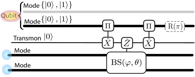
Figure 12: $\mathbb{Z}_{2}$ Gauge-invariant hopping circuit. Implementation of the gauge-invariant hopping with dual rail qubits as $\mathbb{Z}_{2}$ gauge fields and modes as the matter sites: $e^{-i\theta e^{i\pi\hat{n}_{i,j}}\left(e^{i\varphi}a_{i}^{\dagger}a_{j}+\mathrm{h.c.}\right)}$. The gray and black colors of the mode wires participating in the dual rail qubit (two upper modes) correspond to the location of the boson when the dual-rail qubit is in state $\ket{0}$ or $\ket{1}$, respectively. The beamsplitter is conditioned on $\hat{Z}$.

IV.4.2 Fermionic gauge-invariant hopping

The fermionic SWAP networks used to implement fermionic gauge-invariant hopping require the exact same FSWAP operations as are discussed in App. A.1, where the gauge field also needs to be swapped. To make the hopping gauge invariant, we replace the iSWAP operation with

$$e^{-it(-J)\hat{Z}_{i,j}\left(\hat{X}_{i}\hat{X}_{j}+\hat{Y}_{i}\hat{Y}_{j}\right)}$$

$$=e^{-it(-J)\hat{Z}_{i,j}\left(\hat{X}_{i}\hat{X}_{j}\right)}e^{-it(-J)\hat{Z}_{i,j}\left(\hat{Y}_{i}\hat{Y}_{j}\right)}$$

$$= \operatorname{R}^{\frac{\pi}{2}}_{i}\left(\frac{\pi}{2}\right)\operatorname{R}^{\frac{\pi}{2}}_{j}\left(\frac{\pi}{2}\right)e^{-it(-J)\hat{Z}_{i,j}\left(\hat{Z}_{i}\hat{Z}_{j}\right)}\operatorname{R}^{\frac{\pi}{2}}_{i}\left(-\frac{\pi}{2}\right)\operatorname{R}^{\frac{\pi}{2}}_{j}\left(-\frac{\pi}{2}\right)$$

$$\times \operatorname{R}^{0}_{i}\left(\frac{\pi}{2}\right)\operatorname{R}^{0}_{j}\left(\frac{\pi}{2}\right)e^{-it(-J)\hat{Z}_{i,j}\left(\hat{Z}_{i}\hat{Z}_{j}\right)}\operatorname{R}^{0}_{i}\left(-\frac{\pi}{2}\right)\operatorname{R}^{0}_{j}\left(-\frac{\pi}{2}\right),$$ (101)

using the fact that $\hat{X}=\operatorname{R}^{\frac{\pi}{2}}(\pi/2)\hat{Z}\operatorname{R}^{\frac{\pi}{2}}(-\pi/2)$ and $\hat{Y}=\operatorname{R}^{\pi}(\pi/2)\hat{Z}\operatorname{R}^{\pi}(-\pi/2)$, where $\operatorname{R}^{\varphi}(\theta)$ is defined in Tab. 1. We note that this gate sequence can be further compressed by combining successive single-qubit gates into a single rotation.

We do not discuss the all-transmon qubit implementation of this model as this case does not leverage the advantages of our platform.

Field: transmon $|$ Matter: dual rail. Following Eq. (101), single-qubit rotations can be performed on the dual rail qubits using beamsplitter gates, while $e^{-it(-J)\hat{Z}_{i,j}\left(\hat{Z}_{i}^{\textrm{DR}}\hat{Z}_{j}^{\textrm{DR}}\right)}$ is a transmon $Z$-conditional dual rail $\operatorname{ZZ}^{\textrm{DR}}$ operation. This latter gate is compiled in Eq. (64) using an ancillary transmon initialized to $\ket{0}_{\textrm{anc}}$ that is ultimately traced out. However, we can adapt this same sequence to realize the desired gate by replacing the ancilla with the transmon encoding the gauge field in an unknown state (and removing the matrix element projection in Eq. (64)).

Field: dual rail $|$ Matter: transmon. This term requires the implementation of $e^{-it(-J)e^{i\pi\hat{n}_{i,j}}\left(\hat{X}_{i}\hat{X}_{j}+\hat{Y}_{i}\hat{Y}_{j}\right)}=e^{-it(-J)e^{i\pi\hat{n}_{i,j}}\hat{X}_{i}\hat{X}_{j}}e^{it(-J)e^{-i\pi\hat{n}_{i,j}}\hat{Y}_{i}\hat{Y}_{j}}$ which can be implemented using additional single-qubit rotations from $e^{-i\theta e^{i\pi\hat{n}_{i,j}}\hat{Z}_{i}\hat{Z}_{j}}$. The latter is an instance of the parity-controlled gate $\operatorname{CU}^{\bar{\Pi}}_{i,j}$ introduced in Sec. II.3. Specifically, the intermediate gate in Eq, (30) would be replaced by the two transmon qubit gate $\operatorname{ZZ}(\theta)$ implemented in our architecture via the technique in Sec. II.6.

Field: dual rail $|$ Matter: dual rail. Following Eq. (101), aside from single-qubit rotations, we require implementation of $e^{-it(-J)\hat{Z}_{i,j}^{\textrm{DR}}\left(\hat{Z}_{i}^{\textrm{DR}}\hat{Z}_{j}^{\textrm{DR}}\right)}$. This type of multi dual-rail gate can be realized using the Pauli-exponentiation gadget as discussed in Sec. IV.1.2 and shown in Fig. 10, there for the slightly more complex case of four dual-rail qubits. Alternatively, one can iterate the parity-control synthesis technique of Sec. II.3, similar to the doubly-conditional displacement realized in Eq. (71).

IV.5 Dynamical $U(1)$ fields coupled to matter

Next, we discuss the implementation of dynamical $U(1)$ fields coupled to bosonic (Sec. IV.5.1) and fermionic matter (Sec. IV.5.2). We show how to implement the dynamics of the hopping described in Eq. (3) which has the form:

$$\exp\left(-i\frac{Jt}{2\sqrt{S(S+1)}}\sum_{\braket{i,j}}\left(\hat{m}^{\dagger}_{i}\hat{S}^{+}_{i,j}\hat{m}_{j}+\mathrm{h.c.}\right)\right).$$ (102)

In the remainder of the section, we will assume large $S$ and write $\sqrt{S(S+1)}\approx S$. As in Sec. IV.2, we leverage the Schwinger-boson encoding the represent the $U(1)$ gauge fields. Furthermore, for the case of fermionic matter, we separately consider transmons and dual-rail qubits.

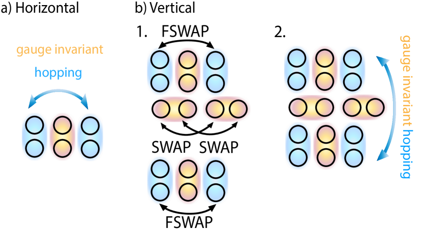
Figure 13: Gauge-invariant hopping of fermions across $U(1)$ gauge fields. a) Horizontal hopping. It only requires a nearest-neighbour gauge-invariant hopping operation where fermion operators are replaced with qubit operators. b) Vertical hopping. FSWAP networks are generalized by first SWAPing the gauge field modes at the same time as performing FSWAPs and then applying the same operation as for the horizontal hopping on the vertical bond. The gauge field modes involved in the horizontal hoppings are left unchanged.

IV.5.1 Bosonic gauge-invariant hopping

For a bosonic matter site $i$ denoted by operator $\hat{d}$, the gauge-invariant hopping between site $i$ and site $j$ is given by

$$e^{-i\,t\,\frac{J}{2S}\left(\hat{d}^{\dagger}_{i}\hat{a}^{\dagger}_{i,j}\hat{b}^{\phantom{\dagger}}_{i,j}\hat{d}^{\phantom{\dagger}}_{j}+\mathrm{h.c.}\right)},$$ (103)

where $\hat{a}^{\dagger}_{i,j}\hat{b}^{\phantom{\dagger}}_{i,j}$ is the Schwinger boson representation of the link operator $\hat{S}^{+}_{i,j}$. This unitary is generated by a four-mode mixing term, and can be synthesized using the BCH formula, see Eq. (54).

IV.5.2 Fermionic gauge-invariant hopping

For fermions in $(2+1)$D, we first use FSWAP networks to move the sites to neighbouring sites within the JW encoding. To then perform the gauge-invariant hopping, we also SWAP the corresponding gauge fields as depicted in Fig. 13. The remaining operation is then given by the nearest-neighbour hopping

$$e^{-i\,t\,\frac{J}{2S}\left(\hat{\sigma}^{+}_{i}\hat{a}^{\dagger}_{i,j}\hat{b}^{\phantom{\dagger}}_{i,j}\hat{\sigma}^{-}_{j}+\mathrm{h.c.}\right)},$$ (104)

where $j$ is a neighbouring site to $i$. In $(1+1)$D, SWAP and FSWAP operations are not necessary. We now discuss how this term is synthesized for the cases where the fermions are encoded in transmons or dual-rail qubits.

Fermionic matter: transmons. We present two schemes, a naive implementation which contains Trotter error, and a scheme which avoids Trotter error (for this term alone), but requires a particular experimental adaptation of the hardware.

Scheme 1 – We rewrite the gauge-invariant hopping term as

$$e^{-i\frac{Jt}{2S}(\hat{H}_{1}+\hat{H}_{2})}\approx e^{-i\frac{Jt}{2S}\hat{H}_{1}}e^{-i\frac{Jt}{2S}\hat{H}_{2}}+\mathcal{O}\left(\left(\frac{Jt}{2S}\right)^{2}\right),$$ (105)

where we used Trotterization and defined

$$\hat{H}_{1} =\left(\hat{X}_{i}\hat{X}_{j}+\hat{Y}_{i}\hat{Y}_{j}\right)\left(\hat{a}^{\dagger}_{i,j}\hat{b}_{i,j}+\mathrm{h.c.}\right)$$ (106)

$$\hat{H}_{2} =\left(\hat{Y}_{i}\hat{X}_{j}-\hat{X}_{i}\hat{Y}_{j}\right)\left(e^{i\pi/2}\hat{a}^{\dagger}_{i,j}\hat{b}_{i,j}+\mathrm{h.c.}\right).$$ (107)

Noting that $\hat{X}_{i}\hat{X}_{j}$ and $\hat{Y}_{i}\hat{Y}_{j}$ commute, as do $\hat{Y}_{i}\hat{X}_{j}$ and $\hat{X}_{i}\hat{Y}_{j}$, we are then left with implementing doubly conditional beamsplitters. This is done by sandwiching a beamsplitter with conditional parity operations conditioned on the qubits $i$ and $j$, as shown in Eq. (19). However, $[\hat{H}_{1},\hat{H}_{2}]\neq 0$ and this term will therefore acquire Trotter error.

Scheme 2 – This scheme does not introduce Trotter error, but requires additional engineering at the hardware level. We define the unitary as $e^{-i\theta\hat{H}}$ with $\hat{H}=\sigma_{i}^{+}a^{\dagger}b\sigma_{j}^{-}+\sigma_{i}^{-}ab^{\dagger}\sigma_{j}^{+}$ where, for simplicity we have dropped the indices ${i,j}$ on the modes $a$ and $b$ and we defined $\theta=\frac{Jt}{2S}$. We start by breaking up $\hat{H}$ into $\hat{H}=\hat{C}+\hat{D}$, where

$$\hat{C} =\hat{X}_{i}\left(\hat{X}_{j}\left(a^{\dagger}b+ab^{\dagger}\right)+i\hat{Y}_{j}\left(a^{\dagger}b-ab^{\dagger}\right)\right)/4$$

$$\equiv\hat{X}_{i}\hat{E}_{j}$$ (108)

$$\hat{D} =\hat{Y}_{i}\left(-i\hat{X}_{j}\left(a^{\dagger}b-ab^{\dagger}\right)+\hat{Y}_{j}\left(a^{\dagger}b+ab^{\dagger}\right)\right)/4$$

$$\equiv\hat{Y}_{i}\hat{F}_{j}.$$ (109)

Indeed, $\left[\hat{C},\hat{D}\right]=0$ because $\{\hat{E}_{j},\hat{F}_{j}\}=0$.

It is helpful to rewrite:

$$\hat{E}_{j} =\left(ab^{\dagger}\sigma_{j}^{+}+a^{\dagger}b\sigma_{j}^{-}\right)/2$$ (110)

$$\hat{F}_{j} =i\left(ab^{\dagger}\sigma_{j}^{+}-a^{\dagger}b\sigma_{j}^{-}\right)/2.$$ (111)

With this, we can now express the desired time-evolution operator as

$$e^{-i\theta\hat{H}} =e^{-i\theta\hat{D}}e^{-i\theta\hat{C}}$$

$$=e^{-i\theta\hat{Y}_{i}\hat{F}_{j}}e^{-i\theta\hat{X}_{i}\hat{E}_{j}}$$

$$=R^{0}_{i}\left(-\frac{\pi}{2}\right)\mathrm{C\Pi}_{i,j}e^{-i\theta\hat{F}}\mathrm{C\Pi}_{i,j}R^{0}_{i}\left(\frac{\pi}{2}\right)$$

$$\times R^{\frac{\pi}{2}}_{i}\left(-\frac{\pi}{2}\right)\mathrm{C\Pi}_{i,j}e^{-i\theta\hat{E}}\mathrm{C\Pi}_{i,j}R^{\frac{\pi}{2}}_{i}\left(\frac{\pi}{2}\right),$$ (112)

where $R^{\varphi}(\theta)$ (a single transmon qubit rotation gate) and $\operatorname{C\Pi}$ gates are defined in Tab. 1. This reduces the problem of realizing four-body interactions to the more manageable problem of realizing the three-body interaction Hamiltonians – the latter being more natural to realize in the circuit QED architecture given the primary source of non-linearity is the four-wave mixing property of Josephson junctions. We derive one possible implementation of these interactions in App. C.

Fermionic matter: dual-rail. In this case, we must implement a many-body gate that involves the two Schwinger-boson modes representing the gauge fields $a_{i,j}$ and $b_{i,j}$, and the four modes composing the two dual-rail qubits $c_{i},d_{i}$ and $c_{j},d_{j}$:

$$e^{-i\theta\left(\hat{c}_{i}^{\dagger}\hat{d}_{i}\hat{a}^{\dagger}_{i,j}\hat{b}^{\phantom{\dagger}}_{i,j}\hat{c}_{j}\hat{d}_{j}^{\dagger}+\mathrm{h.c.}\right).}$$ (113)

To implement such a gate, we use the BCH formula synthesis methods presented in Sec. IV.2.2 for pure $U(1)$ gauge fields. In particular, we apply Eq. (52), where we set $e^{i\hat{X}\hat{O}_{1}\theta}=e^{\left(\left(-2ic_{i}^{\dagger}d_{i}a_{i,j}^{\dagger}b_{i,j}+2ic_{i}d_{i}^{\dagger}a_{i,j}b_{i,j}^{\dagger}\right)\otimes 2iX\right)(-i\theta)^{2}+O\left(\theta^{3}\right)}$ for which the compilation was shown in Eq. (82), and set $e^{i\hat{Y}\hat{O}_{2}\theta}=e^{-i\hat{Y}_{k}\left(c_{j}^{\dagger}d_{j}+\mathrm{h.c.}\right)\theta}$. This yields unwanted terms which we cancel using the Trotter formula in Eq. (53) through use of BCH with appropriate phases in the beamsplitters.

V Gate complexity and comparison to all-qubit algorithms 

In this section, we analyse the gate complexity of our qubit-boson Trotter approach. In particular, we discuss the interplay of Trotter errors with errors introduced by some of our compilation schemes. We first review the general principles of Trotter error analysis. We then discuss a particular Trotter implementation of the $\mathbb{Z}_{2}$-Higgs model and $U(1)$ quantum link model and its error. While all compilations are exact for the $\mathbb{Z}_{2}$-Higgs model, the compilation of the magnetic field term in the $U(1)$ quantum link model (c.f. section IV.2.2) introduces additional error. We therefore discuss the interplay of Trotter error with this compilation error. While these sections focus on the asymptotic scaling of the whole Trotter algorithm, we close the section with a comparison of the explicit gate counts of a single Trotter step in our qubit-boson approach and compare it to an all-qubit approach. To do so, we introduce a qubit algorithm for simulating beamsplitters between bosonic modes.

V.1 General Trotter error analysis

We write the Hamiltonian as a sum of terms $\hat{H}=\sum_{\gamma=1}^{\Gamma}\hat{H}_{\gamma}$. We first decompose the time evolution $\exp\left(-i\hat{H}T\right)$ until time $T$ into $r$ time steps of duration $t=T/r$, i.e. $\exp\left(-i\hat{H}T\right)=\left(\exp\left(-i\hat{H}t\right)\right)^{r}$. An estimate of the error

$$\epsilon_{\mathrm{Trotter}}\equiv\|(\mathcal{S}(t))^{r}-e^{-i\hat{H}T}\|$$ (114)

of a $2$p-th order Trotter formula $\mathcal{S}(t)$ as introduced in section I.3 is [121]

$$\epsilon_{\mathrm{Trotter}}=\mathcal{O}\left(\left(\sum_{\gamma}\|\hat{H}_{\gamma}\|\right)^{2p+1}\frac{T^{2p+1}}{r^{2p}}\right).$$ (115)

The number of Trotter steps for a target Trotter error is hence

$$r =\mathcal{O}\left(\left(\sum_{\gamma}\|\hat{H}_{\gamma}\|\right)^{\frac{2p+1}{2p}}\frac{T^{\frac{2p+1}{2p}}}{\epsilon_{\mathrm{Trotter}}^{\frac{1}{2p}}}\right)$$ (116)

$$=\mathcal{O}\left(\left(\sum_{\gamma}\|\hat{H}_{\gamma}\|T\right)^{1+\frac{1}{2p}}\epsilon_{\mathrm{Trotter}}^{-\frac{1}{2p}}\right).$$ (117)

From this expression, we get the total number of gates as

$$N_{\mathrm{gates},2p} =r5^{p-1}N_{\mathrm{gates},2p=2}$$ (118)

$$=r5^{p-1}2\sum_{\gamma}N_{\mathrm{gates,\gamma}},$$ (119)

where $N_{\mathrm{gates,\gamma}}$ is the number of gates required for the individual exponentials $\exp(-i\hat{H}_{\gamma}t)$. We used that a Trotter formula of order $2p$ requires $5$ times the number gates of a Trotter formula of order $2p-2$ when defined recursively [121]. The second-order Trotter formula requires twice as many gates as the first-order Trotter formula. Finally, the number of gates required for the first-order Trotter formula is the sum of the number of gates $N_{\gamma}$ required for each exponential. In cases where the individual exponentials can only be synthesized with error (dependent on $t$), $N_{\mathrm{gates,\gamma}}$ contributes to the overall complexity. Note that in general, the complexity of Trotter formulas is evaluated at fixed $p$. Hence, factors such as $5^{p-1}$ above are dropped for estimating the asymptotic complexity in $\mathcal{O}$ notation.

Approximating the Trotter error in terms of the norms of the Hamiltonian terms overestimates the error because most terms in many-body Hamiltonians commute with each other. We therefore expect the Trotter error to be much smaller in practice, see e.g. [122] for a tighter estimate for the $(1+1)$D fermionic $U(1)$ quantum link model.

Bosonic Hamiltonians have an in-principle unbounded norm and therefore naively exhibit an unbounded product-formula error. However, in practice, infinitely high Fock states are not occupied during the dynamics such that the error stays bounded. In particular, in the $U(1)$ quantum link model, the spectral norm of bosonic operators is bounded by $\sqrt{S}$. Similarly, in the $\mathbb{Z}_{2}$-Higgs model, using an initial state with a total number of $N$ bosons in the system, bosonic operators are bounded by $\sqrt{N}$.

We detail specific Trotter decompositions of the $U(1)$ quantum link model and $\mathbb{Z}_{2}$-Higgs model and their errors next. We specifiy to open boundary conditions on an $L\times L$ square lattice and use the triangle inequality $\|\hat{H}_{0}+\hat{H}_{1}\|\leq\|\hat{H}_{0}\|+\|\hat{H}_{1}\|$ as well as $\|a\hat{H}_{0}\|=|a|\|\hat{H}_{0}\|$. For bosonic matter, we assume evolution within a sector of total boson number $N$ to estimate the Trotter error.

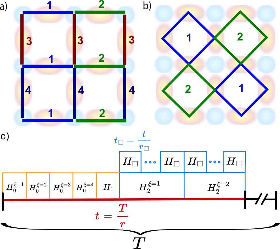
Figure 14: Illustration of the Trotter decomposition. a) Gauge-invariant hopping. It is split into four components $\xi=1,2,3,4$ such that all terms within the component commute. b) Plaquette term. We split the square lattice into two disjoint checkerboard patterns. In both subfigures, the numbers correspond to the $\xi$ indices. c) Illustration of the partition of time evolution until time $T$ into different sub-Hamiltonians. For the $\mathbb{Z}_{2}$-Higgs model ((120)-(124)) a further decomposition of (124) into $r_{\square}$ evolutions under $H_{\square}$ is not necessary, but it is for (132) of the $U(1)$ quantum link model ((128)-(132)).

V.2 Trotter decomposition and gate complexity of the $\mathbb{Z}_{2}$-Higgs model

The electric field and on-site interaction term commute with each other such that we can choose

$$\hat{H}_{0}=-g\sum_{\braket{i,j}}\hat{X}_{i,j}+U\sum_{i=1}^{L^{2}}\hat{n}_{i}^{2},$$ (120)

where $\braket{i,j}$ indicates summation over the $2L(L-1)$ bonds on a square lattice with $L^{2}$ sites. It follows from the triangle inequality and $\|\hat{X}_{i}\|=1$, $\|\hat{n}_{i}\|=N$ in a fixed particle sector with $N$ particles that

$$\|\hat{H}_{0}\|\leq 2gL(L-1)+|U|L^{2}N^{2}.$$ (121)

Next, we split the gauge-invariant hopping into four non-commuting terms $\xi=1,2,3,4$, where $1(2)$ denote the even(odd) hoppings in the horizontal direction and $3(4)$ the even(odd) hoppings in the vertical direction, c.f. Fig. 14a). We write this as

$$\hat{H}_{1}^{\xi}=-J\sum_{\braket{i,j}_{\xi}}\left(\hat{m}^{\dagger}_{i}\hat{Z}_{i,j}\hat{m}_{j}+\mathrm{h.c.}\right).$$ (122)

Next we find $\|\hat{m}^{\dagger}_{i}\hat{Z}_{i,j}\hat{m}_{j}+\mathrm{h.c.}\|\leq 2\|\hat{m}^{\dagger}_{i}\|\|\hat{Z}_{i,j}\|\|\hat{m}_{j}\|=2N$, where we used that $\|\hat{m}^{\dagger}_{i}\|=\sqrt{N}=\|\hat{m}_{i}\|$. From this, we get

$$\sum_{\xi=1}^{4}\|\hat{H}_{1}^{\xi}\|\leq 4JNL(L-1),$$ (123)

where $N$=1 for fermions. Finally, we divide up the plaquette terms into the two non-overlapping checkerboard patterns of the square lattice, c.f. Fig. 14b), which we label with $\xi=1,2$, such that

$$\hat{H}_{2}^{\xi}=-B\sum_{i,j,k,l\in\square_{\xi}}\left(\hat{Z}_{i,j}\hat{Z}_{j,k}\hat{Z}_{k,l}\hat{Z}_{l,i}\right),$$ (124)

and from the triangle inequality,

$$\sum_{\xi}\|\hat{H}_{2}^{\xi}\|\leq B(L-1)^{2},$$ (125)

where we used that there are $(L-1)^{2}$ plaquettes.

Inserting Eqs. (121), (123), (125) into Eq. (117), we find a number of Trotter steps given by

$$r=$$

$$\mathcal{O}\left(\left(\left(2g+|U|N^{2}+4JN+B\right)L^{2}T\right)^{1+\frac{1}{2p}}\frac{1}{\left(\epsilon_{\mathrm{Trotter}}\right)^{\frac{1}{2p}}}\right).$$ (126)

where $N=1$ and $U=0$ for fermionic matter.

In particular, we find that for bosonic matter the interaction term dominates the error. If $U=0$, instead the hopping term is the leading source of error. For fermionic matter, both hopping and field term contribute equally to the Trotter error.

All our compilations of the terms in the $\mathbb{Z}_{2}$-Higgs model are exact and therefore $N_{\mathrm{gates,\gamma}}=\mathcal{O}(1)$. There are $(L-1)^{2}$ plaquette terms on a square lattice. Therefore, we find that the total number of gates is given by

$$N_{\mathrm{gates},2p}=r(L-1)^{2}5^{p-1}2\sum_{\gamma}N_{\mathrm{gates,\gamma}}=$$

$$\mathcal{O}\left(\left(\left(2g+|U|N^{2}+4JN+B\right)L^{2}T\right)^{1+\frac{1}{2p}}\frac{L^{2}}{\left(\epsilon_{\mathrm{Trotter}}\right)^{\frac{1}{2p}}}\right)$$ (127)

for fixed $p$. This means that for a large value of $p$ and $N=\mathcal{O}(1)$ in $L$, the number of gates approximately scales as $L^{4}$, i.e. the square of the total number of sites. This makes sense as there is a number of terms in the Hamiltonian which is linear in the number of sites and in our crude estimate, the number of Trotter steps $r$ for a certain target error is linear in the number of terms in the Hamiltonian. We note that in most interesting situations, $N\propto L^{2}$, such that the scaling in $L$ will be higher and in particular, the on-site term dominates the scaling with $L$ in that case, i.e. approximately $L^{8}$ for large $p$. However, we expect this scaling to be much improved when considering tighter bounds on the Trotter error [121].

V.3 Trotter decomposition of the $U(1)$ quantum link model

The electric field and mass terms commute with each other and between lattice sites. Hence, we choose

$$\hat{H}_{0}=\frac{g^{2}}{2}\sum_{\braket{i,j}}\left(\hat{S}^{z}_{i,j}+\frac{\tau}{2\pi}\right)^{2}+M\sum_{i}(-1)^{i}\hat{n}_{i}.$$ (128)

Using that spin $S$ operators fulfill $\|\hat{S}^{z}\|=S$ and $\|\hat{n}_{i}\|=N$, we get from the triangle inequality that

$$\|\hat{H}_{0}\|\leq\frac{g^{2}}{2}L(L-1)\left(S+\frac{\tau}{2\pi}\right)^{2}+MNL^{2}.~{}$$ (129)

Further, we split the gauge-invariant hopping in the same way as for the $\mathbb{Z}_{2}$-Higgs model, i.e. into the two checkerboard patterns of the square lattice, writing

$$\hat{H}_{1}^{\xi}=\frac{J}{2\sqrt{S(S+1)}}\sum_{\braket{i,j}_{\xi}}\left(\hat{m}^{\dagger}_{i}\hat{S}^{+}_{i,j}\hat{m}_{j}+\mathrm{h.c.}\right).$$ (130)

Because $\|\hat{S}^{+}\|=\|\hat{S}^{-}\|=\sqrt{S(S+1)}$, the S-dependence of the norms is cancelled by the prefactors and we find that

$$\sum_{\xi}\|\hat{H}_{1}^{\xi}\|\leq NJL(L-1).~{}$$ (131)

Finally, akin to the $\mathbb{Z}_{2}$-Higgs model, we use the checkerboard decomposition of the plaquette term, which we write as

$$\hat{H}_{2}^{\xi}=\frac{-1}{4g^{2}(S(S+1))^{2}}\sum_{i,j,k,l\in\square_{\xi}}\left(\hat{S}^{+}_{i,j}\hat{S}^{+}_{j,k}\hat{S}^{-}_{k,l}\hat{S}^{-}_{l,i}+h.c.\right).$$ (132)

Again, there is no $S$-dependence of the norm. Because there are are $(L-1)^{2}$ plaquettes, the norm is

$$\sum_{\xi}\|\hat{H}_{2}^{\xi}\|\leq\frac{1}{2g^{2}}(L-1)^{2}.$$ (133)

Inserting Eqs. (129), (131),(133) into Eq. (117), we find

$$r=\mathcal{O}\bigg{(}\left(\left(\frac{1}{2}g^{2}S^{2}+MN+NJ+\frac{1}{2g^{2}}\right)L^{2}T\right)^{1+\frac{1}{2p}}$$

$$\qquad\qquad\qquad\times\frac{1}{(\epsilon_{\mathrm{Trotter}})^{\frac{1}{2p}}}\bigg{)},$$ (134)

where we dropped some subleading contributions in $S$ and $L$. Again, $N=1$ for fermionic matter. For large $S$, we find

$$r=\mathcal{O}\left(\left(\left(gSL\right)^{2}T\right)^{1+\frac{1}{2p}}\frac{1}{(\epsilon_{\mathrm{Trotter}})^{\frac{1}{2p}}}\right).$$ (135)

Note that a further decomposition of the $\hat{H}_{n}^{(\xi)}$ into terms that only act locally yields no further Trotter error as the constituent Hamiltonians commute with each other. For example, $\exp\left(-i\hat{H}_{2}^{\xi}t\right)=\prod_{i,j,k,l\in\square_{\xi}}\exp\left(-i\frac{t}{4g^{2}(S(S+1))^{2}}\left(\hat{S}^{+}_{i,j}\hat{S}^{+}_{j,k}\hat{S}^{-}_{k,l}\hat{S}^{-}_{l,i}+h.c.\right)\right)$ with no error.

Contrary to the $\mathbb{Z}_{2}$-Higgs model, not all our compilations are exact for the $U(1)$ quantum link model. Specifically, the magnetic field term is compiled using the BCH formula, hence leading to error dependent on the timestep $T/r$. Because $N_{\mathrm{gates},\gamma}$ for the magnetic field term therefore contributes to the overall gate count and we need to include this error in the analysis. This is the topic of the following subsection.

V.4 Gate complexity of the $U(1)$ quantum link model

We focus on the simulation of the pure gauge theory, i.e. only including electric and magnetic field terms to keep the equations simpler to read. The gauge-invariant hopping can be synthesized without error and the Trotter error is in any case dominated by the electric field term for large $S$; therefore, the analysis below generalizes trivially to the $U(1)$ quantum link model with matter. We first discuss the BCH synthesis error encountered in the plaquette term and then combine this with the Trotter error.

First, consider the error of the synthesis of a single plaquette term, which we showed in section IV.2.2 to be given by $\mathcal{O}\left(g^{-5/2}t^{5/4}\right)$. This error can be further reduced by splitting the evolution in $r_{\square}$ steps of time $t/r_{\square}$ (c.f. Fig. 14c), yielding

$$\epsilon_{\square} =r_{\square}\mathcal{O}\left(g^{-5/2}t^{5/4}r_{\square}^{-5/4}\right)$$ (136)

$$=\mathcal{O}\left(g^{-5/2}t^{5/4}r_{\square}^{-1/4}\right)$$ (137)

for the error $\epsilon_{\square}$ to evolve under the Hamiltonian of a single plaquette until time $t$. Solving for $r_{\square}$, we get

$$r_{\square} =\mathcal{O}\left(g^{-5/2}t^{5/4}r_{\square}^{-5/4}\right)$$ (138)

$$=\mathcal{O}\left(g^{-10}t^{5}\epsilon_{\square}^{-4}\right).$$ (139)

Because the BCH error depends on the timestep $t$ chosen in the Trotterization scheme, $r_{\square}$ depends on the relation chosen between the target Trotter error and the BCH error. We make the choice that the total BCH error incurred to synthesize all plaquette terms for all Trotter steps scales the same as the Trotter error $\epsilon_{\mathrm{Trotter}}$. Because there are $(L-1)^{2}$ plaquette terms in the magnetic field Hamiltonian, and a $2p$ Trotter formula calls the magnetic field term $2\times 5^{p-1}$ times in each of the $r$ Trotter steps, this total error is given by

$$\epsilon_{\mathrm{BCH}}=25^{p-1}r(L-1)^{2}\epsilon_{\square}.$$ (140)

Solving this equation for $\epsilon_{\square}$ and demanding $\epsilon_{\mathrm{BCH}}=\epsilon_{\mathrm{Trotter}}$, we find

$$\epsilon_{\square}=\mathcal{O}\left(\frac{\epsilon_{\mathrm{Trotter}}}{rL^{2}}\right).$$ (141)

Inserting this equation into Eq. (139), we find

$$r_{\square} =\mathcal{O}\left(\frac{t^{5}r^{4}L^{8}}{\epsilon_{\mathrm{Trotter}}^{4}g^{10}}\right)$$ (142)

$$=\mathcal{O}\left(\frac{T^{5}L^{8}}{r\epsilon_{\mathrm{Trotter}}^{4}g^{10}}\right),$$ (143)

where in the second step we inserted $t=T/r$.

There are $\mathcal{O}(L^{2})$ plaquette and electric field terms in each Trotter step. The electric field term can be synthesized with $\mathcal{O}(1)$ gates, while the plaquette term requires $\mathcal{O}(r_{\square})$ gates. Hence, the total gate complexity for implementing the $U(1)$ gauge theory is given by

$$N_{\mathrm{gates},2p}=\mathcal{O}\left(rL^{2}\left(1+r_{\square}\right)\right).$$ (144)

Inserting Eq. (135) for $r$ and Eq. (143) for $r_{\square}$, we find

$$N_{\mathrm{gates},2p}=\mathcal{O}\left(L^{2}\frac{(gSLT)^{1+\frac{1}{2p}}}{(\epsilon_{\mathrm{Trotter}})^{\frac{1}{2p}}}+\frac{T^{5}L^{10}}{\epsilon_{\mathrm{Trotter}}^{4}g^{10}}\right),$$ (145)

where the first(second) term inside the bracket is the electric field (magnetic field) contribution.

This expression shows that the contribution to the total number of gates coming from the magnetic field term (the second term) is independent of the cutoff $S$. This is in contrast to qubit methods in the Fock-binary encoding, where this contribution scales as $\mathcal{O}(\log(S))$ [123]. This improvement comes at the cost of a high polyonmial scaling with $\epsilon_{\mathrm{Trotter}}$, $T$ and $L$. However, this scaling can be systematically improved by using higher-order BCH formulas in the synthesis of the magnetic field term [120].

V.5 Gate-complexity advantage over all-qubit hardware

While in the previous sections, we were considering end-to-end asymptotic gate counts for the whole algorithm, here we compare our hybrid qubit-oscillator compilation to an all-qubit compilation by calculating explicit gate counts for implementing single Hamiltonian terms used in a Trotter decomposition. As most Hamiltonian terms only require a handful of qubit-boson gates, this is straight-forward in our qubit-boson approach. By contrast, compiling qubit-boson operations onto qubits is highly non-trivial and hence, most of this section is about constructing a suitable qubit algorithm and counting its gate requirement. To do so, we must first choose a mapping of bosons to qubits and calculate the gate complexity within this qubit approach. A number of different boson-to-qubit mappings exist: the unary encoding [124] which is wasteful in number of qubits but straightforward for gate application, the Jordan-Lee-Preskill encoding for phase-space-formulated bosonic Hamiltonians [125], the Gray encoding which requires minimal numbers of bit flips when transferring between Fock states [124], and the binary encoding [126] of the Fock-state basis. See also Ref. [127] for a discussion of the complexity of simulating bosons in gauge theories.

The Fock-binary encoding – for which the action of a displacement operator is explained in App. F of [45] – is efficient in terms of qubit number and operations because native Fock space operations usually contain diagonal elements which can be transformed into diagonal qubit operations such as qubit rotations. The encoding of the state in binary requires a register of qubits as large as $n=\lceil\log_{2}(N_{\mathrm{max}}+1)\rceil$ where $N_{\mathrm{max}}$ is the maximum Fock state which can be accessed during the simulation. The protocol entangles this register with an ancilla qubit. The ancilla qubit stores the relative amplitude of Fock states $2j$ and $2j+1$ and the register state $2j+1$ hold the information needed to convert the relative amplitudes to absolute amplitudes.

One severe limitation of simulating bosonic operations with qubits is the prefactor coming from the action of the creation and annihilation operators: $\hat{a}^{\dagger}\ket{k}=\sqrt{k+1}\ket{k+1}$ and $\hat{a}\ket{k}=\sqrt{k}\ket{k-1}$, where $\ket{k}$ is the Fock state. When performing quantum simulation in regimes intractable with classical methods, for models with bosonic matter (such as the $\mathbb{Z}_{2}$-Higgs model we study here) it is essential to calculate the square-root factors as they are crucial for understanding the physics of the model. One way of calculating a square-root with qubit-only hardware on-the-fly is to first calculate the inverse square root using Newton iterations, and then multiplying the result with the initial value to obtain the square-root. This results in [128]

$$N_{\mathrm{CNOT}/\mathrm{SQRT}}=$$

$$\left(270m+126\right)n^{2}+\left(228m+96\right)n-12m$$ (146)

operations, where $n$ is the number of qubits required to represent the maximum Fock state in binary and $m$ is the number of Newton iterations required for a set precision. As Newton’s method converges quadratically, $m=2$ or $m=3$ is usually sufficient to obtain errors less than $10^{-4}$ [128]. Therefore, at least when using a naive arithmetic approach, the square-root requirement leads to an extremely large overhead of thousands of CNOT gates when only using qubits as we show below.

We calculate here the number of CNOT gates required to perform a single Trotter step of the $\mathbb{Z}_{2}$-Higgs model in $(1+1)$D on all-qubit hardware using the Fock-binary encoding, keeping the gauge fields. We do not consider here the magnetic field term which appears in higher dimensions. However, for $\mathbb{Z}_{2}$ gauge fields which can be mapped to qubits, the qubit-only and the qubit-oscillator circuits to implement this term will be the same. Therefore no additional Fock-binary gate count calculation and comparison would need to be made in higher dimensions for this model. The CNOT gate count originates from expressing the gauge-invariant hopping term of the bosonic matter in the qubit representation, because the electric field term for $\mathbb{Z}_{2}$ gauge fields corresponds only to single qubit gates (see Sec. IV.1.1). We do not treat the bosonic Hubbard on-site interaction, however it could be implemented by imprinting the phase corresponding to $n^{2}$ in binary using an oracle (e.g., QRAM). The gauge-invariant hopping corresponds to a qubit-conditional beamsplitter term. We convert this to an all-qubit circuit using the Fock-binary encoding for which the gate counts are explained in App. D. We obtain the following scaling in terms of CNOT gates for the qubit-conditional beamsplitter term (with $m=2$ Newton iterations), i.e. the bosonic $\mathbb{Z}_{2}$-Higgs model in $(1+1)$D, to be:

$$N_{\mathrm{CNOT/\mathbb{Z}_{2}}} =12(2673n^{2}+1160n-34).$$ (147)

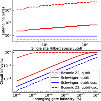
Figure 15: Advantage of hybrid qubit-oscillator hardware over qubit-only hardware, assuming simplistic qubit circuit construction. Entangling gate count as a function of single site Hilbert space cutoff (upper plot) and circuit fidelity as a function of entangling gate fidelity (lower plot) for the $(1+1)$D $\mathbb{Z}_{2}$-Higgs model (dotted lines) and $U(1)$ quantum link model (referred to as Schwinger model - solid lines) including gauge fields for qubit-only hardware (red) using the Fock binary encoding compared to hybrid qubit-oscillator hardware (blue) for one Trotter step for 2 matter sites. The qubit $\mathbb{Z}_{2}$-Higgs model requires square roots which are calculated with 2 Newton iterations. Gate counts are reported in the text; we count CNOT gates for all-qubit hardware and $\operatorname{C\Pi}$ for hybrid oscillator-qubit hardware (single qubit gates and beamsplitters are assumed to be ideal). We set the Hilbert space cutoff to be equal to the number of sites in the system. Trotter error is not taken into account in the circuit fidelity as it will be the same for circuits considered here.

In Fig. 15, we compare gate counts for the $U(1)$ quantum link model and $\mathbb{Z}_{2}$-Higgs model in both types of hardware. The jumps in the qubit-only lines are due to the logarithmic scaling of the qubit register required to represent increasing Hilbert space cutoffs. The $U(1)$ quantum link model in $(1+1)$D corresponds to the Schwinger model, for which we report the number of CNOT gates required for one Trotter step to be [122]:

$$N_{\mathrm{CNOT/U(1)}}=9n^{2}-7n+34.$$ (148)

In comparison, the number of entangling gates required to implement these models in hybrid qubit-oscillator hardware is $\mathcal{O}(1)$. The number of conditional parities $\operatorname{C\Pi}$ required for the $\mathbb{Z}_{2}$-Higgs model and $U(1)$ quantum link model is:

$$N_{\mathrm{C\Pi/\mathbb{Z}_{2}}} =2$$ (149)

$$N_{\mathrm{C\Pi/U(1)}} =8.$$ (150)

	Qubit (Fock-binary)	Qubit-oscillator
$\mathbb{Z}_{2}$-Higgs model	$\mathcal{O}(\log_{2}(N_{\mathrm{max}})^{2})$	$\mathcal{O}(1)$
Schwinger model	$\mathcal{O}(\log_{2}(S)^{2})$ [122]	$\mathcal{O}(1)$

Table 7: Asymptotic scaling of the number of entangling gates with Hilbert space cutoff for one Trotter step in qubit-only and hybrid qubit-oscillator hardware in $(1+1)$D for the $\mathbb{Z}_{2}$-Higgs model with bosonic matter and the $U(1)$ quantum link model (referred to as the Schwinger model), keeping the gauge fields. $N_{\mathrm{max}}$ is the maximum Fock state at each bosonic matter lattice site. $S$ is the spin length leading to a Hilbert space cutoff of $2S+1$. The decay time of the bosonic modes increases linearly with Fock state in hardware.

Finally, we consider the corresponding circuit fidelities for the execution of one Trotter step for a system size of 2 sites. This is of utmost importance in the NISQ era where entangling gate fidelities rarely reach above $99.99\%$ [115]. In the fidelity calculation, we assume single qubit gates and beamsplitters to have ideal fidelity. We plot the circuit fidelity with regards to the entangling gate fidelity which corresponds in the all-qubit case to the CNOT gate fidelity and in the hybrid oscillator-qubit case to the $\operatorname{C\Pi}$ fidelity. Both types of hardware are based on the same oscillator-qubit circuits and will therefore encounter the same Trotter error (the bosonic $\mathbb{Z}_{2}$-Higgs model mapping is exact). Therefore, Trotter error is not taken into account in the circuit fidelity.

In the fault-tolerant era, ideal fidelities can only be approached with large distance codes which directly increase the space-time volume of the computation. Therefore, even in the fault-tolerant era for all-qubit hardware, entangling gate fidelities will be of concern, and non-error corrected hybrid oscillator-qubit hardware may provide advantages. This is especially true considering the extremely large circuit depths required when mapping gauge fields or bosonic modes to qubits. In the case of the $\mathbb{Z}_{2}$-Higgs model which contains bosonic matter, the square root factors lead to the requirement for extremely high fidelity operation of a qubit-only device, unless we see substantial algorithmic improvements in arithmetic. In this case, the experimental improvements in hybrid oscillator-qubit hardware may enable progress to be made on bosonic models even in relatively large system sizes such as the ones presented here. Conversely, however, we must note that the harmonic approximations used for native bosonic hardware may break down if large occupation cutoffs are required. For these reasons, this work suggests the existence of a regime of advantage but experimental and algorithmic realities need to be considered in greater detail to verify this advantage.

These results suggest that for Trotter-based simulations an advantage may be seen for hybrid hardware; however, a full comparison of qubit to oscillator-qubit devices is challenging to make. For one, a full comparison between the two requires that we compare the best implementations of the best algorithms for both hardware in an agnostic fashion. This is especially significant because alternative methods of simulation, such as qubitization or LCU [129, 130] do not require square roots at the price of an increased number of ancillary qubits. A full comparison would need to consider optimized versions of all available algorithms for both hardware platforms. Second, a more detailed discussion of the approximation errors incurred in the approaches (such as the large $S$ limit or the use of BCH approximations and the different errors in the Trotter formula based on the form of the Hamiltonian) is needed to properly compare different approaches. For these reasons, we cannot claim that this work suggests a universal advantage for simulating $\mathbb{Z}_{2}$ or $U(1)$ LGTs, but it does strongly suggest advantages are likely to exist in certain regimes and subsequent work is needed to understand the shape and size of these regions of advantage.

VI Measurements, algorithms and numerical benchmarks

In the previous sections, we have introduced all of the necessary compilation methods to simulate both the $\mathbb{Z}_{2}$-Higgs model and $U(1)$ quantum link model (with either bosonic or fermionic matter) in $(2+1)$D. As an explicit demonstration of these compilation methods in practice, in this Section we apply them to the $(1+1)$D variants of these two models. In particular, we present schemes to measure short- and long-range observables, and near-term (Trotter and variational approaches) and longer-term (quantum signal processing) algorithms for dynamics and ground-state preparation, which we benchmark numerically. In particular, to enable approximate ground state preparation using the variational quantum eigensolver (VQE) approach, we show how to measure the expectation value of the Hamiltonian. We also develop an ancilla-free method for using post-selection on the Gauss’s law gauge constraint for partial error detection.

We use Bosonic Qiskit for our simulations [60]. Each mode is represented with $\lceil\log_{2}(N_{b}+1)+1\rceil$ qubits, with $N_{b}$ is the total number of bosons in the system (which is conserved for our Hamiltonians) in order to make sure that the commutation relation for the truncated mode operators obeys $[a,a^{\dagger}]=1$ within the accessible Hilbert space. We also include single qubit amplitude and phase damping error channels using Qiskit Aer [131] and neglect photon loss and dephasing of the cavities. For transmon qubits, $T_{2}\sim T_{1}$ [85]. In tantalum transmons it was shown that $T_{1}>500$ $\mu$s is possible [85]; however, we choose a conservative value of $T_{1}=T_{2}=200$ $\mu$s [84]. This implies a pure dephasing time of $T_{\phi}=(\frac{1}{T_{2}}-\frac{1}{2T_{1}})^{-1}=400$ $\mu s$. Cavities have very little dephasing and photon loss times exceeding $1$ms [77], and most of our numerical examples do not access high Fock states, justifying us neglecting these processes.

This section is structured as follows. In Sec. VI.1, we discuss the (1+1)D variants of the $\mathbb{Z}_{2}$-Higgs and $U(1)$ quantum link models, their physics and challenges in previous approaches to solve them. In Sec. VI.2 we investigate time dynamics, numerically benchmarking a simulation on the $\mathbb{Z}_{2}$-Higgs model while including the dominant source of noise. In Sec. VI.3, we show that ground states of these models can be prepared using a variational quantum eigensolver (VQE), for which we introduce an optimization technique better adapted to noise. In Sec. VI.4, we analyze in detail how to mitigate the influence of shot noise and decoherence. In Sec. VI.5, we show how to measure observables relevant to identifying phase-transitions, such as the pair-gap, the superfluid density, and the string order correlator with respect to the VQE ground states. In Sec. VI.6 we present a perspective on how to implement a ground-state preparation technique with provable success probabilities, known as quantum signal processing.

VI.1 Models and Physics

To begin, we present the two models that we use for explicit demonstration throughout this section: the $\mathbb{Z}_{2}$-Higgs model containing bosonic matter sites, and the $U(1)$ quantum link model containing fermionic matter sites, both in $(1+1)$D. These models are special cases of the more general LGT Hamiltonians presented in Section I.1; we discuss the details and implementation of each below. In particular, we can use the architectures presented in Fig. 2c),d) for one spatial dimension by winding a “snake” pattern through the square lattice. This way, every cavity and qubit represents either a gauge field or matter site.

VI.1.1 $\mathbb{Z}_{2}$-Higgs model 

The $\mathbb{Z}_{2}$ lattice gauge theory was introduced by Wegner [61] as a simple model showing signatures of confinement and deconfinement at the critical point [132], making it an ideal testbed for early testing of novel methods for LGT simulations. In two spatial dimensions in the absence of an electric field, its ground state encodes a spin-$1/2$ degree of freedom and can therefore be used for quantum error correction [133, 134]. $\mathbb{Z}_{2}$ lattice gauge theory with bosonic matter is reminiscent of the Higgs sector coupled to the non-Abelian $SU(2)$ electroweak gauge sector (W and Z bosons) of the $(3+1)\mathrm{D}$ Standard Model of particle physics with the two simplifications of a lower dimensionality and a $\mathbb{Z}_{2}$ gauge field instead of the non-Abelian $SU(2)$ electroweak gauge fields. The Hamiltonian in $(1+1)$D is written as follows:

$$\hat{H}_{\mathbb{Z}_{2}} =-g\sum_{i=1}^{L-1}\hat{X}_{i,i+1}+U\sum_{i=1}^{L}\hat{n}_{i}^{2}$$

$$\quad-J\sum_{i=1}^{L-1}\left(\hat{a}^{\dagger}_{i}\hat{Z}_{i,i+1}\hat{a}_{i+1}+\mathrm{h.c.}\right),$$ (151)

where the symbols are the same as described in the introduction (see Section I.1), and $L$ is the number of sites in the chain.

The $\mathbb{Z}_{2}$ model in $(1+1)$D in the hardcore boson limit $U\rightarrow\infty$ has previously been investigated in depth [135], revealing intriguing phase transitions between insulating and Luttinger liquid phases [136, 132]. A digital simulation of this model for hardcore-bosons has been performed in Ref. [38]. A basic building block of two matter and one gauge field site has been implemented in an experiment with ultracold atoms in a Floquet approach [23]. However, this approach is challenging to generalize away from the single particle limit in the presence of on-site interactions $U$ due to Floquet heating, which is important when considering parameter regimes away from the hardcore-boson limit. Our digital implementation enables a fully flexible study of this model, including regimes away from the hardcore limit. While we focus here on the implementation aspects of the model, enabling a study away from the hardcore boson limit, we study its physics and phase diagram in a separate publication [137].

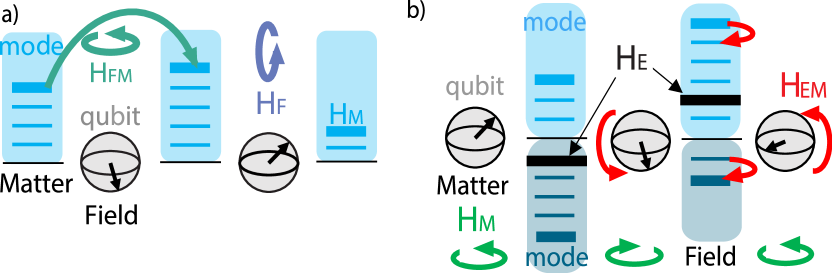
Figure 16: Illustration of the lattice gauge theories considered in section VI. a) $\mathbb{Z}_{2}$-Higgs model. Bosonic matter (blue) is represented by bosonic modes on the sites whereas a qubit represents the gauge field on the links (gray). The gauge-invariant coupling between the two (green) hops a boson from one site to a neighbouring site and phase flips the qubit on the link (by acting with $\hat{Z}$). The electric field term acts on the qubits with $\hat{X}$. $\hat{H}_{\mathrm{F}}$, $\hat{H}_{\mathrm{M}}$, $\hat{H}_{\mathrm{FM}}$ are the first, second and third terms in Eq. (151), respectively. b) $U(1)$ quantum link model. Matter sites are represented by qubits and the gauge fields on the links by a pair of bosonic modes realizing the Schwinger-boson encoding. An example for their occupation number is illustrated with a thick line, the occupation number increases towards the top/bottom for the top/bottom mode. The value of the electric field is the difference in occupation between the constituting field modes (black thick line). The gauge-invariant hopping (red) exchanges an excitation between two neighbouring qubits while incrementing or decrementing the gauge field (equivalent to transferring a boson from one of the composing modes to the other). A $\hat{Z}$ term on each matter qubit with opposite sign represents a staggered mass. $\hat{H}_{\mathrm{E}}$, $\hat{H}_{\mathrm{M}}$, $\hat{H}_{\mathrm{EM}}$ are the first, second and third terms in Eq. (152), respectively.

VI.1.2 $U(1)$ quantum link model 

The $U(1)$ quantum link model constrained to $(1+1)$D and fermionic matter  [64, 65, 66, 67, 68] reads

$$\hat{H}_{U(1)} =\frac{g^{2}}{2}\sum_{i=1}^{L-1}\left(\hat{S}^{z}_{i,i+1}+\frac{\tau}{2\pi}\right)^{2}+M\sum_{i=1}^{L}(-1)^{i}\hat{c}^{\dagger}_{i}\hat{c}_{i}$$

$$+\frac{\tilde{J}}{2S}\sum_{i=1}^{L-1}\left(\hat{c}^{\dagger}_{i}\hat{S}^{+}_{i,i+1}\hat{c}_{i+1}+\mathrm{h.c.}\right),$$ (152)

where compared to Eq. (3), the definition of $J$ differs by $\tilde{J}=J/2$ and we set $\sqrt{S(S+1)}\rightarrow S$ in the denominator of the hopping term, i.e. we consider the limit $S\rightarrow\infty$.

This model can be connected to a continuum field theory by introducing a lattice spacing $a$ by $J\rightarrow J/a$ and $g\rightarrow g\sqrt{a}$ and taking the limit $a\rightarrow 0$.

This model shares many properties with quantum chromodynamics in $(3+1)\mathrm{D}$: chiral symmetry breaking, confinement, a $U(1)_{A}$ quantum anomaly, and a topological $\tau$-term, which gives rise to a non-trivial topological vacuum structure [138, 70]. Due to the sign problem, this $\tau$-dependence of the model cannot be studied with quantum Monte Carlo methods. One possible way to circumvent the sign problem is using the tensor network (TN) approach, in particular matrix product states (MPS) in $(1+1)\mathrm{D}$. Using MPS, the spectrum of the $U(1)$ quantum link model has been computed, and the model has been studied at non-zero temperature, non-zero chemical potential, and with a non-zero $\tau$-term [71, 72, 73, 139, 140] (see Ref. [141] for a review). In particular, Refs. [71, 72] studied the first-order phase transition at $\tau=\pi$, in which the CP symmetry is spontaneously broken. The first-order phase transition line terminates at a second-order critical point [71, 72]. This model has been extensively simulated in superconducting qubits [33, 34, 35, 36, 37, 40, 142].

Despite these successes of studying sign-problem afflicted regimes with TN, TN approaches have several limitations. First, highly entangled states such as those with volume law entanglement can occur in the evolution after a quench or in thermal states, and cannot be efficiently described using matrix product states [143], the most widely used TN. This is particularly apparent in multi-stage thermalization dynamics such as after instabilities [144]. Second, the computational cost of TN algorithms increases with increasing dimensionality of the lattice field theory under consideration. For MPS, a particular kind of one-dimensional TN, the leading-order computational cost of the variational ground-state optimization in the case of open boundary conditions scales as $\mathcal{O}(D_{b}^{3})$ [145, 146, 147], where $D_{b}$, called the bond dimension, indicates the tensor size in the MPS. For the generalization to $(2+1)\mathrm{D}$, called projected entangled pair states (PEPS) [148], computational costs can scale up to $\mathcal{O}(D_{b}^{10})$ [149]. These costs are still polynomial in the bond dimension, but substantially limit the values of $D_{b}$ that can be reached in practice. There have been TN studies of gauge theories in $(2+1)\mathrm{D}$ and $(3+1)\mathrm{D}$ [150, 151, 152], but designing efficient TN algorithms in higher dimensions remains a fundamental challenge.

For this Hamiltonian (Eq. (152)), Refs. [153, 72] explored whether the gauge degrees of freedom can be efficiently represented with finite-dimensional systems. For intermediate values of the coupling, $g\sqrt{a}\sim 0.1$, Ref. [153] demonstrated that the results converge rapidly, implying that a reasonable accuracy can be obtained even with small cutoffs $N_{\mathrm{max}}$ of the gauge-field truncation. To be more precise, the truncated $U(1)$ quantum link model yielded a fast convergence to the exact ground state for $N_{\mathrm{max}}$ ranging from 3 to 9, reaching sub-permille precision in the energy density for $N_{\mathrm{max}}=9$ [153]. However, when approaching the continuum limit, $g\sqrt{a}\to 0$, the increasing electric field fluctuations require an increasingly large number of states and therefore an increasingly large (up to exponentially large) cutoff. This strongly motivates applying hybrid oscillator-qubit quantum devices to $U(1)$ lattice gauge theory.

VI.2 Dynamics

To illustrate the power of our digital approach to qubit-boson quantum simulation of lattice gauge theories we show that some gauge-constrain-induced dynamics can be observed in near-term noisy hardware. Here, we focus on the $\mathbb{Z}_{2}$-Higgs model for $U=0$.

We first need to prepare an initial state of interest. As discussed in the exposition of the cQED platform in Section I.2, it is straightforward to prepare the modes in a product state of Fock states. We consider a $L=5$-site chain prepared in the states $\ket{\psi_{0}}=\ket{00100}$ and $\ket{\psi_{1}}=\ket{00200}$. The limitation to five sites is not restrictive for short timescales – because the interactions are short-range, excitations spread with a finite velocity and as long as the “lightcone” does not reach the boundary, the results obtained here are the same as would be in a larger system. The qubits representing the $\mathbb{Z}_{2}$-Higgs model gauge fields must then be initialised according to Gauss’s law, which requires consistency between the qubits and the parity in each mode: choosing the leftmost gauge field qubit to be in $\ket{+}$ and the sites to be in Fock state $\ket{00100}$, the gauge field qubits situated on the links between the bosonic sites need to be initialized in $\ket{++--}$. Likewise, for bosonic sites in $\ket{00200}$, the corresponding gauge field state is $\ket{++++}$. The fact that the state of the gauge fields is fully determined by the state of the sites shows us that the gauge fields could be integrated out, which is usually the case for lattice gauge theories in $(1+1)$D. The reverse is not true however: the state of the gauge fields does not fully determine the state of the bosonic sites but only their parity. This is in contrast to hard-core bosons, where the parity fully determines the occupation number [132]. See also Ref. [154] for a more in-depth consideration of these dynamics in the context of hybrid simulation in trapped ions.

We evolve the initial states $\ket{\psi_{0}}$ and $\ket{\psi_{1}}$ under the $\mathbb{Z}_{2}$-Higgs model with $U=0$ using a first-order Trotterization $e^{-i\hat{H}_{\mathbb{Z}(2)}t}\approx(\hat{U}_{1}\hat{U}_{2})^{r}$ and timestep $\Delta t=t/r$ with

$$\hat{U}_{1} =\prod_{i}^{L}e^{-ig\hat{X}_{i,i+1}\Delta t},$$ (153)

$$\hat{U}_{2} =\prod_{i=1}^{L-1}e^{-iJ\hat{Z}_{i}\left(\hat{a}^{\dagger}_{i}\hat{a}_{i+1}+\hat{a}_{i}\hat{a}^{\dagger}_{i+1}\right)\Delta t}.$$ (154)

We have discussed in Section IV how the time evolution operator for the individual Hamiltonian terms in Eq. (151) can be implemented using native gates in our proposed architecture.

At the end of the simulation, we measure the state of the qubits and modes. The measurement of the mode occupations are carried out bit-by-bit in a binary representation, first mapping the boson number parity onto the qubit using an SQR gate, making a mid-circuit measurement, resetting the qubit, then measuring the super-parity and so on, as has been demonstrated experimentally [95, 96]. This requires a circuit with a depth that is logarithmic in the maximum boson occupation cutoff. If the qubits representing the gauge fields are read out first, they can be reused to iteratively read out the Fock state of the cavity mode to which they are dispersively coupled.

To show that these dynamics can be probed in near-term hardware, we implement the $(1+1)\mathrm{D}$ gate sequences in Bosonic Qiskit [60, 155], assuming an implementation in which the $\mathbb{Z}_{2}$ gauge fields are encoded in transmons.

In order to simulate the dynamics in presence of the noise, we need to specify the gate durations we assume for the potential experimental implementation using the hardware in Sec. I.2. We assume a value of $\chi\approx 3$ MHz for the dispersive interaction strength. The duration of each Trotter step is then dominated by the conditional beamsplitter operation, which is on the order of $2.1$ $\mu$s, consisting of two conditional parity gates which take $1$ $\mu$s each and one beamsplitter which has a duration on the order of $100$ ns [103, 86]. Single qubit gates take on the order of $10$ ns. The Trotter step size in our numerical simulation, $\Delta t=0.1/J$, was chosen to be small enough to recover the expected physical behavior in comparison to exact diagonalisation. We chose $1000$ shots per circuit, which leads to both low shot-noise errors as well as a realistic experimental runtime: because each Trotter step has depth $2$, a depth one circuit takes $<2.2\mu$s and we need $85$ Trotter steps to evolve to $Jt=8.5$. Each circuit therefore takes at most $2\times 85\times 2.2\mu\mathrm{s}=374\mu$s. We measure $85$ circuits and therefore, $1000$ shots per circuit leads to a total projected time to take the experimental data of Fig. 17b) for $g=5J$ of $1000\times 85\times 374\mu\mathrm{s}\approx 32$s.

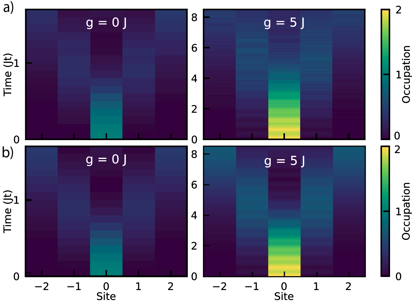
Figure 17: Trotterized dynamics in the $\mathbb{Z}_{2}$ model in the presence of transmon decoherence. Left: Free hopping regime $U/J=g/J=0$. Initial bosonic state $\ket{00100}$. Right: Large field regime $U=0$, $g/J=5$. Initial bosonic state $\ket{00200}$. a) Numerically simulated using Bosonic Qiskit, $1000$ shots chosen to reduce shot-noise errors to a few percent, first-order Trotterization, Trotter step $0.1/J$. b) Exact diagonalisation results.

On the one hand, in the regime of infinite hopping strength (i.e., $g=0$), starting from the Fock state $\ket{00100}$ with open boundary conditions, we find a linear light-cone-like spreading of the boson, c.f. Fig. 17. On the other hand, large field strengths prohibit the gauge fields from flipping during hopping events which leads the boson to remain confined to the central site, as predicted and observed in Ref. [135, 23, 38] in cold atoms. Strikingly, for large field strengths, when starting from the Fock state with an even initial number of bosons such as $\ket{00200}$, we again find a linear light-cone even in the large field strength regime. We find that the hopping takes place on a much slower time scale. This hopping is enabled by a perturbative energy-conserving pair-hopping process of strength $J^{2}/2g$ in which a qubit which is flipped by a first boson hopping and then flipped back to its original value by the second boson hopping [137]. Despite the transmon decoherence and the much longer time scale (the circuit to evolve to the latest time point for $g=5J$ takes around $2\times 85\times 2.2\mu\mathrm{s}\approx 374\mu$s experimental time), these coherent dynamics are observable and match exact diagonalisation.

VI.3 Qubit-boson ground state preparation with VQE

In this section, we show how the variational quantum eigensolver algorithm (VQE) [156, 157] (see Refs. [158, 159, 160, 161] for important follow-up works) can be implemented not only on oscillators/modes [162, 163, 164], but also on our proposed hybrid qubit-oscillator architecture to prepare ground states of the $\mathbb{Z}_{2}$-Higgs and U$(1)$ quantum link model. VQE is a variational ansatz for the ground state wavefunction in which layers of unitaries $\hat{U}_{k}$ act on some initial state. The unitaries in our approach, sometimes called the quantum approximate optimisation algorithm, are related to the Hamiltonian

$$\hat{H}=\sum_{k,i}\hat{h}_{k}(i),$$ (155)

where $\hat{h}_{k}(i)$ are terms of the Hamiltonian with $i$ the site index on which they are applied. We choose

$$U_{k}(\theta,i)=e^{i\theta\hat{h}_{k}(i)},$$ (156)

where $\theta$ is a variational parameter which is optimized. Each gate in the ansatz has an independent angle; we denote the vector of angles with $\boldsymbol{\theta}$.

In the VQE, the classical and quantum processors work together to reach the ground state by executing an optimization algorithm which updates the vector of ansatz angles $\boldsymbol{\theta}\rightarrow\boldsymbol{\theta}^{\prime}$, and uses the quantum computer to measure the expected energy of the anstatz characterised by those angles $\braket{\psi(\boldsymbol{\theta}^{\prime})}{\hat{H}}{\psi(\boldsymbol{\theta}^{\prime})}$. The intuition behind this VQE procedure comes from the fact that for our choice of ansatz, a sufficiently large number of layers and a particular choice of $\boldsymbol{\theta}$, VQE realizes adiabatic state preparation (note the parallel between choosing the gate variable angles to be proportional to time for dynamics, and choosing them to be the optimisation parameter for ground state search). Therefore we know that in principle, VQE is able to prepare the ground state if the Hamiltonian has a large enough gap such that the necessary evolution time is within the coherence time of the quantum computer. In the absence of first-order phase transitions, the gap is always polynomial in the system size and hence an efficient state preparation path can be found. In the gauge theory setting, constructing a variational ansatz this way also has the advantage of fulfilling Gauss’s law. This is exactly the case if every term in the Hamiltonian conserves Gauss’s law individually (which will be the case for us below). If this is not true, Gauss’s law can be fulfilled approximately by choosing the angles small enough to essentially realize the Trotter limit of adiabatic time evolution.

The hope behind VQE is that by minimizing the energy with respect to the $\boldsymbol{\theta}$ angles, a circuit could be found which prepares the ground state in a shallower circuit than would be required for adiabatic state preparation, which in this digital setting would require Trotterisation. In the following, we discuss VQE in the cQED architecture for the $\mathbb{Z}_{2}$-Higgs model and $U(1)$ quantum link model in $(1+1)$D.

VI.3.1 $\mathbb{Z}_{2}$-Higgs model 

In the case of the $\mathbb{Z}_{2}$-Higgs model, the $\hat{U}_{k}$ required for the ansatz discussed in the first paragraph of (Sec. VI.3), Eq. (156), are

$$\hat{U}_{1}(\theta,i) =e^{-\theta\hat{Z}_{i,i+1}(\hat{a}^{\dagger}_{i}\hat{a}_{i+1}-\hat{a}_{i}\hat{a}^{\dagger}_{i+1})}$$ (157)

$$\hat{U}_{2}(\theta,i) =e^{i\theta\hat{Z}_{i,i+1}(\hat{a}^{\dagger}_{i}\hat{a}_{i+1}+\hat{a}_{i}\hat{a}^{\dagger}_{i+1})}$$ (158)

$$\hat{U}_{3}(\theta,i) =e^{-i\theta\hat{X}_{i,i+1}}$$ (159)

$$\hat{U}_{4}(\theta,i) =e^{-i\theta\hat{n}_{i}^{2}}.$$ (160)

While technically not necessary (all other gates together are already able to prepare the ground state by approximating an adiabatic evolution), we find that including $\hat{U}_{1}$ leads to a lower energy error for the same number of layers than when it is not included. All of the above unitaries can be realized with our native gate set using techniques previously discussed; in particular $\hat{U}_{1}$ and $\hat{U}_{2}$ are conditional beamsplitters (see Eq. (19)), $\hat{U}_{3}$ is a single-qubit rotation, and $\hat{U}_{4}$ can be implemented using a SNAP gate (see Section III.1.3, or alternatively App. B for an ancilla-free implementation).

Using these resource unitaries, we construct an $M$-layer ansatz with $N$ field sites and $N+1$ matter sites as

$$\ket{\psi_{M}(\boldsymbol{\theta})}=\prod_{l=1}^{M} \bigg{[}\prod_{i=1}^{N}\hat{U}_{3}(\gamma^{i}_{l},i)\prod_{i=1}^{N+1}\hat{U}_{4}(\delta^{i}_{l},i)\vphantom{\int_{1}^{2}}$$

$$\quad\prod_{i\in\text{even}}^{N}\hat{U}_{2}(\alpha^{i}_{l},i)\hat{U}_{1}(\beta^{i}_{l},i)$$

$$\quad\prod_{i\in\text{odd}}^{N}\hat{U}_{2}(\alpha^{i}_{l},i)\hat{U}_{1}(\beta^{i}_{l},i)\bigg{]}\ket{\phi},$$ (161)

where $\ket{\phi}$ is an easily-preparable state, $\boldsymbol{\theta}$ is a vector of the $(4N+1)M$ real-numbered angles in this ansatz, and the products over $i\in\text{even (odd)}$ include only the field qubits with even (odd) index. This means that every single gate in each layer and at each site has a different angle to be optimised. Fig. 18a) shows one layer of the VQE ansatz.

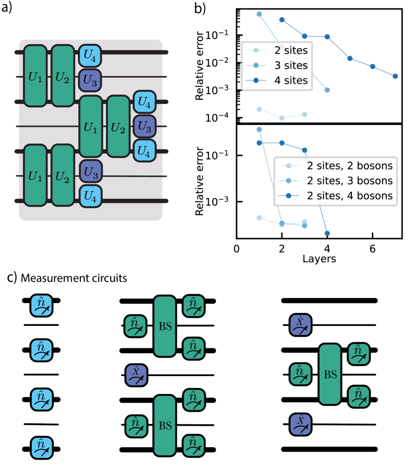
Figure 18: VQE for the $\mathbb{Z}_{2}$-Higgs model in $(1+1)$D. a) A single layer of the VQE ansatz. The different colors refer to the different Hamiltonian terms. b) Numerical simulation of the VQE without shot noise and decoherence for $U/J=g/J=1$. We show the relative error $|E_{\mathrm{VQE}}-E_{0}|$/$|E_{0}|$ between the estimated ground state energy $E_{\mathrm{VQE}}$ obtained via VQE and the true ground state energy $E_{0}$ as a function of the number of layers for varying number of sites at unit filling (top), and varying numbers of bosons for two sites (bottom). Fluctuations in performance between runs of the VQE (caused by the stochastic optimizer) are small, leading to fluctuations of the relative error of at most a factor of $5$, c.f. the deviation of the $4$-site results from a smooth line; we show the result of a typical single run. c) The three sets of measurement circuits we use for measuring the energy: gauge-invariant hopping (green), the electric field terms (purple), and the onsite interaction at each site (blue). The colors in panel c) correspond to the ones in a). We note that qubit measurement corresponds to a measurement of $\hat{Z}$, while for modes corresponds to measurement of $\hat{n}$.

Since the $\mathbb{Z}_{2}$ resource unitaries in Eq. (157 - 160) exactly preserve Gauss’s law (in the absence of decoherence), the entire circuit evolution will take place within the Gauss’s law subspace chosen by the initial state. Restricting the evolution of VQE circuits within a particular subspace is a powerful technique introduced in prior work [165], with many applications to constrained optimization problems such as maximum independent set [166]. Here, we choose the initial state $\ket{\phi}$ to be a simple-to-prepare state which obeys Gauss’s law, specifically, a product state of Fock states with unit occupation.

Because we aim to provide scalable methods adapted for large system sizes, global optimizers such as ‘DIRECT’ which were used in previous studies of lattice gauge theories [28] are not well suited here. We compared optimizers (with Python Scipy names ‘COBYLA’, ‘Nelder-Mead’, ‘CG’, ‘trust-constr’, ‘BFGS’, ‘L-BFGS-B’, ‘SLSQP’) and find that, among the optimizers which were tested, ‘SLSQP’ (Sequential Least Squares Programming) has the fastest convergence rates for the $\mathbb{Z}_{2}$ model without qubit decoherence or shot noise, measuring the energy by calculating the expectation value of the Hamiltonian matrix directly with the circuit state vector without shot noise.

We find that the VQE circuit (without noise and therefore no sampling error) can estimate ground state energy with relative error with respect to the true ground state energy of around $10^{-3}$ for two, three, and four sites using one, four, and seven layers, respectively, as can be seen in Fig. 18b. The VQE requires on average around $10^{2}$, $10^{3}$, and $10^{4}$ circuit evaluations for two, three, and four sites respectively, an increase which is due to the commensurate increase in the number of Fock states required to represent a larger Hilbert space for unit filling. Increasing the number of layers increases the total number of variational parameters, which can lead to a higher final fidelity; however, this presents a tradeoff – in the presence of noise, reliable results can be extracted only from shallow depth circuits. Thus, the overall fidelity will decrease when a large number of layers is used [167].

Furthermore, we find that the higher the boson filling, the larger the number of layers required, with up to four layers required for four bosons in two sites to reach a relative error below $10^{-3}$. This may be related to the increased size of the Hilbert space, i.e., due to the increase in possible combinations for distributing the bosons among a set number of sites.

To measure the expectation value of the Hamiltonian as required for the VQE optimisation procedure, we discuss how to measure each term of the Hamiltonian individually [158]. The field term $\braket{-g\sum_{i=1}^{L-1}\hat{X}_{i,i+1}}$ is a simple sum of $X$-basis qubit measurements. The onsite interaction term on a single site $i$ can be measured by reading out the photon number of the cavity using the binary search readout [95, 96]. This enables the single-shot readout of $\hat{n}_{i}$, which can then be used to reconstruct $\langle n_{i}^{2}\rangle$. For the gauge-invariant hopping term $-J\sum_{i=1}^{L-1}\braket{\hat{Z}_{i,i+1}\left(\hat{a}^{\dagger}_{i}\hat{a}_{i+1}+\mathrm{h.c.}\right)}$, we are faced with the difficulty that we can not directly read out the beamsplitter term by measuring the cavities in the number basis. Instead, we note the following identity:

$$\bra{\psi}\hat{a}_{i}^{\dagger}\hat{a}_{i+1}+\mathrm{h.c.}\ket{\psi}$$

$$=\bra{\tilde{\psi}}\text{BS}_{i,i+1}\left(\frac{\pi}{2},\frac{\pi}{4}\right)(\hat{a}_{i}^{\dagger}\hat{a}_{i+1}+\mathrm{h.c.})\text{BS}_{i,i+1}^{\dagger}\left(\frac{\pi}{2},\frac{\pi}{4}\right)\ket{\tilde{\psi}}$$

$$=\bra{\tilde{\psi}}\left(\hat{a}_{i}^{\dagger}\hat{a}_{i}-\hat{a}_{i+1}^{\dagger}\hat{a}_{i+1}\right)\ket{\tilde{\psi}}$$

$$=\bra{\tilde{\psi}}\hat{n}_{i}\ket{\tilde{\psi}}-\bra{\tilde{\psi}}\hat{n}_{i+1}\ket{\tilde{\psi}},$$ (162)

where we have inserted $\mathds{1}=\text{BS}_{i,i+1}\left(\frac{\pi}{2},-\frac{\pi}{4}\right)\text{BS}_{i,i+1}\left(\frac{\pi}{2},\frac{\pi}{4}\right)$ on either side of the hopping, and have cast the expression in terms of the transformed state $\ket{\tilde{\psi}}=\text{BS}_{i,i+1}(\frac{\pi}{2},\frac{\pi}{4})\ket{\psi}$. Thus, much like a Hadamard gate facilitates an $X$-basis measurement for qubits, we can measure the expectation value of a bosonic hopping term by ‘rotating’ the modes into the Fock state basis via a 50:50 beamsplitter, followed by a Fock-basis measurement. By correlating the result with that of the gauge field link $Z$-basis measurement result, one can reconstruct the expectation value of the gauge-invariant hopping.

Only commuting terms can be measured simultaneously; for the $\mathbb{Z}_{2}$ model, we therefore perform three separate measurement circuits to estimate the energy. In the first circuit in Fig. 18c, the onsite interaction is measured on all sites simultaneously. In the same circuit, it is possible to measure the field terms, though this step must precede measurement of the onsite interaction such that the gauge link qubits can then be reset and used for binary readout. Next, we measure half of the gauge-invariant hopping terms, preceeded by a measurement of the electric field ($\hat{X}_{i}$) at every other gauge link. Finally, the other half of the gauge-invariant hopping terms are measured along with the other half of the field sites.

In summary, in this section we showed that a VQE ansatz for the $\mathbb{Z}_{2}$-Higgs model which is specifically tailored to the types of operations available in hybrid qubit-oscillator hardware indeed only requires very few layers to determine the ground state for the small system sizes we can access numerically for proof of principle demonstrations. The implementation of this ansatz directly follows from the methods presented in the first part of this paper (Secs. II - IV), which implies that the hybrid qubit-oscillator hardware will require shallower circuits than qubit hardware as discussed in Sec. V.5. However, more work needs to be done beyond these proof of principle results to determine the circuit depths and the number of shots which will be required as a function of system size.

VI.3.2 $U(1)$ quantum link model 

In the following, we describe how to carry out a hybrid oscillator-qubit VQE of the $U(1)$ quantum link model in Eq. (152) in $(1+1)$D. Furthermore, we demonstrate how to detect the first-order phase transition at $\tau=\pi$ in our proposed architecture. While the correspondence between the model in Eq. (152) and quantum electrodynamics in $(1+1)$D is only applicable for an even number of lattice sites due to the staggering of the fermions, we also study an odd number of sites here for benchmarking purposes.

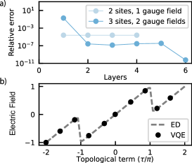
Figure 19: Numerical VQE results for the $U(1)$ quantum link model in $(1+1)\mathrm{D}$. We neglect shot noise and decoherence. a) Relative error between the estimated ground state energy obtained via simulated the VQE using Bosonic Qiskit [60] and the true ground state energy VQE results obtained for 2 and 3 sites. b) VQE compared to exact diagonalisation results. in The 1st order phase transition can be seen at $\tau=\pm\pi$ in the expectation value of the electric field $\frac{1}{2}\sum_{i=1}^{2}\braket{\hat{S}^{z}_{i,i+1}}=\frac{1}{2}\sum_{i=1}^{2}(\braket{\hat{n}^{a}_{i,i+1}}-\braket{\hat{n}^{b}_{i,i+1}})/2$ in the $(1+1)\mathrm{D}$ $U(1)$ quantum link model for a three site system and $4$ layers. Spin length chosen as $S=1$. $m/J=1,g/J=10$.

Following the same scheme as for the $\mathbb{Z}_{2}$-Higgs model, we choose resource unitaries that are generated by the individual terms of the Hamiltonian in Eq. (152). Furthermore, we leverage the Schwinger-boson mapping of the gauge fields as described in Sec. I.1, and map the fermions to qubits using the Jordan-Wigner encoding (which is particularly simple in $(1+1)$D). With these choices, we construct our VQE ansatz using the following resource unitaries:

$$\hat{U}_{S1}(\theta,i) =e^{i\theta\hat{Z}_{i}}$$ (163)

$$\hat{U}_{S2}(\theta,i) =e^{-i\theta(\hat{n}_{i,i+1}^{a}-\hat{n}^{b}_{i,i+1})}$$ (164)

$$\hat{U}_{S3}(\theta,i) =e^{-i\theta\left((n_{i,i+1}^{a})^{2}+(n_{i,i+1}^{b})^{2}\right)}$$ (165)

$$\hat{U}_{S4}(\theta,i) =e^{-i\theta\left(\hat{\sigma}^{+}_{i+1}\hat{a}^{\dagger}_{i,i+1}\hat{b}_{i,i+1}\hat{\sigma}^{-}_{i}+\mathrm{h.c.}\right)}$$ (166)

$$\hat{U}_{S5}(\theta,i) =e^{-\theta\left(\hat{\sigma}^{+}_{i+1}\hat{a}^{\dagger}_{i,i+1}\hat{b}_{i,i+1}\hat{\sigma}^{-}_{i}-\mathrm{h.c.}\right)}.$$ (167)

Each of these unitaries can be implemented using techniques described in prior sections. In particular, $\hat{U}_{S1}$ and $\hat{U}_{S2}$ are native gates – see Table 1. As explained in Sec. III.1.3, $\hat{U}_{S3}$ can be synthesized using a SNAP gate. Finally, the gauge-invariant hopping unitaries $\hat{U}_{S4}$ and $\hat{U}_{S5}$ can be implemented with the strategies described in Section IV.5.2.

Our ansatz for the wavefunction is

$$\ket{\psi_{M}(\boldsymbol{\theta})}=\prod_{l=1}^{M} \bigg{[}\prod_{i\in\text{even}}^{N}\hat{U}_{S5}(\alpha_{l},i)\hat{U}_{S4}(\beta_{l},i)$$

$$\;\;\;\prod_{i\in\text{odd}}^{N}\hat{U}_{S5}(\alpha_{l},i)\hat{U}_{S4}(\beta_{l},i)$$

$$\quad\prod_{i=1}^{N}\hat{U}_{S3}(\gamma_{l},i)\quad\prod_{i=1}^{N}\hat{U}_{S2}(\gamma_{l},i)$$

$$\prod_{i=1}^{N+1}\hat{U}_{S1}(\delta_{l},i)\vphantom{\int_{1}^{2}}\bigg{]}\ket{\phi},$$ (168)

for $N+1$ matter sites. Note that contrary to the ansatz for the $\mathbb{Z}_{2}$-Higgs model, each site has the same parameter such that there are only $4M$ total parameters.

The expectation value of the Hamiltonian, can be measured using correlated measurements. To evaluate the gauge-invariant hopping term, we first use $\hat{\sigma}^{+}=\frac{1}{2}(\hat{X}+i\hat{Y})$, to split it into

$$\hat{\sigma}^{+}_{i+1}\hat{a}^{\dagger}_{i,i+1}\hat{b}_{i,i+1}\hat{\sigma}^{-}_{i} +\mathrm{h.c.}$$

$$=\frac{1}{4}\bigg{(} \hat{X}_{i+1}(\hat{a}^{\dagger}_{i,i+1}\hat{b}_{i,i+1}+\mathrm{h.c.})\hat{X}_{i}$$

$$+ \hat{Y}_{i+1}(\hat{a}^{\dagger}_{i,i+1}\hat{b}_{i,i+1}+\mathrm{h.c.})\hat{Y}_{i}$$

$$+ \hat{X}_{i+1}(-i\hat{a}^{\dagger}_{i,i+1}\hat{b}_{i,i+1}+\mathrm{h.c.})\hat{Y}_{i}$$

$$+ \hat{Y}_{i+1}(i\hat{a}^{\dagger}_{i,i+1}\hat{b}_{i,i+1}+\mathrm{h.c.})\hat{X}_{i}\bigg{)}$$ (169)

Using our method in Eq. (162) we can map a measurement of the bosonic terms in above equation to a measurement of the number densities of the two modes. Correlating those number densities with the appropriate qubit measurements, we can therefore measure all four terms in the above expansion. Because we require two circuits to measure all possible lattice sites $i$, we require eight separate measurement circuits for the gauge-invariant hopping. All the other terms are straightforwardly accessible by measuring the values of the boson numbers in the modes [168, 95] and the state of the qubits.

Using Bosonic Qiskit [60], we implement this ansatz and test the convergence of the VQE with respect to the number of layers for $S=1$ and show the results in Fig. 19. For a single gauge field site and two matter sites, we initialize the system in the “vacuum state” $\ket{\downarrow 0\uparrow}$, where the middle label indicates the eigenstate of $S^{z}$, and assume perfect energy measurements, i.e. no shot noise and decoherence. We find that one layer is sufficient for obtaining a relative energy error of $10^{-5}$. This is related to the fact that the ground state for this system is given by $\frac{1}{\sqrt{2}}\left(\ket{\uparrow 1\downarrow}+\ket{\downarrow 0\uparrow}\right)$. Three sites, initialised in $\ket{\downarrow 0\uparrow 0\downarrow}$, we find from our numerical evaluations that two layers are required to attain low relative errors of $10^{-8}$, with only a small increase in total number of iterations from the two-site case.

In the regime of large $g$, the $U(1)$ quantum link model features a first order phase transition [138, 70] at half-integer values of $\tau/2\pi$. This can be seen trivially by taking $g\to\infty$, in which case the electric term dominates the Hamiltonian, pinning $\hat{S}^{z}$ at the integer closest to $\tau/2\pi$. This phase persists for finite $g$ until the mass reaches $M/g\approx 1/3$ (see definitions of $M$ and $g$ in Hamiltonian in Eq. (152)). The energy gap between the ground and first excited state is generally exponentially small in system size at first order phase transitions. Therefore, we expect that this transition will be relatively sharp and visible even for small systems of two or three sites. Hence, this is a good proof-of-principle target for small-scale experiments.

For various values of $\tau$ used to find ground states with the VQE ansatz discussed above (Eq. (163)-167), we measure the expectation value of the electric field (in the Schwinger-boson representation) $\braket{S^{z}_{i,i+1}}=\frac{1}{2}\braket{\hat{n}^{a}_{i,i+1}-\hat{n}^{b}_{i,i+1}}$. In Fig. 19 we indeed find sharp drops corresponding to the first order phase transition at $\tau=\pm\pi$. The Bosonic Qiskit VQE results match our exact diagonalization results to relative errors of around $10^{-7}$.

Our results show that our VQE approach using hybrid oscillator-qubit hardware can prepare ground states of the $U(1)$ quantum link model in $(1+1)\mathrm{D}$ for two and three site systems. Although in $(1+1)\mathrm{D}$ the $U(1)$ quantum link model can be probed with qubit-only hardware by integrating out the gauge fields, this would not generalize to higher dimensions. In that case, each gauge field link would be encoded in many qubits and Hamiltonian operations would be highly costly as discussed in Section  V.5. Another possible advantage of our approach is the usage of the Schwinger-boson constraint $\hat{n}_{a}+\hat{n}_{b}=2S$ as a (single) photon loss error detection scheme. This can be implemented by measuring the joint-parity of modes $a$ and $b$; to what extent this improves results from noisy hardware is an interesting direction for future exploration.

VI.4 VQE with hardware and shot noise

Next, we test the resilience of our methods to decoherence and shot noise in the energy measurements. To do so, we simulate the full measurement schemes that would be employed in the experiment and also include qubit decay and dephasing, which are the leading decoherence mechanism [169] for the small system sizes and unit filling we consider here (i.e., we neglect photon loss). For systems where large photon numbers are possible, mode decay will become appreciable. The model studied in this section is the $\mathbb{Z}_{2}$-Higgs model, for which we defined the ansatz in Sec. VI.3.1. We choose $U/J=g/J=1$, which we expect to be among the most difficult regimes to simulate due to the balanced competition between all energy terms. We consider three matter sites and two gauge links at unit filling, requiring three modes and two qubits.

We start by explaining how to measure the expectation value of the Hamiltonian in experiment. Following this, we first benchmark the simultaneous perturbation stochastic approximation (SPSA) optimiser [170, 171] optimizer (as opposed to SLSQP used so far) without shot-noise, as this is the optimizer of choice for optimisations with shot noise. We investigate how to use averaging over previous iterations to improve convergence of SPSA (still without any noise). Third, we run our improved optimisation procedure with shot noise. Upon finding that there is a certain independence to the number of shots in the initial stages of optimisation where the gradients are large, we further adapt our procedure to incrementally increase the number of shots during the optimisation. Fourth, we include hardware noise (qubit $T_{1}$ decay and additional pure $T_{\phi}$ dephasing) into the numerical simulation. Finally, we error-mitigate our results by implementing a procedure to post-select on preservation of Gauss’s law.

VI.4.1 Introducing shot noise in the energy measurement

We simulate a binary search routine [95, 96] for measuring the cavity in the Fock basis. This naively requires an additional readout qubit per cavity for the measurement (i.e. separate from the transmon qubits that encode the gauge field links). However, for the $\mathbb{Z}_{2}$-Higgs model we can remove this requirement by first measuring the gauge field links, and then reusing the qubits as ancillas for mode readout, c.f. Figs 18c. To do so, we measure and reset the field qubits prior to the cavity measurement. In our VQE simulations, we simulate the full binary search, which enables us to simulate the effective shot noise on the mode measurement that results from the qubit measurements. Due to shot noise, each experiment requires $\mathcal{O}(\frac{1}{\epsilon^{2}})$ circuit executions to estimate $\braket{\hat{H}_{\mathbb{Z}(2)}}$ to additive precision $\epsilon$.

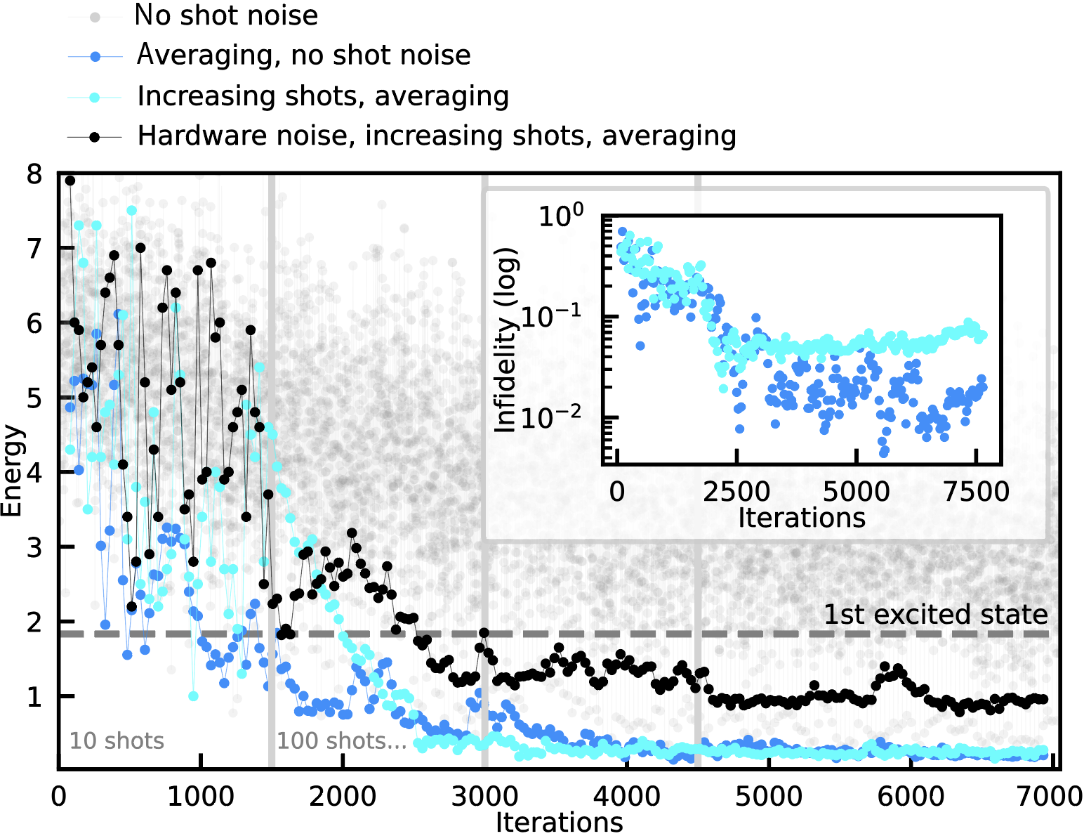
Figure 20: Numerical VQE results for the $\mathbb{Z}_{2}$-Higgs model including qubit decay and shot noise. $U/J=g/J=1$. Exact ground state energy is $E/J=0.02$. Energy is plotted in units of $J$. Three bosonic sites and two gauge fields, four layers in the ansatz, optimisation using SPSA. For the data without shot noise (gray dots), all iterations are plotted. For the rest of the data, only the iterations with averaged parameters are plotted. When averaging but without including shot noise (dark blue dots), we average the input variable parameters every 15 iterations, averaging over the input variable parameters found in the previous 7 iterations. For the light blue data, we include shot noise, increasing the number of shots after every 1500 iterations as indicated by the gray vertical lines. Black dots indicate the same procedure as the light blue data, but with hardware noise, i.e. qubit decay and dephasing. (Inset) Fidelity with the ground state as a function of the iteration number. Colors match the ones in the main panel.

VI.4.2 Using averaging in the stochastic VQE optimisation

In the presence of shot noise error, VQE optimisation is far more challenging [167, 161]. We use the SPSA, which is particularly well suited for VQE because it only evaluates the Hamiltonian twice per iteration regardless of the dimension of the optimization problem.

In Fig. 20 we show the energy found in each iteration using the SPSA optimiser. The gray dots indicate an optimisation without any shot noise, and we see that it does not converge within $7000$ iterations.

It has been found that averaging variable parameters can increase the performance of stochastic optimisation [172, 173]. We found in our case that the convergence of the SPSA optimiser, which is stochastic, can be improved by periodically choosing parameters for the next iteration which are averages of previous iterations. Therefore, we adapt our implementation of the SPSA optimiser in order to perform a parameter averaging step throughout the optimization: every $n$ iterations, we use the average of the variable parameters of the last $m$ iterations. It is important to not choose $n$ so small that the averaging is too frequent, resulting in a small sample size, or choose $m$ too large such that $m\gtrsim n$, which may constrain the optimisation too much and lead to trapping in local minima. In Fig. 20, we show data corresponding to $n=15$ and $m=7$ in dark blue. We find notable improvements using this strategy over the one without averaging, i.e. $n=1$ and $m=1$.

VI.4.3 Adaptive shot budget in the VQE optimisation

We now include shot noise in the estimation of the energy. The number of shots required for good convergence of the VQE is determined by the size of the energy gradient. Generally, gradients are larger in the first iterations and gradually decrease as the minimum is approached. This is evident in the large fluctuation between iterations for the early iterations $<2000$ in Fig. 20 (black dots). Therefore, it is natural to increase the number of shots used in the energy measurement of later iterations [174, 175, 176]. Specifically, we increase the shots per iteration by an order of magnitude every $1500$ iterations (starting at $10$ shots per iterations). We show the resulting energy trajectory as light blue points in Fig. 20. We find that (for this specific system size) this method yields similar performance to the scheme without shot noise (dark blue). In general, we expect the total number of shots necessary to prepare the ground-state with fixed fidelity to increase exponentially with the system size, see e.g. Ref. [177] for empirical evidence.

VI.4.4 VQE results including qubit decoherence, averaging and adaptive shot budget

Finally, we add the dominant source of experimental noise in the hardware – qubit decay and dephasing – to our simulations in addition to the shot-based measurement of the energy discussed above. This requires specifying the duration of each of the gates in the VQE ansatz. The ansatz is explained in Sec. VI.3.1 – see Fig. 18a for a circuit diagram. Below Eqs. (157-160), we explain how every resource unitary can be realized using native gates. Altogether, the depth of one ansatz layer consists of four conditional beamsplitters and a $\operatorname{SNAP}$ gate. We assume a value of $\chi=\pi$ MHz for the dispersive coupling. In this case the maximal duration of a conditional beamsplitter is $\approx 2.25$ $\mu$s, consisting of two conditional parities which take $T=\pi/\chi=1$ $\mu$s each, and one beamsplitter of $250$ ns duration ($100$ ns has been shown to be feasible  [103, 86]). We do not include duration cancellations, a range of which are possible. For example, two successive conditional beamsplitters acting on the same oscillator modes and qubits can cancel each others’ conditional parity operations, leading to a total time of $2.25$ $\mu$s. We also note that in principle, the duration depends on the gate parameters, which in experiment could lead to a shorter duration than estimated here. The $\operatorname{SNAP}$ gate takes $T=2\pi/\chi=1$ $\mu$s [90]. The total duration of one VQE layer is roughly $(4\times 2.25+1)=10$ $\mu$s. Four layers ($T=40$ $\mu$s) are therefore well within the decay time of the qubit ($T_{1}=200$ $\mu$s) and the mode ($T_{1}\approx 1$ ms). Therefore, the probability for the $\ket{1}$ state of a mode to decay is 4% and for a qubit to decay during the four-layer ansatz cicuit is 20%. While in most regions of the phase diagram, the occupation of the higher-lying mode states is small, and therefore the effect of mode decay (and other non-idealities such as self-Kerr [81]) minimal, this is not the case in the superfluid and clump phase when $U/J$ is small. In these cases, mode decay could contribute significantly. We leave the study of this effect for future work and neglect photon loss throughout.

We show the optimisation including averaging, adaptive shot budget, and qubit decay in black dots in Fig. 20. Comparing this result to the optimisation without qubit decoherence in light blue, we find that qubit decoherence leads to a significant energy error of about $0.86J$. However, we still find that the energy is well below the first excited state. Therefore, we still expect a reasonable overlap with the ground state. In order to test this expectation, we plot the fidelity with the ground state in the inset of Fig. 20, using matching colors to the main figure. We see that for the simulations excluding decay and dephasing errors (light and dark blue), the fidelity remains high, following the same trend as the energy.

We also note that total runtime of the optimisation in the presence of noise is small: we find an energy error below the energy of the first excited state after around $3000$ iterations with a total shot count of $<2\times 10^{5}$, yielding a total quantum runtime of $<10$ s, if this experiment were to be run on current superconducting hardware that is limited only by gate times.

VI.4.5 Post-selection on Gauss’s law

The conservation laws obeyed by lattice gauge theories, such as Gauss’s law and particle number conservation, can be used to discard unphysical shots in the presence of hardware noise, enabling partial error detection.

In order to use Gauss’s law for error-mitigation, we must measure the operator $\hat{G}_{i}$ (see Eq. (2)) for each shot of the experiment. For the $\mathbb{Z}_{2}$-Higgs model in $(1+1)$D Gauss’s law reads

$$\hat{G}_{i}=\hat{X}_{i-1,i}e^{i\pi\hat{n}_{i}}\hat{X}_{i,i+1}=1,$$ (170)

for all $i$. Because Gauss’s law commutes with all terms in the Hamiltonian, it is possible to measure Gauss’s law for all $i$ as well as the energy of the state in the same shot. This requires mid-circuit measurements and is most often done using the Hadamard test [178, 179, 180, 181]. However, the Hadamard test involves ancillary qubits which we do not have at our disposal. Therefore, we will present a method below that avoids ancillary qubits. This method requires additional gates and measurements, compared to the measurement circuits presented in Fig. 18c). We also discuss that even for the measurement circuits as described in Fig. 18 (i.e. without additional gates and measurements), Gauss’s law can be partially checked.

The first scheme is inspired by the schemes presented in Ref. [182] for measuring Toric-Code stabilizers. The key observation is that the individual parts of the Hamiltonian commute with Gauss’s law and therefore we can check Gauss’s law for each measurement individually. For the measurement of the gauge-invariant hopping, replacing the beamsplitters in Eq. (162) with conditional beamsplitters, a measurement of the number operator of the modes directly yields a measurement of the gauge-invariant hopping. More explicitly,

$$\text{CBS}_{i,i+1}\left(\frac{\pi}{2},-\frac{\pi}{4}\right)\left(\hat{n}_{i}-\hat{n}_{i+1}\right)\text{CBS}_{i,i+1}\left(\frac{\pi}{2},\frac{\pi}{4}\right)$$

$$=\hat{Z}_{i,i+1}(\hat{a}_{i}^{\dagger}\hat{a}_{i+1}+\mathrm{h.c.}).$$ (171)

Hence, conjugating a number measurement of modes $i$ and $i+1$ with conditional beamsplitters yields a measurement of the gauge-invariant hopping without having to measure the qubit, as shown in the green part of the circuit shown in Fig. 21a). Crucially, one can check that also the operators effectively measured by $\hat{n}_{i}$ and $\hat{n}_{i+1}$ individually commute with Gauss’s law. Because $\hat{X}_{i-1,i}$ comutes with both the gauge-invariant hopping and Gauss’s law, it can be measured simultaneously. Gauss’s law is then measured by the circuit shown in black and white in Fig. 21a. It relies on the fact that conjugation of a qubit $\hat{Z}_{i,i+1}$ operator with SQR gates yields $\hat{Z}_{i,i+1}e^{i\pi\hat{n}_{i}}$, c.f. Eq. (29). Similarly, conjugation with Hadamard gates and CNOTs converts $\hat{Z}_{i,i+1}$ into $\hat{X}_{i-1,i}\hat{X}_{i,i+1}$. Taken together, this converts a measurement of $\hat{Z}_{i,i+1}$ to a measurement of Gauss’s law operator $\hat{G}_{i}$. Hence, these two measurements allow for a full check of Gauss’s law while measuring the value of the gauge-invariant hopping in the same shot. This scheme requries additional gates.

In the second scheme, we do not require additional gates and instead propose a form of ‘partial’ error-mitigation based on the information we already have access to in the context of the VQE: the measurements of the Hamiltonian terms shown in Fig. 18c. This does not enable a local check of Gauss’s law for every matter site (which is why we call it ‘partial’), and hence only slightly improves the results. These three measurement circuits do not commute, and therefore only one can be used per shot of the experiment. The measurement circuit of the number density (shown in Fig. 18c) carries out a photon number measurement on each mode, and could thus be combined with the measurement of $\hat{X}$ on each qubit to check Gauss’s law at each site (see Fig. 21a). However, the other measurement circuits (see Fig. 18c) are not compatible with a measurement of Gauss’s law at each site, as some qubits are individually measured along $\hat{Z}$ (which alone does not commute with $\hat{G}_{i}$ for an overlapping region) and the mode occupations are not resolved for each site. However, in these circuits, we measure $\hat{X}$ for every other gauge link, and can furthermore resolve total photon number in the intermediary pairs of modes. Thus, we can conduct checks of Gauss’s law for blocked pairs of sites:

$$\hat{G}_{i}\hat{G}_{i+1}=\hat{X}_{i-1,i}e^{i\pi(\hat{n}_{i}+\hat{n}_{i+1})}\hat{X}_{i+1,i+2}.$$ (172)

This possibility is illustrated in Fig. 21b. Thus, we can post-select on valid Gauss’-law preserving states for all three measurement circuits needed for estimating the energy. This scheme captures only single Gauss’s law violations, but not errors on two consecutive sites.

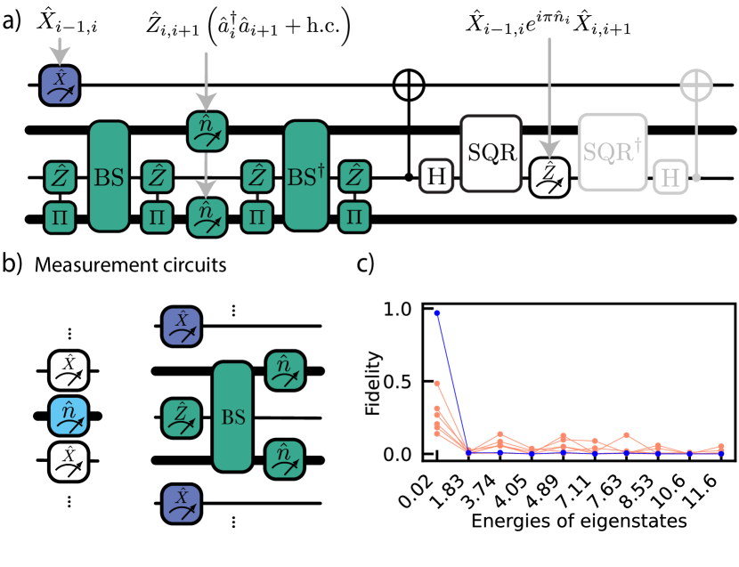
Figure 21: Ancilla-free post-selection methods based on Gauss’s law. a) Measurement circuit of the gauge-invariant hopping and electric field term (see Fig. 18c). It is adapted here in a way which enables a measurement of Gauss’s law at every site, black and white, in the same shot. The gates in gray are only required if more operations are to be carried out on the circuit. Because the measurement of Gauss’s law commutes with the one of the gauge-invariant hopping, they can be performed in either order. b) Measurement circuit of the density in light blue, required for calculating value of the onsite term. It commutes with $\hat{G}_{i}$, and we can therefore perform local checks of $\hat{G}_{i}$ using the measurement results, discarding shots that break Gauss’s law. The measurement of the gauge-invariant hopping (see Fig. 18c) does not commute with $\hat{G}_{i}$, and we therefore cannot conduct Gauss’s law checks for each site. However, the product $\hat{G}_{i}\hat{G}_{i+1}$ does commute with these circuits, allowing for post-selection upon Gauss’s law checks for pairs of sites. c) Fidelity $|\braket{\psi}{n}|^{2}$ of single quantum trajectories of the noisy simulation with the eigenstate $\ket{n}$ in our chosen Gauss’s law sector as a function of the eigenenergy. Trajectories that do not have overlap with states outside of the Gauss’s law sector are shown in blue, others are shown in red. Note that the shown fidelities of the states in red do not sum up to unity because we do not show the overlap with the states outside of our Gauss’s law sector. Energies are in units of $J$.

We simulate full Gauss’s law post-selection (the first scheme) and focus on its influence on the energy measurement. To do so, we take the final VQE parameters found in a noisy simulation (i.e. the final iteration of the black dots in Fig. 18) and run a simulation including hardware noise in the VQE circuit, but neglect noise in the measurement circuit. We then check whether an error happened in every quantum trajectory of the noisy simulation. The error-free trajectories exhibit high overlap $\approx 0.96\%$ with the ground state (c.f. blue line in Fig. 21c). For trajectories with an error, we project onto the correct Gauss’s law sector. The norm of the part of the wavefunction we project out gives us an estimate for the number of shots that would need to be discarded. We find that $13\%$ of shots need to be discarded. We show in red the overlap with the eigenstates in the correct Gauss’s law sector for some such states in Fig. 21c. Those states have still large overlap with the ground state, but also some overlap with excited states. To calculate the average post-selected energy, we renormalize the projected states and average over all trajectories. We find a post-selected energy of $0.36J$, compared to a result of $0.88J$ without post-selection and an exact ground-state energy of $E/J=0.02$. This corresponds to approx. $20\%$ of the difference between ground and first excited state energy.

In our simulations, we find that $84\%$ of quantum trajectories have no error. This is roughly in agreement with the dephasing survival probability of a single qubit, where $T_{2}=200\mu$s, only one of the qubits starts in $\ket{+}$, the other in $\ket{-}$, and the total circuit duration is $T=40\mu$s, which is $\exp(-T/T_{2})\approx 82\%$. These trajectories with no error have energy $0.16J$. The $1-84\%=16\%$ of trajectories in which an error happened therefore have average energy $4.66J$. Gauss-law post-selection reduces this average energy of the noisy trajectories to $1.41J$, where the remaining energy error results from noise processes within the same Gauss’s law sector. We therefore find that removing errors that bring us out of the correct Gauss’s law sector drastically reduces the energy error introduced by the noise.

More intricate mitigation methods can be engineered from this Gauss’s law check. For example, we note that one can cross-check $\hat{G}_{i}$ at different sites to not only detect that an error occured, but also resolve its position. This opens up the possibility to not only post-select on the case of no errors, but additional develop novel error-mitigation techniques where the error can be partially corrected. In addition, if the error is spatially disconnected in such a way that one can ascertain it did spread to a region of interest, then it may be desirable to retain this shot for the computation of observables local to this region. In addition to post-selection using gauge symmetries [183], VQE implementation for the $\mathbb{Z}_{2}$-Higgs model proposed here is amenable to other commonly used noise mitigation techniques such as zero-noise extrapolation [184, 185] and probabilistic error cancellation [184]. An alternative to post-selection is to introduce an additional term in the Hamiltonian which enforces the symmetry constraint by prethermalization [186], or pseudo-generators for gauge protection [187, 188].

VI.5 Measuring observables

Having characterised the hybrid oscillator-qubit VQE state preparation in terms of the energy error and overlap with the true ground state, we now show how to extract relevant observables in the proposed cQED architecture. While we benchmark the measurement of the observables for the ground state, the measurement schemes can in principle be applied to any state.

VI.5.1 Detecting phases of the $\mathbb{Z}_{2}$-Higgs model  in VQE-prepared ground states

In Fig. 22, we calculate different gauge-invariant observables in the $\mathbb{Z}_{2}$-Higgs model for varying onsite interaction, with respect to VQE ground states of a system with four bosonic sites and three gauge field sites found using noiseless simulations employing the SLSQP optimizer. We compare to exact diagonalisation results. We find that all VQE observables agree very well with the exact results, as expected from the low relative energy error found in Fig. 18 for this small system size.

Importantly, despite the small system size, we can see the hallmarks of three qualitatively different states as $U/J$ is scanned [137]. The three states are indicated by the blue (rightmost), red (middle) and yellow (leftmost) color of the lines, representing a Mott-insulating phase, pair superfluid phase and the “clump phase” – a phase in which the gauge field perturbatively generates a nearest-neighbour attraction between the bosons, leading to the bosons “clumping” together on the same site [137]. For four sites, we define the “clump order parameter” as the probability of all four bosons to occupy the same site (defined in caption of Fig. 22). This observable indeed becomes large for small $U/J$ [137]. A (Mott) insulating state is characterized by a lack of spreading of particles in the system. We observe signatures of this effect in the string order correlator and pair hopping, which are both small for large $U/J$. Moreover, on-site fluctuations are also small in the insulating state as expected. Finally, the parity tends towards $-1$, indicating that on average there is an odd occupation at each site. By contrast, in a superfluid phase, particles spread far. In the case of the $\mathbb{Z}_{2}$-Higgs model, single particles stay confined due to the presence of the gauge field while two particles can spread [137], which we observe in the large pair hopping and fluctuations. Moreover, contributions from states with a single boson are suppressed, which we see from the parity tending towards $+1$.

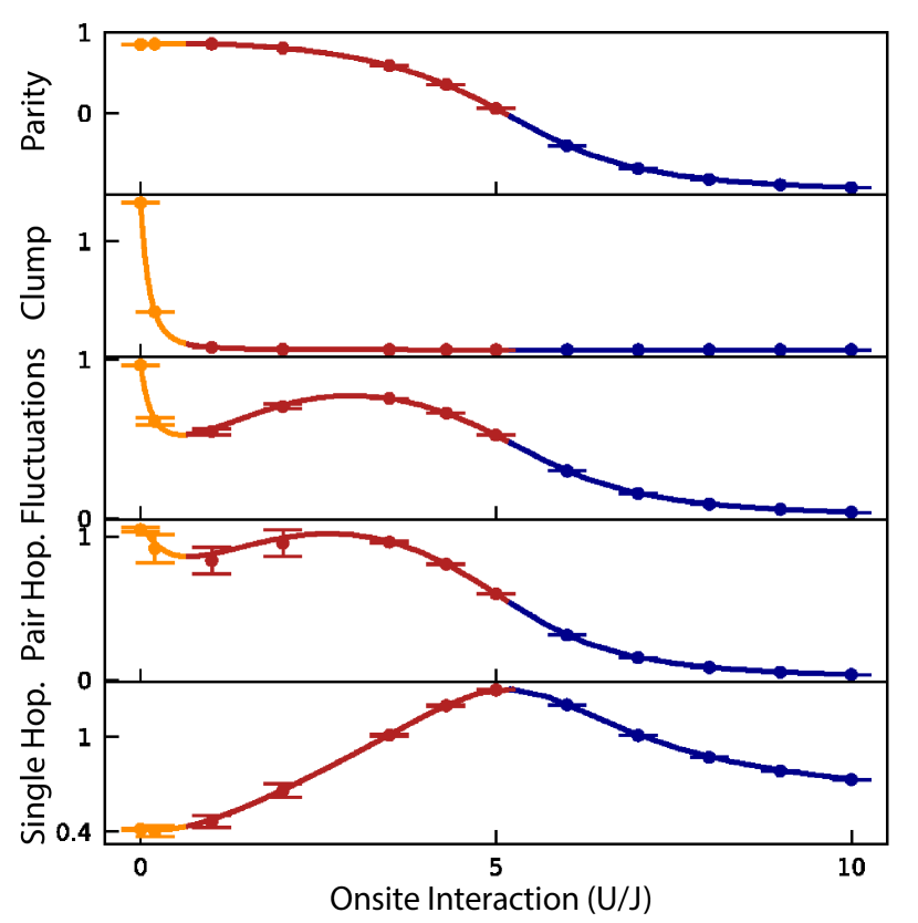
Figure 22: Correlation functions measured on the VQE ground state estimate. The observables are defined as follows. Parity: $\sum_{i}^{L}\langle e^{i\pi\hat{n}_{i}}\rangle/L$. Clump: $\sum_{i}^{L}\langle\hat{n}_{i}(\hat{n}_{i}-1)(\hat{n}_{i}-2)(\hat{n}_{i}-3)+\mathrm{h.c.}\rangle/L$. Fluctuations: $\sum_{i}^{L}(\langle\hat{n}_{i}\rangle^{2}-\langle\hat{n}_{i}^{2}\rangle)/L$. Pair hopping: $\sum_{i}^{L}\langle\hat{a}_{0}^{\dagger 2}\hat{a}_{i}^{2}+\mathrm{h.c.}\rangle/L$. string order correlator (also known as gauge-invariant string order correlator): $\sum_{i}^{L}\langle\hat{a}_{0}^{\dagger}\hat{Z}_{0}...\hat{Z}_{i}\hat{a}_{i}+\mathrm{h.c.}\rangle/L$. Four bosonic sites and three gauge field sites. Unit filling, i.e., four bosons are in the system. $g/J$=5. Error bars indicate standard deviation of five VQE simulations with four layers.

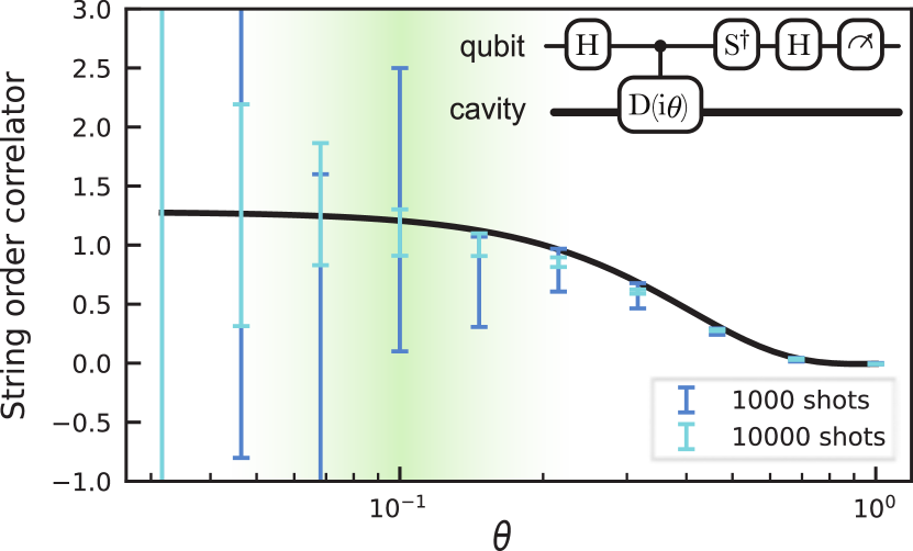
Figure 23: Measurement of the string order correlator as a function of the small angle $\theta$ chosen for the conditional displacement. (top right) Quantum circuit for measuring $\sin(k\hat{x})$ of an oscillator using the phase kickback of a conditional displacement [95]. (main plot) We run a full VQE simulation and measure the string order correlator using the scheme discussed in the main text, i.e., we measure the string order correlator approximated by the RHS of Eq. (177) by adding two ancilla qubits. The black line is obtained using exact SLSQP optimisation, the error bars are including shot noise, using SPSA optimisation. In both cases, we consider $3$ sites, $2$ gauge field links, $g/J=1$, $U/J=1$. The green highlight indicates the general region which optimizes for accuracy ($\theta$ small) and precision (the smaller $\theta$ is, the more shots are required to precisely measure the result).

Having shown that signatures of different phases can be found from VQE simulations, we now discuss how the different observables can be measured in our cQED architecture.

VI.5.2 Measuring the string order correlator

The gauge-invariant string order correlator is large in a deconfined phase and small in a confined phase. It is defined as $\braket{\hat{a}_{i}^{\dagger}\hat{Z}_{i,i+1}...\hat{Z}_{j-1,j}\hat{a}_{j}+\mathrm{h.c.}}$. To measure the value of this correlator on the ground states prepared via VQE, we need to correlate a measurement of the gauge field qubits with the measurement of the beamsplitter operator of two bosonic sites. We note that one possibility is to adapt the scheme used in Sec. VI.4.1 to measure a long-range hopping through the use of bosonic SWAPs. Ordinarily, such a measurement would require a time linear in the distance $|j-i|$. Alternatively, here we propose a separate strategy to measure this nonlocal observable using homodyne measurements: first, we expand $\hat{a}_{i}=(\hat{x}_{i}+i\hat{p}_{i})/2$, where $\hat{x}$ and $\hat{p}$ are the bosonic position and momentum operators respectively, such that

$$\braket{\hat{a}_{i}^{\dagger}\hat{Z}_{i,i+1}...\hat{Z}_{j-1,j}\hat{a}_{j}+\mathrm{h.c.}}$$

$$=\frac{1}{2}\left(\braket{\hat{x}_{i}\hat{Z}_{i,i+1}...\hat{Z}_{j-1,j}\hat{x}_{j}}+\braket{\hat{p}_{i}\hat{Z}_{i,i+1}...\hat{Z}_{j-1,j}\hat{p}_{j}}\right)$$ (173)

We must therefore perform correlated measurements of $\hat{x}_{i}$, $\hat{Z}_{i,i+1}$ and $\hat{x}_{j}$ (and, separately, $\hat{p}_{i}$, $\hat{Z}_{i,i+1}$ and $\hat{p}_{j}$). In order to measure $\hat{x}_{i}$, we use a Hadamard test implemented with a displacement conditioned on an ancilla, defined as $\mathrm{CD}(\alpha)=e^{\left(\alpha\hat{a}^{\dagger}-\alpha^{*}\hat{a}\right)\hat{Z}^{\mathrm{anc}}}$ (see Table 1). Choosing an arbitary real angle $\theta$ such that $\alpha=i\theta$, we get $\mathrm{CD}(i\theta)=e^{i\theta\hat{x}\hat{Z}^{\mathrm{anc}}}$. A measurement of the ancilla after applying the Hadamard test circuit with a small angle $\theta$, shown inside Fig. 23, then yields

$$\braket{\hat{Z}^{\mathrm{anc}}}_{\alpha=i\theta} =\braket{\left(\sin(2\theta\hat{x}\right)}$$ (174)

$$\approx 2\theta\braket{\hat{x}}+O(\theta^{3}).$$ (175)

To measure the first part of the string order correlator we perform two Hadamard tests simultaneously in order to correlate sites $i$ and $j$, i.e., after applying the Hadamard circuits on both sites $i$ and $j$ we measure

$$\braket{\hat{Z}^{\mathrm{anc}}_{i}\hat{Z}_{i,i+1}\dots\hat{Z}_{j-1,j}\hat{Z}^{\mathrm{anc}}_{j}}_{\alpha_{i}=\alpha_{j}=i\theta}$$

$$\approx 4\theta^{2}\braket{\hat{x}_{i}\hat{Z}_{i,i+1}\dots\hat{Z}_{j-1,j}\hat{x}_{j}}.$$ (176)

Similarly, we measure the second part of the string order correlator, i.e., those involving $\hat{p}$ correlations, by using conditional displacements with $\alpha=\theta$.

In summary, we get

$$\braket{\hat{a}_{i}^{\dagger}\hat{Z}_{i,i+1}...\hat{Z}_{j-1,j}\hat{a}_{j}+\mathrm{h.c.}}$$

$$\approx\frac{1}{8\theta^{2}}\big{(}\braket{\hat{Z}^{\mathrm{anc}}_{i}\hat{Z}_{i,i+1}\dots\hat{Z}_{j-1,j}\hat{Z}^{\mathrm{anc}}_{j}}_{\alpha_{i}=\alpha_{j}=i\theta}$$

$$\quad+\braket{\hat{Z}^{\mathrm{anc}}_{i}\hat{Z}_{i,i+1}\dots\hat{Z}_{j-1,j}\hat{Z}^{\mathrm{anc}}_{j}}_{\alpha_{i}=\alpha_{j}=\theta}\big{)}.$$ (177)

To test that we can be in the small $\theta$ regime while still being able to measure the string order correlator accurately with a reasonable number of shots, we simulate the measurement using Bosonic Qiskit, c.f. Fig. 23. We find that a choice of $\theta\approx 0.1$ suffices, requiring approximately $\frac{1}{\theta^{4}}=10^{4}$ shots, as expected from the statistical uncertainty of shot noise. Note that for this measurement, we do not need additional ancillae as one can recycle gauge link qubits that are not within the support of the string order correlator for this purpose. Lastly, we remark that one could alternatively use the method of quantum signal processing (see App. E) to extract $\langle\hat{x}\rangle$ similarly to Eq. (174), but with a larger value of $\theta$. This could be achieved by enacting a target function $\frac{2}{\pi}\arcsin(\cdot)$ on the signal $\sin(2\theta\hat{x})$; if $2\theta\hat{x}\leq 1/2$, this outputs $\frac{\theta}{\pi}\langle\hat{x}\rangle+O(\epsilon)$ while requiring $O(\log(1/\epsilon))$ queries to $\text{CD}(i\theta)$ [189].

VI.5.3 Measuring the superfluid density

The superfluid density $\rho_{s}$ in $1$D is given by [190, 191]

$$\rho_{s}=\frac{L}{J}\frac{\partial^{2}E_{\mathrm{TPB}}(\phi)}{\partial\phi^{2}},$$ (178)

where $E_{\mathrm{TPB}}(\phi)$ is the ground state energy in the presence of “twisted” periodic boundary conditions and $J$ is the hopping matrix element between neighbouring sites. The phase $\phi$ is given by the phase difference between two edges, for example for the $\mathbb{Z}_{2}$-Higgs model, we have

$$\hat{H}^{\textrm{TPB}}_{\mathbb{Z}(2)}(\phi)=\hat{H}_{\mathbb{Z}(2)}-J(e^{i\phi}\hat{a}_{L}^{\dagger}\hat{Z}_{n}\hat{a}_{1}+e^{-i\phi}\hat{a}_{L}\hat{Z}_{n}\hat{a}_{1}^{\dagger}),$$ (179)

where the entirety of the accumulated phase $\phi$ is incorporated by the hopping term between the two edge sites, where $\hat{H}_{\mathbb{Z}(2)}$ is defined in (151) and $L$ is number of sites. To measure $\braket{\hat{H}^{\textrm{TPB}}_{\mathbb{Z}(2)}}$, we can follow the general procedure outlined in section VI.4.1. The procedure to estimate the stiffness is as follows: we first prepare the ground state for a range of small values of $\phi$. We do so by extending the variational ansatz in Section VI.3.1 to incorporate edge-to-edge hopping. Once prepared, we estimate Eq. (178) via finite-difference methods or, alternatively, through more sophisticated, noise-resilient techniques such as parameter shift rules [192].

Experimentally, periodic boundary conditions are not required in the hardware to implement edge-to-edge hopping. It is sufficient to synthesize a conditional beamsplitter between the two end modes and leverage this for an edge-to-edge hopping term in the Hamiltonian. We can synthesize a beamsplitter between the edges of the chain using the bosonic $\operatorname{SWAP}$ gate defined in Tab. 2 to move the mode information from both edges of the chain to adjacent sites, carry out the required operation between the modes, and $\operatorname{SWAP}$ the information back.

VI.6 Qubit-boson ground state preparation with quantum signal processing

While above we employed the heuristic VQE approach to approximately prepare the ground state, new developments in an algorithm known as quantum signal processing (QSP) provide an alternative approach to ground state preparation with provable accuracy and guarantees. Here we provide a brief comparison of VQE and QSP for ground state preparation of the $\mathbb{Z}_{2}$-Higgs model.

Initially pioneered in Refs. [193, 194], QSP provides a systematic method to apply a nearly arbitrary polynomial transformation to a linear operator embedded in a unitary matrix [189], thus furnishing a unifying framework for quantum algorithms [57, 189]. In short, QSP works by interleaving the unitary matrix with a sequence of parameterizable SU(2) rotations; see Fig. 24 for an illustration. The output of this sequence is an embedding of a polynomial transformation of the initial linear operator, parameterized by the chosen SU(2) rotations. For a more detailed introduction to QSP, see App. E.

In App. F, we illustrate how QSP furnishes an algorithm for ground state preparation, as initially presented in Ref. [195] for implementation on early fault-tolerant quantum computers. In this scenario, one considers a Hamiltonian $H$ with spectral gap bounded below by $\Delta$, and seeks to prepare its ground state with fidelity $\geq 1-\epsilon$. As input to this algorithm, one assumes access to an easily preparable initial state that has overlap $\geq\gamma$ with the ground state. One also assumes access to the time evolution operators $e^{\pm iH}$, implemented for instance with Trotterization. To avoid alisiaing, it is taken that the eigenvalues of $H$ lie in the range $(0,\pi)$; othwerwise can implement a rescaled time evolution operator $e^{\pm i(H\Delta t+\phi)}$ to meet this constaraint.

With this setup, the algorithm uses QSP to approximate a projector onto the ground state, which is then applied to the initial state to project out its component parallel to the ground state. This algorithm ultimately requires a circuit depth $O\big{(}\frac{1}{\Delta}\log(1/\epsilon\gamma)\big{)}$, consisting of this many coherent queries to the controlled time evolution $e^{\pm iH}$. This circuit is repeated $O(\frac{1}{\gamma^{2}})$ times to prepare the ground state with high probability. The circuit of this algorithm is illustrated in Fig. 24.

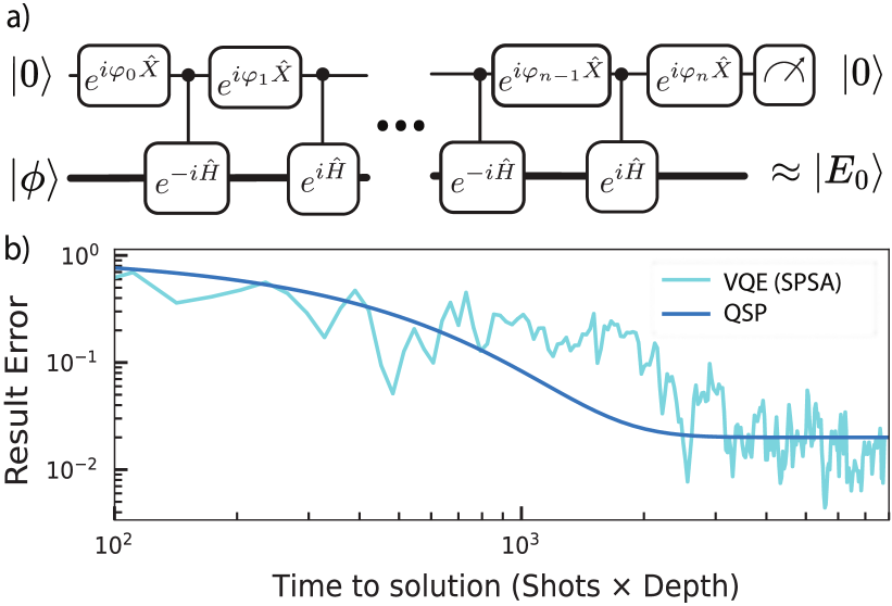
Figure 24: Considerations for ground state preparation using quantum signal processing. a) Circuit for ground state preparation with quantum signal processing, adapted from Ref. [195]. The parameters $\mathbf{\varphi}=(\varphi_{0},\varphi_{1},...,\varphi_{n})$ can be chosen such that upon post selecting on $|0\rangle$, the resulting state is a good approximation to the ground state $|E_{0}\rangle$. Note that this circuit interleaves $e^{\pm iH}$, distinct from the usual QSP construction; this modification is included to generate polynomial transformations in $\cos(H/2)$ (i.e., $P(\cos(H/2))$) and better approximate a projector onto the ground state subsapce. b) Fidelity with the exact ground state wavefunction vs. time to solution for VQE and QSP for the $\mathbb{Z}_{2}$-Higgs model for $U/J=1=g/J$, three bosonic sites, two gauge field sites. For VQE, the dominant error is the infidelity with the exact ground state; for QSP, the dominant error is the probability of failure. For details see App. F.

Recent work has shown that QSP is naturally implementable on hybrid CV-DV quantum procesors [45, 196], rendering it applicable to the LGT simulations studied here. To exemplify the requirements of ground state preparation with QSP, let us consider the $\mathbb{Z}_{2}$ model with $n=3$ sites and couplings $J=g=U=1$, as investigated in Sec. VI.4. Let us also use the same initial state as above, which numerically has overlap $\gamma\approx 0.36$ with the ground state. In this scenario, VQE produces the ground state with infidelity $\epsilon\approx 2\cdot 10^{-2}$ (see Fig. 20). Aiming to achieve a similar performance with QSP, our calculations in App. F indicate that the QSP approach requires $\sim 50$ queries to the controlled time evolution $e^{\pm iH}$. Using even a first order Trotterization as outlined in Sec. VI.2, a single such Trotter step would require $\sim 3$ controlled qubit-boson gates per site, for a rough total of $\gtrsim 10^{4}$ qubit-boson gates, which is prohibitively more expensive than VQE.

This prohibitive circuit depth suggests that QSP-based ground state preparation will only become practical and competitive with VQE once qubit-boson gate infidelities $\ll 10^{-4}$ can be achieved, in contrast to the current qubit-boson gate infidelities $\sim 10^{-3}$ [91, 197]. And moreover, even if such a gate fidelity can be achieved, the number of repetitions of the QSP circuit will generally scale exponentially in the system size without prior knowledge of the ground state (see App. F). However, this scaling is to be expected because generic ground state preparation is QMA-hard [198], and of course the VQE ground state preparation is also expected to require resources exponential in the system size, without further prior knowledge.

In Fig. 24, we compare the performance of VQE to QSP, as applied to the above scenario of the $\mathbb{Z}_{2}$ model. For both methods, we plot the dominant source of error vs. time to solution, assuming no gate errors in the underlying circuit. The dominant source of error for VQE is the infidelity with the ground state, and for QSP it is the probability of failure (see App. F for details); the time to solution is taken to be the circuit depth times the number of shots. For VQE, increasing the depth (i.e., number of layers) can increase the fidelity with the ground state, but also leads to a high dimensional optimisation problem that suffers from barren plateaus and requires a high shot count to facilitate optimisation [164]. On the other hand, QSP requires a relatively deeper circuit to estimate a projector onto the ground state, and a modest number of shots to successfully project out the ground state. Incidentally, the empirical results of Fig. 24 suggest that both dominant sources of error scale similarly as a function of the time to solution, implying that their total resource costs are comparable. This arises because our VQE circuit has a shallow depth yet requires many shots, whereas QSP has a deeper circuit yet requires fewer shots. We speculate that this seemingly universal behavior arises from the fact that the complexity of ground state preparation is fundamentally governed by the size of the spectral gap of the Hamiltonian, agnostic to the algorithm used to estimate the ground state. In any event, this analysis implies that VQE is better suited to settings with low gate fidelities and short coherence-times, whereas QSP is more favorable if gates are fast yet circuit repetitions are expensive.

VII Conclusions and outlook

To conclude, in this paper we have developed a resource-efficient framework for implementing fermion-boson quantum simulation of a wide variety of models including lattice gauge theories in $(1+1)$D and $(2+1)$D using oscillator-qubit quantum computation. To do so, we developed a range of compilation tools and subroutines to realize multi-body interaction terms using the natively available oscillator-qubit gate set in circuit QED hardware. In particular, we developed parity-controlled, and density-density bosonic gates and oscillator mediated multi-qubit gates as foundational subroutines, which are useful beyond our simulation motivation. In the context of LGTs, we showed how to implement gauge-invariant hopping terms for transmon and dual-rail qubit fermionic encodings. We also presented a method implementing the magnetic field term for $U(1)$ gauge fields.

By performing an end-to-end gate complexity analysis, including gate synthesis errors, we showed that our approach yields an asymptotic improvement from $\mathcal{O}(\log(S)^{2})$ to $\mathcal{O}(1)$ scaling in terms of the boson cutoff $S$ for the gauge-invariant hopping term and an $\mathcal{O}(\log(S))$ to $\mathcal{O}(1)$ improvement for the magnetic field term. Moreover, in order to also compare the prefactors of the compilation, we developed an efficient all-qubit algorithm in the Fock-binary encoding for simulating bosonic hopping terms. We show that even this efficient approach yields gate counts that are $10^{4}$ times higher than our oscillator-qubit approach.

We then applied our compilation strategies to some of the most pertinent quantum simulation tasks – ground state preparation and time evolution, for which we developed a oscillator-qubit variational quantum eigensolver method. We benchmarked our hybrid oscillator-qubit approach through numerical simulations of a $\mathbb{Z}_{2}$-Higgs model and $U(1)$ quantum link model in $(1+1)$D in Bosonic Qiskit, and demonstrated that low-depth oscillator-qubit circuits can prepare states with a high overlap with the ground state for small systems. In particular, in the $U(1)$ quantum link model we found relative energy errors of $<10^{-3}$ for just a two-layer ansatz for three matter sites. Separately, we simulated both the time dynamics and VQE for the $\mathbb{Z}_{2}$-Higgs model in the presence of the leading source of noise in circuit QED architectures – transmon decay and dephasing. We then developed an approach for post-selecting on Gauss’s law in VQE circuits, using the fact that each term in the Hamiltonian individually conserves Gauss’s law, and showed that energy errors of $20\%$ of the difference between ground and first excited state can be reached with this method. We also showed how non-trivial observables can be measured within our approach, including the superfluid stiffness and string order correlators. Finally, we discussed how quantum signal processing – an alternative approach to eigenstate preparation with performance guarantees – can be implemented in oscillator-qubit systems, showing that its time to solution for a fixed error is comparable to VQE.

Prospect for quantum advantage

For simulations in the NISQ-era, it is important that errors do not completely destroy the signal to be observed. In cavities, the probability of a Fock state $\ket{N}$ to decay to $\ket{N-1}$ scales linearly with $N$, therefore posing a challenge to the achievable fidelity for large $N$, in particular in the context of quantum computation (see e.g. section IIE2 in Ref. [45]). By contrast, when mapping bosons to qubits using the Fock-binary encoding, the probability to be in an encoded Fock state $\ket{N}$ has a decay-rate which scales as $\Omega(1)$ and $\mathcal{O}(\log_{2}(N))$. However, this apparent advantage of the Fock-binary encoding does not directly materialize when considering observables. As we discuss in App. G, for both cavities and qubits, even non-linear observables such as $\braket{\hat{n}^{2}}$ have a decay rate which is $\mathcal{O}(1)$ in $N$. This is in analogy to the fact that for many-qubit systems, local observables can have low error even when the global fidelity of the state is essentially zero [199, 200]. Therefore, the linearly growing decay rate of number states in cavities need not lead to particular difficulties for quantum simulation when considering such local observables. Moreover, the effective errors induced by qubit decay in the Fock-binary encoding are highly non-linear in $N$ and also lead to large jumps in occupations. For example, Fock states with $N=2^{n}$, $n\in\mathbb{N}$, decay immediately to $N=0$, leading to an effective loss of $2^{n}$ bosons at once. Hamiltonian evolution with non-linear terms such as an on-site interaction in the presence of Fock-state-dependent loss can lead to highly correlated errors. This is not the case for bosonic hardware, where the decay rate of $\braket{\hat{n}^{2}}$ for an initial Fock state is a smooth function of the Fock state number and in a single decay event, only a single boson is lost. Finally, in cavity QED, boson loss is far slower (decay rate $\kappa\approx 1$ kHz, with some cavities shown to exhibit $\kappa<1$ Hz) than qubit decay (decay rate $\gamma\approx 5-10$ kHz). The excellent coherence of cavities is illustrated by the recent experimental preparation of coherent (i.e., definite parity) photon cat states with as many as $1000$ photons [77]. Therefore, the differing nature of errors in oscillators, which is closer to physical errors appearing in bosonic systems, can pose advantages for qubit-boson hardware compared to all-qubit simuluations of bosonic systems.

As to the prospect of quantum advantage, we believe that non-equilibrium dynamics in regimes with large boson number fluctuations, starting in Fock states, will be challenging to simulate classically: the widely-used time-evolving-block-decimation algorithm for tensor networks scales cubically with the boson number cutoff [201]. Monte-Carlo methods struggle with non-equilibrium and real-time dynamics, while semi-classical methods such as the truncated Wigner approximation [202] with initial states that are non-Gaussian. Finally, brute-force sparse diagonalization methods struggles with large systems – we expect dynamics of system sizes of $L>20$ bosonic sites with an average of two bosons per site to be challenging to simulate when considering initial states leading to large boson fluctuations such as $\ket{0\cdots 0LL0\cdots 0}$, in which case the cutoff needs to be chosen to be essentially given by the number of bosons in the system, $2L$, leading to a Hilbert space size of $\binom{3L-1}{2L}$. The largest simulations to date have reached Hilbert space sizes of $<2^{40}$ [203]. Hence, we expect to surpass classical simulability using sparse matrix methods for $L\approx 16$. This is in contrast to qubit-only simulations, where systems of $L\gtrsim 50$ are needed to reach beyond-classical regimes [204].

Future directions

Our study opens a promising pathway towards using native oscillator-qubit hardware to simulate boson-fermion-gauge field systems. Compared to qubit-based hardware, this approach will be most advantageous when simulating systems with strong boson number fluctuations, for example in chaotic field theory evolution [205], as such a case requires large cutoffs and, consequently, the synthesis of square-root factors (when acting with creation and annihilation operators) that are expensive to synthesize in all-qubit hardware. A key advantage of our digital approach compared to classical or analog methods is its versatility – our approach can simulate topologies that do not match the hardware topology. For example, a $3$D model can in principle be mapped to the $2$D array at the expense of needing to implement long-range entangling gates with SWAPs.

Extending our approach to non-Abelian Gauge theories, most importantly $SU(N)$ to simulate the weak and strong forces, are most pertinent. To this end, our Schwinger-Boson approach can be relatively straightforwardly generalized [65, 206] and we expect similar scaling advantages to materialize as we found for $U(1)$ fields.

Many applications of qubit-oscillator quantum simulation such as vibronic excitations of molecules or phonon-electron interactions in condensed-matter physics show similar decoherence processes to the one present in qubit-oscillator hardware. This opens up the direction of hybrid qubit-oscillator digital simulation of open-system dynamics, which would be an interesting topic to explore next. In noisy qubit hardware, this would not be immediately possible as the physical loss processes do not resemble boson loss in Fock-binary encodings as discussed above.

Looking into the future beyond noisy simulations, our work motivates the study of bosonic error-correcting codes, i.e., codes that directly encode a bosonic logical operator. Furthermore, it would be interesting to explore, whether our proposed hybrid oscillator-qubit approach also yields advantages for equilibrium state preparation away from the ground state. To that end, quantum signal processing [57], methods based on filtering [207, 208, 209, 210], or thermalization [211, 212] could be employed. Another interesting direction is to develop explicit benchmarks of dynamical quantum simulations of, e.g., string breaking and particle scattering problems [40, 213] to better compare hybrid oscillator-qubit and qubit-based approaches.

While challenging in cavity QED hardware, a purely native approach for fermion-boson problems could be explored by combining our approach with digital fermionic quantum processing in neutral atom arrays [214, 42], where bosons can be encoded in (the mechanical) harmonic oscillator degrees of atoms in tweezers [56, 45].

VIII Acknowledgments

This research was funded by the U.S. Department of Energy, Office of Science, National Quantum Information Science Research Centers, Co-design Center for Quantum Advantage (C2QA) under contract number DE-SC0012704. C2QA led this research. Support is also acknowledged from the U.S. Department of Energy, Office of Science, National Quantum Information Science Research Centers, Quantum Systems Accelerator. S.K. is supported with funds from the Ministry of Science, Research and Culture of the State of Brandenburg within the Centre for Quantum Technologies and Applications (CQTA). J.M.M. acknowledges support from the National Science Foundation Graduate Research Fellowship under Grant No. 2141064. L.F. is supported by the Deutsche Forschungsgemeinschaft (DFG, German Research Foundation) as part of the CRC 1639 NuMeriQS – project no. 511713970.

We acknowledge helpful discussions with Marko Cetina, Zohreh Davoudi, Alexey Gorshkov, Fabian Grusdt, Mohammad Hafezi, Or Katz, and Torsten Zache.

External interest disclosure: SMG is a consultant for, and equity holder in, Quantum Circuits, Inc.

Appendix A Implementing fermionic Hamiltonian terms

A.1 Hopping

In this appendix we remind the reader of an existing approach for digitally simulating fermionic Hamiltonian terms which we show is feasible in hybrid qubit-oscillator hardware and simulation.

To take into account the negative sign in the many-body wavefunction appearing when two fermions exchange position, we employ the Jordan-Wigner [215] (JW) mapping (although many mappings would be possible, such as Bravyi-Kitaev [216], parity basis [217], etc.) The JW mapping fixes a reference site, defining a one-dimensional chain embedded in a $D$-dimensional volume and trailing a set of $\hat{Z}$ operators with each application of a fermionic creation or destruction operator along the chain:

$$\hat{c}_{i}^{\dagger}=\left(\bigotimes_{k=1}^{i-1}\hat{Z}_{k}\right)\otimes\hat{\sigma}_{i}^{+},\quad\hat{c}_{i}=\left(\bigotimes_{k=1}^{i-1}\hat{Z}_{k}\right)\otimes\hat{\sigma}_{i}^{-},$$ (180)

where $\hat{\sigma}^{-}=\frac{\hat{X}+i\hat{Y}}{2},\hat{\sigma}^{+}=\frac{\hat{X}-i\hat{Y}}{2}$.

For a one-dimensional system and only nearest-neighbour hopping, the strings of $\hat{Z}$ operations cancel out and $\hat{c}_{i}^{\dagger}\hat{c}_{i+1}+\mathrm{h.c.}$ reduces to $\hat{\sigma}_{i}^{+}\hat{\sigma}_{i+1}^{-}+\mathrm{h.c.}$. However, for $D>1$, the strings of $\hat{Z}$ only cancel if the hopping is between neighboring sites along the JW chain, but do not cancel if the two sites are not nearest neighbors along the JW chain.

A highly parallelized way of implementing hopping terms $e^{i2\theta\left(\hat{c}_{i}^{\dagger}\hat{c}_{j}+\mathrm{h.c.}\right)}$ between sites $i$ and $j$ that are not adjacent along the JW chain is a fermionic SWAP (FSWAP) network [113] (see e.g., Ref. [116] for a large-scale implementation). This idea uses FSWAP gates

$$\mathrm{FSWAP}_{i,j}=\mathrm{SWAP}_{i,j}\cdot\mathrm{CZ}_{i,j},$$ (181)

to bring every pair of fermions to Jordan-Wigner adjacent sites in exactly depth $N$, where $N$ is the number of fermions. When fermions are on adjacent sites, hopping is implemented using $\operatorname{iSWAP}(\theta)$ gates. This way, all hopping gates can be implemented in depth $N$, using $\mathcal{O}(N^{2})$ FSWAP gates and $N$ $\operatorname{iSWAP}(\theta)$ gates. This can be reduced to depth $\sqrt{N}$ for nearest-neighbour hopping on the 2D lattice.

We now comment on the transpilation of the required gates in terms of $ZZ(\theta)$ and single-qubit gates.

SWAP_i,j fully exchanges the contents of the sites $i$ and $j$ on which it is applied, and CZ is the conditional-Z gate. CZ applies $\hat{Z}$ on the second qubit only if the first is in $\ket{1}$ (which happens to be symmetric). This corresponds to the unitary $\operatorname{CZ}_{1,2}=\frac{1}{2}\left((\mathds{1}_{1}+\hat{Z}_{1})\mathds{1}_{2}+(\mathds{1}_{1}-\hat{Z}_{1})\hat{Z}_{2}\right)$. We have that $\operatorname{CZ}_{1,2}=e^{i\frac{\pi}{4}}e^{-i\frac{\pi}{4}\hat{Z}_{1}}e^{-i\frac{\pi}{4}\hat{Z}_{2}}e^{i\frac{\pi}{4}\hat{Z}_{1}\hat{Z}_{2}}$.

The Jordan-Wigner-adjacent hopping must be implemented, which is given by

$$\operatorname{iSWAP}_{i,j}(\theta) =e^{i\theta(\hat{\sigma}_{i}^{+}\hat{\sigma}_{i+1}^{-}+h.c)}$$

$$=e^{\-i\theta\left(\hat{X}_{i}\hat{X}_{i+1}\right)}e^{\-i\theta\left(\hat{Y}_{i}\hat{Y}_{i+1}\right)}.$$ (182)

Both $e^{\-i\theta\left(\hat{X}_{i}\hat{X}_{i+1}\right)}$ and $e^{\-i\theta\left(\hat{Y}_{i}\hat{Y}_{i+1}\right)}$ can be implemented by combining the $\operatorname{ZZ}_{i,j}(\theta)$ with single-qubit rotations using that $\hat{X}=\hat{H}\hat{Z}\hat{H}$ and $\hat{Y}=\hat{S}\hat{H}\hat{Z}\hat{H}\hat{S}^{\dagger}$, where $S=e^{i\pi/4}R^{Z}(\frac{\pi}{2})$. Furthermore, we note that when following $e^{\-i\theta\left(\hat{X}_{i}\hat{X}_{i+1}\right)}$ directly with $e^{\-i\theta\left(\hat{Y}_{i}\hat{Y}_{i+1}\right)}$, both dual-rail qubits have $\hat{H}\hat{S}\hat{H}$ applied to them, which reduces to $\frac{1}{2}[(1+i)\mathds{1}+(1-i)\hat{X}]=\operatorname{R}^{0}(\pi)$, a rotation around the $\hat{X}$ axis. Therefore, the iSWAP operation will require single qubit rotations and ZZ$(\theta)$ gates. These are the only two operations required to implement fermionic hopping using fermionic SWAP networks.

A.2 Onsite potential

On-site potential terms for fermions take the form $\sum_{i}\mu_{i}\hat{n}_{i}$ where $\hat{n}_{i}=\hat{c}^{\dagger}_{i}\hat{c}_{i}$. The time evolution of this term $e^{-i\mu_{i}t\hat{n}_{i}}$ can be mapped to single-qubit phase gates acting on each site individually, because $\hat{n}=(\mathds{1}-\hat{Z})/2$. These terms are not affected by the Jordan-Wigner mapping.

A.3 Onsite and intersite interactions

Intersite interactions take the form $\hat{H}=\sum_{\braket{i,j}}V_{i,j}\hat{n}_{i}\hat{n}_{j}$. The time evolution under this Hamiltonian $e^{iJt\sum_{\braket{i,j}}\hat{n}_{i}\hat{n}_{j}}$ can be mapped to $\operatorname{ZZ}_{i,j}(V_{i,j}t/2)$ gates combined with single-qubit phase gates in the JW mapping using $\hat{n}_{\mathrm{qubit}}=(\mathds{1}-\hat{Z})/2$. For multi-component models such as the Fermi-Hubbard model in which each site can for example have a spin-up fermion and/or a spin down fermion, the different components are mapped onto different qubit sites. Therefore, also on-site interactions $\hat{H}=U\sum_{\braket{i}}\hat{n}_{i,\alpha}\hat{n}_{i,\beta}$ between different components $\alpha$ and $\beta$ can be implemented using the $\operatorname{ZZ}_{i,j}(Ut/2)$ gate.

Appendix B Ancilla-free implementation of bosonic on-site interactions in the $(1+1)$D $\mathbb{Z}_{2}$-Higgs model 

In this section, we discuss the ancilla-free implementation of time-evolution for the bosonic on-site interaction term in the $\mathbb{Z}_{2}$-Higgs model. Our motivation for developing this scheme is that in the $(1+1)$D case in Section VI, each transmon dispersively coupled to a cavity encodes a matter degree of freedom, and is therefore not “available” as an ancilla for the realization of on-site interactions using the method of Section III.1.3. While experiments have successfully incorporated multiple transmons per cavity [218], such a strategy is challenging and outside of the proposed architecture in Fig. 2.

In this section, we discuss a workaround for realizing this term that relies on Gauss’s law. For simplicity, we describe this strategy in the context of the $(1+1)$D $\mathbb{Z}_{2}$-Higgs model, but note that an extension to $(2+1)$D is possible. In particular, we develop an exact, ancilla-free implementation of arbitrary onsite interactions using one qubit per cavity while also preserving the quantum information in each qubit.

This approach leverages a combination of SNAP gates, Mølmer-Sørensen-like multi-qubit gates discussed in Section II.6, and Gauss’s law constraints. The key idea is to introduce an identity in the form of Gauss’s law, for which we use the convention,

$$\hat{G}_{i}=\hat{X}_{i-1,i}\>e^{i\pi\hat{n}_{i}}\>\hat{X}_{i,i+1}=+\mathds{1},$$ (183)

to rewrite

$$e^{-iU\hat{n}_{i}^{2}t}=e^{-i\left(\hat{X}_{i-1,i}e^{i\pi\hat{n}_{i}}\hat{X}_{i,i+1}\right)U\hat{n}_{i}^{2}t},$$ (184)

where symbols are as defined in Sec. III.1.3.

To synthesize the right-hand side using native gates, we recast it as

$$e^{-i\hat{X}_{i-1,i}\hat{X}_{i,i+1}\sum_{n}\theta_{n}\ket{n}\bra{n}_{i}}=\hat{V}^{\dagger}e^{-i\hat{Z}_{i,i+1}\sum_{n}\theta_{n}\ket{n}\bra{n}_{i}}\hat{V}$$ (185)

in terms of the Fock states $\ket{n}$ with number eigenvalue $n$ and the angles are defined as $\theta_{n}=e^{i\pi n}Un^{2}t$. The right hand side of the equality in (185) corresponds to a $\operatorname{SNAP}$ gate defined in Tab. 1, conjugated by the two-qubit unitary

$$\hat{V}=\hat{H}_{i,i+1}e^{i\frac{\pi}{4}\left(\mathds{1}_{i-1,i}-\hat{X}_{i-1,i}\right)\hat{Z}_{i,i+1}},$$ (186)

where $\hat{H}_{i,i+1}$ is a Hadamard gate on the qubit linking sites $i$ and $i+1$, and $\mathds{1}_{i,i+1}$ the identity. Therefore, synthesis of this term reduces to the task of implementing of $\hat{V}$, which is possible in the proposed architecture through use of the Mølmer-Sørensen-like scheme introduced in Ref. [45]. The exact circuit that realizes $\hat{V}$ is shown in Fig. 25.

While this approach enables us to implement arbitrary on-site interactions without additional ancillas, it is important to note that its reliance on Gauss’s law can result in the propagation of photon-loss and qubit dephasing errors as effective gate errors. However, such effects can be at least partially mitigated by post-selecting results on states which satisfy or partially satisfy Gauss’s law (which we discuss in Sec. VI.4.5). Note that this will however come at the cost of an increased number of shots that scales exponentially with system size.

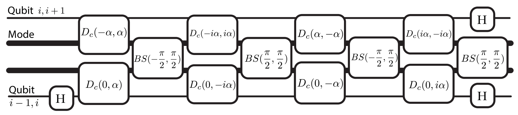
Figure 25: Circuit for implementing the unitary $V$ defined in Eq. 186. This enables an ancilla-free implementation of on-site interactions in the $(1+1)$D $\mathbb{Z}_{2}$-Higgs model for the choice $\alpha=\frac{1}{2}\sqrt{\frac{\pi}{2}}$. In the above, $\operatorname{D_{c}}(\beta,\gamma)=\ket{0}\bra{0}\otimes\operatorname{D}(\beta)+\ket{1}\bra{1}\otimes\operatorname{D}(\gamma)$ is an asymmetric conditional displacement (see Ref. [45] for details), where $\operatorname{D}(\cdot)$ is an unconditional displacement as defined in Table 1.

Appendix C Realizing three-wave mixing Hamiltonians with driven sideband transitions

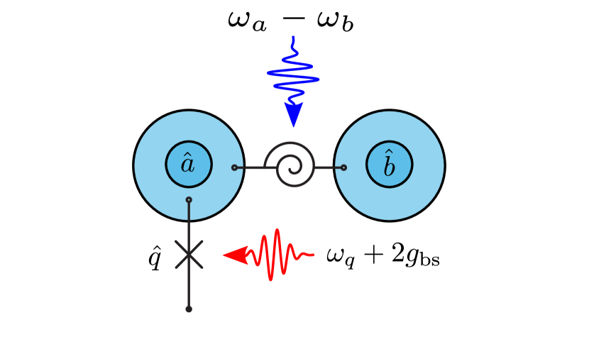
Figure 26: Realization of an effective three-wave mixing term. Two nodes of the proposed superconducting architecture consisting of a transmon, two cavities, and a tunable beamsplitter interaction. The second transmon coupled to cavity $b$ is not shown. The SNAIL mixing element is driven at $\omega_{a}-\omega_{b}$ to hybridize modes $a$ and $b$. In addition, a sideband drive at frequency $\omega_{q}+2g_{\text{bs}}$ is applied to the transmon, activating the desired three-wave mixing interaction.

In this section, we outline one possible method for realizing the three-wave mixing terms needed for gauge-invariant fermonic hopping as described in IV.5.2. The goal here is to realize the two Hamiltonians

$$E=\left(ab^{\dagger}\sigma_{b}^{+}+a^{\dagger}b\sigma_{b}^{-}\right)/2$$ (187)

$$F=i\left(ab^{\dagger}\sigma_{b}^{+}-a^{\dagger}b\sigma_{b}^{-}\right)/2.$$ (188)

We focus on two nodes of the proposed experimental architecture as shown in Fig. 26. Here, an ancilla qubit $q$ (transmon) at frequency $\omega_{q}$ is coupled to an oscillator $a$ with vacuum Rabi rate $2g_{qa}$. Oscillator $a$ is coupled to oscillator $b$ with a tuneable beamsplitter interaction $g_{\text{bs}}(t)$ activated by a pumped three-wave mixing element with pump frequency $\omega_{p}$. The second transmon, coupled to cavity $b$, can be dynamical decoupled during the interaction.

By activating the beamsplitter between modes $a$ and $b$ while simultaneously driving a sideband on qubit $q$, we can achieve the desired three-wave coupling. Here, the sideband frequency should be $\omega_{q}+2g$, blue-detuned by the mode splitting between $a$ and $b$ when the beamsplitter is activated.

In the lab frame, expanding the junction’s cosine potential to fourth order, the relevant effective Hamiltonian for the three modes can be approximated as

$$H_{0}/\hbar =\omega_{a}a^{\dagger}a+\omega_{b}b^{\dagger}b+\omega_{q}q^{\dagger}q$$ (189)

$$\quad+g_{\text{bs}}\left(a^{\dagger}be^{-i\omega_{p}t}+ab^{\dagger}e^{i\omega_{p}t}\right)$$

$$\quad+g_{qa}\left(a^{\dagger}q+aq^{\dagger}\right)-\frac{E_{J}}{4!}\left(\varphi_{q}\left(q+q^{\dagger}\right)\right)^{4}$$

where $\varphi_{q}=\left(\frac{2E_{C}}{E_{J}}\right)^{\frac{1}{4}}$ and $\omega_{p}$ is the beamsplitter pump frequency.

To analyze this Hamiltonian, we first apply a dispersive transformation on modes $q$ and $a$. Assuming $g\ll\Delta_{qa}$, we expand to first order in $\frac{g_{qa}}{\Delta}$ to find

$$H_{1}/\hbar =\omega_{a}a^{\dagger}a+\omega_{b}b^{\dagger}b+\omega_{q}q^{\dagger}q$$ (190)

$$\quad+g_{\text{bs}}\left(a^{\dagger}be^{-i\omega_{p}t}+ab^{\dagger}e^{i\omega_{p}t}\right)$$

$$\quad-\frac{E_{J}}{4!}\left(\varphi_{q}\left(q+q^{\dagger}\right)+\varphi_{q}\frac{g_{qa}}{\Delta_{qa}}\left(a+a^{\dagger}\right)\right)^{4}$$

where we have redefined $\omega_{a}$, $\omega_{b}$, and $\omega_{q}$ to be the normalized mode frequencies.

Driving the beamsplitter on resonance corresponds to a SNAIL pump frequency of $\omega_{p}=\omega_{b}-\omega_{a}$. Moving into the rotating frame of modes $a$, $b$, and $q$, we find

$$\tilde{H_{1}}/\hbar =g_{\text{bs}}\left(a^{\dagger}b+ab^{\dagger}\right)$$ (191)

$$\quad-\frac{E_{J}}{4!}\left(\varphi_{q}\left(qe^{-i\omega_{q}t}+q^{\dagger}e^{i\omega_{q}t}\right)\right.$$

$$\quad\left.+\varphi_{q}\frac{g_{qa}}{\Delta_{qa}}\left(ae^{-i\omega_{a}t}+a^{\dagger}e^{i\omega_{a}t}\right)\right)^{4}$$

From here, we make a Bogoliubov transformation $\tilde{H}_{2}=U^{\dagger}\tilde{H}_{1}U$ where $U=\exp\left(\frac{\pi}{4}(a^{\dagger}b-ab^{\dagger})\right)$, leading to

$$\tilde{H}_{2} =g_{\text{bs}}\left(b^{\dagger}b-a^{\dagger}a\right)$$ (192)

$$\quad-\frac{E_{J}}{4!}\left(\varphi_{q}\left(qe^{-i\omega_{q}t}+q^{\dagger}e^{i\omega_{q}t}\right)\right.$$

$$\quad\left.+\varphi_{q}\frac{g_{qa}}{2\Delta_{qa}}\left(\left(a+b\right)e^{-i\omega_{a}t}+\left(a^{\dagger}+b^{\dagger}\right)e^{i\omega_{a}t}\right)\right)^{4}.$$

Finally, we can account for the mode splitting of $2g_{bs}$ by moving into the rotating frame of $a$ and $b$ at frequencies $\mp g$ to find

$$\tilde{H}_{3} =-\frac{E_{J}}{4!}\bigg{[}\varphi_{q}\left(qe^{-i\omega_{q}t}+q^{\dagger}e^{i\omega_{q}t}\right)$$ (193)

$$\quad+\varphi_{q}\frac{g_{qa}}{2\Delta_{qa}}\bigg{(}ae^{-i\left(\omega_{a}-g\right)t}+be^{-i\left(\omega_{a}+g\right)t}$$

$$\quad+a^{\dagger}e^{i\left(\omega_{a}-g\right)t}+b^{\dagger}e^{i\left(\omega_{a}+g\right)t}\bigg{)}\bigg{]}^{4}$$

Here, we see that by activating a resonant beamsplitter between mode $a$ and $b$, the transmon mode $q$ has an effective four-wave coupling to both mode $a$ and $b$, seen by the qubit at effective frequencies $\omega_{a}\pm g$. Given this, we can drive the qubit with a sideband drive at frequency $\omega_{d}=\omega_{q}+2g$ to activate the desired three-wave mixing term. To see this, we add a drive term with strength $\xi$,

$$\tilde{H}_{3} =-\frac{E_{J}}{4!}\bigg{[}\varphi_{q}\left(qe^{-i\omega_{q}t}+q^{\dagger}e^{i\omega_{q}t}\right)$$ (194)

$$\quad+\varphi_{q}\frac{g_{qa}}{2\Delta_{qa}}\bigg{(}ae^{-i\left(\omega_{a}-g\right)t}+be^{-i\left(\omega_{a}+g\right)t}$$

$$\quad+a^{\dagger}e^{i\left(\omega_{a}-g\right)t}+b^{\dagger}e^{i\left(\omega_{a}+g\right)t}$$

$$\quad+\xi e^{-i\omega_{d}t}+\xi^{*}e^{i\omega_{d}t}\bigg{)}\bigg{]}^{4}$$

and expand the four-wave mixing term. We find the desired resonant process

$$\tilde{H}_{\text{sideband}}/\hbar=-E_{J}\varphi_{q}^{3}\left(\frac{g_{qa}}{2\Delta_{qa}}\right)^{2}\left(\xi ab^{\dagger}q^{\dagger}+\xi^{*}a^{\dagger}bq\right).$$ (195)

To avoid driving other undesired terms, the strength of the process must be small with respect to the mode splitting, $2g_{\text{bs}}$. Further analysis of this process in an experimental setting will be needed to solidify its use as a viable path to realizing effective three-wave mixing. Other methods could be also be used, such as a dedicated four-wave mixing element coupling modes $q$, $b$, and $a$.

Appendix D Qubit gate counts for simulating a beamsplitter Hamiltonian

In this appendix, we explain how to obtain the number of two-qubit gates necessary for compiling a beamsplitter between two modes $e^{-i\theta\hat{H}}$ with

$$\hat{H}=\hat{a}^{\dagger}b+\hat{a}\hat{b}^{\dagger}$$ (196)

onto a qubit-only quantum computer within the Fock-binary encoding. We do this by generalising the calculation presented in Appendix F of Ref. [45] which presents the compilation of a displacement on a single mode $e^{-i(\alpha\hat{a}^{\dagger}-\alpha^{*}\hat{a})}$, where $\alpha$ is a complex number.

The beamsplitter can be divided into four parts according to $H=(H_{\mathrm{even},\mathrm{even}}+H_{\mathrm{even},\mathrm{odd}}+H_{\mathrm{odd},\mathrm{even}}+H_{\mathrm{odd},\mathrm{odd}})$. The four parts contain matrix elements which are square roots of products of even/odd numbers. For example, $H_{\mathrm{even},\mathrm{odd}}$ only contains matrix elements with value $\sqrt{x\times y}$, where $x$ is even and $y$ is odd. This corresponds to those parts of the Hamiltonian where $\hat{a}^{\dagger}\hat{b}$ acts on Fock states $\ket{\mathrm{odd}}\ket{\mathrm{odd}}$ transforming them to $\sqrt{\mathrm{even}\times\mathrm{odd}}\ket{\mathrm{even}}\ket{\mathrm{even}}$, and $\hat{a}\hat{b}^{\dagger}$ acts on Fock states $\ket{\mathrm{even}}\ket{\mathrm{even}}$ transforming them to $\sqrt{\mathrm{even}\times\mathrm{odd}}\ket{\mathrm{odd}}\ket{\mathrm{odd}}$:

$$\hat{a}^{\dagger}\hat{b}\ket{2j+1}\ket{2l+1}= \sqrt{2(j+1)\times 2l+1}\ket{2(j+1)}\ket{2l}$$ (197)

$$\hat{a}\hat{b}^{\dagger}\ket{2(j+1)}\ket{2l}= \sqrt{2(j+1)\times 2l+1}\ket{2j+1}\ket{2l+1}.$$ (198)

The action of $H_{\mathrm{even},\mathrm{odd}}$ rotates between the states: $\ket{2j+1}\ket{2l+1}$ and $\ket{2(j+1)}\ket{2l}$.

We can therefore decompose, using a first-order Trotter formula, the time evolution under a beamsplitter into four parts:

$$e^{-i\theta\hat{H}} =e^{-i\theta\hat{H}_{\mathrm{even},\mathrm{even}}}e^{-i\theta\hat{H}_{\mathrm{even},\mathrm{odd}}}e^{-i\theta\hat{H}_{\mathrm{odd},\mathrm{even}}}e^{-i\theta\hat{H}_{\mathrm{odd},\mathrm{odd}}}$$

$$+\mathcal{O}(\theta^{2}).$$ (199)

This reduces the problem to compiling time evolution under the four parts individually.

Crucially, these four parts are one-sparse matrices within the Fock-binary encoding and can be decomposed into direct sums of terms which are a constant times a $\hat{\sigma}^{x}$ Pauli matrix. This will enable us in the following to map the evolution under this Hamiltonian to a rotation on a single ancilla qubit. For example, in the case of $H_{\mathrm{even},\mathrm{odd}}$, the amplitudes of $\ket{2j+1}\ket{2l+1}$ and $\ket{2(j+1)}\ket{2l}$ will be mapped to the amplitudes of $\ket{0}$ and $\ket{1}$ of an ancilla qubit, and a single qubit rotation will effectively carry out the action of $H_{\mathrm{even},\mathrm{odd}}$. We explain this in more detail in the following.

We divide the state of the two modes into even and odd components, where we assume that each Fock state is encoded via the Fock-binary encoding into qubits:

$$|\Psi\rangle_{B}= \sum_{nm}a_{n,m}|n\rangle|m\rangle$$ (200)

$$= \sum_{j=0}^{\frac{C-1}{2}}\sum_{l=0}^{\frac{C-1}{2}}\bigg{(}a_{2j,2l}\left|2j\right\rangle|2l\rangle$$

$$+a_{2j+1,2l+1}|2j+1\rangle|2l+1\rangle$$

$$+a_{2j+1,2l}\left|2j+1\right\rangle|2l\rangle$$

$$+a_{2j,2l+1}|2j\rangle|2l+1\rangle\bigg{)},$$ (201)

where $C$ is the (odd) cutoff. The preparation of this qubit state is in general not a trivial task; however, we do not consider the complexity of this task here.

We now discuss the case where $H_{\mathrm{even,odd}}$ is applied. We add an ancilla qubit in $\ket{0}$. Grouping terms which will not be affected by this operation $a_{2j+1,2l}\left|2j+1\right\rangle|2l\rangle+a_{2j,2l+1}|2j\rangle|2l+1\rangle$ into $\ket{\psi_{\mathrm{rest}}}$, and we have:

$$|\Psi\rangle_{B}= \sum_{j=0}^{\frac{C-2}{2}}\sum_{l=0}^{\frac{C-1}{2}}\bigg{(}a_{2(j+1),2l}\left|2(j+1)\right\rangle|2l\rangle$$

$$+a_{2j+1,2l+1}|2j+1\rangle|2l+1\rangle+\ket{\psi_{\mathrm{rest}}}\bigg{)}\ket{0},$$ (202)

where we have neglected $\ket{0}\ket{2l}$ in the first ($\ket{\mathrm{even}}\ket{\mathrm{even}}$) term of the sum which is allowed because $H_{\mathrm{even,odd}}$ transforms $\ket{\mathrm{even}}\ket{\mathrm{even}}$ states with $\hat{a}\hat{b}^{\dagger}$ which cancels $\ket{0}\ket{2l}$, and we have also neglected $\ket{C}\ket{2l+1}$ in the second ($\ket{\mathrm{odd}}\ket{\mathrm{odd}}$) term of the sum which is allowed because $H_{\mathrm{even,odd}}$ transforms $\ket{\mathrm{odd}}\ket{\mathrm{odd}}$ states with $\hat{a}^{\dagger}\hat{b}$ which would take this state to $\sqrt{C+1\times 2l+1}\ket{C+1}\ket{2l}$ which is unphysical ($C$ is the cutoff).

The two amplitudes in the sum not contained in $\ket{\psi_{\mathrm{rest}}}$ are those which are connected by $H_{\mathrm{even,odd}}$ and we wish to transfer them to the ancilla qubit. To do this, we flip the ancilla qubit controlled on the joint parity of the mode registers. The least significant qubit of a register encoding a Fock state in binary is in $\ket{0}$ if the parity is even and $\ket{1}$ if it is odd. Therefore, we apply a Toffoli to the ancilla qubit, controlled on the two least-significant bits of the mode registers. This way, we get

$$\left|\psi_{B}\right\rangle= \sum_{j=0}^{\frac{C-2}{2}}\sum_{l=0}^{\frac{C-1}{2}}\bigg{(}a_{2(j+1),2l}\left|2(j+1)\right\rangle|2l\rangle\ket{0}$$

$$+a_{2j+1,2l+1}|2j+1\rangle|2l+1\rangle\ket{1}\bigg{)}+\left|\psi_{\text{rest }}^{{}^{\prime}}\right\rangle.$$ (203)

We now wish to complete the transfer of the coefficients by removing the dependency on the mode Fock state registers. We do this by transforming them to the same value which can be done by modifying them dependent on the value of the ancilla qubit. As there is a freedom of choice around which value to set them to, we choose to set the register to the value which will be used later inside the square-root - which we know from (197) and (198) to be $\sqrt{2(j+1)\times 2l+1}$.

To do this, we perform a $1$-controlled incrementer on the first mode binary register controlled on the ancilla which brings $a_{2j+1,2l+1}\ket{2j+1}\ket{2l+1}\ket{1}$ to $a_{2j+1,2l+1}\ket{2(j+1)}\ket{2l+1}\ket{1}$, and a $0$-controlled CNOT on the least-significant bit of the second mode controlled on the ancilla which brings $a_{2(j+1),2l}\ket{2(j+1)}\ket{2l}\ket{0}$ to $a_{2(j+1),2l}\ket{2(j+1)}\ket{2l+1}\ket{0}$, leading the state to be:

$$\sum_{j,l}\ket{2(j+1)}\ket{2l+1}\bigg{(}a_{2(j+1),2l}\ket{0}+a_{2j+1,2l+1}\ket{1}\bigg{)}$$

$$+\ket{\psi_{\mathrm{rest}}^{{}^{\prime\prime}}}.$$ (204)

A controlled incrementer with the construction presented in App. F of Ref. [45] requires $23n-12$ CNOT gates, where $n$ is the size of the register (representing the first mode) to be incremented. Therefore, so far, the number of CNOT gates (with the additional 0-controlled CNOT gate, and six CNOT gates to implement the Toffoli gate) to transfer the amplitudes to the ancilla qubit is:

$$N_{\mathrm{tr}}=23n-5$$ (205)

.

We then apply the operation:

$$\sum_{j,l} \ket{2(j+1)}\ket{2l+1}\bra{2l+1}\bra{2(j+1)}$$

$$R_{0}\left(-it\sqrt{2(j+1)\times 2l+1}\right).$$ (206)

Crucially, one can check that $\ket{\psi_{\mathrm{rest}}^{\prime\prime}}$ does not evolve under this operation.

It is cheaper to first multiply and then take the square-root. The cost for a multiplication of the values contained inside two registers both of size $n$ is

$$N_{\times}=9n^{2}+6n$$ (207)

[128]. Let us encode the result of the multiplication in a register of size $2n$. The cost of the calculation of a square-root of the value contained inside a register of size $2n$ is

$$N_{\mathrm{SQRT}}=\left(270m+126\right)(2n)^{2}+\left(228m+96\right)(2n))-12m$$ (208)

[128], where $m$ is the number of iterations needed to compute the reciprocal square root. Results with $10^{-8}$ error have for example been obtained using $m=3$ Newton iterations [128].

The rotation $R_{0}$ must be implemented, using the value of this square-root as the phase. To do this, for each qubit of the binary representation of the square-root, we apply the following, as explained in [45]. If $(\sqrt{x})_{j}$ represents the value of the $j^{\rm th}$ bit in the fixed point representation of the square root in increasing order of significance then

$$e^{-i\sqrt{x}\sigma_{x}t}=He^{-i\sqrt{x}\sigma_{z}t}H=H\prod_{j=0}^{(2n))-1}e^{-i(\sqrt{x})_{j}2^{j}\sigma_{z}t}H.$$ (209)

Thus we can implement $e^{-itH_{\rm even,odd}}$ by applying this circuit to the ancilla qubit. A controlled single-qubit rotation can be implemented using two controlled NOT gates and single-qubit rotations. Thus the cost of the simulation of this term would involve $2n^{\prime}$ single-qubit rotations and CNOT gates:

$$N_{\mathrm{cR}}=2\times(2n).$$ (210)

We then disentangle the ancilla and restore the mode registers to prepare the application of the other three parts of the Hamiltonian, which follows the same steps as the amplitude transfers but in reverse and which therefore costs $N_{\mathrm{tr}}$.

Therefore, the total cost of the beamsplitter operation, including the four Hamiltonian terms and is

$$N_{\mathrm{BS}} =4\times\big{(}2\times N_{\mathrm{tr}}+N_{\times}+N_{\mathrm{SQRT}}+N_{\mathrm{CR}}\big{)}$$

$$=4(2673n^{2}+1160n-34),$$ (211)

setting the number of Newton iterations to calcuate the square root to be $m=2$ as previously discussed.

A controlled beamsplitter could be implemented very simply by controlling every single CNOT on the control qubit, which can be done with additional CNOT gates on either side. Therefore, this increases the gate count by a factor of three:

$$N_{\mathrm{CBS}} =12(2673n^{2}+1160n-34).$$ (212)

Appendix E Quantum signal processing

In this appendix, we first review the technique of quantum signal processing (QSP) [219, 193, 194]. In short, QSP is a parametric algorithm for generating a polynomial transformation of a subsystem. Subsequently, we will discuss how QSP may be generalized to apply a polynomial transformation to a linear operator, a procedure known as a quantum eigenvalue transform (QET) [193, 194, 57]. This ability to polynomially transform an arbitrary linear operator is incredibly powerful and has been shown to provide a universal framework from which of nearly all known quantum algorithms may be derived [189, 57].

QSP. Quantum signal processing (QSP) [219, 193, 194] works by interleaving a signal operator $W$, and a signal processing operator $S$. These operators are taken to be SU(2) rotations about different axes, where the signal operator is a rotation through a fixed angle $\theta$ and the signal processing operator is a rotation through a variable angle $\phi$. Conventionally, $W$ is taken to be an $x$-rotation and $S$ a $z$-rotation.

Following standard conventions, we define the signal operator as

$$W(x)=\begin{bmatrix}x&i\sqrt{1-x^{2}}\\ i\sqrt{1-x^{2}}&x\end{bmatrix},$$ (213)

which is an $x$-rotation through an angle $\theta=-2\cos^{-1}x$ ($x\in[-1,1]$). Similarly, we define the signal processing operator as

$$S(\phi)=e^{i\phi Z},$$ (214)

which is a $z$-rotation through an angle $-2\phi$. Then, introducing a set of QSP phases $\vec{\phi}=(\phi_{0},\phi_{1},...,\phi_{d})\in\mathbb{R}^{d+1}$, one can construct the QSP sequence, $U^{\vec{\phi}}$, which is defined as the following interspersed sequence of $W$ and $S$:

$$\begin{gathered}U^{\vec{\phi}}=S(\phi_{0})\prod_{k=1}^{d}W(x)S(\phi_{k})=e^{i\phi_{0}Z}\prod_{k=1}^{d}W(x)e^{i\phi_{k}Z}.\end{gathered}$$ (215)

Incidentally, the matrix elements of this sequence are polynomials in $x$, parameterized by the QSP phases $\vec{\phi}$. In particular, Ref. [219] proved that

$$\begin{gathered}U^{\vec{\phi}}=e^{i\phi_{0}Z}\prod_{k=1}^{d}W(x)e^{i\phi_{k}Z}=\\ \begin{bmatrix}P(x)&iQ(x)\sqrt{1-x^{2}}\\ iQ^{*}(x)\sqrt{1-x^{2}}&P^{*}(x)\end{bmatrix}\end{gathered}$$ (216)

where $P(x)$ and $Q(x)$ are polynomials that obey:

$$\begin{split}&\text{1. }{\rm deg}(P)\leq d,\ {\rm deg}(Q)\leq d-1\\ &\text{2. }P(x)\ \text{has parity }d~{}{\rm mod}~{}2\\ &\text{3. }|P(x)|^{2}+(1-x^{2})|Q(x)|^{2}=1,\ \forall\ x\in[-1,1].\end{split}$$ (217)

The reverse is also true: for polynomials $P(x)$ and $Q(x)$ that obey these conditions, the corresponding phases $\vec{\phi}$ can be determined efficiently with a classical algorithm [220].

This result indicates that we can prepare polynomials of $x$ by projecting into a matrix element of $U^{\vec{\phi}}$, such as $P(x)=\langle 0|U^{\vec{\phi}}|0\rangle$. This polynomial may be explicitly obtained by measuring transition probability of a state evolving under $U^{\vec{\phi}}$, that is, the probability $p=|\langle 0|U^{\vec{\phi}}|0\rangle|^{2}=P(x)^{2}$. And moreover, for a target polynomial of degree $d$, the corresponding QSP circuit is constructed from $O(d)$ quantum gates (i.e., depth $O(d)$).

QET The construction of QSP may be generalized to apply a polynomial transformation to an operator, that is to its eigenvalues. Fittingly, this is known as the quantum eigenvalue transformation (QET). To under stand this heuristically, note the following interpretation of QSP: QSP begins with a matrix $W(x)$ that block encodes $x$ as $x=\langle 0|W(x)|0\rangle$, and by interspersing this matrix with rotation operators parameterized by $\vec{\phi}$, QSP generates an operator that block encodes a polynomial transformation of $x$ as $P(x)=\langle 0|U^{\vec{\phi}}|0\rangle$. So in terms of block encodings, this procedure performs the polynomial transformation $x\mapsto P(x)$.

Paralleling this scenario, one may instead begin with a unitary $U$ that block encodes a matrix $A=\sum_{\lambda}\lambda|\lambda\rangle\langle\lambda|$:

$$U=\begin{bmatrix}A&\cdot\\ \cdot&\cdot\end{bmatrix}$$ (218)

(this is only possible if $\|A\|\leq 1$; if this condition is not met, one can instead block encode a rescaled matrix $\frac{1}{\|A\|}A$.) More generally, we assume that $A$ can be accessed with a projector $\Pi$ as $A=\Pi U\Pi$. Eq. (218) uses the simple projector $\Pi=|0\rangle\langle 0|\otimes I$.

In the QET, one intersperses $U$ with a rotation operator that acts as a $z$-rotation within each eigenspace of $A$. This operator may be expressed as $\Pi_{\phi}:=e^{i\phi(2\Pi-I)}$ for a rotation angle $\phi$, and can be straightforwardly realized with access to a $\Pi$-conditional NOT operation [189]. Paralleling the QSP sequence of Eq. (216), one defines the following QET sequence, which effectively performs QSP within each eigenspace and thus outputs a polynomial transformation of $A$:

$$\begin{split}U^{\vec{\phi}}=\Pi_{\phi_{0}}&\prod_{k=1}^{d}U\Pi_{\phi_{k}}\ \ \Rightarrow\\ &\Pi\ U^{\vec{\phi}}\Pi=\sum_{\lambda}P(\lambda)|\lambda\rangle\langle\lambda|=P(A),\end{split}$$ (219)

where as before, $P(A)$ is a degree $d$ polynomial that obeys the conditions of Eq. (217). In terms of block encodings, QET maps the matrix $A$ to a polynomial transformation $P(A)$. As above, for a target polynomial of degree $d$, the circuit depth is $O(d)$.

In practice, the QET sequence can be applied to an initial state $|\psi\rangle$ to prepare a state $\frac{1}{\sqrt{\langle\psi|P(A)^{2}|\psi\rangle}}P(A)|\psi\rangle$, with successful preparation occurring with probability $p=\langle\psi|P(A)^{2}|\psi\rangle$. In the next section, we use this strategy to prepare the ground state of a Hamiltonian.

Appendix F Ground state preparation with quantum signal processing

In the main text, we used VQE to estimate the ground state of the $\mathbb{Z}_{2}$ gauge theory and the Schwinger model. Recent work however suggests that QSP provides an alternative approach to ground state preparation with guaranteed fidelity and success probability [195]. It has also been shown that QSP can naurally be performed on hybrid CV-DV quanutm procesors [196], renderring it applicable to lattice gauge theory simulations on these platforms. Note that here we use “QSP” and “QET” interchangeably here, as their distinction is only the argument they apply to.

In the setting of ground state preparation, the goal is to prepare an approximation to the ground state $|\psi_{0}\rangle$ of a Hamiltonian, $H$ with fidelity $1-\epsilon$ and probability of success $1-\vartheta$. We assume access to an easily preparable state $|\phi\rangle$ that has overlap $|\langle\psi_{0}|\phi\rangle|\geq\gamma$ with the ground state, and also knowledge that spectral gap of $H$ is at least $\Delta$.

This problem was studied in the context of near-term quantum devices in Ref. [195]. There, the authors present a ground state preparation algorithm that applies QSP to the time evolution operator $U=e^{-iH}$. This is a more feasible input model than applying QSP directly to the Hamiltonian, because a block encoding of the time evolution operator may be realized as a controlled-$U$ and can be implemented with Trotterization for instance, whereas achieving a block encoding of the Hamiltonian is significantly more challenging. With this input model, QSP produces polynomials in the argument $\cos(H/2)$, i.e., polynomials $P\big{(}\cos(H/2)\big{)}$.

As an overview, the algorithm presented in Ref. [195] prepares the ground state by first constructing a QSP polynomial that approximates a projector onto the ground state subspace. Specifically, this polynomial approximates a step function that filters out energies greater than the ground state energy. The precise construction of this polynomial necessitates that it have degree $\tilde{O}\left(\frac{1}{\Delta}\log(1/\epsilon)\right)$. This QSP sequence is then applied to the initial state $|\phi\rangle$, which filters out its contributions from high energy states and thus projects out an approximation to the ground state. This protocol succeeds if we measure the correct block of the QSP sequence, the probability of which we boost by repeating this protocol numerous times to achieve a sufficiently high success probability.

Let us study this more closely to determine the number of queries required for this algorithm. First we note that Ref. [195] assumes access to the time evolution operator $e^{-iH}$ where the eigenvalues of $H$ lie in the range $[\eta,\pi-\eta]$ for some $\eta>0$; if this is not satisfied, one can instead simulate $e^{-i(Ht+\phi)}$ for a time $t$ and phase $\phi$ such that the effective Hamiltonian $\tilde{H}=Ht+\phi$ obeys this constraint. For instance, we consider the operator $e^{-i\big{(}\frac{\pi}{2}+(\frac{\pi}{2}-\eta)\frac{H}{\|H\|}\big{)}}$, such that the effective Hamiltonian $\tilde{H}=\frac{\pi}{2}+(\frac{\pi}{2}-\eta)\frac{H}{\|H\|}$ is guaranteed to have eigenvalues in the range $[\eta,\pi-\eta]$.

Moreover, we also assume knowledge of a parameter $\mu$ that is at least $\Delta/2$ away from the ground state energy $E_{0}$ and the first excited state energy $E_{1}$: $E_{0}\leq\mu-\Delta/2<\mu+\Delta/2\leq E_{1}$ (where $\Delta$ is the aforementioned lower bound on the spectral gap). If no $\mu$ is known a priori, Ref. [195] provides an additional algorithm to determine such a value. The goal then is to construct a QSP polynomial that provides an approximation to a step function whose discontinuity occurs at a value $x^{\prime}\in(\mu-\Delta/2,\mu+\Delta/2)$, such that this step function filters out eigenvalues greater than the ground state energy. If we wish that the polynomial suffers error at most $\varepsilon$, then it must obey

$$|P(x)-1|\leq\varepsilon,\ \ x\in[\sigma_{+},\sigma_{\text{max}}]$$ (220)

$$|P(x)|\leq\varepsilon,\qquad\ x\in[\sigma_{\text{min}},\sigma_{-}]$$

$$|P(x)|\leq 1,\qquad\ x\in[-1,1]$$

where

$$\sigma_{\pm}=\cos\left(\frac{\mu\mp\Delta/2}{2}\right)$$ (221)

$$\sigma_{\text{min}}=\cos\left(\frac{\pi-\eta}{2}\right),\ \sigma_{\text{max}}=\cos\left(\frac{\eta}{2}\right).$$

(Recall that the argument of our polynomial is $\cos(H/2)$)

Because the step function exhibits a discontinuity, it can only be approximated by a polynomial away from the discontinuity at $x^{\prime}$, i.e., outside of the range $(x^{\prime}-\delta/2,x^{\prime}+\delta/2)$ for some width $\delta$. It is well established that this function can be approximated to within error $\varepsilon$ by a polynomial of degree $O\big{(}\frac{1}{\delta}\log(\frac{1}{\varepsilon})\big{)}$ [129]. To satisfy the above constraints, we desire the width of the region around the discontinuity to be $\delta=\sigma_{+}-\sigma_{-}=O(\Delta)$. Hence it will suffice to choose a QSP polynomial of degree $O(\frac{1}{\Delta}\log(1/\varepsilon))$. Equivalently, this is the depth of the QSP seqeunce, i.e., the number of coherent queries to the controlled-$U$ operator. For completeness, we note that very recently Ref. [221] demonstrated how to reduce this query complexity by a constant factor by rescaling the spectral gap.

The action of this QSP polynomial on the initial state $|\phi\rangle$ is to retain the amplitude of the ground state up to a factor $\geq 1-\varepsilon$, while rescaling the magnitude of the component orthogonal to the ground state by a factor $\leq\varepsilon$. Schematically, we may write the initial state as $|\phi\rangle=\gamma|\psi_{0}\rangle+\sqrt{1-\gamma^{2}}|\psi_{\perp}\rangle$ where $|\psi_{\perp}\rangle$ accounts for components orthogonal to the ground state. Then upon application of the QSP sequence, $|\phi\rangle$ is mapped to a state like $|\phi^{\prime}\rangle=(1-\varepsilon)\gamma|\psi_{0}\rangle+\varepsilon\sqrt{1-\gamma^{2}}|\psi_{\perp}\rangle$ up to normalization (here we have assumed the worst case error is suffered). We desire that the corresponding normalized state has fidelity $\langle\psi_{0}|\phi^{\prime}\rangle/\langle\phi^{\prime}|\phi^{\prime}\rangle\geq 1-\epsilon$ with the ground state, for which it suffices to select $\varepsilon=\sqrt{\epsilon}\frac{\gamma}{\sqrt{1-\gamma^{2}}}=O(\sqrt{\epsilon}\gamma)$.

The above QSP polynomial is only applied to the initial state if the correct block of the QSP sequence is accessed, which occurs with probability at least $\langle\phi^{\prime}|\phi^{\prime}\rangle=(1-\varepsilon)^{2}\gamma^{2}+(1-\gamma^{2})\varepsilon^{2}=O(\gamma^{2})$. We can use repetition to boost this success probability to a value close to $1$. To ensure that the probability of failure is $\leq\vartheta$ after $N$ repetitions, we require $\big{(}1-O(\gamma^{2})\big{)}^{N}\leq\vartheta$, for which $N=O\big{(}\frac{1}{\gamma^{2}}\log(1/\vartheta)\big{)}$ suffices.

In summary, this algorithm for QSP-based ground state preparation prepares an approximation to the ground state with fidelity $\geq 1-\epsilon$ by repeatedly applying QSP to an initial state. Each QSP instantiation uses $1$ copy of the initial state $|\phi\rangle$ and requires $O\left(\frac{1}{\Delta}\log\left({1}/{\epsilon\gamma}\right)\right)$ coherent queries to the controlled time evolution operator $U=e^{-iH}$. In order to ensure success probability $\geq 1-\vartheta$, we repeat this procedure $O\big{(}\frac{1}{\gamma^{2}}\log(1/\vartheta)\big{)}$ times.

Application to the $\mathbb{Z}_{2}$-Higgs model  Let us now look at the requirements of QSP-based ground state preparation in a practical application. We desire a rough order of magnitude estimate on the gate depth of the QSP circuit. Consider the $\mathbb{Z}_{2}$ Hamiltonian with $n=3$ sites and couplings $J=1=g=U$, as studied in Sec. VI.3. Numerics indicate that the normalized Hamiltonian effective Hamiltonian $\tilde{H}=\frac{\pi}{2}+(\frac{\pi}{2}-\eta)\frac{H}{\|H\|}$ (with $\eta=0.05$) has a spectral gap $\Delta\approx 0.24$, which necessitates a width $\delta=\sigma_{+}-\sigma_{-}\approx 0.089$. In this setting, the VQE in Sec. VI.3 begins with an initial state $|\phi\rangle$ that numerically has overlap with the ground state $\gamma\approx 0.36$, and ultimately produces an approximation the ground state with fidelity $\epsilon\approx 2\cdot 10^{-2}$. To achieve a similar performance with QSP-based ground state preparation, we must construct a polynomial approximation to the desired step function with error $\varepsilon=\sqrt{\epsilon}\frac{\gamma}{\sqrt{1-\gamma^{2}}}\approx 0.055$. Empirical calculations of the polynomial constructions outlined in Refs. [129, 222] indicate that such a polynomial may be constructed with degree $d\approx 50$.

As we discussed in the main text, the QSP circuit for this polynomial is rather deep and expensive, significantly more so than our VQE approach. For instance, employing even the first order Trotterization as outlined in Sec. VI.2, a controlled time evolution would require $\sim 3$ controlled qubit-boson gates per site, for a total of $\gtrsim 10^{4}$ qubit-boson gates in series. So this approach will only be practical and competitive with VQE once qubit-boson gate infidelities $\ll 10^{-4}$ can be achieved, in contrast to the current qubit-boson fidelities $\lesssim 0.9995$. Moreover, in this Trotterization approach, the circuit depth will grow linearly with the number of site $n$. In addition, the number of repetitions of the QSP circuit will generally scale exponentially as $O(1/\gamma^{2})=2^{O(n)}$ without a priori knowledge of the ground state, which is to be expected because generic ground state preparation is QMA-hard [198].

These points indicate that, at least for NISQ-era machines, VQE provides a more viable approach to ground state preparation than QSP-based algorithms, despite the elegance and provably accurate performance of the latter. For more details on using QSP to prepare ground states of lattice gauge theories, see Ref. [221], which provides a comprehensive exposition of this subject.

Appendix G Comparison of the impact of noise between qubit-oscillator and qubit hardware

In this section, we discuss the influence of boson mode decay on observables and compare it to the influence of qubit decay in a Fock-binary encoding of a boson mode. The primary problem we address here is the following: it can be shown that under mode decay, when starting in a Fock state $\ket{N}$, the probability $p_{N}$ to remain in this state decays as

$$p_{N}(t)=\exp(-\gamma Nt)$$ (222)

with time $t$. This result seems to pose challenges to our approach as it seems to imply that high Fock states cannot be usefully used for quantum simulation. However, in this section we show that the decay rate of some relevant observables does not increase with $N$. Moreover, an alternative approach using qubits in a Fock-binary encoding does not yield qualitative advantages and even leads to highly non-linear effective bosonic noise processes.

Consider a Markovian noise process with no Hamiltonian evolution and a set of Lindblad operators $\hat{L}_{j}$ with rate $\gamma$. The time evolution of an observable $\hat{O}$ is in this case given by

$$\frac{\mathrm{d}}{\mathrm{d}t}\hat{O}=\gamma\left(\sum_{j}\hat{L}^{\dagger}_{j}\hat{O}\hat{L}_{j}-\frac{1}{2}\{\hat{L}^{\dagger}_{j}\hat{L}_{j},\hat{O}\}\right).$$ (223)

In the following, we consider the time evolution of the occupation number operator $\hat{n}$ and its square $\hat{n}^{2}$ starting from a Fock state $\ket{N}$.

Oscillator. For a bosonic mode encoded in an oscillator, the leading loss process is mode decay $\hat{L}=\hat{a}$ with rate $\kappa$. For the time evolution of the mode occupation, $\hat{O}=\hat{n}$, we then find from Eq. (223) that

$$\braket{\hat{n}(t)}=\braket{\hat{n}(0)}e^{-\kappa t}.$$ (224)

Moreover, inserting $\hat{O}=\hat{n}^{2}$, we find

$$\frac{\mathrm{d}}{\mathrm{d}t}\braket{\hat{n}^{2}(t)}=-2\kappa\braket{\hat{n}^{2}(t)}+\kappa\braket{\hat{n}(t)}.$$ (225)

Inserting Eq. (224) and solving the resulting inhomogeneous differential equation, we find

$$\braket{\hat{n}^{2}(t)}=(\braket{\hat{n}^{2}(0)}-\braket{\hat{n}(0)})e^{-2\kappa t}+\braket{\hat{n}(0)}e^{-\kappa t}.$$ (226)

Hence, $\braket{\hat{n}^{2}(t)}$ decays with a rate $<2\kappa$. This upper bound is independent of what Fock states the initial state occupies, showing that even when large Fock states are occupied, meaningful observables can be extracted in the presence of mode decay.

Qubits in Fock-binary encoding. In the Fock-binary encoding, the bosonic mode is represented by a set of $N_{q}$ qubits, introducing a cutoff $N_{\mathrm{max}}=2^{N_{q}}-1$ in the boson number. The boson number operator is given by

$$\hat{n}=\sum_{j=0}^{N_{q}-1}2^{j}\hat{n}_{j}^{q},$$ (227)

with $\hat{n}_{j}^{q}=\ket{1}\bra{1}$ the projector on the $\ket{1}$ state of the qubit. To compare to the oscillator decay, we consider qubit decay $\hat{L}_{j}=\hat{\sigma}^{-}_{j}$ with rate $\gamma$. First, we again consider the decay of the expectation value of the number operator, finding

$$\braket{\hat{n}(t)}=\braket{\hat{n}(0)}e^{-\gamma t}.$$ (228)

Surprisingly, we find the same expression as for the mode, with $\kappa$ replaced by $\gamma$. Mathematically, this is due to the fact that $\hat{n}$ is linear in the $\hat{n}_{j}^{q}$. More interestingly, the evolution of the square number operator

$$\hat{n}^{2}=\sum_{i,j=0}^{N_{q}-1}2^{i+j}\hat{n}^{q}_{i}\hat{n}_{j}^{q}$$ (229)

reduces to the evolution of the correlations $\hat{n}^{q}_{i}\hat{n}_{j}^{q}$. Inserting $\hat{O}=\hat{n}^{q}_{i}\hat{n}_{j}^{q}$ into Eq. (223), we find

$$\braket{\hat{n}^{q}_{i}\hat{n}_{j}^{q}(t)}=\braket{\hat{n}^{q}_{i}\hat{n}_{j}^{q}(0)}e^{-2\gamma t}\quad\mathrm{for}\,i\neq j.$$ (230)

The case $i=j$ reduces to the evolution of $\hat{n}_{i}^{q}$ because $(\hat{n}^{q}_{i})^{2}=\hat{n}^{q}_{i}$. Splitting Eq. (229) into these two cases, we find

$$\braket{\hat{n}^{2}(t)}=$$

$$e^{-2\gamma t}\sum_{i\neq j=0}^{N_{q}-1}2^{i+j}\braket{\hat{n}^{q}_{i}\hat{n}_{j}^{q}(0)}+e^{-\gamma t}\sum_{i=0}^{N_{q}-1}4^{i}\braket{\hat{n}^{q}_{i}(0)}.$$ (231)

From this expression, we see that the decay of the squared number operator depends strongly on the initial state. For instance, when starting in a Fock state with $N=2^{n}$ and $n$ integer, we find $\braket{\hat{n}^{2}(t)}=N^{2}e^{-\gamma t}$, i.e. a decay with rate $\gamma$. By contrast, a Fock state $N=2^{n}-1$ evolves according to

$$\braket{\hat{n}^{2}(t)}=N^{2}e^{-2\gamma t}+(e^{-\gamma t}-e^{-2\gamma t})\frac{1}{3}(N^{2}+2N),$$ (232)

which for large $N$ and short time leads to a decay with rate $\frac{5}{3}\gamma$. This shows that in the Fock-binary encoding, the influence of qubit decay is highly non-linear in the Fock state number. In more complicated dynamics of superpositions of Fock states, this will lead to results that are hard to interpret as the constituent Fock state coefficients will decay with different rates that are no simple function of $N$. To illustrate this further, we show the $1/e$ decay time of $\braket{\hat{n}^{2}}$ in Fig. 27. While the oscillator mode decay leads to a smooth effective decay rate of $\braket{\hat{n}^{2}}$ as a function of $N$, the qubit decay leads to highly erratic behaviour.

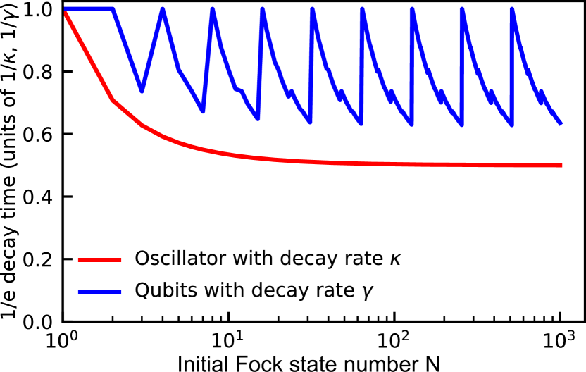
Figure 27: Effective decay time of $\braket{\hat{n}^{2}}$. We start from an initial Fock state with occupation $N$ and evolve under mode decay/qubit decay. Note that $\braket{\hat{n}}$ exhbits a decay time of $1/\kappa$, $1\gamma$, respectively, independent of $N$.

Notably, bosonic modes stored in high-Q cavities exhibit decay rates $\kappa$ that are roughly ten times lower than the decay rates $\gamma$ observed in typical qubits. Consequently, despite the fact that for $\kappa=\gamma$ the Fock-binary encoding results in the effective decay time of $\braket{\hat{n}^{2}}$ being up to twice as long, in reality, bosonic modes in cavities exhibit a significantly longer effective decay time for this observable.

References

- Di Meglio et al. [2024] A. Di Meglio, K. Jansen, I. Tavernelli, C. Alexandrou, S. Arunachalam, C. W. Bauer, K. Borras, S. Carrazza, A. Crippa, V. Croft, R. de Putter, A. Delgado, V. Dunjko, D. J. Egger, E. Fernández-Combarro, E. Fuchs, L. Funcke, D. González-Cuadra, M. Grossi, J. C. Halimeh, Z. Holmes, S. Kühn, D. Lacroix, R. Lewis, D. Lucchesi, M. L. Martinez, F. Meloni, A. Mezzacapo, S. Montangero, L. Nagano, V. R. Pascuzzi, V. Radescu, E. R. Ortega, A. Roggero, J. Schuhmacher, J. Seixas, P. Silvi, P. Spentzouris, F. Tacchino, K. Temme, K. Terashi, J. Tura, C. Tüysüz, S. Vallecorsa, U.-J. Wiese, S. Yoo, and J. Zhang, Quantum computing for high-energy physics: State of the art and challenges, PRX Quantum 5, 037001 (2024).
- Greiner et al. [2002] M. Greiner, O. Mandel, T. Esslinger, T. W. Hänsch, and I. Bloch, Quantum phase transition from a superfluid to a Mott insulator in a gas of ultracold atoms, Nature 415, 39 (2002).
- Blatt et al. [2013] R. Blatt, I. Bloch, I. Cirac, and P. Zoller, Quantum simulation - an exciting adventure, Ann. Phys. 525, A153 (2013).
- Georgescu et al. [2014] I. M. Georgescu, S. Ashhab, and F. Nori, Quantum simulation, Rev. Mod. Phys. 86, 153 (2014).
- Mazurenko et al. [2017] A. Mazurenko, C. S. Chiu, G. Ji, M. F. Parsons, M. Kanász-Nagy, R. Schmidt, F. Grusdt, E. Demler, D. Greif, and M. Greiner, A cold-atom Fermi-Hubbard antiferromagnet, Nature 545, 462 (2017).
- Semeghini et al. [2021] G. Semeghini, H. Levine, A. Keesling, S. Ebadi, T. T. Wang, D. Bluvstein, R. Verresen, H. Pichler, M. Kalinowski, R. Samajdar, A. Omran, S. Sachdev, A. Vishwanath, M. Greiner, V. Vuletić, and M. D. Lukin, Probing topological spin liquids on a programmable quantum simulator, Science 374, 1242 (2021).
- Shaw et al. [2024] A. L. Shaw, Z. Chen, J. Choi, D. K. Mark, P. Scholl, R. Finkelstein, A. Elben, S. Choi, and M. Endres, Benchmarking highly entangled states on a 60-atom analogue quantum simulator, Nature 628, 71 (2024).
- Brown et al. [2019] P. T. Brown, E. Guardado-Sanchez, B. M. Spar, E. W. Huang, T. P. Devereaux, and W. S. Bakr, Angle-resolved photoemission spectroscopy of a fermi–hubbard system, Nat. Phys. 16, 26–31 (2019).
- Joshi et al. [2022] M. K. Joshi, F. Kranzl, A. Schuckert, I. Lovas, C. Maier, R. Blatt, M. Knap, and C. F. Roos, Observing emergent hydrodynamics in a long-range quantum magnet, Science 376, 720–724 (2022).
- Wei et al. [2022] D. Wei, A. Rubio-Abadal, B. Ye, F. Machado, J. Kemp, K. Srakaew, S. Hollerith, J. Rui, S. Gopalakrishnan, N. Y. Yao, I. Bloch, and J. Zeiher, Quantum gas microscopy of kardar-parisi-zhang superdiffusion, Science 376, 716–720 (2022).
- Trotzky et al. [2012] S. Trotzky, Y.-A. Chen, A. Flesch, I. P. McCulloch, U. Schollwöck, J. Eisert, and I. Bloch, Probing the relaxation towards equilibrium in an isolated strongly correlated one-dimensional Bose gas, Nat. Phys. 8, 325 (2012).
- Schreiber et al. [2015] M. Schreiber, S. S. Hodgman, P. Bordia, H. P. Lüschen, M. H. Fischer, R. Vosk, E. Altman, U. Schneider, and I. Bloch, Observation of many-body localization of interacting fermions in a quasirandom optical lattice, Science 349, 842–845 (2015).
- Bernien et al. [2017] H. Bernien, S. Schwartz, A. Keesling, H. Levine, A. Omran, H. Pichler, S. Choi, A. S. Zibrov, M. Endres, M. Greiner, V. Vuletić, and M. D. Lukin, Probing many-body dynamics on a 51-atom quantum simulator, Nature 551, 579 (2017).
- Vivanco et al. [2023] F. J. Vivanco, A. Schuckert, S. Huang, G. L. Schumacher, G. G. T. Assumpção, Y. Ji, J. Chen, M. Knap, and N. Navon, The strongly driven fermi polaron (2023), arXiv:2308.05746 .
- Tagliacozzo et al. [2013] L. Tagliacozzo, A. Celi, P. Orland, M. W. Mitchell, and M. Lewenstein, Simulation of non-abelian gauge theories with optical lattices, Nat. Comm. 4, 1 (2013).
- Marcos et al. [2014] D. Marcos, P. Widmer, E. Rico, M. Hafezi, P. Rabl, U.-J. Wiese, and P. Zoller, Two-dimensional lattice gauge theories with superconducting quantum circuits, Ann. Phys. 351, 634 (2014).
- Zohar and Burrello [2015] E. Zohar and M. Burrello, Formulation of lattice gauge theories for quantum simulations, Phys. Rev. D 91, 054506 (2015).
- Kasper et al. [2017] V. Kasper, F. Hebenstreit, F. Jendrzejewski, M. K. Oberthaler, and J. Berges, Implementing quantum electrodynamics with ultracold atomic systems, New J. Phys. 19, 023030 (2017).
- Davoudi et al. [2021] Z. Davoudi, N. M. Linke, and G. Pagano, Toward simulating quantum field theories with controlled phonon-ion dynamics: A hybrid analog-digital approach, Phys. Rev. Res. 3, 043072 (2021).
- Aidelsburger et al. [2021] M. Aidelsburger, L. Barbiero, A. Bermudez, T. Chanda, A. Dauphin, D. González-Cuadra, P. R. Grzybowski, S. Hands, F. Jendrzejewski, J. Jünemann, G. Juzeliūnas, V. Kasper, A. Piga, S.-J. Ran, M. Rizzi, G. Sierra, L. Tagliacozzo, E. Tirrito, T. V. Zache, J. Zakrzewski, E. Zohar, and M. Lewenstein, Cold atoms meet lattice gauge theory, Phil. Trans. R. Soc. A 380 (2021).
- Andrade et al. [2022] B. Andrade, Z. Davoudi, T. Graß, M. Hafezi, G. Pagano, and A. Seif, Engineering an effective three-spin hamiltonian in trapped-ion systems for applications in quantum simulation, Quantum Sci. Technol. 7, 034001 (2022).
- Feldmeier et al. [2024] J. Feldmeier, N. Maskara, N. U. Köylüoğlu, and M. D. Lukin, Quantum simulation of dynamical gauge theories in periodically driven rydberg atom arrays (2024), arXiv:2408.02733 .
- Schweizer et al. [2019] C. Schweizer, F. Grusdt, M. Berngruber, L. Barbiero, E. Demler, N. Goldman, I. Bloch, and M. Aidelsburger, Floquet approach to z2 lattice gauge theories with ultracold atoms in optical lattices, Nat. Phys. 15, 1168 (2019).
- Mil et al. [2020] A. Mil, T. V. Zache, A. Hegde, A. Xia, R. P. Bhatt, M. K. Oberthaler, P. Hauke, J. Berges, and F. Jendrzejewski, A scalable realization of local u(1) gauge invariance in cold atomic mixtures, Science 367, 1128 (2020).
- Yang et al. [2020] B. Yang, H. Sun, R. Ott, H.-Y. Wang, T. V. Zache, J. C. Halimeh, Z.-S. Yuan, P. Hauke, and J.-W. Pan, Observation of gauge invariance in a 71-site bose–hubbard quantum simulator, Nature 587, 392 (2020).
- Zhou et al. [2022] Z.-Y. Zhou, G.-X. Su, J. C. Halimeh, R. Ott, H. Sun, P. Hauke, B. Yang, Z.-S. Yuan, J. Berges, and J.-W. Pan, Thermalization dynamics of a gauge theory on a quantum simulator, Science 377, 311 (2022).
- Martinez et al. [2016] E. A. Martinez, C. A. Muschik, P. Schindler, D. Nigg, A. Erhard, M. Heyl, P. Hauke, M. Dalmonte, T. Monz, P. Zoller, and R. Blatt, Real-time dynamics of lattice gauge theories with a few-qubit quantum computer, Nature 534, 516 (2016).
- Kokail et al. [2019] C. Kokail, C. Maier, R. van Bijnen, T. Brydges, M. K. Joshi, P. Jurcevic, C. A. Muschik, P. Silvi, R. Blatt, C. F. Roos, and P. Zoller, Self-verifying variational quantum simulation of lattice models, Nature 569, 355 (2019).
- Nguyen et al. [2022] N. H. Nguyen, M. C. Tran, Y. Zhu, A. M. Green, C. H. Alderete, Z. Davoudi, and N. M. Linke, Digital quantum simulation of the schwinger model and symmetry protection with trapped ions, PRX Quantum 3, 020324 (2022).
- Meth et al. [2023] M. Meth, J. F. Haase, J. Zhang, C. Edmunds, L. Postler, A. Steiner, A. J. Jena, L. Dellantonio, R. Blatt, P. Zoller, T. Monz, P. Schindler, C. Muschik, and M. Ringbauer, Simulating 2D lattice gauge theories on a qudit quantum computer (2023), arXiv:2310.12110 .
- Rad et al. [2024] A. Rad, A. Schuckert, E. Crane, G. Nambiar, F. Fei, J. Wyrick, R. M. Silver, M. Hafezi, Z. Davoudi, and M. J. Gullans, Analog quantum simulator of a quantum field theory with fermion-spin systems in silicon (2024), arXiv:2407.03419 .
- Bauer et al. [2023] C. W. Bauer, Z. Davoudi, N. Klco, and M. J. Savage, Quantum simulation of fundamental particles and forces, Nat. Rev. Phys. 5, 420 (2023).
- Ciavarella and Chernyshev [2022] A. N. Ciavarella and I. A. Chernyshev, Preparation of the su(3) lattice yang-mills vacuum with variational quantum methods, Phys. Rev. D 105, 074504 (2022).
- Ciavarella et al. [2021] A. Ciavarella, N. Klco, and M. J. Savage, Trailhead for quantum simulation of SU(3) Yang-Mills lattice gauge theory in the local multiplet basis, Phys. Rev. D 103, 094501 (2021).
- Klco et al. [2020] N. Klco, J. R. Stryker, and M. J. Savage, SU(2) non-Abelian gauge field theory in one dimension on digital quantum computers, Phys. Rev. D 101, 074512 (2020).
- Klco et al. [2018] N. Klco, E. F. Dumitrescu, A. J. McCaskey, T. D. Morris, R. C. Pooser, M. Sanz, E. Solano, P. Lougovski, and M. J. Savage, Quantum-classical computation of Schwinger model dynamics using quantum computers, Phys. Rev. A 98, 032331 (2018).
- de Jong et al. [2022] W. A. de Jong, K. Lee, J. Mulligan, M. Płoskoń, F. Ringer, and X. Yao, Quantum simulation of nonequilibrium dynamics and thermalization in the schwinger model, Phys. Rev. D 106, 054508 (2022).
- Mildenberger et al. [2022] J. Mildenberger, W. Mruczkiewicz, J. C. Halimeh, Z. Jiang, and P. Hauke, Probing confinement in a lattice gauge theory on a quantum computer (2022), arXiv:2203.08905 .
- Tudorovskaya and Muñoz Ramo [2024] M. Tudorovskaya and D. Muñoz Ramo, Quantum computing simulation of a mixed spin-boson hamiltonian and its performance for a cavity quantum electrodynamics problem, Phys. Rev. A 109, 032612 (2024).
- Farrell et al. [2024] R. C. Farrell, M. Illa, A. N. Ciavarella, and M. J. Savage, Quantum simulations of hadron dynamics in the schwinger model using 112 qubits, Phys. Rev. D 109, 114510 (2024).
- González-Cuadra et al. [2022] D. González-Cuadra, T. V. Zache, J. Carrasco, B. Kraus, and P. Zoller, Hardware efficient quantum simulation of non-abelian gauge theories with qudits on rydberg platforms, Phys. Rev. Lett. 129, 160501 (2022).
- Zache et al. [2023] T. V. Zache, D. González-Cuadra, and P. Zoller, Fermion-qudit quantum processors for simulating lattice gauge theories with matter, Quantum 7, 1140 (2023).
- Illa et al. [2024] M. Illa, C. E. P. Robin, and M. J. Savage, Qu8its for quantum simulations of lattice quantum chromodynamics, Phys. Rev. D 110, 014507 (2024).
- Sawaya et al. [2020] N. P. D. Sawaya, T. Menke, T. H. Kyaw, S. Johri, A. Aspuru-Guzik, and G. G. Guerreschi, Resource-efficient digital quantum simulation of d-level systems for photonic, vibrational, and spin-s hamiltonians, npj Quantum Inf. 6, 49 (2020).
- Liu et al. [2024a] Y. Liu, S. Singh, K. C. Smith, E. Crane, J. M. Martyn, A. Eickbusch, A. Schuckert, R. D. Li, J. Sinanan-Singh, M. B. Soley, T. Tsunoda, I. L. Chuang, N. Wiebe, and S. M. Girvin, Hybrid oscillator-qubit quantum processors: Instruction set architectures, abstract machine models, and applications, arXiv:2407.10381 (2024a).
- Zhang et al. [2023] J. Zhang, R. Ferguson, S. Kühn, J. F. Haase, C. Wilson, K. Jansen, and C. A. Muschik, Simulating gauge theories with variational quantum eigensolvers in superconducting microwave cavities, Quantum 7, 1148 (2023).
- Belyansky et al. [2024] R. Belyansky, S. Whitsitt, N. Mueller, A. Fahimniya, E. R. Bennewitz, Z. Davoudi, and A. V. Gorshkov, High-Energy Collision of Quarks and Mesons in the Schwinger Model: From Tensor Networks to Circuit QED, Phys. Rev. Lett. 132, 091903 (2024).
- Jha et al. [2024] R. G. Jha, F. Ringer, G. Siopsis, and S. Thompson, Continuous-variable quantum computation of the o(3) model in dimensions, Phys. Rev. A 109, 052412 (2024).
- Meekhof et al. [1996] D. M. Meekhof, C. Monroe, B. E. King, W. M. Itano, and D. J. Wineland, Generation of nonclassical motional states of a trapped atom, Phys. Rev. Lett. 76, 1796 (1996).
- Flühmann et al. [2019] C. Flühmann, T. L. Nguyen, M. Marinelli, V. Negnevitsky, K. Mehta, and J. P. Home, Encoding a qubit in a trapped-ion mechanical oscillator, Nature 566, 513 (2019).
- Liu et al. [2021] Y. Liu, J. Sinanan-Singh, M. T. Kearney, G. Mintzer, and I. L. Chuang, Constructing qudits from infinite-dimensional oscillators by coupling to qubits, Phys. Rev. A 104, 032605 (2021).
- Katz and Monroe [2023] O. Katz and C. Monroe, Programmable quantum simulations of bosonic systems with trapped ions, Phys. Rev. Lett. 131, 033604 (2023).
- Whitlow et al. [2023] J. Whitlow, Z. Jia, Y. Wang, C. Fang, J. Kim, and K. R. Brown, Quantum simulation of conical intersections using trapped ions, Nat. Chem. 15, 1509 (2023).
- Davoudi et al. [2020] Z. Davoudi, M. Hafezi, C. Monroe, G. Pagano, A. Seif, and A. Shaw, Towards analog quantum simulations of lattice gauge theories with trapped ions, Phys. Rev. Res. 2, 023015 (2020).
- Schlosser et al. [2001] N. Schlosser, G. Reymond, I. Protsenko, and P. Grangier, Sub-poissonian loading of single atoms in a microscopic dipole trap, Nature 411, 1024 (2001).
- Scholl et al. [2023] P. Scholl, A. L. Shaw, R. Finkelstein, R. B.-S. Tsai, J. Choi, and M. Endres, Erasure-cooling, control, and hyper-entanglement of motion in optical tweezers, arXiv:2311.15580 (2023).
- Martyn et al. [2021] J. M. Martyn, Z. M. Rossi, A. K. Tan, and I. L. Chuang, Grand unification of quantum algorithms, PRX Quantum 2, 040203 (2021).
- Wiese [2013] U.-J. Wiese, Ultracold quantum gases and lattice systems: quantum simulation of lattice gauge theories, Ann. Phys. 525, 777 (2013).
- Reagor et al. [2016] M. Reagor, W. Pfaff, C. Axline, R. W. Heeres, N. Ofek, K. Sliwa, E. Holland, C. Wang, J. Blumoff, K. Chou, M. J. Hatridge, L. Frunzio, M. H. Devoret, L. Jiang, and R. J. Schoelkopf, Quantum memory with millisecond coherence in circuit qed, Phys. Rev. B 94, 014506 (2016).
- Stavenger et al. [2022] T. J. Stavenger, E. Crane, K. C. Smith, C. T. Kang, S. M. Girvin, and N. Wiebe, C2QA - Bosonic Qiskit, in 2022 IEEE HPEC (2022) pp. 1–8.
- Wegner [1971] F. J. Wegner, Duality in generalized ising models and phase transitions without local order parameters, J. Math. Phys., J. Math. Phys. 12, 2259 (1971).
- Horn et al. [1979] D. Horn, M. Weinstein, and S. Yankielowicz, Hamiltonian approach to lattice gauge theories, Phys. Rev. D 19, 3715 (1979).
- Orland and Rohrlich [1990] P. Orland and D. Rohrlich, Lattice gauge magnets: Local isospin from spin, Nucl. Phys. B 338, 647 (1990).
- Chandrasekharan and Wiese [1997] S. Chandrasekharan and U. J. Wiese, Quantum link models: A Discrete approach to gauge theories, Nucl. Phys. B 492, 455 (1997).
- Mathur [2005] M. Mathur, Harmonic oscillator prepotentials in SU(2) lattice gauge theory, J. Phys. A 38, 10015 (2005).
- Zohar et al. [2013] E. Zohar, J. I. Cirac, and B. Reznik, Quantum simulations of gauge theories with ultracold atoms: local gauge invariance from angular momentum conservation, Phys. Rev. A 88, 023617 (2013).
- Mathur and Sreeraj [2015] M. Mathur and T. P. Sreeraj, Canonical transformations and loop formulation of su(n) lattice gauge theories, Phys. Rev. D 92, 125018 (2015).
- Gustafson [2021] E. Gustafson, Prospects for Simulating a Qudit Based Model of (1+1)d Scalar QED, Phys. Rev. D 103, 114505 (2021).
- Zache et al. [2022] T. V. Zache, M. Van Damme, J. C. Halimeh, P. Hauke, and D. Banerjee, Toward the continuum limit of a quantum link schwinger model, Phys. Rev. D 106, L091502 (2022).
- Coleman [1976] S. Coleman, More about the massive Schwinger model, Ann. Phys. 101, 239 (1976).
- Byrnes et al. [2002] T. M. R. Byrnes, P. Sriganesh, R. J. Bursill, and C. J. Hamer, Density matrix renormalization group approach to the massive Schwinger model, Phys. Rev. D 66, 013002 (2002).
- Buyens et al. [2017] B. Buyens, S. Montangero, J. Haegeman, F. Verstraete, and K. Van Acoleyen, Finite-representation approximation of lattice gauge theories at the continuum limit with tensor networks, Phys. Rev. D 95, 094509 (2017).
- Funcke et al. [2020] L. Funcke, K. Jansen, and S. Kühn, Topological vacuum structure of the Schwinger model with matrix product states, Phys. Rev. D 101, 054507 (2020).
- Wiese [2014] U.-J. Wiese, Towards quantum simulating QCD, Nucl. Phys. A 931, 246 (2014).
- Yang et al. [2016] D. Yang, G. S. Giri, M. Johanning, C. Wunderlich, P. Zoller, and P. Hauke, Analog quantum simulation of -dimensional lattice QED with trapped ions, Phys. Rev. A 94, 052321 (2016).
- Blais et al. [2004] A. Blais, R.-S. Huang, A. Wallraff, S. M. Girvin, and R. J. Schoelkopf, Cavity quantum electrodynamics for superconducting electrical circuits: An architecture for quantum computation, Phys. Rev. A 69, 062320 (2004).
- Milul et al. [2023] O. Milul, B. Guttel, U. Goldblatt, S. Hazanov, L. M. Joshi, D. Chausovsky, N. Kahn, E. Çiftyürek, F. Lafont, and S. Rosenblum, Superconducting cavity qubit with tens of milliseconds single-photon coherence time, PRX Quantum 4, 030336 (2023).
- Romanenko et al. [2020] A. Romanenko, R. Pilipenko, S. Zorzetti, D. Frolov, M. Awida, S. Belomestnykh, S. Posen, and A. Grassellino, Three-dimensional superconducting resonators at mk with photon lifetimes up to s, Phys. Rev. Appl. 13, 034032 (2020).
- Ganjam et al. [2024] S. Ganjam, Y. Wang, Y. Lu, A. Banerjee, C. U. Lei, L. Krayzman, K. Kisslinger, C. Zhou, R. Li, Y. Jia, M. Liu, L. Frunzio, and R. J. Schoelkopf, Surpassing millisecond coherence in on chip superconducting quantum memories by optimizing materials and circuit design, Nat. Comm. 15, 3687 (2024).
- Chakram et al. [2021] S. Chakram, A. E. Oriani, R. K. Naik, A. V. Dixit, K. He, A. Agrawal, H. Kwon, and D. I. Schuster, Seamless high- microwave cavities for multimode circuit quantum electrodynamics, Phys. Rev. Lett. 127, 107701 (2021).
- Blais et al. [2021] A. Blais, A. L. Grimsmo, S. M. Girvin, and A. Wallraff, Circuit quantum electrodynamics, Rev. Mod. Phys. 93, 025005 (2021).
- Koch et al. [2007] J. Koch, T. M. Yu, J. Gambetta, A. A. Houck, D. I. Schuster, J. Majer, A. Blais, M. H. Devoret, S. M. Girvin, and R. J. Schoelkopf, Charge-insensitive qubit design derived from the cooper pair box, Phys. Rev. A 76, 042319 (2007).
- Schreier et al. [2008] J. A. Schreier, A. A. Houck, J. Koch, D. I. Schuster, B. R. Johnson, J. M. Chow, J. M. Gambetta, J. Majer, L. Frunzio, M. H. Devoret, S. M. Girvin, and R. J. Schoelkopf, Suppressing charge noise decoherence in superconducting charge qubits, Phys. Rev. B 77, 180502 (2008).
- Sivak et al. [2023] V. V. Sivak, A. Eickbusch, B. Royer, S. Singh, I. Tsioutsios, S. Ganjam, A. Miano, B. L. Brock, A. Z. Ding, L. Frunzio, S. M. Girvin, R. J. Schoelkopf, and M. H. Devoret, Real-time quantum error correction beyond break-even, Nature 616, 50 (2023).
- Wang et al. [2022] C. Wang, X. Li, H. Xu, Z. Li, J. Wang, Z. Yang, Z. Mi, X. Liang, T. Su, C. Yang, G. Wang, W. Wang, Y. Li, M. Chen, C. Li, K. Linghu, J. Han, Y. Zhang, Y. Feng, Y. Song, T. Ma, J. Zhang, R. Wang, P. Zhao, W. Liu, G. Xue, Y. Jin, and H. Yu, Towards practical quantum computers: transmon qubit with a lifetime approaching 0.5 milliseconds, npj Quantum Inf. 8, 3 (2022).
- Chapman et al. [2023] B. J. Chapman, S. J. de Graaf, S. H. Xue, Y. Zhang, J. Teoh, J. C. Curtis, T. Tsunoda, A. Eickbusch, A. P. Read, A. Koottandavida, S. O. Mundhada, L. Frunzio, M. Devoret, S. Girvin, and R. Schoelkopf, High-on-off-ratio beam-splitter interaction for gates on bosonically encoded qubits, PRX Quantum 4, 020355 (2023).
- Sivak et al. [2019] V. Sivak, N. Frattini, V. Joshi, A. Lingenfelter, S. Shankar, and M. Devoret, Kerr-free three-wave mixing in superconducting quantum circuits, Phys. Rev. Appl. 11, 054060 (2019).
- Chien et al. [2020] T.-C. Chien, O. Lanes, C. Liu, X. Cao, P. Lu, S. Motz, G. Liu, D. Pekker, and M. Hatridge, Multiparametric amplification and qubit measurement with a kerr-free josephson ring modulator, Phys. Rev. A 101, 042336 (2020).
- Eickbusch et al. [2022] A. Eickbusch, V. Sivak, A. Z. Ding, S. S. Elder, S. R. Jha, J. Venkatraman, B. Royer, S. M. Girvin, R. J. Schoelkopf, and M. H. Devoret, Fast universal control of an oscillator with weak dispersive coupling to a qubit, Nat. Phys. 18, 1464 (2022).
- Heeres et al. [2015] R. W. Heeres, B. Vlastakis, E. Holland, S. Krastanov, V. V. Albert, L. Frunzio, L. Jiang, and R. J. Schoelkopf, Cavity state manipulation using photon-number selective phase gates, Phys. Rev. Lett. 115, 137002 (2015).
- Chou et al. [2024] K. S. Chou, T. Shemma, H. McCarrick, T.-C. Chien, J. D. Teoh, P. Winkel, A. Anderson, J. Chen, J. C. Curtis, S. J. de Graaf, J. W. O. Garmon, B. Gudlewski, W. D. Kalfus, T. Keen, N. Khedkar, C. U. Lei, G. Liu, P. Lu, Y. Lu, A. Maiti, L. Mastalli-Kelly, N. Mehta, S. O. Mundhada, A. Narla, T. Noh, T. Tsunoda, S. H. Xue, J. O. Yuan, L. Frunzio, J. Aumentado, S. Puri, S. M. Girvin, S. H. Moseley, and R. J. Schoelkopf, A superconducting dual-rail cavity qubit with erasure-detected logical measurements, Nat. Phys. 0, 0 (2024).
- Burkhart et al. [2021a] L. D. Burkhart, J. D. Teoh, Y. Zhang, C. J. Axline, L. Frunzio, M. Devoret, L. Jiang, S. Girvin, and R. Schoelkopf, Error-detected state transfer and entanglement in a superconducting quantum network, PRX Quantum 2, 030321 (2021a).
- Elder et al. [2020] S. S. Elder, C. S. Wang, P. Reinhold, C. T. Hann, K. S. Chou, B. J. Lester, S. Rosenblum, L. Frunzio, L. Jiang, and R. J. Schoelkopf, High-fidelity measurement of qubits encoded in multilevel superconducting circuits, Phys. Rev. X 10, 011001 (2020).
- Tsunoda et al. [2023a] T. Tsunoda, J. D. Teoh, W. D. Kalfus, S. J. de Graaf, B. J. Chapman, J. C. Curtis, N. Thakur, S. M. Girvin, and R. J. Schoelkopf, Error-detectable bosonic entangling gates with a noisy ancilla, PRX Quantum 4, 020354 (2023a).
- Curtis et al. [2021] J. C. Curtis, C. T. Hann, S. S. Elder, C. S. Wang, L. Frunzio, L. Jiang, and R. J. Schoelkopf, Single-shot number-resolved detection of microwave photons with error mitigation, Phys. Rev. A 103, 023705 (2021).
- Wang et al. [2023] C. S. Wang, N. E. Frattini, B. J. Chapman, S. Puri, S. M. Girvin, M. H. Devoret, and R. J. Schoelkopf, Observation of wave-packet branching through an engineered conical intersection, Phys. Rev. X 13, 011008 (2023).
- Kubica et al. [2023] A. Kubica, A. Haim, Y. Vaknin, H. Levine, F. Brandão, and A. Retzker, Erasure qubits: Overcoming the limit in superconducting circuits, Phys. Rev. X 13, 041022 (2023).
- Teoh et al. [2023] J. D. Teoh, P. Winkel, H. K. Babla, B. J. Chapman, J. Claes, S. J. de Graaf, J. W. O. Garmon, W. D. Kalfus, Y. Lu, A. Maiti, K. Sahay, N. Thakur, T. Tsunoda, S. H. Xue, L. Frunzio, S. M. Girvin, S. Puri, and R. J. Schoelkopf, Dual-rail encoding with superconducting cavities, PNAS 120, e2221736120 (2023).
- Levine et al. [2024] H. Levine, A. Haim, J. S. C. Hung, N. Alidoust, M. Kalaee, L. DeLorenzo, E. A. Wollack, P. Arrangoiz-Arriola, A. Khalajhedayati, R. Sanil, H. Moradinejad, Y. Vaknin, A. Kubica, D. Hover, S. Aghaeimeibodi, J. A. Alcid, C. Baek, J. Barnett, K. Bawdekar, P. Bienias, H. A. Carson, C. Chen, L. Chen, H. Chinkezian, E. M. Chisholm, A. Clifford, R. Cosmic, N. Crisosto, A. M. Dalzell, E. Davis, J. M. D’Ewart, S. Diez, N. D’Souza, P. T. Dumitrescu, E. Elkhouly, M. T. Fang, Y. Fang, S. Flammia, M. J. Fling, G. Garcia, M. K. Gharzai, A. V. Gorshkov, M. J. Gray, S. Grimberg, A. L. Grimsmo, C. T. Hann, Y. He, S. Heidel, S. Howell, M. Hunt, J. Iverson, I. Jarrige, L. Jiang, W. M. Jones, R. Karabalin, P. J. Karalekas, A. J. Keller, D. Lasi, M. Lee, V. Ly, G. MacCabe, N. Mahuli, G. Marcaud, M. H. Matheny, S. McArdle, G. McCabe, G. Merton, C. Miles, A. Milsted, A. Mishra, L. Moncelsi, M. Naghiloo, K. Noh, E. Oblepias, G. Ortuno, J. C. Owens, J. Pagdilao, A. Panduro, J.-P. Paquette, R. N. Patel, G. Peairs, D. J. Perello, E. C. Peterson, S. Ponte, H. Putterman, G. Refael, P. Reinhold, R. Resnick, O. A. Reyna, R. Rodriguez, J. Rose, A. H. Rubin, M. Runyan, C. A. Ryan, A. Sahmoud, T. Scaffidi, B. Shah, S. Siavoshi, P. Sivarajah, T. Skogland, C.-J. Su, L. J. Swenson, J. Sylvia, S. M. Teo, A. Tomada, G. Torlai, M. Wistrom, K. Zhang, I. Zuk, A. A. Clerk, F. G. S. L. Brandão, A. Retzker, and O. Painter, Demonstrating a long-coherence dual-rail erasure qubit using tunable transmons, Phys. Rev. X 14, 011051 (2024).
- Tsunoda et al. [2023b] T. Tsunoda, J. D. Teoh, W. D. Kalfus, S. J. de Graaf, B. J. Chapman, J. C. Curtis, N. Thakur, S. M. Girvin, and R. J. Schoelkopf, Error-detectable bosonic entangling gates with a noisy ancilla, PRX Quantum 4, 020354 (2023b).
- Koottandavida et al. [2023] A. Koottandavida, I. Tsioutsios, A. Kargioti, C. R. Smith, V. R. Joshi, W. Dai, J. D. Teoh, J. C. Curtis, L. Frunzio, R. J. Schoelkopf, and M. H. Devoret, Erasure detection of a dual-rail qubit encoded in a double-post superconducting cavity (2023), arXiv:2311.04423 .
- Kang et al. [2023] C. Kang, M. B. Soley, E. Crane, S. M. Girvin, and N. Wiebe, Leveraging Hamiltonian Simulation Techniques to Compile Operations on Bosonic Devices (2023), arXiv:2303.15542 .
- Lu et al. [2023] Y. Lu, A. Maiti, J. W. O. Garmon, S. Ganjam, Y. Zhang, J. Claes, L. Frunzio, S. M. Girvin, and R. J. Schoelkopf, High-fidelity parametric beamsplitting with a parity-protected converter, Nat. Comm. 14, 5767 (2023).
- Sørensen and Mølmer [1999] A. Sørensen and K. Mølmer, Quantum computation with ions in thermal motion, Phys. Rev. Lett. 82, 1971 (1999).
- Mølmer and Sørensen [1999] K. Mølmer and A. Sørensen, Multiparticle entanglement of hot trapped ions, Phys. Rev. Lett. 82, 1835 (1999).
- Stoneham et al. [2003] A. M. Stoneham, A. J. Fisher, and P. T. Greenland, Optically driven silicon-based quantum gates with potential for high-temperature operation, J. Phys.: Condens. Matter 15, L447 (2003).
- Crane et al. [2019] E. Crane, T. Crane, A. Schuckert, N. H. Le, K. Stockbridge, S. Chick, and A. J. Fisher, Optically controlled entangling gates in randomly doped silicon, Phys. Rev. B 100, 064201 (2019).
- Crane et al. [2021] E. Crane, A. Schuckert, N. H. Le, and A. J. Fisher, Rydberg entangling gates in silicon, Phys. Rev. Res. 3, 033086 (2021).
- Katz et al. [2023a] O. Katz, M. Cetina, and C. Monroe, Programmable -body interactions with trapped ions, PRX Quantum 4, 030311 (2023a).
- Katz et al. [2023b] O. Katz, L. Feng, A. Risinger, C. Monroe, and M. Cetina, Demonstration of three- and four-body interactions between trapped-ion spins, Nat. Phys. 19, 1452–1458 (2023b).
- Peierls [1933] R. Peierls, Zur theorie des diamagnetismus von leitungselektronen, Zeitschrift für Physik 80, 763–791 (1933).
- Girvin [2005] S. M. Girvin, Introduction to the fractional quantum hall effect, in The Quantum Hall Effect (Birkhäuser Basel, 2005) p. 133–162.
- Kivlichan et al. [2018] I. D. Kivlichan, J. McClean, N. Wiebe, C. Gidney, A. Aspuru-Guzik, G. K.-L. Chan, and R. Babbush, Quantum simulation of electronic structure with linear depth and connectivity, Phys. Rev. Lett. 120, 110501 (2018).
- Foxen et al. [2020] B. Foxen, C. Neill, A. Dunsworth, P. Roushan, B. Chiaro, A. Megrant, J. Kelly, Z. Chen, K. Satzinger, R. Barends, F. Arute, K. Arya, R. Babbush, D. Bacon, J. C. Bardin, S. Boixo, D. Buell, B. Burkett, Y. Chen, R. Collins, E. Farhi, A. Fowler, C. Gidney, M. Giustina, R. Graff, M. Harrigan, T. Huang, S. V. Isakov, E. Jeffrey, Z. Jiang, D. Kafri, K. Kechedzhi, P. Klimov, A. Korotkov, F. Kostritsa, D. Landhuis, E. Lucero, J. McClean, M. McEwen, X. Mi, M. Mohseni, J. Y. Mutus, O. Naaman, M. Neeley, M. Niu, A. Petukhov, C. Quintana, N. Rubin, D. Sank, V. Smelyanskiy, A. Vainsencher, T. C. White, Z. Yao, P. Yeh, A. Zalcman, H. Neven, and J. M. Martinis (Google AI Quantum), Demonstrating a continuous set of two-qubit gates for near-term quantum algorithms, Phys. Rev. Lett. 125, 120504 (2020).
- Moses et al. [2023] S. A. Moses, C. H. Baldwin, M. S. Allman, R. Ancona, L. Ascarrunz, C. Barnes, J. Bartolotta, B. Bjork, P. Blanchard, M. Bohn, J. G. Bohnet, N. C. Brown, N. Q. Burdick, W. C. Burton, S. L. Campbell, J. P. Campora, C. Carron, J. Chambers, J. W. Chan, Y. H. Chen, A. Chernoguzov, E. Chertkov, J. Colina, J. P. Curtis, R. Daniel, M. DeCross, D. Deen, C. Delaney, J. M. Dreiling, C. T. Ertsgaard, J. Esposito, B. Estey, M. Fabrikant, C. Figgatt, C. Foltz, M. Foss-Feig, D. Francois, J. P. Gaebler, T. M. Gatterman, C. N. Gilbreth, J. Giles, E. Glynn, A. Hall, A. M. Hankin, A. Hansen, D. Hayes, B. Higashi, I. M. Hoffman, B. Horning, J. J. Hout, R. Jacobs, J. Johansen, L. Jones, J. Karcz, T. Klein, P. Lauria, P. Lee, D. Liefer, S. T. Lu, D. Lucchetti, C. Lytle, A. Malm, M. Matheny, B. Mathewson, K. Mayer, D. B. Miller, M. Mills, B. Neyenhuis, L. Nugent, S. Olson, J. Parks, G. N. Price, Z. Price, M. Pugh, A. Ransford, A. P. Reed, C. Roman, M. Rowe, C. Ryan-Anderson, S. Sanders, J. Sedlacek, P. Shevchuk, P. Siegfried, T. Skripka, B. Spaun, R. T. Sprenkle, R. P. Stutz, M. Swallows, R. I. Tobey, A. Tran, T. Tran, E. Vogt, C. Volin, J. Walker, A. M. Zolot, and J. M. Pino, A race-track trapped-ion quantum processor, Phys. Rev. X 13, 041052 (2023).
- Hémery et al. [2024] K. Hémery, K. Ghanem, E. Crane, S. L. Campbell, J. M. Dreiling, C. Figgatt, C. Foltz, J. P. Gaebler, J. Johansen, M. Mills, S. A. Moses, J. M. Pino, A. Ransford, M. Rowe, P. Siegfried, R. P. Stutz, H. Dreyer, A. Schuckert, and R. Nigmatullin, Measuring the Loschmidt Amplitude for Finite-Energy Properties of the Fermi-Hubbard Model on an Ion-Trap Quantum Computer, PRX Quantum 5, 030323 (2024).
- Holstein [1959] T. Holstein, Studies of polaron motion, Ann. Phys. 8, 325–342 (1959).
- Knörzer et al. [2022] J. Knörzer, T. Shi, E. Demler, and J. I. Cirac, Spin-holstein models in trapped-ion systems, Phys. Rev. Lett. 128, 120404 (2022).
- Li et al. [2020] J. Li, D. Golez, G. Mazza, A. J. Millis, A. Georges, and M. Eckstein, Electromagnetic coupling in tight-binding models for strongly correlated light and matter, Phys. Rev. B 101, 205140 (2020).
- Childs and Wiebe [2013] A. M. Childs and N. Wiebe, Product formulas for exponentials of commutators, J. Math. Phys. 54, 6 (2013).
- Childs et al. [2021] A. M. Childs, Y. Su, M. C. Tran, N. Wiebe, and S. Zhu, Theory of trotter error with commutator scaling, Phys. Rev. X 11, 011020 (2021).
- Shaw et al. [2020] A. F. Shaw, P. Lougovski, J. R. Stryker, and N. Wiebe, Quantum algorithms for simulating the lattice schwinger model, Quantum 4, 306 (2020).
- Rhodes et al. [2024] M. Rhodes, M. Kreshchuk, and S. Pathak, Exponential improvements in the simulation of lattice gauge theories using near-optimal techniques (2024), arXiv:2405.10416 .
- Roth [2006] R. Roth, Introduction to Coding Theory (Cambridge University Press, 2006).
- Jordan et al. [2012] S. P. Jordan, K. S. M. Lee, and J. Preskill, Quantum Algorithms for Quantum Field Theories, Science 336, 1130 (2012).
- Veis et al. [2016] L. Veis, J. Višňák, H. Nishizawa, H. Nakai, and J. Pittner, Quantum chemistry beyond born–oppenheimer approximation on a quantum computer: A simulated phase estimation study, Int. J. Quantum Chem. 116, 1328 (2016).
- Tong et al. [2022] Y. Tong, V. V. Albert, J. R. McClean, J. Preskill, and Y. Su, Provably accurate simulation of gauge theories and bosonic systems, Quantum 6, 816 (2022).
- Häner et al. [2018] T. Häner, M. Roetteler, and K. M. Svore, Optimizing quantum circuits for arithmetic, arXiv preprint arXiv:1805.12445 (2018).
- Low and Chuang [2017a] G. H. Low and I. L. Chuang, Hamiltonian simulation by uniform spectral amplification (2017a), arXiv:1707.05391 .
- Low and Wiebe [2018] G. H. Low and N. Wiebe, Hamiltonian simulation in the interaction picture (2018), arXiv:1805.00675 .
- Javadi-Abhari et al. [2024] A. Javadi-Abhari, M. Treinish, K. Krsulich, C. J. Wood, J. Lishman, J. Gacon, S. Martiel, P. D. Nation, L. S. Bishop, A. W. Cross, B. R. Johnson, and J. M. Gambetta, Quantum computing with Qiskit (2024), arXiv:2405.08810 .
- Kebric et al. [2021] M. Kebric, L. Barbiero, C. Reinmoser, U. Schollwöck, and F. Grusdt, Confinement and mott transitions of dynamical charges in one-dimensional lattice gauge theories, Phys. Rev. Lett. 127, 167203 (2021).
- Kitaev [2003] A. Kitaev, Fault-tolerant quantum computation by anyons, Ann. Phys. 303, 2 (2003).
- Homeier et al. [2021] L. Homeier, C. Schweizer, M. Aidelsburger, A. Fedorov, and F. Grusdt, Z2 lattice gauge theories and kitaev’s toric code: A scheme for analog quantum simulation, Phys. Rev. B 104, 085138 (2021).
- Barbiero et al. [2019] L. Barbiero, C. Schweizer, M. Aidelsburger, E. Demler, N. Goldman, and F. Grusdt, Coupling ultracold matter to dynamical gauge fields in optical lattices: From flux attachment to lattice gauge theories, Sci. Adv. 5 (2019).
- Borla et al. [2020] U. Borla, R. Verresen, F. Grusdt, and S. Moroz, Confined phases of one-dimensional spinless fermions coupled to Z2 gauge theory, Phys. Rev. Lett. 124 (2020).
- Schuckert et al. [2024] A. Schuckert et al., Constrained phases in a -Higgs model , in preparation (2024).
- Coleman et al. [1975] S. Coleman, R. Jackiw, and L. Susskind, Charge shielding and quark confinement in the massive schwinger model, Ann. Phys. 93, 267 (1975).
- Angelides et al. [2023a] T. Angelides, L. Funcke, K. Jansen, and S. Kühn, Computing the mass shift of Wilson and staggered fermions in the lattice Schwinger model with matrix product states, Phys. Rev. D 108, 014516 (2023a).
- Funcke et al. [2023] L. Funcke, K. Jansen, and S. Kühn, Exploring the -violating dashen phase in the schwinger model with tensor networks, Phys. Rev. D 108, 014504 (2023).
- Bañuls et al. [2018] M. C. Bañuls, K. Cichy, J. I. Cirac, K. Jansen, and S. Kühn, Tensor Networks and their use for Lattice Gauge Theories, Proc. Sci., LATTICE2018 334, (2018).
- Angelides et al. [2023b] T. Angelides, P. Naredi, A. Crippa, K. Jansen, S. Kühn, I. Tavernelli, and D. S. Wang, First-order phase transition of the schwinger model with a quantum computer (2023b), arXiv:2312.12831 .
- Schuch et al. [2008] N. Schuch, M. M. Wolf, F. Verstraete, and J. I. Cirac, Entropy Scaling and Simulability by Matrix Product States, Phys. Rev. Lett. 100, 030504 (2008).
- Rodriguez-Nieva et al. [2022] J. F. Rodriguez-Nieva, A. Schuckert, D. Sels, M. Knap, and E. Demler, Transverse instability and universal decay of spin spiral order in the heisenberg model, Phys. Rev. B 105, L060302 (2022).
- Schollwöck [2011] U. Schollwöck, The density-matrix renormalization group in the age of matrix product states, Ann. Phys. 326, 96 (2011).
- Orús [2014] R. Orús, A practical introduction to tensor networks: Matrix product states and projected entangled pair states, Ann. Phys. 349, 117 (2014).
- Bridgeman and Chubb [2017] J. C. Bridgeman and C. T. Chubb, Hand-waving and interpretive dance: an introductory course on tensor networks, J. Phys. A: Math. Theor. 50, 223001 (2017).
- Verstraete and Cirac [2004] F. Verstraete and J. I. Cirac, Renormalization algorithms for Quantum-Many Body Systems in two and higher dimensions, arXiv:cond-mat/0407066 (2004).
- Lubasch et al. [2014] M. Lubasch, J. I. Cirac, and M.-C. Bañuls, Algorithms for finite projected entangled pair states, Phys. Rev. B 90, 064425 (2014).
- Kuramashi and Yoshimura [2019] Y. Kuramashi and Y. Yoshimura, Three-dimensional finite temperature z2 gauge theory with tensor network scheme, J. High Energ. Phys. 2019 (8), 23.
- Felser et al. [2020] T. Felser, P. Silvi, M. Collura, and S. Montangero, Two-dimensional quantum-link lattice Quantum Electrodynamics at finite density, Phys. Rev. X 10, 041040 (2020).
- Magnifico et al. [2021] G. Magnifico, T. Felser, P. Silvi, and S. Montangero, Lattice quantum electrodynamics in (3+1)-dimensions at finite density with tensor networks, Nat. Comm. 12, 3600 (2021).
- Kühn et al. [2014] S. Kühn, J. I. Cirac, and M.-C. Bañuls, Quantum simulation of the Schwinger model: A study of feasibility, Phys. Rev. A 90, 042305 (2014).
- Bǎzǎvan et al. [2024] O. Bǎzǎvan, S. Saner, E. Tirrito, G. Araneda, R. Srinivas, and A. Bermudez, Synthetic gauge theories based on parametric excitations of trapped ions, Comm. Phys. 7, 229 (2024).
- Smith et al. [2023] K. C. Smith, E. Crane, T. Stavenger, and S. Girvin, Introducing Bosonic Qiskit: A package for simulating bosonic and hybrid qubit-bosonic circuits, Qiskit Blog (2023).
- Peruzzo et al. [2014] A. Peruzzo, J. McClean, P. Shadbolt, M.-H. Yung, X.-Q. Zhou, P. J. Love, A. Aspuru-Guzik, and J. L. O’Brien, A variational eigenvalue solver on a photonic quantum processor, Nat. Comm. 5 (2014).
- Farhi et al. [2014] E. Farhi, J. Goldstone, and S. Gutmann, A quantum approximate optimization algorithm (2014), arXiv:1411.4028 .
- McClean et al. [2016] J. R. McClean, J. Romero, R. Babbush, and A. Aspuru-Guzik, The theory of variational hybrid quantum-classical algorithms, New J. Phys. 18, 023023 (2016).
- McClean et al. [2018] J. R. McClean, S. Boixo, V. N. Smelyanskiy, R. Babbush, and H. Neven, Barren plateaus in quantum neural network training landscapes, Nat. Comm. 9 (2018).
- Grimsley et al. [2019] H. R. Grimsley, S. E. Economou, E. Barnes, and N. J. Mayhall, An adaptive variational algorithm for exact molecular simulations on a quantum computer, Nat. Comm. 10 (2019).
- Wang et al. [2021] S. Wang, E. Fontana, M. Cerezo, K. Sharma, A. Sone, L. Cincio, and P. J. Coles, Noise-induced barren plateaus in variational quantum algorithms, Nat. Comm. 12 (2021).
- Yalouz et al. [2021] S. Yalouz, B. Senjean, F. Miatto, and V. Dunjko, Encoding strongly-correlated many-boson wavefunctions on a photonic quantum computer: application to the attractive bose-hubbard model, Quantum 5, 572 (2021).
- Mei et al. [2022] Q.-X. Mei, B.-W. Li, Y.-K. Wu, M.-L. Cai, Y. Wang, L. Yao, Z.-C. Zhou, and L.-M. Duan, Experimental realization of the rabi-hubbard model with trapped ions, Phys. Rev. Lett. 128, 160504 (2022).
- Zhang and Zhuang [2023] B. Zhang and Q. Zhuang, Energy-dependent barren plateau in bosonic variational quantum circuits (2023), arXiv:2305.01799 .
- Hadfield et al. [2019] S. Hadfield, Z. Wang, B. O’Gorman, E. Rieffel, D. Venturelli, and R. Biswas, From the quantum approximate optimization algorithm to a quantum alternating operator ansatz, Algorithms 12, 34 (2019).
- Saleem et al. [2023] Z. H. Saleem, T. Tomesh, B. Tariq, and M. Suchara, Approaches to constrained quantum approximate optimization, SN Comput. Sci. 4 (2023).
- Fontana et al. [2021] E. Fontana, N. Fitzpatrick, D. M. n. Ramo, R. Duncan, and I. Rungger, Evaluating the noise resilience of variational quantum algorithms, Phys. Rev. A 104, 022403 (2021).
- Wang et al. [2020] C. S. Wang, J. C. Curtis, B. J. Lester, Y. Zhang, Y. Y. Gao, J. Freeze, V. S. Batista, P. H. Vaccaro, I. L. Chuang, L. Frunzio, L. Jiang, S. M. Girvin, and R. J. Schoelkopf, Efficient multiphoton sampling of molecular vibronic spectra on a superconducting bosonic processor, Phys. Rev. X 10, 021060 (2020).
- Ofek et al. [2016] N. Ofek, A. Petrenko, R. Heeres, P. Reinhold, Z. Leghtas, B. Vlastakis, Y. Liu, L. Frunzio, S. M. Girvin, L. Jiang, M. Mirrahimi, M. H. Devoret, and R. J. Schoelkopf, Extending the lifetime of a quantum bit with error correction in superconducting circuits, Nature 536, 441–445 (2016).
- Spall [1998a] J. C. Spall, An overview of the simultaneous perturbation method for efficient optimization, Johns Hopkins APL Technical Digest 19, 482 (1998a).
- Spall [1998b] J. Spall, Implementation of the simultaneous perturbation algorithm for stochastic optimization, IEEE Trans. Aerosp. Electron. Syst. 34, 817 (1998b).
- Polyak [1990] B. Polyak, New stochastic approximation type procedures, Avtomatica i Telemekhanika 7, 98 (1990).
- Polyak and Juditsky [1992] B. T. Polyak and A. B. Juditsky, Acceleration of stochastic approximation by averaging, SIAM J. Control Optim. 30, 838–855 (1992).
- Kübler et al. [2020] J. M. Kübler, A. Arrasmith, L. Cincio, and P. J. Coles, An Adaptive Optimizer for Measurement-Frugal Variational Algorithms, Quantum 4, 263 (2020).
- Arrasmith et al. [2020] A. Arrasmith, L. Cincio, R. D. Somma, and P. J. Coles, Operator sampling for shot-frugal optimization in variational algorithms (2020), arXiv:2004.06252 .
- Gu et al. [2021] A. Gu, A. Lowe, P. A. Dub, P. J. Coles, and A. Arrasmith, Adaptive shot allocation for fast convergence in variational quantum algorithms (2021), arXiv:2108.10434 .
- Scriva et al. [2024] G. Scriva, N. Astrakhantsev, S. Pilati, and G. Mazzola, Challenges of variational quantum optimization with measurement shot noise, Phys. Rev. A 109, 032408 (2024).
- Barenco et al. [1997] A. Barenco, A. Berthiaume, D. Deutsch, A. Ekert, R. Jozsa, and C. Macchiavello, Stabilization of quantum computations by symmetrization, SIAM J. Comput. 26, 1541 (1997).
- Buhrman et al. [2001] H. Buhrman, R. Cleve, J. Watrous, and R. de Wolf, Quantum fingerprinting, Phys. Rev. Lett. 87, 167902 (2001).
- Filip [2002] R. Filip, Overlap and entanglement-witness measurements, Phys. Rev. A 65, 062320 (2002).
- Aharonov et al. [2008] D. Aharonov, V. Jones, and Z. Landau, A polynomial quantum algorithm for approximating the jones polynomial, Algorithmica 55, 395–421 (2008).
- Iqbal et al. [2024] M. Iqbal, N. Tantivasadakarn, T. M. Gatterman, J. A. Gerber, K. Gilmore, D. Gresh, A. Hankin, N. Hewitt, C. V. Horst, M. Matheny, T. Mengle, B. Neyenhuis, A. Vishwanath, M. Foss-Feig, R. Verresen, and H. Dreyer, Topological order from measurements and feed-forward on a trapped ion quantum computer, Comm. Phys. 7, 1 (2024).
- Rajput et al. [2022] A. Rajput, A. Roggero, and N. Wiebe, Quantum error correction with gauge symmetries (2022), arXiv:2112.05186 .
- Temme et al. [2017] K. Temme, S. Bravyi, and J. M. Gambetta, Error mitigation for short-depth quantum circuits, Phys. Rev. Lett. 119, 180509 (2017).
- Li and Benjamin [2017] Y. Li and S. C. Benjamin, Efficient variational quantum simulator incorporating active error minimization, Phys. Rev. X 7, 021050 (2017).
- Halimeh and Hauke [2020] J. C. Halimeh and P. Hauke, Reliability of lattice gauge theories, Phys. Rev. Lett. 125, 030503 (2020).
- Halimeh et al. [2022] J. C. Halimeh, L. Homeier, C. Schweizer, M. Aidelsburger, P. Hauke, and F. Grusdt, Stabilizing lattice gauge theories through simplified local pseudogenerators, Phys. Rev. Res. 4, 033120 (2022).
- Halimeh et al. [2021] J. C. Halimeh, H. Lang, J. Mildenberger, Z. Jiang, and P. Hauke, Gauge-symmetry protection using single-body terms, PRX Quantum 2, 040311 (2021).
- Gilyén et al. [2019] A. Gilyén, Y. Su, G. H. Low, and N. Wiebe, Quantum singular value transformation and beyond: exponential improvements for quantum matrix arithmetics, in Proceedings of the 51st Annual ACM SIGACT Symposium on Theory of Computing (ACM, 2019).
- Kiely and Mueller [2022] T. G. Kiely and E. J. Mueller, Superfluidity in the one-dimensional bose-hubbard model, Phys. Rev. B 105, 134502 (2022).
- Prokof’ev and Svistunov [2000] N. V. Prokof’ev and B. V. Svistunov, Two definitions of superfluid density, Phys. Rev. B 61, 11282 (2000).
- Mari et al. [2021] A. Mari, T. R. Bromley, and N. Killoran, Estimating the gradient and higher-order derivatives on quantum hardware, Phys. Rev. A 103, 012405 (2021).
- Low and Chuang [2017b] G. H. Low and I. L. Chuang, Optimal hamiltonian simulation by quantum signal processing, Phys. Rev. Lett. 118, 010501 (2017b).
- Low and Chuang [2019] G. H. Low and I. L. Chuang, Hamiltonian simulation by qubitization, Quantum 3, 163 (2019).
- Dong et al. [2022] Y. Dong, L. Lin, and Y. Tong, Ground-state preparation and energy estimation on early fault-tolerant quantum computers via quantum eigenvalue transformation of unitary matrices, PRX Quantum 3, 040305 (2022).
- Liu et al. [2024b] Y. Liu, J. M. Martyn, J. Sinanan-Singh, K. C. Smith, S. M. Girvin, and I. L. Chuang, Toward Mixed Analog-Digital Quantum Signal Processing: Quantum AD/DA Conversion and the Fourier Transform (2024b), arXiv:2408.14729 .
- de Graaf et al. [2024] S. J. de Graaf, S. H. Xue, B. J. Chapman, J. D. Teoh, T. Tsunoda, P. Winkel, J. W. Garmon, K. M. Chang, L. Frunzio, S. Puri, et al., A mid-circuit erasure check on a dual-rail cavity qubit using the joint-photon number-splitting regime of circuit QED (2024), arXiv:2406.14621 .
- Kitaev et al. [2002] A. Y. Kitaev, A. H. Shen, and M. N. Vyalyi, Classical and Quantum Computation (American Mathematical Society, USA, 2002).
- Trivedi et al. [2024] R. Trivedi, A. Franco Rubio, and J. I. Cirac, Quantum advantage and stability to errors in analogue quantum simulators, Nat. Comm. 15, 6507 (2024).
- Kim et al. [2023] Y. Kim, A. Eddins, S. Anand, K. X. Wei, E. van den Berg, S. Rosenblatt, H. Nayfeh, Y. Wu, M. Zaletel, K. Temme, and A. Kandala, Evidence for the utility of quantum computing before fault tolerance, Nature 618, 500 (2023).
- Vidal [2004] G. Vidal, Efficient Simulation of One-Dimensional Quantum Many-Body Systems, Phys. Rev. Lett. 93, 040502 (2004).
- Sinatra et al. [2002] A. Sinatra, C. Lobo, and Y. Castin, The truncated wigner method for bose-condensed gases: limits of validity and applications, J. Phys. B: At. Mol. Opt. Phys. 35, 3599–3631 (2002).
- Morningstar et al. [2022] A. Morningstar, M. Hauru, J. Beall, M. Ganahl, A. G. Lewis, V. Khemani, and G. Vidal, Simulation of quantum many-body dynamics with tensor processing units: Floquet prethermalization, PRX Quantum 3, 020331 (2022).
- Arute et al. [2019] F. Arute, K. Arya, R. Babbush, D. Bacon, J. C. Bardin, R. Barends, R. Biswas, S. Boixo, F. G. S. L. Brandao, D. A. Buell, B. Burkett, Y. Chen, Z. Chen, B. Chiaro, R. Collins, W. Courtney, A. Dunsworth, E. Farhi, B. Foxen, A. Fowler, C. Gidney, M. Giustina, R. Graff, K. Guerin, S. Habegger, M. P. Harrigan, M. J. Hartmann, A. Ho, M. Hoffmann, T. Huang, T. S. Humble, S. V. Isakov, E. Jeffrey, Z. Jiang, D. Kafri, K. Kechedzhi, J. Kelly, P. V. Klimov, S. Knysh, A. Korotkov, F. Kostritsa, D. Landhuis, M. Lindmark, E. Lucero, D. Lyakh, S. Mandrà, J. R. McClean, M. McEwen, A. Megrant, X. Mi, K. Michielsen, M. Mohseni, J. Mutus, O. Naaman, M. Neeley, C. Neill, M. Y. Niu, E. Ostby, A. Petukhov, J. C. Platt, C. Quintana, E. G. Rieffel, P. Roushan, N. C. Rubin, D. Sank, K. J. Satzinger, V. Smelyanskiy, K. J. Sung, M. D. Trevithick, A. Vainsencher, B. Villalonga, T. White, Z. J. Yao, P. Yeh, A. Zalcman, H. Neven, and J. M. Martinis, Quantum supremacy using a programmable superconducting processor, Nature 574, 505 (2019).
- Schuckert and Knap [2019] A. Schuckert and M. Knap, Many-body chaos near a thermal phase transition, SciPost Phys. 7, 022 (2019).
- Davoudi et al. [2023] Z. Davoudi, A. F. Shaw, and J. R. Stryker, General quantum algorithms for Hamiltonian simulation with applications to a non-Abelian lattice gauge theory, Quantum 7, 1213 (2023).
- Lu et al. [2021] S. Lu, M. C. Bañuls, and J. I. Cirac, Algorithms for quantum simulation at finite energies, PRX Quantum 2, 020321 (2021).
- Schuckert et al. [2023a] A. Schuckert, A. Bohrdt, E. Crane, and M. Knap, Probing finite-temperature observables in quantum simulators of spin systems with short-time dynamics, Phys. Rev. B 107, L140410 (2023a).
- Ghanem et al. [2023] K. Ghanem, A. Schuckert, and H. Dreyer, Robust Extraction of Thermal Observables from State Sampling and Real-Time Dynamics on Quantum Computers, Quantum 7, 1163 (2023).
- Irmejs et al. [2024] R. Irmejs, M. C. Bañuls, and J. I. Cirac, Efficient Quantum Algorithm for Filtering Product States, Quantum 8, 1389 (2024).
- Schuckert et al. [2023b] A. Schuckert, O. Katz, L. Feng, E. Crane, A. De, M. Hafezi, A. V. Gorshkov, and C. Monroe, Observation of a finite-energy phase transition in a one-dimensional quantum simulator (2023b), arXiv:2310.19869 .
- Andersen et al. [2024] T. I. Andersen, N. Astrakhantsev, A. H. Karamlou, J. Berndtsson, J. Motruk, A. Szasz, J. A. Gross, A. Schuckert, T. Westerhout, Y. Zhang, E. Forati, D. Rossi, B. Kobrin, A. D. Paolo, A. R. Klots, I. Drozdov, V. D. Kurilovich, A. Petukhov, L. B. Ioffe, A. Elben, A. Rath, V. Vitale, B. Vermersch, R. Acharya, L. A. Beni, K. Anderson, M. Ansmann, F. Arute, K. Arya, A. Asfaw, J. Atalaya, B. Ballard, J. C. Bardin, A. Bengtsson, A. Bilmes, G. Bortoli, A. Bourassa, J. Bovaird, L. Brill, M. Broughton, D. A. Browne, B. Buchea, B. B. Buckley, D. A. Buell, T. Burger, B. Burkett, N. Bushnell, A. Cabrera, J. Campero, H.-S. Chang, Z. Chen, B. Chiaro, J. Claes, A. Y. Cleland, J. Cogan, R. Collins, P. Conner, W. Courtney, A. L. Crook, S. Das, D. M. Debroy, L. D. Lorenzo, A. D. T. Barba, S. Demura, P. Donohoe, A. Dunsworth, C. Earle, A. Eickbusch, A. M. Elbag, M. Elzouka, C. Erickson, L. Faoro, R. Fatemi, V. S. Ferreira, L. F. Burgos, A. G. Fowler, B. Foxen, S. Ganjam, R. Gasca, W. Giang, C. Gidney, D. Gilboa, M. Giustina, R. Gosula, A. G. Dau, D. Graumann, A. Greene, S. Habegger, M. C. Hamilton, M. Hansen, M. P. Harrigan, S. D. Harrington, S. Heslin, P. Heu, G. Hill, M. R. Hoffmann, H.-Y. Huang, T. Huang, A. Huff, W. J. Huggins, S. V. Isakov, E. Jeffrey, Z. Jiang, C. Jones, S. Jordan, C. Joshi, P. Juhas, D. Kafri, H. Kang, K. Kechedzhi, T. Khaire, T. Khattar, M. Khezri, M. Kieferová, S. Kim, A. Kitaev, P. V. Klimov, A. N. Korotkov, F. Kostritsa, J. M. Kreikebaum, D. Landhuis, B. W. Langley, P. Laptev, K.-M. Lau, L. L. Guevel, J. Ledford, J. Lee, K. Lee, Y. D. Lensky, B. J. Lester, W. Y. Li, A. T. Lill, W. Liu, W. P. Livingston, A. Locharla, D. Lundahl, A. Lunt, S. Madhuk, A. Maloney, S. Mandrà, L. S. Martin, O. Martin, S. Martin, C. Maxfield, J. R. McClean, M. McEwen, S. Meeks, K. C. Miao, A. Mieszala, S. Molina, S. Montazeri, A. Morvan, R. Movassagh, C. Neill, A. Nersisyan, M. Newman, A. Nguyen, M. Nguyen, C.-H. Ni, M. Y. Niu, W. D. Oliver, K. Ottosson, A. Pizzuto, R. Potter, O. Pritchard, L. P. Pryadko, C. Quintana, M. J. Reagor, D. M. Rhodes, G. Roberts, C. Rocque, E. Rosenberg, N. C. Rubin, N. Saei, K. Sankaragomathi, K. J. Satzinger, H. F. Schurkus, C. Schuster, M. J. Shearn, A. Shorter, N. Shutty, V. Shvarts, V. Sivak, J. Skruzny, S. Small, W. C. Smith, S. Springer, G. Sterling, J. Suchard, M. Szalay, A. Sztein, D. Thor, A. Torres, M. M. Torunbalci, A. Vaishnav, S. Vdovichev, B. Villalonga, C. V. Heidweiller, S. Waltman, S. X. Wang, T. White, K. Wong, B. W. Woo, C. Xing, Z. J. Yao, P. Yeh, B. Ying, J. Yoo, N. Yosri, G. Young, A. Zalcman, N. Zhu, N. Zobrist, H. Neven, R. Babbush, S. Boixo, J. Hilton, E. Lucero, A. Megrant, J. Kelly, Y. Chen, V. Smelyanskiy, G. Vidal, P. Roushan, A. M. Lauchli, D. A. Abanin, and X. Mi, Thermalization and criticality on an analog-digital quantum simulator (2024), arXiv:2405.17385 .
- Bennewitz et al. [2024] E. R. Bennewitz, B. Ware, A. Schuckert, A. Lerose, F. M. Surace, R. Belyansky, W. Morong, D. Luo, A. De, K. S. Collins, O. Katz, C. Monroe, Z. Davoudi, and A. V. Gorshkov, Simulating meson scattering on spin quantum simulators (2024), arXiv:2403.07061 .
- González-Cuadra et al. [2023] D. González-Cuadra, D. Bluvstein, M. Kalinowski, R. Kaubruegger, N. Maskara, P. Naldesi, T. V. Zache, A. M. Kaufman, M. D. Lukin, H. Pichler, B. Vermersch, J. Ye, and P. Zoller, Fermionic quantum processing with programmable neutral atom arrays, PNAS 120, 35 (2023).
- Jordan and Wigner [1993] P. Jordan and E. P. Wigner, Über das Paulische äquivalenzverbot, in The Collected Works of Eugene Paul Wigner: Part A: The Scientific Papers, edited by A. S. Wightman (Springer Berlin Heidelberg, Berlin, Heidelberg, 1993) pp. 109–129.
- Bravyi and Kitaev [2002] S. B. Bravyi and A. Y. Kitaev, Fermionic quantum computation, Ann. Phys. 298, 210 (2002).
- Seeley et al. [2012] J. T. Seeley, M. J. Richard, and P. J. Love, The Bravyi-Kitaev transformation for quantum computation of electronic structure, J. Chem. Phys. 137, 224109 (2012).
- Burkhart et al. [2021b] L. D. Burkhart, J. D. Teoh, Y. Zhang, C. J. Axline, L. Frunzio, M. Devoret, L. Jiang, S. Girvin, and R. Schoelkopf, Error-detected state transfer and entanglement in a superconducting quantum network, PRX Quantum 2, 030321 (2021b).
- Low et al. [2016] G. H. Low, T. J. Yoder, and I. L. Chuang, Methodology of resonant equiangular composite quantum gates, Phys. Rev. X 6, 041067 (2016).
- Dong et al. [2021] Y. Dong, X. Meng, K. B. Whaley, and L. Lin, Efficient phase-factor evaluation in quantum signal processing, Phys. Rev. A 103, 042419 (2021).
- Kane et al. [2023] C. F. Kane, N. Gomes, and M. Kreshchuk, Nearly-optimal state preparation for quantum simulations of lattice gauge theories (2023), arXiv:2310.13757 .
- Martyn et al. [2023] J. M. Martyn, Y. Liu, Z. E. Chin, and I. L. Chuang, Efficient fully-coherent quantum signal processing algorithms for real-time dynamics simulation, J. Chem. Phys. 158, 024106 (2023).