A Deep Generative Learning Approach to Two-stage Adaptive Robust Optimization

Two-stage adaptive robust optimization (ARO) is a powerful approach for planning under uncertainty, balancing first-stage decisions with recourse decisions made after uncertainty is realized. To account for uncertainty, modelers typically define a simple uncertainty set over which potential outcomes are considered. However, classical methods for defining these sets unintentionally capture a wide range of unrealistic outcomes, resulting in overly-conservative and costly planning in anticipation of unlikely contingencies. In this work, we introduce AGRO, a solution algorithm that performs adversarial generation for two-stage adaptive robust optimization using a variational autoencoder. AGRO generates high-dimensional contingencies that are simultaneously adversarial and realistic, improving the robustness of first-stage decisions at a lower planning cost than standard methods. To ensure generated contingencies lie in high-density regions of the uncertainty distribution, AGRO defines a tight uncertainty set as the image of “latent” uncertainty sets under the VAE decoding transformation. Projected gradient ascent is then used to maximize recourse costs over the latent uncertainty sets by leveraging differentiable optimization methods. We demonstrate the cost-efficiency of AGRO by applying it to both a synthetic production-distribution problem and a real-world power system expansion setting. We show that AGRO outperforms the standard column-and-constraint algorithm by up to $1.8\%$ in production-distribution planning and up to $11.6\%$ in power system expansion.

1 Introduction

Growing interest in data-driven stochastic optimization has been facilitated by the increasing availability of more granular data for a wide range of settings where decision-makers hedge against uncertainty and shape operational risks through effective planning. Adaptive robust optimization (ARO) – also known as adjustable or multi-stage robust optimization – is a class of stochastic optimization with applications spanning optimization of industrial processes (Gong and You, 2017), transportation systems (Xie et al., 2020), and energy systems planning (Bertsimas et al., 2012). In this work, we aim to solve data-driven two-stage ARO problems under high-dimensional uncertainty. These problems take the form:

$$\min_{{\bm{x}}\in\mathcal{X}}\ \left\{\ {\bm{c}}^{\top}{\bm{x}}\ +\ \max_{{\bm{\xi}}\in\mathcal{U}}\min_{{\bm{y}}\in\mathcal{Y}({\bm{\xi}},{\bm{x}})}{\bm{d}}({\bm{\xi}})^{\top}{\bm{y}}\ \right\},$$ (1)

where ${\bm{x}}$ denotes “here-and-now” first-stage decisions and ${\bm{y}}$ denotes the “wait-and-see” recourse decisions made after the random variable ${\bm{\xi}}\in\mathbb{R}^{D}$ is realized. The set $\mathcal{U}\subset\mathbb{R}^{D}$ represents the uncertainty set, encompassing all possible realizations of ${\bm{\xi}}$ that must be accounted for when identifying the optimal first-stage decisions ${\bm{x}}$. Here, we assume that the first-stage decisions ${\bm{x}}$ are mixed-integer variables taking values in $\mathcal{X}$ while the recourse decisions ${\bm{y}}$ take values in the polyhedral set $\mathcal{Y}({\bm{\xi}},{\bm{x}})=\{{\bm{y}}\mid{\bm{B}}({\bm{\xi}}){\bm{y}}\geq{\bm{b}}({\bm{\xi}})-{\bm{A}}({\bm{\xi}}){\bm{x}},\ {\bm{y}}\geq{\bm{0}}\}$, where ${\bm{d}}(\cdot)$, ${\bm{B}}(\cdot)$, ${\bm{b}}(\cdot)$, and ${\bm{A}}(\cdot)$ are affine functions of ${\bm{\xi}}$. Additionally, we assume feasibility and boundedness of the recourse problem (i.e. complete recourse) for any first-stage decision ${\bm{x}}\in\mathcal{X}$ and uncertainty realization ${\bm{\xi}}\in\mathcal{U}$.

Example (Power System Expansion Planning). As an illustrative application of ARO, consider the problem of capacity expansion planning for a regional power generation and transmission system. In this case, ${\bm{x}}$ denotes discrete long-term decisions (i.e., installing renewable plants and transmission lines), which require an upfront investment ${\bm{c}}^{\top}{\bm{x}}$. As time unfolds and demand for electricity ${\bm{\xi}}$ becomes known, electrical power ${\bm{y}}\in\mathcal{Y}({\bm{\xi}},{\bm{x}})$ can be dispatched to meet demand at a recourse cost of ${\bm{d}}({\bm{\xi}})^{\top}{\bm{y}}$. To ensure robustness against uncertain demand, first-stage decisions balance investment costs with the worst-case daily dispatch costs incurred over the uncertainty set $\mathcal{U}$.

The uncertainty set $\mathcal{U}$ plays a major role in shaping planning outcomes, and should be carefully constructed based on the available data. To optimize risk measures such as worst-case costs or value-at-risk, it is desirable to construct $\mathcal{U}$ to be as small as possible while still satisfying probabilistic guarantees of coverage (Hong et al., 2021). However, standard methods for constructing such uncertainty sets can yield increasingly conservative solutions to Problem 1 – i.e., solutions that over-invest in anticipation of extreme contingencies – particularly in settings with high-dimensional and irregularly distributed uncertainties for which high-density regions are not well-approximated by conventional (e.g., polyhedral or ellipsoidal) uncertainty sets. While recent works have proposed using deep learning methods to construct tighter uncertainty sets for single-stage robust optimization (Goerigk and Kurtz, 2023; Chenreddy et al., 2022), such approaches have not yet been extended to the richer but more challenging setting of ARO.

We propose AGRO, a solution algorithm that embeds a variational autoencoder (VAE) within a column-and-constraint generation (CCG) scheme to perform adversarial generation of realistic contingencies for two-stage adaptive robust optimization. Our contributions are listed below:

• Extension of deep data-driven uncertainty sets to ARO. We propose a formulation for the adversarial subproblem that extends recent approaches for learning tighter uncertainty sets in robust optimization (RO) (Hong et al., 2021; Goerigk and Kurtz, 2023; Chenreddy et al., 2022) to the case of ARO, a richer class of optimization models for planning that allows for recourse decisions to be made after uncertainty is realized.

• ML-assisted optimization using exact solutions. In contrast to approaches that train predictive models for recourse costs (Bertsimas and Kim, 2024; Dumouchelle et al., 2024), AGRO optimizes with respect to exact recourse costs. Importantly, this eliminates the need to construct a large dataset of solved problem instances for model training.

• Fast heuristic solution algorithm. To solve the adversarial subproblem quickly, we utilize a projected gradient ascent (PGA) method for approximate max-min optimization that differentiates recourse costs with respect to VAE-generated uncertainty realizations. By backpropagating through the decoder, we are able to search for worst-case realizations with respect to the latent variable while limiting our search to high-density regions of the underlying uncertainty distribution.

• Application to ARO with synthetic and historical data. We apply our solution algorithm to two problems: (1) a production-distribution problem with synthetic demand data and (2) a long-term power system expansion problem with historical supply/demand data. We show that AGRO is able to reduce total costs by up to 1.8% for the production-distribution problem and up to 11.6% for the power system expansion problem when compared to solutions obtained by the classical CCG algorithm.

2 Background

2.1 ARO Preliminaries

Uncertainty Sets. A fundamental modeling choice in both single-stage RO and ARO is the definition of the uncertainty set $\mathcal{U}$, which captures the range of uncertainty realizations for which the first stage decision ${\bm{x}}$ must be robust. In a data-driven setting, the classical approach for defining $\mathcal{U}$ is to choose a class of uncertainty set – common examples include box, budget, or ellipsoidal uncertainty sets (see Appendix A.1) – and to “fit” the set to the dataset using sample estimates of the mean, covariance, and/or minimum/maximum values. A parameter $\Gamma>0$ is usually introduced to determine the size of the uncertainty set, and by extension, the desired degree of robustness.

$\Gamma$ is often chosen to ensure a probabilistic guarantee of level $\alpha$, or in the case of Problem 1, to ensure:

$$\max_{{\bm{\xi}}\in\mathcal{U}}\min_{{\bm{y}}\in\mathcal{Y}({\bm{\xi}},{\bm{x}})}{\bm{d}}({\bm{\xi}})^{\top}{\bm{y}}\leq\nu\implies\mathbb{P}_{{\bm{\xi}}\sim p_{\bm{\xi}}}\left(\ \min_{{\bm{y}}\in\mathcal{Y}({\bm{\xi}},{\bm{x}})}{\bm{d}}({\bm{\xi}})^{\top}{\bm{y}}\leq\nu\ \right)\geq\alpha,$$ (2)

where $\nu$ can be understood as an upper bound for the $\alpha$-value-at-risk (VaR) of the recourse cost. To obtain such a probabilistic guarantee, one typically identifies an appropriate value for $\Gamma$ by leveraging concentration inequalities in the case of single-stage RO (Bertsimas et al., 2021), or more generally, using robust quantile estimates of data “depth” (e.g., Mahalanobis depth) such that $\mathbb{P}_{{\bm{\xi}}\sim p_{\bm{\xi}}}({\bm{\xi}}\in\mathcal{U})\geq\alpha$ with high probability (Hong et al., 2021).

In order to reduce over-conservative decision-making, one would prefer $\mathcal{U}$ to provide a tight approximation of the probabilistic constraint. In other words, it is desirable to make $\mathcal{U}$ as small as possible while still satisfying equation 2. Classical uncertainty sets, however, tend to yield looser approximations of such constraints as the dimensionality of ${\bm{\xi}}$ increases (Lam and Qian, 2019). To this end, recent works have proposed learning frameworks for constructing tighter uncertainty sets in single-stage RO settings, which we discuss in Sec. 2.2.

Column-and-Constraint Generation. Once $\mathcal{U}$ is defined, one can apply a number of methods to either exactly (Zeng and Zhao, 2013; Thiele et al., 2009) or approximately (Kuhn et al., 2011) solve the ARO problem. We focus our discussion on the CCG algorithm (Zeng and Zhao, 2013) due to its prevalence in the ARO literature – including its use in recent learning-assisted methods (Bertsimas and Kim, 2024; Dumouchelle et al., 2024) – and because it provides a nice foundation for introducing AGRO in Sec. 3. The CCG algorithm is an exact solution method for ARO that iteratively identifies “worst-case” uncertainty realizations ${\bm{\xi}}^{i}$ by maximizing recourse costs for a given first-stage decision ${\bm{x}}^{*}$. These uncertainty realizations are added in each iteration to the finite scenario set $\mathcal{S}$, which is used to instantiate the main problem:

$$\min_{{\bm{x}},{\bm{y}},\gamma}\quad {\bm{c}}^{\top}{\bm{x}}+\gamma$$ (3a)

$$\mathrm{s.t.}\quad {\bm{x}}\in\mathcal{X},$$ (3b)

$${\bm{A}}({\bm{\xi}}^{i}){\bm{x}}+{\bm{B}}({\bm{\xi}}^{i}){\bm{y}}^{i}\geq{\bm{b}}({\bm{\xi}}^{i}), i=1,\dots,|\mathcal{S}|$$ (3c)

$${\bm{y}}^{i}\geq{\bm{0}}, i=1,\dots,|\mathcal{S}|$$ (3d)

$$\gamma\geq{\bm{d}}({\bm{\xi}})^{\top}{\bm{y}}^{i}, i=1,\dots,|\mathcal{S}|$$ (3e)

where $\gamma$ denotes the worst-case recourse cost obtained over $\mathcal{S}$. In each iteration $i$ of the CCG algorithm, additional variables (i.e., columns) ${\bm{y}}^{i}$ and constraints ${\bm{y}}^{i}\in\mathcal{Y}({\bm{\xi}}^{i},{\bm{x}})$ corresponding to the most recently identified worst-case realization are added to the main problem.

Solving the main problem yields a set of first-stage decisions, ${\bm{x}}^{*}$, which are fixed as parameters in the adversarial subproblem:

$$\max_{{\bm{\xi}}\in\mathcal{U}}\min_{{\bm{y}}\in\mathcal{Y}({\bm{\xi}},x^{*})}\ {\bm{d}}({\bm{\xi}})^{\top}{\bm{y}}.$$ (4)

Solving the adversarial subproblem yields a new worst-case realization ${\bm{\xi}}^{i}$ to be added to $\mathcal{S}$. This max-min problem can be solved by maximizing the dual objective of the recourse problem subject to its optimality (i.e., KKT) conditions (Zeng and Zhao, 2013). Despite its prominence in the literature, the KKT reformulation of Problem 4 yields a bilinear optimization problem; specifically, one for which the number of bilinear terms scales linearly with the dimensionality of ${\bm{\xi}}$. This need to repeatedly solve a large-scale bilinear program can cause CCG to be computationally demanding in the case of high-dimensional uncertainty. To this end, a number of alternative solution approaches – including some that leverage ML methods – have been proposed that approximate recourse decisions in order to yield more tractable reformulations, which we discuss next in Sec. 2.2.

2.2 Related Work

Approximate and ML-assisted ARO. As an alternative to CCG and other exact methods, linear decision rules (LDRs) are commonly used to approximate recourse decisions as affine functions of uncertainty (Kuhn et al., 2011). To better approximate recourse costs using a richer class of functions, Rahal et al. (2022) propose a “deep lifting” procedure with neural networks to learn piecewise LDRs. Bertsimas and Kim (2024) train decision trees to predict near-optimal first-stage decisions, worst-case uncertainty, and recourse decisions, which are deployed as part of a solution algorithm for ARO. Similarly, Dumouchelle et al. (2024) train a neural network to approximate optimal recourse costs conditioned on first-stage decisions, which they embed as a mixed-binary linear program (Fischetti and Jo, 2018) within a CCG-like algorithm.

While these methods offer a way to avoid the challenging bilinear subproblem in CCG, they come with certain drawbacks. In particular, these methods optimize with respect to an approximation of recourse decision-making that is either simplified and endogenized as first-stage variables (in the case of LDRs) or learned in a supervised manner. As such, they cannot be expected to reduce planning costs over CCG. Moreover, in the case of (Dumouchelle et al., 2024; Bertsimas and Kim, 2024), a large dataset of recourse problem instances must be collected and solved, which can be computationally demanding. Additionally, these works are focused on improving problem tractability and do not consider the challenge of loose uncertainty sets in high-dimensional settings.

Data-driven Uncertainty Sets. Some works have aimed to address this issue of loose uncertainty representation for single-stage RO by learning tighter uncertainty sets from data. One of the earliest such works, Tulabandhula and Rudin (2014), takes a statistical learning approach to building uncertainty sets from data. Hong et al. (2021) provide a method for calibrating $\Gamma$ using measures of “data depth” and propose clustering and dimensionality reduction methods for constructing uncertainty sets. More similarly to our work, Goerigk and Kurtz (2023) introduce a solution algorithm that first constructs a “deep data-driven” uncertainty set as the image of a Gaussian superlevel set under a neural network-learned transformation and then iteratively identifies worst-case realizations by optimizing “through” the neural network. Chenreddy et al. (2022) extend their approach to construct uncertainty sets conditioned on the observation of a subset of covariates.

Both Goerigk and Kurtz (2023) and Chenreddy et al. (2022) also leverage the main result of Fischetti and Jo (2018) to embed a neural network within an adversarial subproblem as a mixed-binary linear program. However, this approach cannot be easily extended to ARO with high-dimensional uncertainty. This is because the recourse cost does not admit a closed-form expression, and as such, the resulting adversarial subproblem would be a mixed-binary bilinear program (see Appendix A.2). While solution algorithms for such problems exist, their convergence will be slow for instances involving a large number of binary variables, as is the case when embedding neural networks.

3 Methodology

We now describe AGRO, a CCG-like solution algorithm that performs adversarial generation for robust optimization. As illustrated in Fig. 1, AGRO modifies the classical CCG algorithm in two key ways. (1) To reduce costs resulting from over-conservative uncertainty representations, we construct an uncertainty set with known probability mass by training a VAE and projecting spherical uncertainty sets from the latent space into the space of ${\bm{\xi}}$. (2) Rather than attempt to solve the resulting adversarial subproblem with an embedded neural network as a mixed-binary bilinear program, we propose a PGA heuristic that quickly identifies cost-maximizing realizations using the gradient of the recourse cost with respect to ${\bm{\xi}}$.

Like Dumouchelle et al. (2024); Goerigk and Kurtz (2023); Chenreddy et al. (2022), we optimize “through” a trained neural network to obtain worst-case uncertainty realizations. However, rather than approximate recourse decisions using a predictive model as previous works have done for ARO (Dumouchelle et al., 2024; Bertsimas and Kim, 2024), we exactly solve the recourse problem as a linear program in each iteration. Doing so also removes the computational effort required for building a dataset of recourse problem solutions – i.e., solving a large number of linear programs to obtain an accurate predictive model for recourse cost given ${\bm{\xi}}$ and ${\bm{x}}$. In what follows, we describe how AGRO first learns tighter uncertainty sets and then solves the adversarial subproblem within a CCG-like scheme.

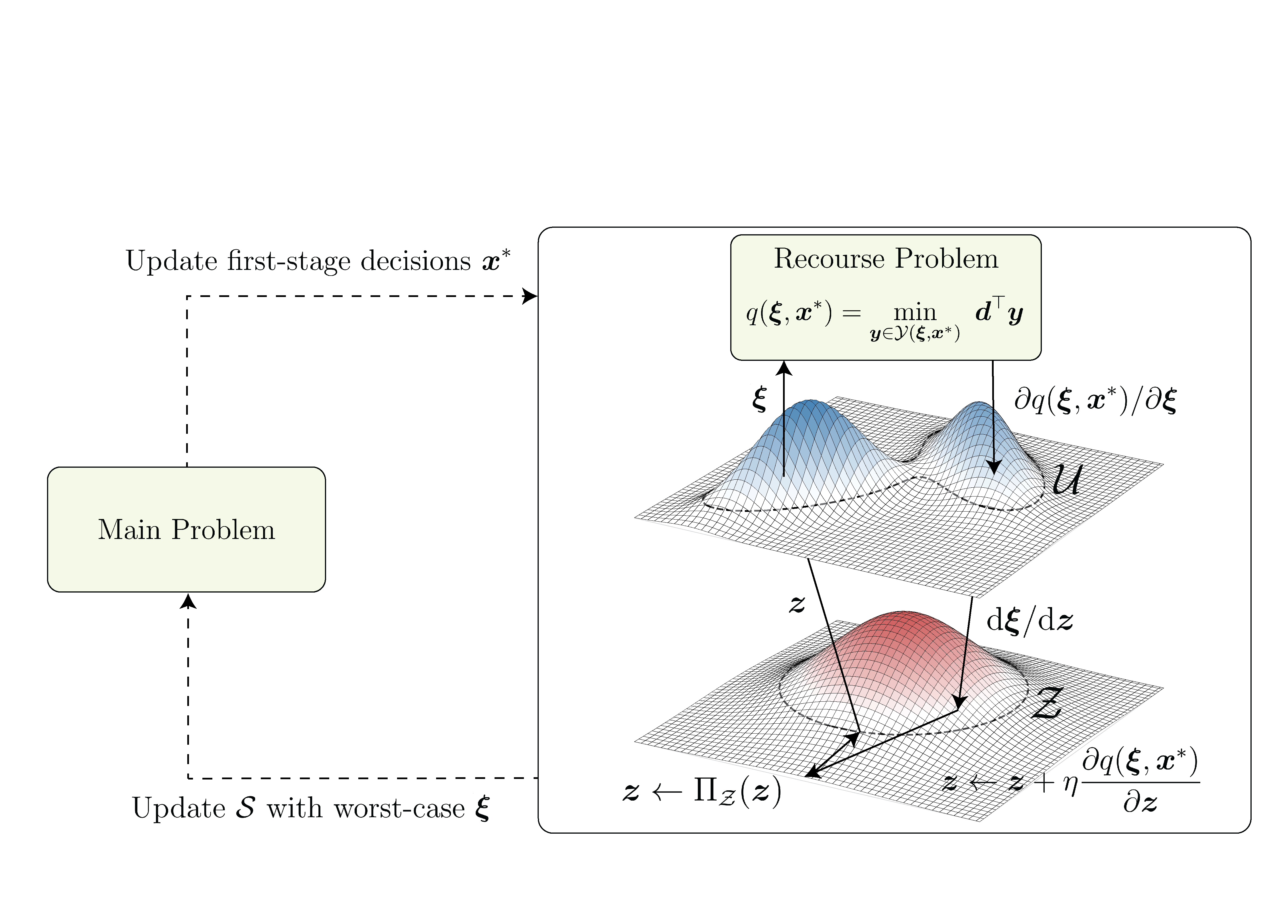
Figure 1: The AGRO solution algorithm. (i) First-stage decisions ${\bm{x}}^{*}$ are obtained by solving a main problem for a finite set of uncertainty realizations, $\mathcal{S}$. (ii) The latent variable ${\bm{z}}$ is sampled from within $\mathcal{Z}$ and decoded to obtain an initial ${\bm{\xi}}$. (iii) The recourse problem is solved given ${\bm{x}}^{*}$ and ${\bm{\xi}}$ and its optimal objective value is differentiated with respect to ${\bm{\xi}}$ and (after backpropagating through the decoder $f_{\theta}$) ${\bm{z}}$. (iv) A gradient ascent step is taken to update ${\bm{z}}$, which is then projected onto $\mathcal{Z}$ and decoded to obtain an updated ${\bm{\xi}}$. Steps (iii) and (iv) are iterated until converging to a worst-case ${\bm{\xi}}$. (v) The worst-case ${\bm{\xi}}$ is then added to $\mathcal{S}$, at which point the main problem is re-optimized.

3.1 Deep Data-Driven Uncertainty Sets

AGRO constructs tight uncertainty sets as nonlinear and differentiable transformations of spherical uncertainty sets lying in the latent space $\mathbb{R}^{L}$ with $L<D$, where $D$ is the dimensionality of ${\bm{\xi}}$. We approach learning these transformations as a VAE estimation task. Let ${\bm{z}}\sim\mathcal{N}({\bm{0}},{\bm{I}}_{L})$ be an isotropic Gaussian random variable and let $h_{\phi}:\mathbb{R}^{D}\to\mathbb{R}^{L}$ and $f_{\theta}:\mathbb{R}^{L}\to\mathbb{R}^{D}$ respectively denote the encoder and decoder of a VAE model trained to generate samples from $p_{\bm{\xi}}$ (Kingma and Welling, 2013). Specifically, $h_{\phi}$ is trained to map samples of uncertainty realizations to samples from $\mathcal{N}({\bm{0}},{\bm{I}}_{L})$ while $f_{\theta}$ is trained to perform the reverse mapping. Here, $L$ denotes the VAE bottleneck dimension, a hyperparameter that plays a large role in determining the fidelity and diversity of generated samples (see Appendix A.3) and is generally tuned through a process of trial and error. We note that our approach can be extended to other classes of deep generative models that learn such a mapping from $\mathcal{N}({\bm{0}},{\bm{I}}_{L})$ to $p_{\bm{\xi}}$ such as generative adversarial networks (Goodfellow et al., 2014), normalizing flows (Papamakarios et al., 2021), and diffusion models (Ho et al., 2020). However, we employ a VAE architecture as VAEs are known to exhibit relatively high stability in training and low computational effort for sampling (Bond-Taylor et al., 2021), making them highly conducive to integration within an optimization framework.

To construct the uncertainty set $\mathcal{U}$, we first consider a “latent” uncertainty set given by the $L$-ball $\mathcal{Z}\coloneqq\mathcal{B}({\bm{0}},\Gamma)$. We select the radius $\Gamma$ such that the decoded uncertainty set $\mathcal{U}=\{f_{\theta}({\bm{z}})\mid{\bm{z}}\in\mathcal{Z}\}$ satisfies $\mathbb{P}_{{\bm{\xi}}\sim p_{\bm{\xi}}}({\bm{\xi}}\in\mathcal{U})\geq\alpha$ with confidence level $\delta$. Letting ${\bm{\Xi}}\in\mathbb{R}^{N\times D}$ be our training dataset, we leverage Theorem 1 from Hong et al. (2021) to obtain $\Gamma$ according to the following steps.

1. Split ${\bm{\Xi}}$ into two disjoint sets: one with $N_{1}\geq\log\delta/\log\alpha$ samples reserved for calibrating the size of the uncertainty set (i.e., steps 2 and 3) and another with $(N-N_{1})$ samples for training the VAE.

2. After training the VAE, project the calibration data into the latent space and sort the resulting $L^{2}$ norms, i.e. $r_{j}\coloneqq\|h_{\phi}({\bm{\xi}}^{(j)})\|_{2}$ for all ${\bm{\xi}}^{(j)}$ in the calibration set, to obtain the order statistics of $\{r_{1},\dots,r_{N_{1}}\}$. We denote these order statistics by $r_{(1)}\leq\dots\leq r_{(N_{1})}$.

3. Choose $\Gamma=r_{(\ell)}$, where $j$ is defined as:

   $$\ell=\min_{1\leq j\leq N_{1}}\left\{j\ \Big{|}\ \sum_{k=0}^{i-1}{N_{1}\choose k}\alpha^{k}(1-\alpha)^{N_{1}-k}\geq 1-\delta\right\}.$$

This procedure effectively prescribes $\Gamma$ to be a robust (with respect to the sample size) $\alpha$-quantile estimate of the norm of encoded samples drawn from $p_{\bm{\xi}}$ with confidence level $\delta$. Fig. 2 shows a comparison of classical uncertainty sets against a tighter uncertainty set constructed by the proposed VAE-based method for samples from a nonunimodal bivariate distribution.

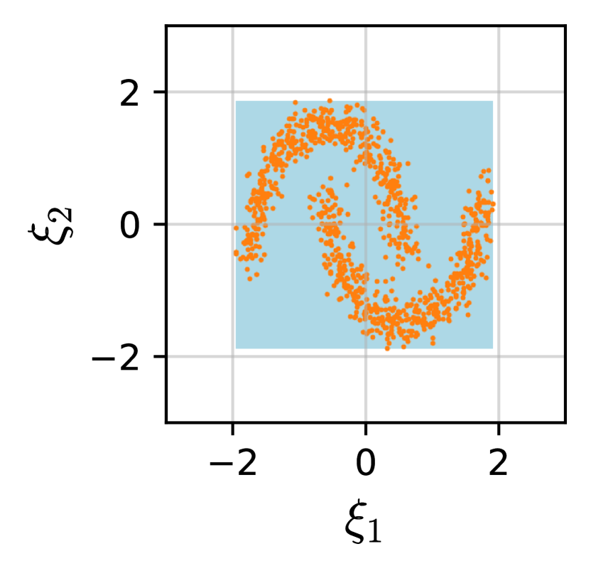
(a) Box

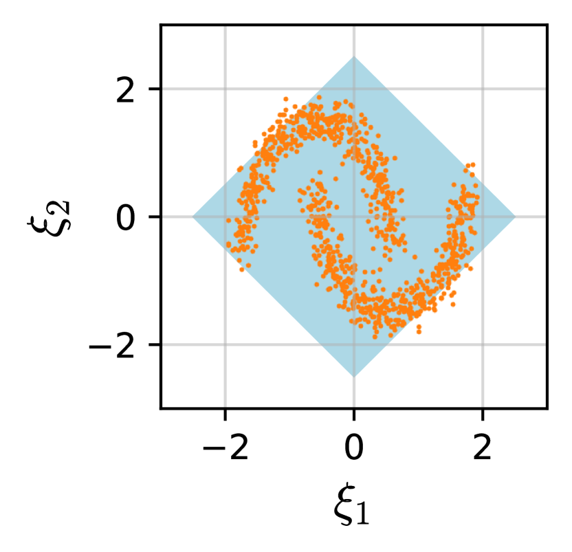
(b) Budget

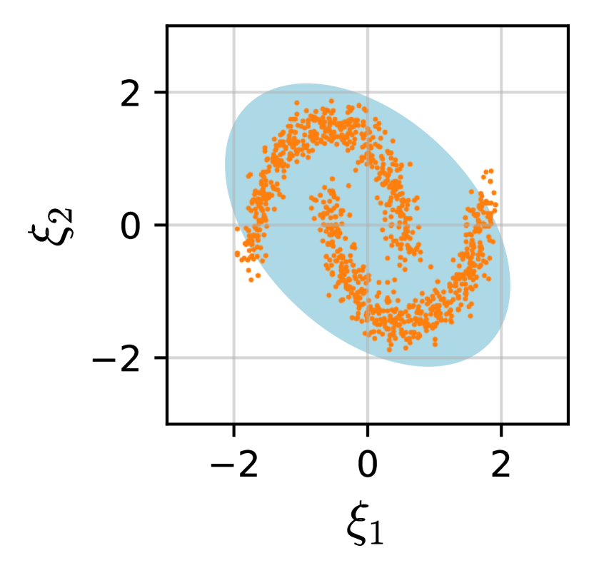
(c) Ellipsoidal

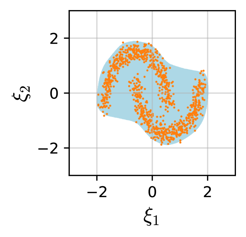
(d) VAE

Figure 2: A comparison of classical uncertainty sets (a)-(c) with the proposed VAE-learned uncertainty set (d) for an illustrative bivariate distribution. By covering a smaller region in $\mathbb{R}^{D}$, the VAE-learned uncertainty set (d) is more likely to yield a tighter approximation of the probabilistic constraint in equation 2 and less conservative first-stage decisions.

3.2 Adversarial Subproblem

Bilinear Formulation. As the main problem in AGRO is the same as Problem 3 for the classical CCG algorithm, we focus our discussion on the adversarial subproblem. Given a VAE decoder with ReLU activations $f_{\theta}:\mathbb{R}^{L}\to\mathbb{R}^{D}$, a latent uncertainty set $\mathcal{Z}=\mathcal{B}({\bm{0}},\Gamma)$, and the first-stage decisions ${\bm{x}}^{*}$, we formulate the adversarial subproblem as

$$\max_{{\bm{z}},\ {\bm{\xi}}}\ \left\{\ \min_{{\bm{y}}\in\mathcal{Y}({\bm{\xi}},{\bm{x}}^{*})}{\bm{d}}^{\top}{\bm{y}}\ \Big{|}\ {\bm{\xi}}=f_{\theta}({\bm{z}}),\ {\bm{z}}\in\mathcal{Z}\ \right\}.$$ (5)

To solve Problem 5, one can reformulate it as a single-level maximization problem by taking the dual of the recourse problem and maximizing the objective with respect to ${\bm{z}}$ subject to (1) optimality conditions (i.e., primal/dual feasibility and strong duality) of the recourse problem and (2) constraints encoding the input-output mapping for the ReLU decoder network, ${\bm{\xi}}=f_{\theta}({\bm{z}})$ (Fischetti and Jo, 2018). This formulation is presented in full as Problem 7 in Appendix A.2. As discussed in Sec. 2.2, however, this problem can be extremeley computationally demanding to solve. Therefore, we propose an alternative approach for solving Problem 5 based on PGA to efficiently obtain approximate solutions.

Projected Gradient Ascent Heuristic. Let $q:\mathbb{R}^{D}\times\mathcal{X}\to\mathbb{R}$ denote the optimal objective value of the recourse problem as a function of ${\bm{\xi}}$ and ${\bm{x}}$. It is then possible to differentiate $q$ with respect to ${\bm{\xi}}$ by implicitly differentiating the optimality conditions of the recourse problem at an optimal solution (Amos and Kolter, 2017). Doing so provides an ascent direction for maximizing $q$ with respect to ${\bm{z}}$ by backpropagating through $f_{\theta}$. As such, we maximize $q$ using PGA over $\mathcal{Z}$.

Specifically, to solve the adversarial subproblem using PGA, we first randomly sample an initial ${\bm{z}}$ from a distribution supported on $\mathcal{Z}$. We then transform ${\bm{z}}$ to obtain the uncertainty realization ${\bm{\xi}}=f_{\theta}({\bm{z}})$ and solve the recourse problem with respect to ${\bm{\xi}}$ to obtain $q({\bm{\xi}},{\bm{x}}^{*})$ and $\partial q({\bm{\xi}},{\bm{x}}^{*})/\partial{\bm{\xi}}$. Using automatic differentiation, we obtain the gradient of ${\bm{\xi}}$ with respect to ${\bm{z}}$ and perform the update:

$${\bm{z}}\leftarrow\Pi_{\mathcal{Z}}\left({\bm{z}}+\eta\frac{\partial q({\bm{\xi}},{\bm{x}}^{*})}{\partial{\bm{\xi}}}\frac{\differential{\bm{\xi}}}{\differential{\bm{z}}}\right),$$

where $\eta>0$ denotes the step-size hyperparameter and $\Pi_{\mathcal{Z}}$ denotes the projection operator given by $\Pi_{\mathcal{Z}}({\bm{z}})=\min\{\Gamma,\|{\bm{z}}\|_{2}\}\times{\bm{z}}/\|{\bm{z}}\|_{2}$. By projecting onto the set $\mathcal{Z}$ with radius $\Gamma$, we ensure that the solution to the adversarial subproblem is neither unrealistic nor overly adversarial. This procedure is repeated until convergence of $q(f_{\theta}({\bm{z}}),{\bm{x}}^{*})$ to a local maximum or another criterion (e.g., a maximum number of iterations) is met.

PGA is not guaranteed to converge to a worst-case uncertainty realization (i.e., global maximum of Problem 5) as $q(f_{\theta}({\bm{z}}),{\bm{x}}^{*})$ is nonconcave in ${\bm{z}}$. To escape local minima, we randomly initialize PGA with $I$ different samples of ${\bm{z}}$ in each iteration and select the worst-case uncertainty realization obtained after maximizing with PGA. We then update the set $\mathcal{S}$ and re-optimize the main problem to complete one iteration of AGRO. Additional iterations of AGRO are then performed until convergence of the main problem and adversarial subproblem objectives, i.e., $|\gamma-q(f_{\theta}({\bm{z}}),{\bm{x}}^{*})|<\epsilon$, for tolerance $\epsilon$. Algorithm 2 provides the full pseudocode for AGRO.

4 Experiments

To demonstrate AGRO’s efficacy in reducing planning costs, we apply our approach in two sets of experiments: a synthetic production-distribution problem and a real-world power system capacity expansion problem. For all experiments, we let $\alpha=0.95$ and fix the confidence level $\delta$ to be $0.05$ (see Sec. 3.1).

4.1 Production-Distribution Problem

Problem Description. We first apply AGRO to an adaptive robust production-distribution problem with synthetic demand data in order to evaluate its performance over a range of uncertainty distributions. We consider a two-stage problem in which the first-stage decisions ${\bm{x}}\in\mathbb{R}^{|\mathcal{I}|}$ correspond to the total number of items produced at each facility $i\in\mathcal{I}$ while second-stage decisions correspond to the quantities ${\bm{y}}\in\mathbb{R}^{|\mathcal{I}|\times|\mathcal{J}|}$ distributed to a set of demand nodes $\mathcal{J}$ after demands ${\bm{\xi}}\in\mathbb{R}^{|\mathcal{J}|}$ have been realized. Production incurs a unit cost of ${\bm{c}}$ in the first stage while shipping and unmet demand incur unit costs of ${\bm{d}}\in\mathbb{R}^{|\mathcal{I}|\times|\mathcal{J}|}$ and $d^{\prime}\in\mathbb{R}$ respectively. Here, transportation costs vary by origin and destination while the cost of unmet demand is uniform across nodes.

Experimental Setup. In each experiment, we generate the demand dataset ${\bm{\Xi}}\in\mathbb{R}^{N\times|\mathcal{J}|}$ by drawing samples from a Gaussian mixture distribution with $3$ correlated components. We vary the problem size over the range $(|\mathcal{I}|,|\mathcal{J}|)\in\{(4,3),(8,6),(12,9),(16,12)\}$, and perform $50$ experimental trials for each problem size. In each trial, we sample a dataset of $2500$ samples, each of which is then divided into a $1000$-sample VAE training set (split $80/20$ for model training/validation), $500$-sample $\Gamma$-calibration set, and $1000$-sample test set. Additional implementation details are provided in Appendix B.1.

Towards understanding how the VAE bottleneck dimension informs optimization outcomes, we vary $L\in\{1,2,4\}$. We report standard generative fidelity and diversity metrics for trained VAEs in Appendix B.1.1. To evaluate costs, we fix the solved investment decision ${\bm{x}}$ and compute ${\bm{c}}^{\top}{\bm{x}}+\hat{F}^{-1}(\alpha;{\bm{x}})$, where $\hat{F}^{-1}(\alpha;{\bm{x}})$ is the $\alpha$-quantile of recourse costs obtained over the test set given ${\bm{x}}$. We compare cost and runtime results obtained by AGRO to those obtained by a classical CCG algorithm, for which we consider both budget and ellipsoidal uncertainty sets with sizes calibrated according to the approach described by Hong et al. (2021).

Results. The relative improvement in out-of-sample costs (i.e., ${\bm{c}}^{\top}{\bm{x}}+\hat{F}^{-1}(\alpha;{\bm{x}})$) obtained by AGRO in comparison to CCG is shown in Figure 3. Cost comparisons for CCG with ellipsoidal uncertainty sets are omitted for the cases with $|\mathcal{J}|>6$ as the resulting CCG subproblem could not be solved to optimality within the time limit of $900$ seconds. Figure 3 shows that AGRO’s relative advantage over classical CCG in minimizing costs grows as the dimensionality of uncertainty increases. This is expected as classical uncertainty sets are known to provide looser approximations of probabilistic constraints in higher dimensional settings (Lam and Qian, 2019). Runtime results provided in Table 2 (see Appendix B.1.1) also show that runtimes for AGRO scale much better than those for CCG with a budget uncertainty set. In particular, CCG is solved $80$ times faster than AGRO with $L=4$ for $|\mathcal{J}|=3$ but is about $10$ times slower than AGRO with $L=4$ for $|\mathcal{J}|=12$.

The effect of the VAE bottleneck dimension on out-of-sample costs can be observed from the box-plot in Figure 3. In particular, solutions obtained from AGRO using VAEs with $L=4$ outperform classical CCG more consistently than solutions obtained with $L<4$. This is likely due to the fact that VAEs with $L=4$ achieve a greater coverage of $p_{\bm{\xi}}$ (see Table 4 in Appendix B.1.1), and consequently, will consistently yield uncertainty sets that satisfy the probabilistic constraint. On the other hand, models with lower bottleneck dimensions are more prone to “overlooking” adversarial realizations due to inadequate coverage of $p_{\bm{\xi}}$, which causes occasional underestimation of worst-case recourse costs and under-production in the first stage. However, this effect is reversed in the low-dimensional case of $|\mathcal{J}|=3$ as VAEs with higher bottleneck dimensions, which score lower on generative fidelity metrics (see Table 3), over-produce in the first stage in anticipation of highly adversarial yet unrealistic demand realizations.

		$|\mathcal{J}|$
$L$	CCG  $\mathcal{U}$	3	6	9	12
$1$	Budg.	0.77%	0.98%	1.14%	1.51%
	Ellips.	0.41%	0.51%	—	—
$2$	Budg.	0.75%	1.17%	1.50%	1.74%
	Ellips.	0.39%	0.71%	—	—
$4$	Budg.	0.55%	1.08%	1.56%	1.77%
	Ellips.	0.19%	0.61%	—	—

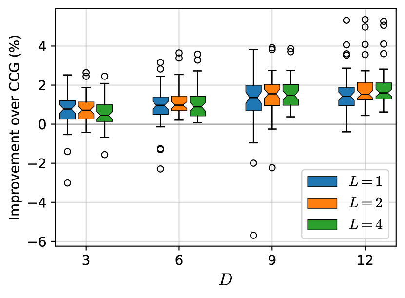
Figure 3: (Left): Average cost improvement for AGRO over CCG with budget and ellipsoidal uncertainty sets. (Right): Box-plots showing relative improvement for AGRO over CCG with budget uncertainty. The relative cost advantage of VAE-learned uncertainty sets over classical uncertainty sets increases with the dimensionality of uncertainty.

4.2 Capacity Expansion Planning

We now consider the problem of robust capacity expansion planning for a regional power system with historical renewable capacity factor and energy demand data. Capacity expansion models are a centerpiece for long-term planning of energy infrastructure under supply, demand, and cost uncertainties (Zhang et al., 2024; Roald et al., 2023). A number of works have adopted ARO formulations for energy systems planning with a particular focus on ensuring system reliability under mass adoption of renewable energy with intermittent and uncertain supply (Ruiz and Conejo, 2015; Amjady et al., 2017; Minguez et al., 2017; Abdin et al., 2022). In models with high spatiotemporal resolutions, supply and demand uncertainties are complex, high-dimensional, and nonunimodal, exhibiting nonlinear correlations such as temporal autocorrelations and spatial dependencies. These patterns cannot be accurately captured by classical uncertainty sets. As a result, tightening uncertainty representations for robust capacity expansion planning has the potential to significantly lower investment costs over conventional ARO methods while still maintaining low operational costs day-to-day.

Problem Description. We use AGRO to solve a two-stage adaptive robust generation and transmission expansion planning problem for the New England transmission system. The model we consider most closely follows that of (Minguez et al., 2017) and has two stages: an initial investment stage and a subsequent economic dispatch (i.e., recourse) stage. The objective function is a weighted sum of investment costs plus annualized worst-case economic dispatch costs. We let $\mathcal{N}$, $\mathcal{T}$, and $\mathcal{P}$ denote the set of nodes, hourly operational periods, and renewable energy sources respectively; here, $|\mathcal{N}|=6$, $|\mathcal{T}|=24$, and $|\mathcal{P}|=3$. Investment decisions for this problem include installed capacities for (1) dispatchable, solar, onshore wind, and offshore wind power plants for all nodes, (2) battery storage at each node, and (3) transmission capacity for all edges in $\mathcal{N}\times\mathcal{N}$. The economic dispatch stage occurs after the realization of demand and renewable capacity factors, ${\bm{\xi}}\in\mathbb{R}^{|\mathcal{N}||\mathcal{T}||\mathcal{P}|}$. This stage determines optimal hourly generation, power flow, and storage decisions to minimize the combined cost of load shedding and variable costs for dispatchable generation; these decisions are subject to ramping, storage, and flow balance constraints. The full formulations for both stages are presented in Appendix B.2.

Experimental Setup. After processing features (see Appendix B.2), we have a dataset with $N=7300$ samples and $D=349$ distinct features. Results are obtained over a five-fold cross-validation with each fold having $6200$ VAE training samples (split 80/20 for model training/validation), $100$ $\Gamma$-calibration samples, and $1000$ test samples. Similarly to Sec. 4.1, we evaluate costs by fixing solved investment decisions and computing the $\alpha$-quantile of economic dispatch costs over the test set. We consider a ball-box latent uncertainty set for AGRO, which intersects the latent uncertainty set described in Sec. 3.1 with a box uncertainty set in the latent space (i.e., $\min_{i}h_{\phi}({\bm{\Xi}}_{i,:})_{j}\leq z_{j}\leq\max_{i}h_{\phi}({\bm{\Xi}}_{i,:})_{j}$ for $j=1,\dots,L$). We compare AGRO against a classical CCG algorithm using a budget-box uncertainty set, which is commonly used in the power systems literature (Bertsimas et al., 2012; Ruiz and Conejo, 2015; Amjady et al., 2017; Abdin et al., 2022). However, we do not report results obtained using an ellipsoidal uncertainty set as the corresponding CCG subproblem could not be solved to optimality within the time limit of $900$ seconds. As was the case in Sec. 4.1, we report results for a range of VAE bottleneck dimensions: $L\in\{2,4,8,16\}$.

	VaR Obj	ARO Obj	Error	Total	Train	SP
CCG	10.624	13.597	55.1%	5326	—	22
$L=2$	9.392	9.287	14.8%	650	191	55
$L=4$	9.735	11.123	28.2%	2578	219	282
$L=8$	9.757	10.505	33.2%	2860	251	426
$L=16$	10.063	12.229	49.1%	2016	208	382

Table 1: AGRO and CCG cost and runtime performance estimates averaged over all folds. VaR Obj denotes the sample-estimated $\mathrm{VaR}$ objective value, ${\bm{c}}^{\top}{\bm{x}}^{*}+\hat{F}^{-1}(\alpha;{\bm{x}})$, while ARO Obj denotes the objective value of the main problem, ${\bm{c}}^{\top}{\bm{x}}^{*}+\gamma^{*}$ (both in units of $ billions). Error denotes the mean absolute percent error of worst-case recourse costs obtained by the subproblem compared to an out-of-sample $\mathrm{VaR}$ estimate of recourse costs averaged over all iterations and folds. Total, Train, and SP respectively denote average total runtime (including training), average training runtime, and average subproblem runtime in seconds.

Results. Table 1 reports cost, runtime, and $\mathrm{VaR}$ approximation error results for our AGRO and CCG implementations. For all tested bottleneck dimensions, AGRO obtains investment decisions that yield lower total costs compared to CCG as evaluated over the test set. In particular, costs are minimized by AGRO with $L=2$, which yields an 11.6% average reduction in total costs over CCG. For all $L$, the average total runtime for AGRO, which includes VAE training time, is also observed to be less than that of CCG.

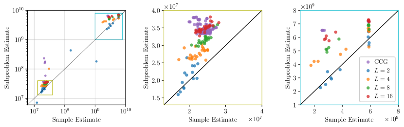
Figure 5: Comparison of sample-estimated VaR, $\hat{F}^{-1}(\alpha;{\bm{x}}^{*})$, and estimated worst-case costs obtained from solving the adversarial subproblem, $f({\bm{\xi}}^{i},{\bm{x}}^{*})$. Each point is obtained from one iteration of AGRO/CCG. Points that are closer to the diagonal line indicate a more accurate estimate of VaR. The middle and right-hand plots provide a zoomed-in view of two regions with a high concentration of points. Subproblem estimates are always greater than sample estimates except in the case of AGRO with $L=2$ (blue).

To empirically evaluate the tightness of VAE-learned and classical uncertainty sets with respect to approximating value-at-risk, we compare the relative error of worst-case recourse costs obtained by the adversarial subproblems (i.e., $q({\bm{\xi}}^{i},{\bm{x}}^{*})$) with out-of-sample $\mathrm{VaR}$ estimates (i.e., $\hat{F}^{-1}(\alpha;{\bm{x}}^{*})$) for all iterations. Table 1 shows that worst-case recourse costs obtained by AGRO with $L=2$ most closely approximate the true value-at-risk. We visualize this phenomenon by plotting worst-case recourse costs against $\mathrm{VaR}$ estimates obtained in all iterations in Fig. 5 (see Appendix B.2.1). Fig. 5 shows that AGRO consistently overestimates $\mathrm{VaR}$ when $L\geq 4$, which provides empirical support that the VAE-learned uncertainty sets provide a safe approximation for the probabilistic constraint in equation 2. The VAEs trained with $L=2$ – despite yielding the lowest average costs – achieve a much lower coverage of $p_{\bm{\xi}}$ than other models (see Fig. 5 in Appendix B.2.1). This effectively reduces the effective size of $\mathcal{U}$ to contain less than $\alpha$ probability mass of $p_{\bm{\xi}}$ and prevents $\mathcal{U}$ from serving as a safe approximation for the probabilistic constraint.

Taken together, these results suggests that while poor generative diversity can cause AGRO to “overlook” cost-maximizing realizations – which we observed as contributing to costly under-production for the production-distribution case study – the end result is not necessarily a catastrophic under-estimation of costs. The quality of solved first-stage decisions depends highly on the quality of the underlying VAE as a generative model. However, the ideal choice of $L$ is not necessarily one that optimizes standard evaluation metrics for generative modeling, and consequently, should be tuned with respect to both downstream optimization outcomes.

Finally, we visualize AGRO’s advantage over CCG in avoiding unrealistic cost-maximizing contingencies by plotting solved worst-case realizations for CCG and AGRO in Fig. 4. Here, CCG generates an uncertainty realization in which solar and wind capacity factors drop sharply to zero before immediately rising to their nominal values. Additionally, weather-related correlations between variables are not maintained; most notably, the positive correlation between load and solar capacity factors as well as the spatial correlation of load across the system are not observed. Accounting for these supply and demand features during investment planning is essential for effectively leveraging the complementarities between generation, storage, and transmission. On the other hand, AGRO is able to identify uncertainty realizations that are simultaneously cost-maximizing and realistic. This can be observed from the way in which selected realizations demonstrate realistic temporal autocorrelation (i.e., smoothness) and show a less improbable combination of low capacity factors with moderate load.

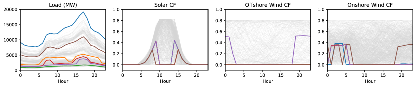
(a) CCG Uncertainty Realization

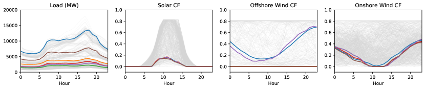
(b) AGRO ($L=4$) Uncertainty Realization

Figure 4: Comparison of worst-case uncertainty realizations as obtained by (a) CCG and (b) AGRO with $L=4$. Different colors are used to represent each of the six nodes in the power system. Realizations corresponding to a random sample of 100 observations are shown in gray.

5 Conclusion

Increasing availability of data for operations of large-scale systems has inspired growing interest in data-driven optimization for planning. This paper proposes AGRO, a novel data-driven method for two-stage ARO that integrates a VAE within an optimization framework to generate realistic and adversarial realizations of operational uncertainties. Our method builds on the classical CCG algorithm for two-stage ARO problems by leveraging differentiable optimization methods to identify cost-maximizing uncertainty realizations over a VAE-learned uncertainty set. We demonstrate empirically that AGRO is effective in tightly approximating a value-at-risk constraint for recourse costs, and consequently, is able to reduce total costs by up to 1.8% in a synthetic production-distribution problem and up to 11.6% in a regional power system expansion problem using historical energy supply/demand data.

Appendix A Methodological Details

A.1 Uncertainty Sets

The box, budget, and ellipsoidal uncertainty sets are constructed in a data-driven setting as

$$\mathcal{U}^{\text{box}} =\Big{\{}{\bm{\xi}}\in\mathbb{R}^{D}\ \mid\ \hat{{\bm{\xi}}}^{\text{min}}\leq{\bm{\xi}}\leq\hat{{\bm{\xi}}}^{\text{max}}\Big{\}}$$ (6a)

$$\mathcal{U}^{\text{budget}} =\Big{\{}{\bm{\xi}}\in\mathbb{R}^{D}\ \mid\ \sum_{i=1}^{D}\hat{\Sigma}_{ii}^{-1}|{\bm{\xi}}_{i}-\hat{\mu}_{i}|\leq\Gamma_{\text{budget}}\Big{\}}$$ (6b)

$$\mathcal{U}^{\text{ellipse}} =\Big{\{}{\bm{\xi}}\in\mathbb{R}^{D}\ \mid\ ({\bm{\xi}}-\hat{{\bm{\mu}}})^{\top}\hat{{\bm{\Sigma}}}^{-1}({\bm{\xi}}-\hat{{\bm{\mu}}})\leq\Gamma_{\text{ellipse}}\Big{\}}.$$ (6c)

Here, $\hat{{\bm{\mu}}}$, $\hat{{\bm{\Sigma}}}$, $\hat{{\bm{\xi}}}^{\text{min}}$, and $\hat{{\bm{\xi}}}^{\text{max}}$ denote the empirical mean, covariance, minimum value, and maximum value of ${\bm{\xi}}$ observed from the dataset while the $\Gamma$ parameters denote the uncertainty “budgets.”

A.2 Bilevel Formulation for AGRO

Letting ${\bm{\pi}}$ denote the dual variables of the recourse problem, the max-min problem 5 can be reformulated as the following mixed-binary bilinear program:

$$\max\quad {\bm{d}}({\bm{\xi}})^{\top}{\bm{y}}$$ (7a)

$$\mathrm{s.t.}\quad {\bm{B}}({\bm{\xi}}){\bm{y}}\geq{\bm{b}}({\bm{\xi}})-{\bm{A}}({\bm{\xi}}){\bm{x}}^{*},$$ (7b)

$${\bm{\pi}}^{\top}{\bm{B}}({\bm{\xi}})\leq{\bm{d}}({\bm{\xi}}),$$ (7c)

$${\bm{y}},{\bm{\pi}}\geq{\bm{0}},$$ (7d)

$${\bm{\pi}}^{\top}({\bm{b}}({\bm{\xi}})-{\bm{A}}({\bm{\xi}}){\bm{x}}^{*})={\bm{d}}({\bm{\xi}})^{\top}{\bm{y}},$$ (7e)

$$\|{\bm{z}}\|_{2}\leq\Gamma,$$ (7f)

$${\bm{W}}^{(0)}{\bm{z}}+{\bm{b}}^{(0)}={\bm{z}}^{(1)}-\tilde{{\bm{z}}}^{(1)},$$ (7g)

$${\bm{W}}^{(\ell)}{\bm{z}}^{(\ell)}+{\bm{b}}^{(\ell)}={\bm{z}}^{(\ell+1)}-\tilde{{\bm{z}}}^{(\ell+1)}, \ell\in[K-1]$$ (7h)

$${\bm{W}}^{(K)}{\bm{z}}^{(K)}+{\bm{b}}^{(K)}={\bm{\xi}},$$ (7i)

$$a_{j}^{(\ell)}=1\implies z_{j}^{(\ell)}=0, j\in[D_{\ell}],\ \ell\in[K-1]$$ (7j)

$$a_{j}^{(\ell)}=0\implies\tilde{z}_{j}^{(\ell)}=0, j\in[D_{\ell}],\ \ell\in[K-1]$$ (7k)

$${\bm{z}}^{(\ell)},\tilde{{\bm{z}}}^{(\ell)}\geq{\bm{0}}, \ell\in[K]$$ (7l)

$${\bm{a}}^{(\ell)}\in\{0,1\}^{D_{\ell}}. \ell\in[K-1]$$ (7m)

Here, constraints 7b and 7c respectively enforce primal and dual feasibility, constraint 7d enforces nonnegativity of the primal and dual variables, and constraint 7e enforces strong duality. Together, constraints 7b–7e provide sufficient conditions for optimality of the recourse problem. Constraint 7f enforces ${\bm{z}}\in\mathcal{Z}$ to bound the range of uncertainty realizations that are considered. Additionally, we apply the main result of Fischetti and Jo [2018] to embed the mapping ${\bm{\xi}}=f_{\theta}({\bm{z}})$ by introducing the binary decision variables $\{{\bm{a}}^{(\ell)}\}_{\ell\in[K-1]}$ and real-valued decision variables $\{{\bm{z}}^{(\ell)},\tilde{{\bm{z}}}^{(\ell)}\}_{\ell\in[K]}$ through constraints 7g–7m. Here, $D_{\ell}$ denotes the number of output units in layer $\ell$ while ${\bm{W}}^{(\ell)}\in\mathbb{R}^{D_{\ell+1}\times D_{\ell}}$ and ${\bm{b}}^{(\ell)}\in\mathbb{R}^{D_{\ell+1}}$ denote the weight matrix and offset parameters of layer $\ell$. Note that, for any ${\bm{x}}\in\mathcal{X}$, Problem 7 is feasible as a consequence of the primal feasibility (i.e., complete recourse) and boundedness assumptions.

A.3 Fidelity and Diversity Metrics

We quantify performance of the VAEs as generative models for $p_{\bm{\xi}}$ using standard metrics for fidelity (precision and density) and diversity (recall and coverage). Semantically, fidelity can be understood as measuring the “realism” of generated samples while diversity can be understood as measuring the breadth of generated samples. These metrics are formally defined by Naeem et al. [2020] as follows:

precision $$=\frac{1}{M}\sum_{j=1}^{M}\mathbbm{1}_{\hat{{\bm{\xi}}}^{(j)}\in\text{manifold}({\bm{\xi}}^{(1)},\dots,{\bm{\xi}}^{(N)})}$$

density $$=\frac{1}{kM}\sum_{j=1}^{M}\sum_{i=1}^{N}\mathbbm{1}_{\hat{{\bm{\xi}}}_{j}\in\mathcal{B}({\bm{\xi}}^{(i)},\mathrm{NND}_{k}({\bm{\xi}}^{(i)}))}$$

recall $$=\frac{1}{N}\sum_{i=1}^{N}\mathbbm{1}_{{\bm{\xi}}_{i}\in\text{manifold}(\hat{{\bm{\xi}}}^{(1)},\dots,\hat{{\bm{\xi}}}^{(M)})}$$

coverage $$=\frac{1}{N}\sum_{i=1}^{N}\mathbbm{1}_{\exists\ j\ \text{s.t.}\ \hat{{\bm{\xi}}}^{(j)}\in\mathcal{B}({\bm{\xi}}^{(i)},\mathrm{NND}_{k}({\bm{\xi}}^{(i)}))},$$

where ${\bm{\xi}}$ and $\hat{{\bm{\xi}}}$ respectively denote real ($N$ total) and generated samples ($M$ total), $\mathbbm{1}$ denotes the indicator function, $\mathrm{NND}_{k}({\bm{\xi}}^{(i)})$ denotes the distance from ${\bm{\xi}}^{(i)}$ to its $k$-th nearest neighbor (excluding itself) in the dataset $\{{\bm{\xi}}^{(1)},\dots,{\bm{\xi}}^{(N)}\}$, and manifolds are defined as

$$\text{manifold}({\bm{\xi}}^{(1)},\dots,{\bm{\xi}}^{(N)})=\bigcup_{i=1}^{N}\mathcal{B}({\bm{\xi}}^{(i)},\mathrm{NND}_{k}({\bm{\xi}}^{(i)})).$$

Precision and density quantify the portion of generated samples that are “covered” by the real samples while recall and coverage quantify the portion of real samples that are “covered” by the generated samples. All results for both sets of experiments are obtained over the held-out test datasets using $k=5$ and with $M=N=1000$.

A.4 AGRO Algorithm

Algorithm 1 AGRO

1:Decoder $f_{\theta}$, Uncertainty Set $\mathcal{Z}$, Step-size $\eta$, Initializations $I$, Convergence tolerance $\epsilon$

2:Optimal solution ${\bm{x}}^{*}$

3:Initialize Scenario set $\mathcal{S}\leftarrow\emptyset$, Iteration counter $i\leftarrow 1$

4:while not converged do

5:    ${\bm{x}}^{*},\gamma\leftarrow\operatorname*{arg\,min}_{{\bm{x}}\in\mathcal{X},\gamma}\{{\bm{c}}^{\top}{\bm{x}}+\gamma\mid q({\bm{\xi}}^{i},{\bm{x}})\leq\gamma,\ \forall{\bm{\xi}}^{i}\in\mathcal{S}\}$ $\triangleright$ Solve main problem

6:    for $j=1$ to $I$ do $\triangleright$ Solve adversarial subproblem

7:         Sample ${\bm{z}}^{j}$ from $\mathcal{Z}$

8:         while not converged do

9:             Decode ${\bm{\xi}}=f_{\theta}({\bm{z}}^{j})$

10:             Solve recourse problem for $q({\bm{\xi}},{\bm{x}}^{*})$

11:             ${\bm{z}}^{j}\leftarrow\Pi_{\mathcal{Z}}\left({\bm{z}}^{j}+\eta\frac{\partial q({\bm{\xi}},{\bm{x}}^{*})}{\partial{\bm{\xi}}}\frac{\differential{\bm{\xi}}}{\differential{\bm{z}}^{j}}\right)$

12:         end while

13:    end for

14:    $j^{*}\leftarrow\operatorname*{arg\,max}_{j\in\{1,\dots,I\}}q(f_{\theta}({\bm{z}}^{j}),{\bm{x}}^{*})$ $\triangleright$ Select worst-case realization

15:    Set ${\bm{\xi}}^{i}\leftarrow f_{\theta}({\bm{z}}^{j^{*}})$

16:    if $q({\bm{\xi}}^{i},{\bm{x}}^{*})\leq\gamma$ then $\triangleright$ Check convergence

17:         Terminate and return ${\bm{x}}^{*}$

18:    else

19:         Update $\mathcal{S}\leftarrow\mathcal{S}\cup\{{\bm{\xi}}^{i}\}$ $\triangleright$ Add worst-case realization to scenario set

20:         Increment $i\leftarrow i+1$

21:    end if

22:end while

23:return $x^{*}$

Algorithm 2 AGRO Algorithm

Appendix B Experimental Details

B.1 Production-Distribution Problem

Formulation. We formulate the two-stage production-distribution problem as

$$\min_{{\bm{x}}}\quad \sum_{i\in\mathcal{I}}c_{i}x_{i}+\max_{{\bm{\xi}}\in\mathcal{U}}q({\bm{\xi}},{\bm{x}})$$ (8a)

$$\mathrm{s.t.}\quad {\bm{x}}\geq{\bm{0}},$$ (8b)

where the recourse cost $q({\bm{\xi}},{\bm{x}})$ is given as the solution to the following linear program:

$$q({\bm{\xi}},{\bm{x}})=\min_{\bm{y}}\quad \sum_{i\in\mathcal{I}}\sum_{j\in\mathcal{J}}d_{ij}^{1}y_{ij}^{1}+\sum_{j\in\mathcal{J}}d^{2}y_{j}^{2}$$ (9a)

$$\mathrm{s.t.}\quad \sum_{i\in\mathcal{I}}y_{ij}^{1}+y_{j}^{2}\geq\xi_{j}, j\in\mathcal{J}$$ (9b)

$$\sum_{j\in\mathcal{J}}y_{ij}\leq p_{i}x_{i}, i\in\mathcal{I}$$ (9c)

$${\bm{y}}^{1},{\bm{y}}^{2}\geq{\bm{0}}.$$ (9d)

This problem is adapted as a continuous relaxation (with respect to the first-stage decisions) of the facility location problem introduced by Bertsimas and Kim [2024]. Here, the first-stage decisions are the real-valued decision variables $x_{i}$ determining the amount of items to produce at facility $i$ at a unit cost of $c_{i}$ for all $i\in\mathcal{I}$. After the demands $\xi_{j}$ for all delivery destinations $j\in\mathcal{J}$ are realized, items are shipped from facilities to delivery destinations at a unit cost of $d_{ij}$ for facility $i$ and destination $j$. These shipment quantities are captured for $i\in\mathcal{I}$ and $j\in\mathcal{J}$ by the continuous recourse decision variables $y_{ij}$. An additional penalty is incurred for any unmet demand $y_{j}^{2}$ at destination $j$ with unit cost $d^{2}$. Constraints 9b define $y_{j}^{2}$ as unmet demand while constraints 9c ensure the total number of items shipped from a facility $i$ does not exceed its production, $p_{i}x^{i}$, where $p_{i}$ is the production factor for facility $i$.

Generating Instances. In each trial, we randomly sample both mean and covariance parameters of the Gaussian mixture $p_{\bm{\xi}}$ as well as parameters of the production-distribution problem, ${\bm{c}}$, ${\bm{d}}$ and, ${\bm{p}}$ ($d^{\prime}$ is fixed to $5$ in all iterations). To define the Gaussian mixture distribution $p_{\bm{\xi}}$, we first sample the mixing parameters ${\bm{\zeta}}\in[0,1]^{3}$ from a symmetric Dirichlet distribution, i.e., ${\bm{\zeta}}\sim\mathrm{Dir}({\bm{1}})$. For each component $k=1,\dots,3$, we sample the population mean ${\bm{\mu}}^{k}\sim\mathcal{N}({\bm{0}},|\mathcal{J}|{\bm{I}}_{|\mathcal{J}|})$ and the population covariance ${\bm{\Sigma}}^{k}$ from the Wishart distribution with $|\mathcal{J}|$ degrees of freedom and identity scale matrix ${\bm{I}}_{|\mathcal{J}|}$. To generate the problem parameters ${\bm{c}}\in\mathbb{R}^{|\mathcal{I}|}$, ${\bm{d}}\in\mathbb{R}^{|\mathcal{I}|\times|\mathcal{J}|}$ and, ${\bm{p}}\in\mathbb{R}^{|\mathcal{I}|}$, we follow the procedure described by Bertsimas and Kim [2024]. Specifically, we sample ${\bm{d}}$ uniformly at random from the interior of the ball $\mathcal{B}(\overline{{\bm{d}}},1.5)$ where $\overline{d}_{i}\sim\mathrm{Unif}(2,22)$ for $i\in\mathcal{I}$. We then sample $p_{i}\sim\mathrm{Unif}(8,18)$ and $c_{i}\sim\mathrm{Unif}(2,4)$ for $i\in\mathcal{I}$.

Computational Details. Both the encoder and decoder of our VAE correspond to three-layer networks with $\mathrm{ReLU}$ activations and are trained on the MIT Supercloud system [Reuther et al., 2018] using an Intel Xeon Gold 6248 machine with 40 CPUs and two 32GB NVIDIA Volta V100 GPUs, which takes approximately 30 seconds for all instances. All optimization is also performed on the MIT Supercloud system [Reuther et al., 2018] using an Intel Xeon Platinum 8260 machine with 96 cores and using Gurobi 11 [Gurobi Optimization, LLC, 2023] except when solving the AGRO subproblem, in which case results are obtained using the Cvxpylayers package [Agrawal et al., 2019].

To solve the adversarial subproblem with AGRO, we perform $10$ random initializations of ${\bm{z}}$. For each initialization, we perform normalized PGA with a learning rate of $\eta=0.1$ until either (a) costs obtained in successive PGA steps have converged within a tolerance of $0.01\%$ or (b) $1000$ PGA steps have been performed. If the worst-case realization ${\bm{\xi}}$ obtained over all $10$ initializations does not exceed the lower bound obtained by the most recent iteration of the master problem (i.e., $\gamma$), we perform additional initializations until either (a) a new worst-case realization is obtained or (b) $200$ initializations have been performed (in which case, AGRO terminates).

B.1.1 Experimental Results

$|\mathcal{I}|$	$|\mathcal{J}|$	Budget	Ellipsoid	AGRO ($L=1$)	AGRO ($L=2$)	AGRO ($L=4$)
4	3	1.13	1.13	11.93	46.61	84.77
8	6	7.1	371.18	13.8	45.53	109.69
12	9	250.09	—	16.29	73.85	115.08
16	12	1199.22	—	26.91	76.59	113.4

Table 2: Runtime results for production-distribution problem (not including VAE training).

	$|J|=3$		$|J|=6$		$|J|=9$		$|J|=12$
$L$	Precision	Recall	Precision	Recall	Precision	Recall	Precision	Recall
1	0.98	1.08	0.98	1.43	0.97	1.94	0.97	2.65
2	0.98	1.05	0.95	1.22	0.93	1.56	0.93	2.1
4	0.97	1.0	0.94	1.09	0.92	1.36	0.92	1.78

Table 3: Fidelity metrics for VAEs trained using the production-distribution problem data averaged over all $50$ instances.

	$|J|=3$		$|J|=6$		$|J|=9$		$|J|=12$
$L$	Density	Coverage	Density	Coverage	Density	Coverage	Density	Coverage
1	0.08	0.32	0.01	0.28	0.01	0.3	0.0	0.34
2	0.78	0.83	0.32	0.66	0.15	0.65	0.08	0.67
4	0.96	0.95	0.89	0.93	0.61	0.89	0.37	0.88

Table 4: Diversity metrics for VAEs trained using the production-distribution problem data averaged over all $50$ instances.

B.2 Capacity Expansion Model

The capacity expansion model is given by

$$\min_{{\bm{x}}}\quad \sum_{i\in\mathcal{N}}c^{d}x_{i}^{d}+\sum_{i\in\mathcal{N}}\sum_{p\in\mathcal{P}}c^{p}x_{i}^{p}+\sum_{i\in\mathcal{N}}c^{b}x_{i}^{b}+\sum_{(i,j)\in\mathcal{E}}c^{\ell}x_{ij}^{\ell}+\lambda\max_{{\bm{\xi}}\in\mathcal{U}}q({\bm{\xi}},{\bm{x}})$$ (10a)

s.t. $$\sum_{i\in\mathcal{N}}x_{i}^{p}\leq\Gamma^{p} p\in\mathcal{P}$$ (10b)

$$x_{i}^{d}\leq\Gamma^{d} i\in\mathcal{N}$$ (10c)

$$x_{ij}^{\ell}\leq\Gamma_{ij}^{\ell} (i,j)\in\mathcal{E}$$ (10d)

$${\bm{x}}^{d}\in\mathbb{Z}_{\geq 0}^{|\mathcal{N}|}$$ (10e)

$${\bm{x}}^{d},{\bm{x}}^{b},{\bm{x}}^{\ell}\geq{\bm{0}}.$$ (10f)

Here the first-stage node-level decision variables include installed dispatchable generation capacity ($x_{i}^{d}\in\mathbb{Z}_{+}$), installed renewable plant capacity ($x_{i}^{p}\geq 0$) for renewable technologies $p\in\mathcal{P}$, and installed battery storage capacity $(x_{i}^{b}\geq 0)$. Additionally, we consider transmission capacity ($x_{ij}^{\ell}\geq 0$) as a first-stage decision variable at the link level. Both installed dispatchable generation capacities and installed renewable plant capacities obey a system-wide resource availability constraint while installed transmission capacities obey a link-level resource availability constraint. Finally, $\max_{{\bm{\xi}}\in\mathcal{U}}q({\bm{\xi}},{\bm{x}})$ denotes the worst-case recourse cost (i.e., economic dispatch cost given by equation 11), which is incurred with unit cost $\lambda$ as part of the capacity expansion objective function. We “annualize” the worst-case recourse cost by setting $\lambda=365$. For a given investment decision ${\bm{x}}$ and uncertainty realization ${\bm{\xi}}$, the recourse cost is given by

$$q({\bm{\xi}},{\bm{x}})=\min_{\bm{y}}\ \sum_{t\in\mathcal{T}}\sum_{i\in\mathcal{N}}d^{f}y_{it}^{1}+d^{s}y_{it}^{6}$$ (11a)

s.t. $$y_{it}^{1}+\sum_{j\in\mathcal{N}}y_{jit}^{2}+y_{it}^{3}+y_{it}^{4}=\xi_{it}^{d}-\sum_{p\in\mathcal{P}}\xi_{it}^{p}x_{i}^{p} i\in\mathcal{N},t\in\mathcal{T}$$ (11b)

$$y_{ijt}^{2}+y_{jit}^{2}=0 (i,j)\in\mathcal{E},t\in\mathcal{T}$$ (11c)

$$y_{ijt}^{2}\leq x_{ij}^{\ell} (i,j)\in\mathcal{E},t\in\mathcal{T}$$ (11d)

$$-y_{ijt}^{2}\leq x_{ij}^{\ell} (i,j)\in\mathcal{E},t\in\mathcal{T}$$ (11e)

$$y_{it}^{1}\leq\nu x_{i}^{d} i\in\mathcal{N},t\in\mathcal{T}$$ (11f)

$$y_{it}^{1}-y_{i,t-1}^{1}\leq\overline{\kappa}\nu x_{i}^{d} i\in\mathcal{N},t\in\mathcal{T}$$ (11g)

$$y_{i,t-1}^{f}-y_{it}^{1}\leq-\underline{\kappa}\nu x_{i}^{d} i\in\mathcal{N},t\in\mathcal{T}$$ (11h)

$$y_{it}^{5}\leq x_{i}^{b} i\in\mathcal{N},t\in\mathcal{T}$$ (11i)

$$y^{5}_{it}-y^{5}_{i,t-1}+y_{i,t-1}^{4}=0 i\in\mathcal{N},t\in\mathcal{T}$$ (11j)

$$y_{it}^{3}-y_{it}^{6}\leq 0 i\in\mathcal{N},t\in\mathcal{T}$$ (11k)

$${\bm{y}}^{1},{\bm{y}}^{5},{\bm{y}}^{6}\geq{\bm{0}}.$$ (11l)

Here, the total dispatchable generation at node $i$ in period $t$ is denoted by $y_{it}^{1}$. $y_{ijt}^{2}$ denotes the inflow of power from node $i$ to node $j$ in hour $t$. $y_{it}^{4}$ denotes the discharge rate of the battery located at node $i$ in hour $t$ while $y_{it}^{5}$ denotes its total charge. Load shedding is denoted by $y_{it}^{6}$, which is assumed to be the positive part of $y_{it}^{3}$. $\nu$ denotes the nameplate capacity of the dispatchable plants while $\overline{\kappa}$ and $\underline{\kappa}$ respectively denote the maximum ramp-up and ramp-down rates for dispatchable generation. The objective function equation 11a minimizes the combined cost of fuel and a carbon tax for dispatchable generation (with unit cost jointly denoted by $c^{f}$) as well as load shedding (with unit cost $c^{s}$). First-stage decisions $x_{i}^{d}$, $x_{i}^{p}$, $x_{i}^{b}$, and $x_{ij}^{\ell}$ parameterize the constraints of equation 11. Constraints equation 11b impose flow conservation at each node. Specifically, the constraint balances dispatchable generation, power inflows, nodal load shedding, and battery discharging with net load (i.e., demand minus total generation from renewables). Importantly, $y_{ijt}^{2}$ is negative if node $j$ receives power from node $i$, which is captured by the equality constraint equation 11c. Constraints equation 11d and equation 11e impose line limits on power flows. Constraints equation 11f impose limits on total dispatchable generation while constraints equation 11g and equation 11h limit ramping up and down of dispatchable generation. Constraints equation 11i limits the total state-of-charge of batteries. Constraints equation 11j links battery discharging or charging (taken to be the negative of discharging) rates to battery state-of-charge. Constraints equation 11k ensure that only the positive part of load shedding incurs a cost. To simulate inter-day dynamics of storage and ramping, we implement circular indexing, which links battery state-of-charge and dispatchable generation rates at the end of the day with those at the beginning [Jacobson et al., 2024].

Data Processing. To process the data for the capacity expansion planning problem, we remove components corresponding to solar capacity factors for nighttime hours and offshore wind capacity factors for landlocked nodes, both of which correspond to capacity factors of zero in all observations, which gives ${\bm{\xi}}\in\mathbb{R}^{427}$. In implementing CCG, we also remove redundant (i.e., perfectly multicollinear) components so that the dataset of ${\bm{\xi}}$ observations has full column rank when defining the uncertainty set. We then re-introduce the redundant components as affine transformations of the retained components in the adversarial subproblem using equality constraints. Consequently, the effective dimensionality of $\mathcal{U}$ is 349 while the dimensionality of ${\bm{\xi}}$ is 427. For AGRO, we only remove components that are constant (i.e., zero) and train the VAE on the original 427-dimensional dataset.

Computational Details. Both the encoder and decoder of our VAE correspond to three-layer networks with $\mathrm{ELU}$ activations and batch normalization between layers. All VAE models are trained on the MIT Supercloud system [Reuther et al., 2018] using an Intel Xeon Gold 6248 machine with 40 CPUs and one 32GB NVIDIA Volta V100 GPUs. Training times range from approximately 190 to 250 seconds for all instances. All optimization is also performed on the MIT Supercloud system [Reuther et al., 2018] using an Intel Xeon Platinum 8260 machine with 96 cores and using Gurobi 11 [Gurobi Optimization, LLC, 2023] except when solving the AGRO subproblem, in which case results are obtained using the Cvxpylayers package [Agrawal et al., 2019].

To solve the adversarial subproblem with AGRO, we perform $10$ random initializations of ${\bm{z}}$. For each initialization, we perform normalized PGA with a learning rate of $\eta=0.03$ until either (a) costs obtained in successive PGA steps have converged within a tolerance of $0.01\%$ or (b) $1000$ PGA steps have been performed. If the worst-case realization ${\bm{\xi}}$ obtained over all $10$ initializations does not exceed the lower bound obtained by the most recent iteration of the master problem (i.e., $\gamma$), we perform additional initializations until either (a) a new worst-case realization is obtained or (b) $30$ initializations have been performed (in which case, AGRO terminates).

B.2.1 Experimental Results

$L$	Precision	Density	Recall	Coverage
2	0.8	1.07	0.11	0.55
4	0.9	1.5	0.21	0.77
8	0.95	1.71	0.36	0.88
16	0.94	1.61	0.44	0.9

Table 5: Fidelity and diversity metrics for VAEs trained using the capacity expansion problem dataset averaged over all five folds.

References

- Abdin et al. (2022) Adam F Abdin, Aakil Caunhye, Enrico Zio, and Michel-Alexandre Cardin. Optimizing generation expansion planning with operational uncertainty: A multistage adaptive robust approach. Applied Energy, 306:118032, 2022.
- Agrawal et al. (2019) Akshay Agrawal, Brandon Amos, Shane Barratt, Stephen Boyd, Steven Diamond, and Zico Kolter. Differentiable convex optimization layers, 2019.
- Amjady et al. (2017) Nima Amjady, Ahmad Attarha, Shahab Dehghan, and Antonio J Conejo. Adaptive robust expansion planning for a distribution network with DERs. IEEE Transactions on Power Systems, 33(2):1698–1715, 2017.
- Amos and Kolter (2017) Brandon Amos and J Zico Kolter. Optnet: Differentiable optimization as a layer in neural networks. In International Conference on Machine Learning, pages 136–145. PMLR, 2017.
- Bertsimas and Kim (2024) Dimitris Bertsimas and Cheol Woo Kim. A machine learning approach to two-stage adaptive robust optimization. European Journal of Operational Research, 319(1):16–30, 2024. ISSN 0377-2217. doi: https://doi.org/10.1016/j.ejor.2024.06.012. URL https://www.sciencedirect.com/science/article/pii/S0377221724004600.
- Bertsimas et al. (2012) Dimitris Bertsimas, Eugene Litvinov, Xu Andy Sun, Jinye Zhao, and Tongxin Zheng. Adaptive robust optimization for the security constrained unit commitment problem. IEEE transactions on power systems, 28(1):52–63, 2012.
- Bertsimas et al. (2021) Dimitris Bertsimas, Dick den Hertog, and Jean Pauphilet. Probabilistic guarantees in robust optimization. SIAM Journal on Optimization, 31(4):2893–2920, 2021. doi: 10.1137/21M1390967.
- Bond-Taylor et al. (2021) Sam Bond-Taylor, Adam Leach, Yang Long, and Chris G Willcocks. Deep generative modelling: A comparative review of vaes, gans, normalizing flows, energy-based and autoregressive models. IEEE transactions on pattern analysis and machine intelligence, 44(11):7327–7347, 2021.
- Chenreddy et al. (2022) Abhilash Reddy Chenreddy, Nymisha Bandi, and Erick Delage. Data-driven conditional robust optimization. In S. Koyejo, S. Mohamed, A. Agarwal, D. Belgrave, K. Cho, and A. Oh, editors, Advances in Neural Information Processing Systems, volume 35, pages 9525–9537. Curran Associates, Inc., 2022.
- Dumouchelle et al. (2024) Justin Dumouchelle, Esther Julien, Jannis Kurtz, and Elias B. Khalil. Neur2ro: Neural two-stage robust optimization, 2024.
- Fischetti and Jo (2018) Matteo Fischetti and Jason Jo. Deep neural networks and mixed integer linear optimization. Constraints, 23(3):296–309, 2018.
- Goerigk and Kurtz (2023) Marc Goerigk and Jannis Kurtz. Data-driven robust optimization using deep neural networks. Computers & Operations Research, 151:106087, 2023.
- Gong and You (2017) Jian Gong and Fengqi You. Optimal processing network design under uncertainty for producing fuels and value-added bioproducts from microalgae: two-stage adaptive robust mixed integer fractional programming model and computationally efficient solution algorithm. AIChE Journal, 63(2):582–600, 2017.
- Goodfellow et al. (2014) Ian J. Goodfellow, Jean Pouget-Abadie, Mehdi Mirza, Bing Xu, David Warde-Farley, Sherjil Ozair, Aaron Courville, and Yoshua Bengio. Generative adversarial networks, 2014.
- Gurobi Optimization, LLC (2023) Gurobi Optimization, LLC. Gurobi Optimizer Reference Manual, 2023.
- Ho et al. (2020) Jonathan Ho, Ajay Jain, and Pieter Abbeel. Denoising diffusion probabilistic models. In H. Larochelle, M. Ranzato, R. Hadsell, M.F. Balcan, and H. Lin, editors, Advances in Neural Information Processing Systems, volume 33, pages 6840–6851. Curran Associates, Inc., 2020.
- Hong et al. (2021) L Jeff Hong, Zhiyuan Huang, and Henry Lam. Learning-based robust optimization: Procedures and statistical guarantees. Management Science, 67(6):3447–3467, 2021.
- Jacobson et al. (2024) Anna Jacobson, Filippo Pecci, Nestor Sepulveda, Qingyu Xu, and Jesse Jenkins. A Computationally Efficient Benders Decomposition for Energy Systems Planning Problems with Detailed Operations and Time-Coupling Constraints. INFORMS Journal on Optimization, 6(1):32–45, January 2024. ISSN 2575-1492. doi: 10.1287/ijoo.2023.0005.
- Kingma and Welling (2013) Diederik P Kingma and Max Welling. Auto-encoding variational bayes. arXiv preprint arXiv:1312.6114, 2013.
- Kuhn et al. (2011) Daniel Kuhn, Wolfram Wiesemann, and Angelos Georghiou. Primal and dual linear decision rules in stochastic and robust optimization. Mathematical Programming, 130(1):177–209, 2011.
- Lam and Qian (2019) Henry Lam and Huajie Qian. Combating conservativeness in data-driven optimization under uncertainty: A solution path approach, 2019.
- Minguez et al. (2017) Roberto Minguez, Raquel García-Bertrand, José M Arroyo, and Natalia Alguacil. On the solution of large-scale robust transmission network expansion planning under uncertain demand and generation capacity. IEEE Transactions on Power Systems, 33(2):1242–1251, 2017.
- Naeem et al. (2020) Muhammad Ferjad Naeem, Seong Joon Oh, Youngjung Uh, Yunjey Choi, and Jaejun Yoo. Reliable fidelity and diversity metrics for generative models. In International Conference on Machine Learning, pages 7176–7185. PMLR, 2020.
- Papamakarios et al. (2021) George Papamakarios, Eric Nalisnick, Danilo Jimenez Rezende, Shakir Mohamed, and Balaji Lakshminarayanan. Normalizing flows for probabilistic modeling and inference. Journal of Machine Learning Research, 22(57):1–64, 2021.
- Rahal et al. (2022) Said Rahal, Zukui Li, and Dimitri J. Papageorgiou. Deep lifted decision rules for two-stage adaptive optimization problems. Computers & Chemical Engineering, 159:107661, 2022. ISSN 0098-1354. doi: https://doi.org/10.1016/j.compchemeng.2022.107661.
- Reuther et al. (2018) Albert Reuther, Jeremy Kepner, Chansup Byun, Siddharth Samsi, William Arcand, David Bestor, Bill Bergeron, Vijay Gadepally, Michael Houle, Matthew Hubbell, Michael Jones, Anna Klein, Lauren Milechin, Julia Mullen, Andrew Prout, Antonio Rosa, Charles Yee, and Peter Michaleas. Interactive supercomputing on 40,000 cores for machine learning and data analysis. In 2018 IEEE High Performance extreme Computing Conference (HPEC), pages 1–6. IEEE, 2018.
- Roald et al. (2023) Line A Roald, David Pozo, Anthony Papavasiliou, Daniel K Molzahn, Jalal Kazempour, and Antonio Conejo. Power systems optimization under uncertainty: A review of methods and applications. Electric Power Systems Research, 214:108725, 2023.
- Ruiz and Conejo (2015) C. Ruiz and A.J. Conejo. Robust transmission expansion planning. European Journal of Operational Research, 242(2):390–401, 2015. ISSN 0377-2217. doi: https://doi.org/10.1016/j.ejor.2014.10.030.
- Thiele et al. (2009) Aurélie Thiele, Tara Terry, and Marina Epelman. Robust linear optimization with recourse. Rapport technique, pages 4–37, 2009.
- Tulabandhula and Rudin (2014) Theja Tulabandhula and Cynthia Rudin. Robust optimization using machine learning for uncertainty sets, 2014.
- Xie et al. (2020) Shiwei Xie, Zhijian Hu, and Jueying Wang. Two-stage robust optimization for expansion planning of active distribution systems coupled with urban transportation networks. Applied Energy, 261:114412, 2020.
- Zeng and Zhao (2013) Bo Zeng and Long Zhao. Solving two-stage robust optimization problems using a column-and-constraint generation method. Operations Research Letters, 41(5):457–461, 2013. ISSN 0167-6377. doi: https://doi.org/10.1016/j.orl.2013.05.003.
- Zhang et al. (2024) Hongyu Zhang, Nicolò Mazzi, Ken McKinnon, Rodrigo Garcia Nava, and Asgeir Tomasgard. A stabilised Benders decomposition with adaptive oracles for large-scale stochastic programming with short-term and long-term uncertainty. Computers & Operations Research, page 106665, 2024.